Combined Use of High-Resolution Numerical Schemes to Reduce Numerical Diffusion in Coupled Nonhydrostatic Hydrodynamic and Solute Transport Model

 , , , ,
  and
and 
Abstract
:1. Introduction
2. Mathematical Considerations
2.1. Governing Equations
2.2. Grid and Variable Locations
2.3. Numerical Approach
2.3.1. Rans Equations
2.3.2. Solute Transport Equation
3. High-Resolution Schemes to Reduce Numerical Diffusion
3.1. Flux-Limiter
3.2. Bilinear Interpolator
- (1)
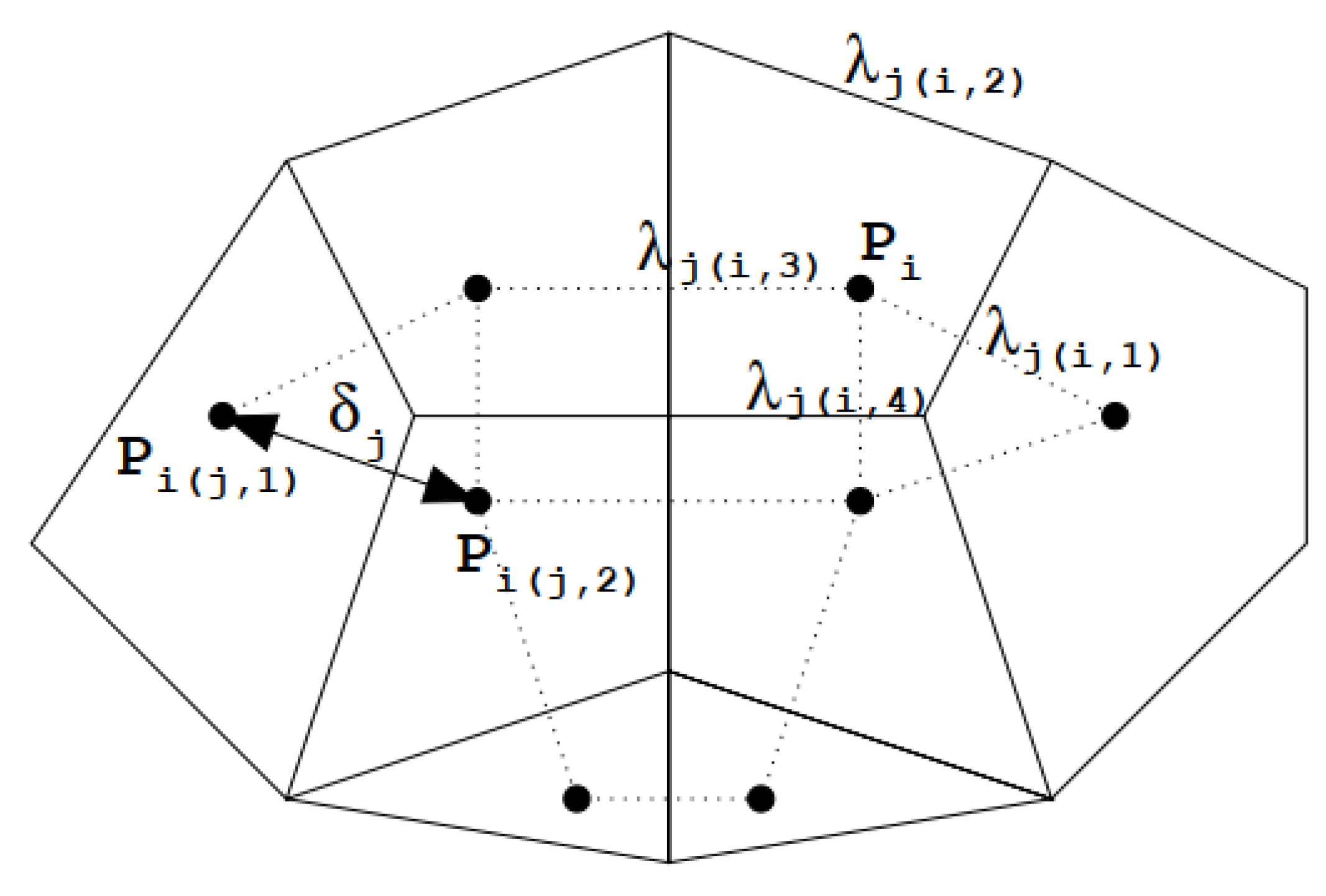
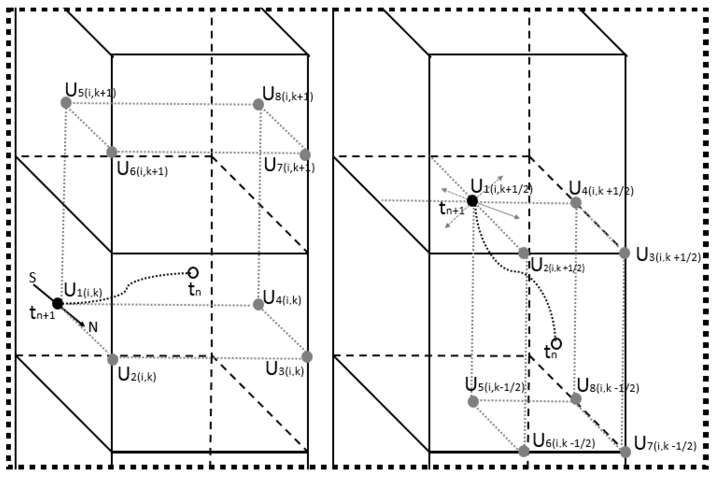
- For each time step, the particle starts at the barycenter of the j-th face at layer k, where the multistep backward Euler stream line is defined by linear interpolations to find the particle position at the end of a sub-time step (ELM step-i);
- (2)
- For each sub-time step, the particle position is analyzed in relation to the initial position (up-right, up-left, down-right, or down-left);
- (3)
- Eight node points are selected in the cell, with four points in layer k (the same layer where the particle stops) and four points in layer , depending on the particle position (up or down). The used points are always 4-face barycenters and 4 edge centers, except for the top and bottom cells, which uses 2-face barycenters, 4 edge centers, and 2 nodes;
- (4)
- The node indices are defined anticlockwise, where the first node is the initial position of the particle at time n+1;
- (5)
- Equation (31) is used to calculate the velocity component in the particle position in the sub-time step;
- (6)
- Steps (1–5) are repeated until the end of the Lagrangian trajectory.
- (1)
- For each time step, the particle starts at the horizontal-face barycenter of the i-th element at layer , where the multistep backward Euler stream line is defined by linear interpolations to find the particle position at the end of a sub-time step (ELM step-i)
- (2)
- For each sub-time step, the particle position is analyzed in relation to the initial position (up or down and in the direction of one of the four quadrants)
- (3)
- Eight node points are selected in the cell, with four points in layer (the same layer where the particle starts) and four points in layer , if the particle goes down, or , if the particle goes up. The used point always has a two-horizontal face barycenter, 4 edge centers, and 2 nodes;
- (4)
- The node indices are defined anticlockwise, where the first node is the initial position of the particle at time .
- (5)
- Equation (31) is used to calculate the velocity component in the particle position in the sub-time step.
- (6)
- Steps (1–5) are repeated until the end of the Lagrangian trajectory.
3.3. Quadratic Interpolator
- (1)
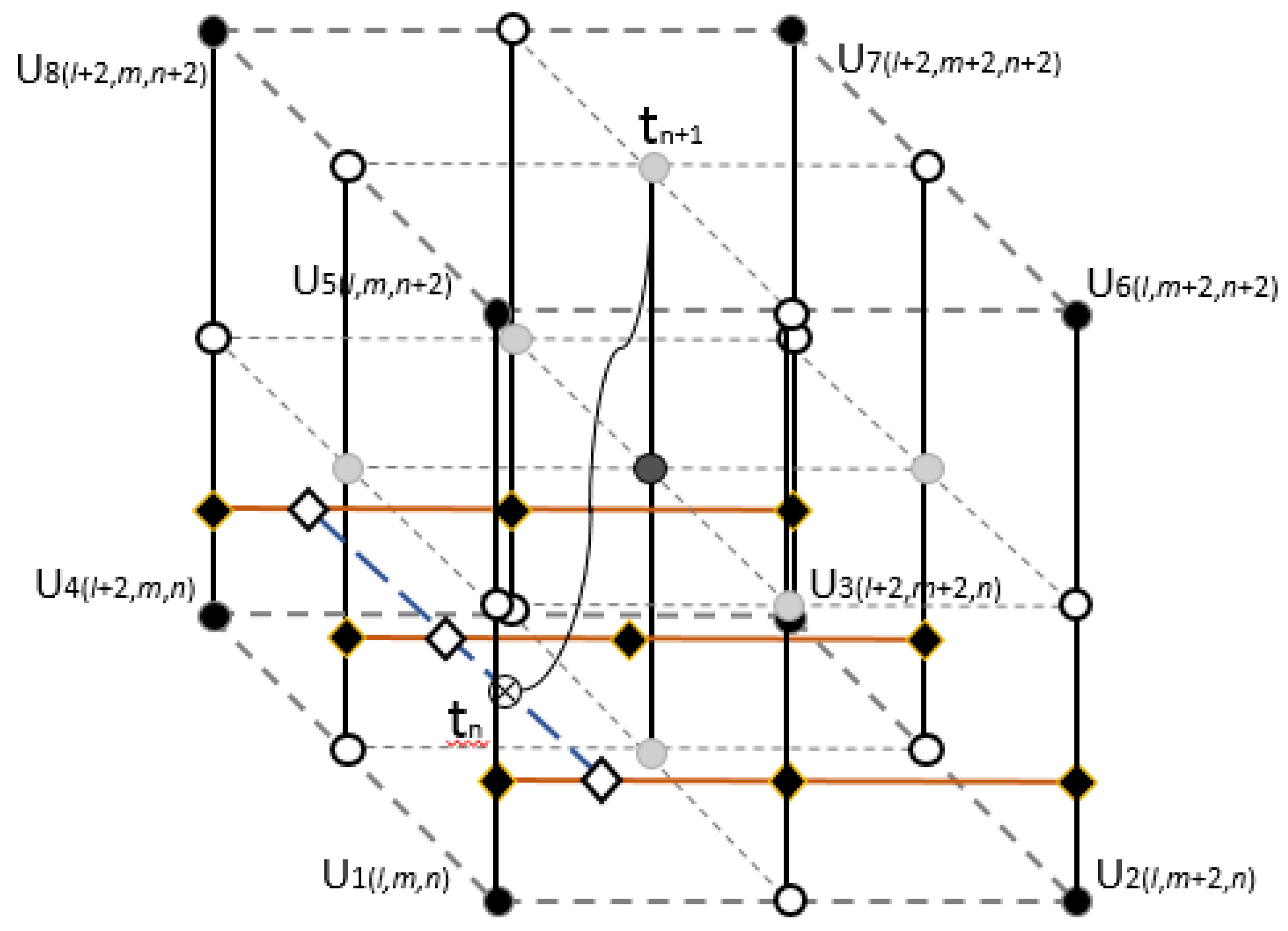
- First, 9 z-direction interpolations are carried out (black lines in Figure 3). Each vertical interpolation generates a velocity component in the horizontal plane that passes through the z-position of the particle, given bywhere each is multiplied by the respective velocity node and and are the “l” and “m” displacement, respectively, to indicate which vertical line has been interpolated.
- (2)
- Three x-direction interpolations are carried out (orange line), using the estimated velocities found in step (1), resulting in three new velocity components (white diamonds in Figure 3), given by
- (3)
- One interpolation is made to compute the y-direction displacement and find the final velocity for the particle at time
- (4)
- A new departure velocity is used to define the particle position in the next sub-time step.
- (5)
- Steps (1–4) are repeated until the end of the Lagrangian trajectory.
4. Numerical Experiments
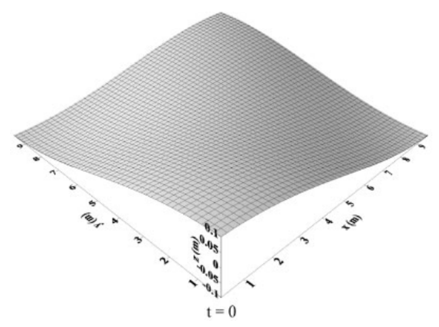
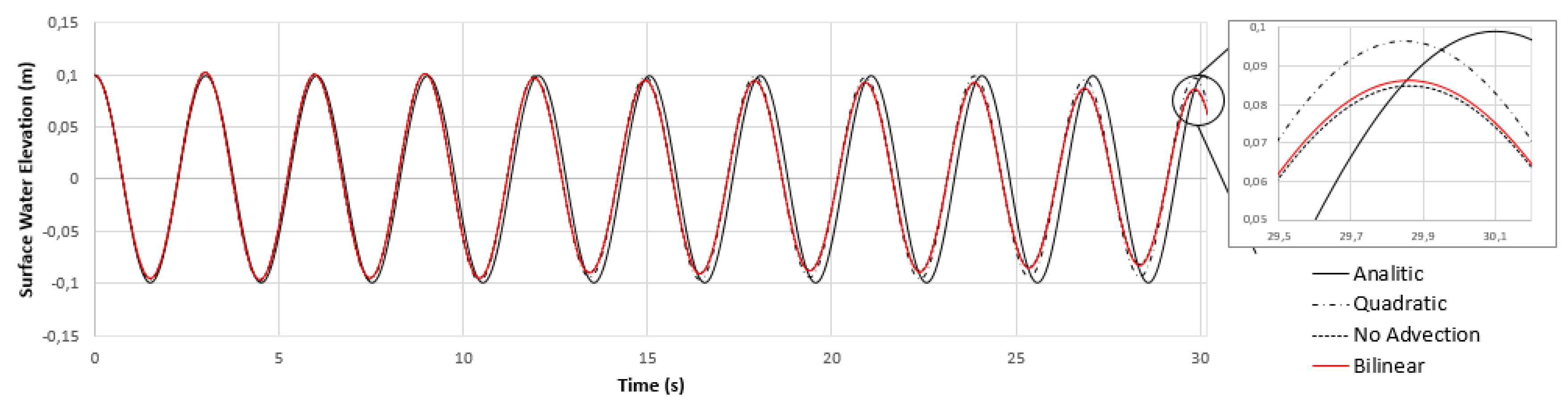
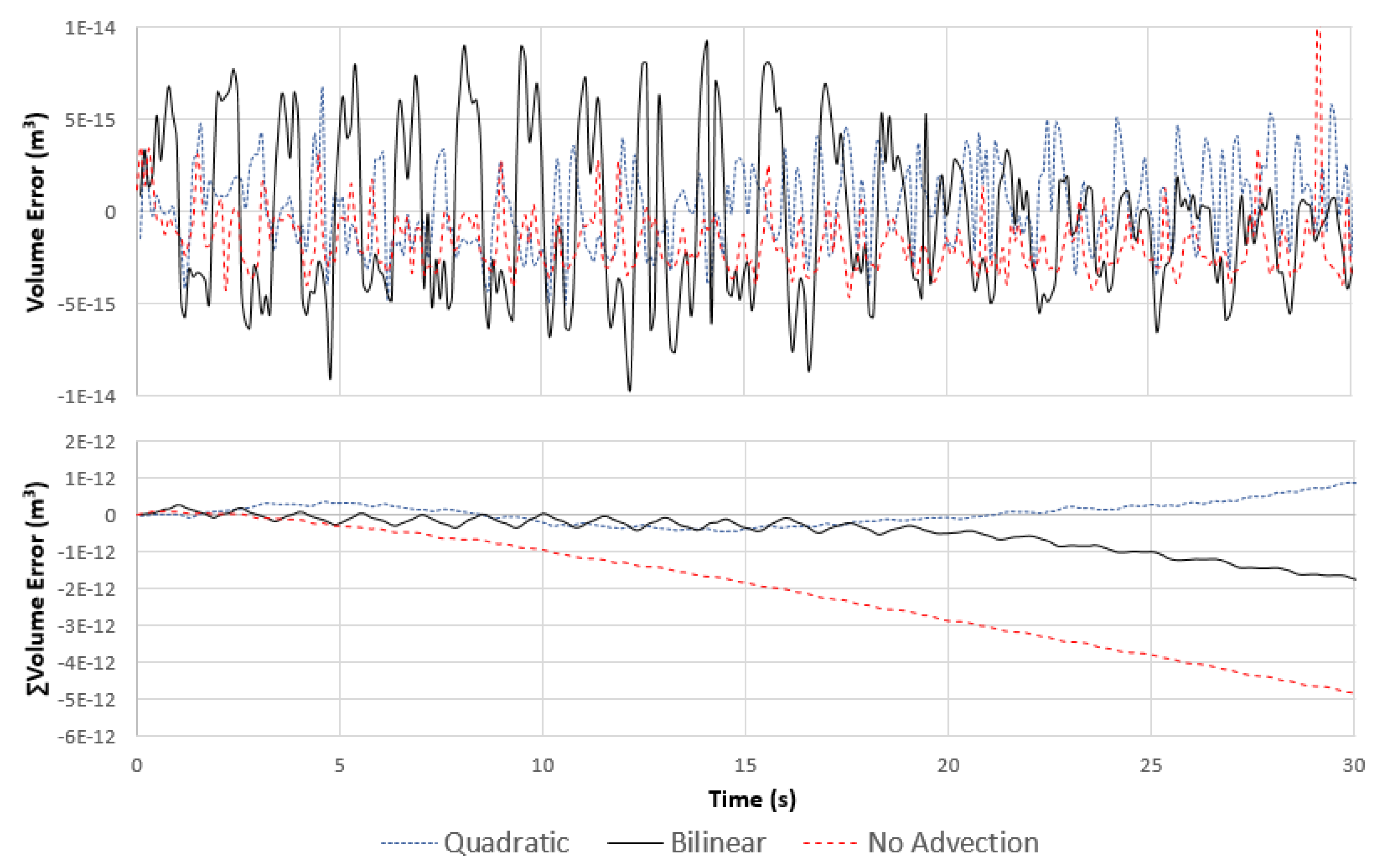
- Standing waves in a three-dimensional closed basin: this test case verifies the capability of the model to simulate 3D linear waves, including phase and amplitude representation [6,20,48]. The motion in the basin is caused only by the initial condition of the free surface. When the roughness, viscosity and diffusivity coefficients are set equal to zero, the motion of the free surface should not lose energy. However, a wave damping is caused by the numerical diffusion of the hydrodynamic solution. We evaluated the differences in the numerical diffusion between the bilinear and quadratic interpolations, applied in ELM step-ii, as well as the numerical diffusion considering the no-advection scheme.We also compared the mass conservation of the computation domain for each time step, the cumulative mass conservation over the course of the simulation, and the mean computation time of one time-step simulation.
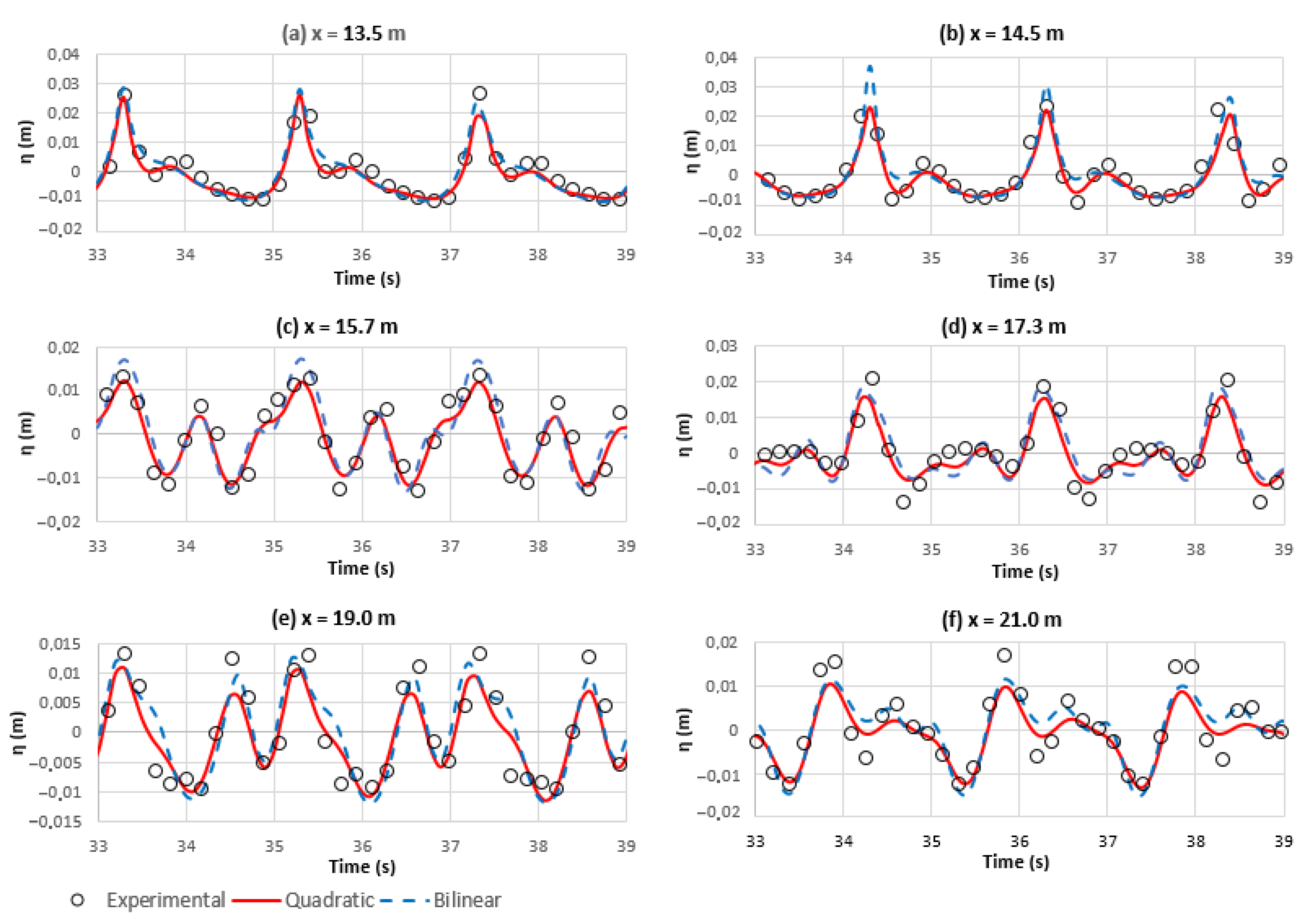
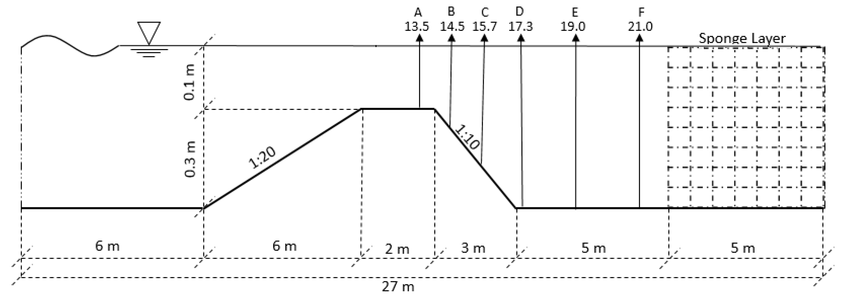
- Wave propagation over a submerged bar: this was an experimental model idealized by Beji and Battjes [50], and has been frequently used to validate numerical models (e.g., [4,47,48,49,51,52,53]). The experiment was used to evaluate the accuracy of representing an irregular wave pattern caused by physical changes at the bottom, by comparing the quadratic and bilinear interpolations used in ELM step-ii.
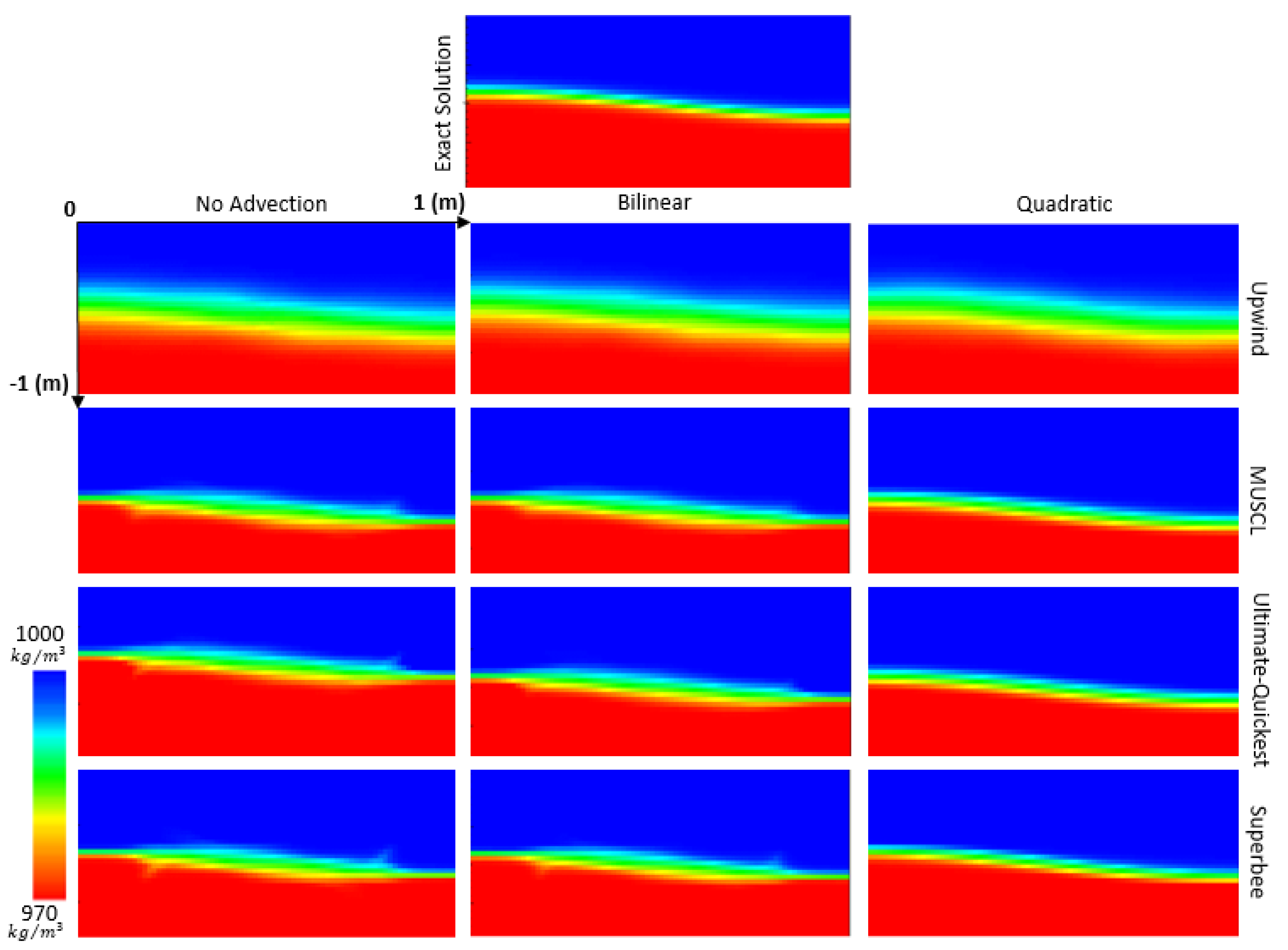
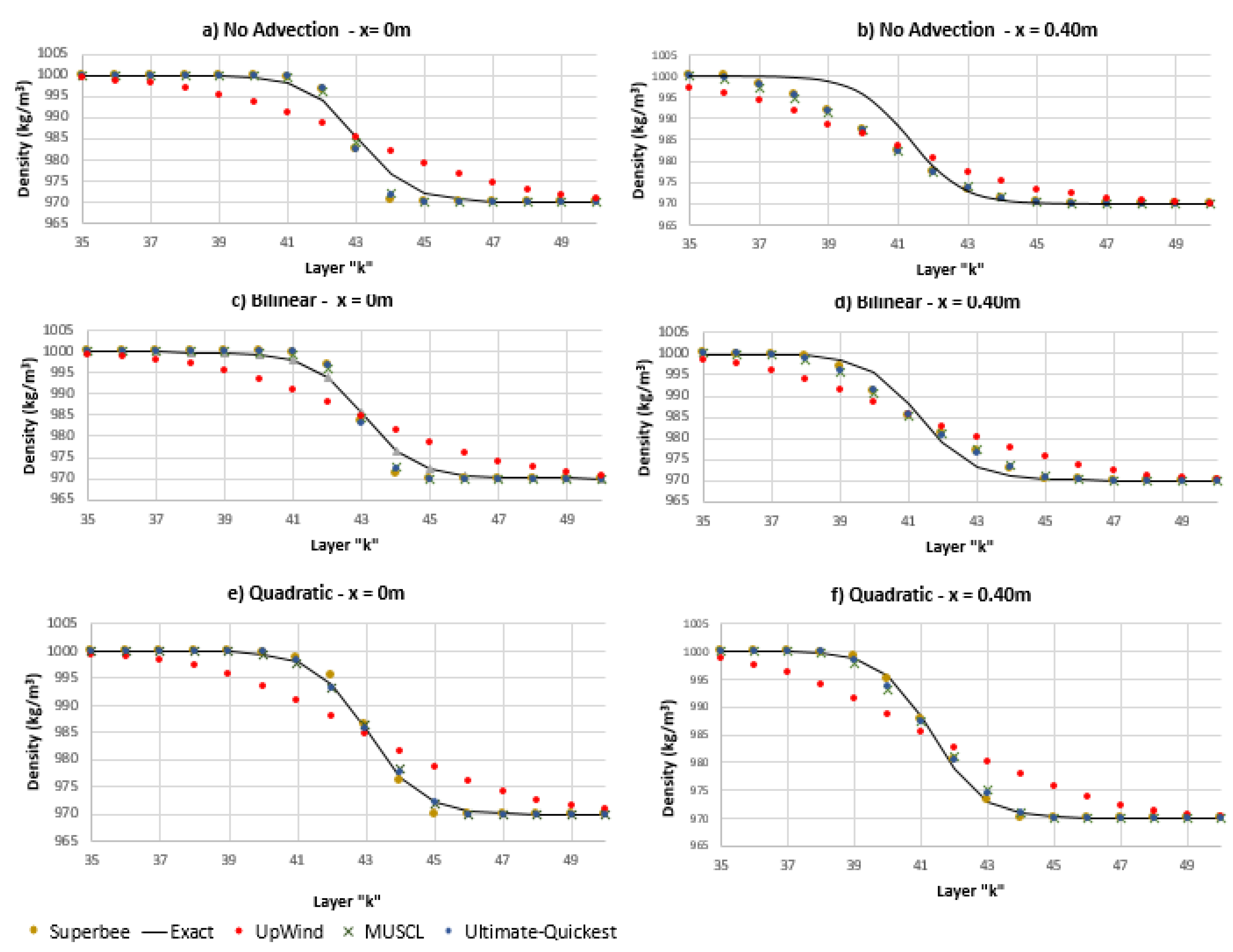
- Gravity wave test: consists of a finite-amplitude deep-water standing wave in an inviscid fluid in a nonequilibrium situation, where the baroclinic pressure makes a major contribution to promote flow. The experiment evaluated the numerical diffusion in terms of density interface expansion, analyzing the difference between the combined uses of the interpolation techniques used in ELM step-ii and different flux-limiter schemes applied in a solute transport solution. This test case also evaluated the individual effect of each interpolation technique used in the hydrodynamic solution on the solute transport solution, using different flux limiters. We also compared the mean computation time of one time-step simulation.
4.1. 3D Standing Waves in a Closed Basin
4.2. Wave Propagation over a Submerged Bar
4.3. Gravity Wave
5. Discussion
6. Conclusions
Author Contributions
Funding
Acknowledgments
Conflicts of Interest
References
- Marshall, J.; Hill, C.; Perelman, L.; Adcroft, A. Hydrostatic, quasi-hydrostatic, and nonhydrostatic ocean modeling. J. Geophys. Res. Oceans 1997, 102, 5733–5752. [Google Scholar] [CrossRef]
- Casulli, V.; Stelling, G.S. Numerical simulation of 3D quasi-hydrostatic, free-surface flows. J. Hydraul. Eng. 1998, 124, 678–686. [Google Scholar] [CrossRef]
- Chen, X. A fully hydrodynamic model for three-dimensional, free-surface flows. Int. J. Numer. Methods Fluids 2003, 42, 929–952. [Google Scholar] [CrossRef]
- Stelling, G.; Zijlema, M. An accurate and efficient finite-difference algorithm for nonhydrostatic free-surface flow with application to wave propagation. Int. J. Numer. Methods Fluids 2003, 43, 1–23. [Google Scholar] [CrossRef]
- Casulli, V.; Lang, G. Mathematical Model UnTRIM, Validation Document 1.0; The Federal Waterways Engineering and Research Institute (BAW): Hamburg, Germany, 2004. [Google Scholar]
- Liu, X.; Ma, D.G.; Zhang, Q.H. A higher-efficient nonhydrostatic finite volume model for strong three-dimensional free surface flows and sediment transport. China Ocean Eng. 2017, 31, 736–746. [Google Scholar] [CrossRef]
- Cheng, R.T.; Casulli, V.; Milford, S.N. Eulerian–Lagrangian solution of the convection-dispersion equation in natural coordinates. Water Resour. Res. 1984, 20, 944–952. [Google Scholar] [CrossRef]
- Ruan, F.; McLaughlin, D. An investigation of Eulerian–Lagrangian Methods for solving heterogeneous advection-dominated transport problems. Water Resour. Res. 1999, 35, 2359–2373. [Google Scholar] [CrossRef]
- Waterson, N.P.; Deconinck, H. Design principles for bounded higher-order convection schemes—A unified approach. J. Comput. Phys. 2007, 224, 182–207. [Google Scholar] [CrossRef]
- Kong, J.; Xin, P.; Shen, C.J.; Song, Z.Y.; Li, L. A high-resolution method for the depth-integrated solute transport equation based on an unstructured mesh. Environ. Model. Softw. 2013, 40, 109–127. [Google Scholar] [CrossRef]
- Ye, R.; Zhang, C.; Kong, J.; Jin, G.; Zhao, H.; Song, Z.; Li, L. A non-negative and high-resolution finite volume method for the depth-integrated solute transport equation using an unstructured triangular mesh. Environ. Fluid Mech. 2018, 18, 1379–1411. [Google Scholar] [CrossRef]
- Wang, H.; Lacroix, M. Interpolation techniques applied to the Eulerian–Lagrangian solution of the convection-dispersion equation in natural coordinates. Comput. Geosci. 1997, 23, 677–688. [Google Scholar] [CrossRef]
- Cox, T.; Runkel, R. Eulerian–Lagrangian numerical scheme for simulating advection, dispersion, and transient storage in streams and a comparison of numerical methods. J. Environ. Eng. 2008, 134, 996–1005. [Google Scholar] [CrossRef]
- Casulli, V.; Cheng, R.T. Semi-implicit finite difference methods for three-dimensional shallow water flow. Int. J. Numer. Methods Fluids 1992, 15, 629–648. [Google Scholar] [CrossRef]
- Jankowski, J.A. A Nonhydrostatic Model for Free Surface Flows. Ph.D. Thesis, Inst. für Strömungsmechanik und Elektronisches Rechnen im Bauwesen, Hannover, Germany, 1999. [Google Scholar]
- Hodges, B.R.; Imberger, J.; Saggio, A.; Winters, K.B. Modeling basin-scale internal waves in a stratified lake. Limnol. Oceanogr. 2000, 45, 1603–1620. [Google Scholar] [CrossRef] [Green Version]
- Wadzuk, B.M.; Hodges, B.R. Hydrostatic and Nonhydrostatic Internal Wave Models; Technical Report; Center for Research in Water Resources, University of Texas at Austin: Austin, TX, USA, 2004. [Google Scholar]
- Walters, R.A. A semi-implicit finite element model for nonhydrostatic (dispersive) surface waves. Int. J. Numer. Methods Fluids 2005, 49, 721–737. [Google Scholar] [CrossRef]
- Fringer, O.; Armfield, S.; Street, R. Reducing numerical diffusion in interfacial gravity wave simulations. Int. J. Numer. Methods Fluids 2005, 49, 301–329. [Google Scholar] [CrossRef]
- Monteiro, L.R.; Schettini, E.B.C. Comparação entre a aproximação hidrostática e a não-hidrostática na simulação numérica de escoamentos com superfície livre. Rev. Bras. De Recur. Hídricos 2015, 20, 1051–1062. [Google Scholar]
- Staniforth, A.; Côté, J. Semi-Lagrangian integration schemes for atmospheric models—A review. Mon. Weather Rev. 1991, 119, 2206–2223. [Google Scholar] [CrossRef]
- Oliveira, A.; Baptista, A.M. On the role of tracking on Eulerian–Lagrangian solutions of the transport equation. Adv. Water Resour. 1998, 21, 539–554. [Google Scholar] [CrossRef]
- Hodges, B.R.; Laval, B.; Wadzuk, B.M. Numerical error assessment and a temporal horizon for internal waves in a hydrostatic model. Ocean Model. 2006, 13, 44–64. [Google Scholar] [CrossRef]
- Laval, B.; Imberger, J.; Hodges, B.R.; Stocker, R. Modeling circulation in lakes: Spatial and temporal variations. Limnol. Oceanogr. 2003, 48, 983–994. [Google Scholar] [CrossRef] [Green Version]
- Laval, B.E.; Imberger, J.; Findikakis, A.N. Dynamics of a large tropical lake: Lake Maracaibo. Aquat. Sci. 2005, 67, 337–349. [Google Scholar] [CrossRef]
- Valipour, R.; Bouffard, D.; Boegman, L.; Rao, Y.R. Near-inertial waves in Lake Erie. Limnol. Oceanogr. 2015, 60, 1522–1535. [Google Scholar] [CrossRef]
- Vilas, M.P.; Marti, C.L.; Adams, M.P.; Oldham, C.E.; Hipsey, M.R. Invasive macrophytes control the spatial and temporal patterns of temperature and dissolved oxygen in a shallow lake: A proposed feedback mechanism of macrophyte loss. Front. Plant Sci. 2017, 8, 2097. [Google Scholar] [CrossRef]
- Soulignac, F.; Vinçon-Leite, B.; Lemaire, B.J.; Martins, J.R.S.; Bonhomme, C.; Dubois, P.; Mezemate, Y.; Tchiguirinskaia, I.; Schertzer, D.; Tassin, B. Performance Assessment of a 3D Hydrodynamic Model Using High Temporal Resolution Measurements in a Shallow Urban Lake. Environ. Model. Assess. 2017, 22, 309–322. [Google Scholar] [CrossRef]
- Boso, F.; Bellin, A.; Dumbser, M. Numerical simulations of solute transport in highly heterogeneous formations: A comparison of alternative numerical schemes. Adv. Water Resour. 2013, 52, 178–189. [Google Scholar] [CrossRef]
- Casulli, V.; Zanolli, P. High resolution methods for multidimensional advection–diffusion problems in free-surface hydrodynamics. Ocean Model. 2005, 10, 137–151. [Google Scholar] [CrossRef]
- Zhang, J.; Liang, D.; Liu, H. A hybrid hydrostatic and nonhydrostatic numerical model for shallow flow simulations. Estuar. Coast. Shelf Sci. 2018, 205, 21–29. [Google Scholar] [CrossRef]
- Sweby, P.K. High resolution schemes using flux limiters for hyperbolic conservation laws. SIAM J. Numer. Anal. 1984, 21, 995–1011. [Google Scholar] [CrossRef]
- Zhang, Z.; Song, Z.Y.; Kong, J.; Hu, D. A new r-ratio formulation for TVD schemes for vertex-centered FVM on an unstructured mesh. Int. J. Numer. Methods Fluids 2015, 81, 741–764. [Google Scholar] [CrossRef]
- Nangia, N.; Griffith, B.E.; Patankar, N.A.; Bhalla, A.P.S. A robust incompressible Navier–Stokes solver for high density ratio multiphase flows. arXiv 2019, arXiv:1809.01008. [Google Scholar] [CrossRef]
- Chandran, K.; Saha, A.K.; Mohapatra, P.K. Simulation of free surface flows with nonhydrostatic pressure distribution. Sādhanā 2019, 44, 20. [Google Scholar] [CrossRef]
- Jin, K.R.; Ji, Z.G. Application and validation of three-dimensional model in a shallow lake. J. Waterw. Port Coast. Ocean Eng. 2005, 131, 213–225. [Google Scholar] [CrossRef]
- Cavalcanti, J.R.; Motta-Marques, D.; Fragoso, C.R., Jr. Process-based modeling of shallow lake metabolism: Spatio-temporal variability and relative importance of individual processes. Ecol. Model. 2016, 323, 28–40. [Google Scholar] [CrossRef]
- Tang, X.; Chao, J.; Gong, Y.; Wang, Y.; Wilhelm, S.W.; Gao, G. Spatiotemporal dynamics of bacterial community composition in large shallow eutrophic Lake Taihu: High overlap between free-living and particle-attached assemblages. Limnol. Oceanogr. 2017, 62, 1366–1382. [Google Scholar] [CrossRef]
- Munar, A.M.; Cavalcanti, J.R.; Bravo, J.M.; Fan, F.M.; Motta-Marques, D.; Fragoso, C.R., Jr. Coupling large-scale hydrological and hydrodynamic modeling: Toward a better comprehension of watershed-shallow lake processes. J. Hydrol. 2018, 564, 424–441. [Google Scholar] [CrossRef]
- Casulli, V. Semi-implicit finite difference methods for the two-dimensional shallow water equations. J. Comput. Phys. 1990, 86, 56–74. [Google Scholar] [CrossRef]
- Cavalcanti, J.R.; Dumbser, M.; Motta-Marques, D.; Fragoso, C.R., Jr. A conservative finite volume scheme with time-accurate local time stepping for scalar transport on unstructured grids. Adv. Water Resour. 2015, 86, 217–230. [Google Scholar] [CrossRef]
- Van Leer, B. Towards the ultimate conservative difference scheme. V. A second-order sequel to Godunov’s method. J. Comput. Phys. 1979, 32, 101–136. [Google Scholar] [CrossRef]
- Roe, P.L. Characteristic-based schemes for the Euler equations. Annu. Rev. Fluid Mech. 1986, 18, 337–365. [Google Scholar] [CrossRef]
- Leonard, B. The ULTIMATE conservative difference scheme applied to unsteady one-dimensional advection. Comput. Methods Appl. Mech. Eng. 1991, 88, 17–74. [Google Scholar] [CrossRef]
- Darwish, M.; Moukalled, F. TVD schemes for unstructured grids. Int. J. Heat Mass Transf. 2003, 46, 599–611. [Google Scholar] [CrossRef]
- Li, Y.; Huang, P. A coupled lattice Boltzmann model for advection and anisotropic dispersion problem in shallow water. Adv. Water Resour. 2008, 31, 1719–1730. [Google Scholar] [CrossRef]
- Dingemans, M. Comparison of computations with Boussinesq-like models and laboratory measurements. In Memo in Framework of MAST Project (G8-M), Delft Hydraulics Memo H1684. 12; Deltares: Delft, The Netherlands, 1994. [Google Scholar]
- Yuan, H.; Wu, C.H. An implicit three-dimensional fully nonhydrostatic model for free-surface flows. Int. J. Numer. Methods Fluids 2004, 46, 709–733. [Google Scholar] [CrossRef]
- Yin, J.; Sun, J.W.; Wang, X.G.; Yu, Y.H.; Sun, Z.C. A hybrid finite-volume and finite difference scheme for depth-integrated nonhydrostatic model. China Ocean Eng. 2017, 31, 261–271. [Google Scholar] [CrossRef]
- Beji, S.; Battjes, J. Experimental investigation of wave propagation over a bar. Coast. Eng. 1993, 19, 151–162. [Google Scholar] [CrossRef]
- Beji, S.; Battjes, J. Numerical simulation of nonlinear wave propagation over a bar. Coast. Eng. 1994, 23, 1–16. [Google Scholar] [CrossRef]
- Zijlema, M.; Stelling, G.S. Further experiences with computing nonhydrostatic free-surface flows involving water waves. Int. J. Numer. Methods Fluids 2005, 48, 169–197. [Google Scholar] [CrossRef]
- Cui, H.; Pietrzak, J.; Stelling, G. Improved efficiency of a nonhydrostatic, unstructured grid, finite volume model. Ocean Model. 2012, 54, 55–67. [Google Scholar] [CrossRef]
- Park, J.C.; Kim, M.H.; Miyata, H. Fully nonlinear free-surface simulations by a 3D viscous numerical wave tank. Int. J. Numer. Methods Fluids 1999, 29, 685–703. [Google Scholar] [CrossRef]
- Thorpe, S. On standing internal gravity waves of finite amplitude. J. Fluid Mech. 1968, 32, 489–528. [Google Scholar] [CrossRef]
- Casulli, V. A semi-implicit finite difference method for nonhydrostatic, free-surface flows. Int. J. Numer. Methods Fluids 1999, 30, 425–440. [Google Scholar] [CrossRef]


| Metrics | Quadratic | Bilinear | No-Advection |
|---|---|---|---|
| RMSE (mm) | 21.86 | 20.80 | 20.70 |
| BIAS (mm) | 0.18 | 0.52 | 0.56 |
| Error (%) | 27.22 | 25.94 | 25.79 |
| KGE | 0.87 | 0.66 | 0.64 |
| NSE | 0.90 | 0.91 | 0.91 |
| M | Station a: x = 13.5 m | Station d: x = 17.3 m | ||
|---|---|---|---|---|
| Bilinear | Quadratic | Bilinear | Quadratic | |
| RMSE (mm) | 3.57 | 2.17 | 5.18 | 4.29 |
| BIAS (mm) | 2.01 | 0.18 | 0.87 | −0.56 |
| Error (%) | 47.52 | 23.65 | 83.78 | 60.00 |
| KGE | −0.90 | 0.82 | 0.23 | 0.46 |
| NSE | 0.83 | 0.94 | 0.56 | 0.70 |
| Station b:x= 14.5 m | Station e:x= 19.0 m | |||
| RMSE (mm) | 4.79 | 4.25 | 4.97 | 3.81 |
| BIAS (mm) | 0.14 | −0.64 | 2.49 | 0.76 |
| Error (%) | 64.77 | 50.22 | 52.79 | 45.31 |
| KGE | 0.39 | 0.35 | −6.12 | −1.18 |
| NSE | 0.33 | 0.47 | 0.60 | 0.76 |
| Station c:x= 15.7 m | Station f:x= 21.0 m | |||
| RMSE (mm) | 4.66 | 3.51 | 4.04 | 3.67 |
| BIAS (mm) | −0.19 | −1.25 | 1.34 | −0.28 |
| Error (%) | 56.71 | 39.63 | 57.48 | 43.84 |
| KGE | 0.65 | −1.07 | −4.92 | −0.26 |
| NSE | 0.67 | 0.81 | 0.69 | 0.75 |
| Flux Limiters | Fringer et al., 2005 | |||
|---|---|---|---|---|
| UpWind | 5.10 | 4.98 | 4.98 | 3.9 |
| MUSCL | 1.66 | 1.23 | 0.48 | 0.6 |
| Ultimate-Quickest | 1.40 | 0.94 | 0.46 | 0.4 |
| SuperBee | 1.36 | 0.88 | 0.30 | 0.4 |
| Flux Limiters | RMSE | RMSE | RMSE |
|---|---|---|---|
| Upwind | 2.08 | 1.97 | 1.97 |
| MUSCL | 1.16 | 0.72 | 0.38 |
| Ultimate-Quickest | 1.15 | 0.69 | 0.28 |
| Superbee | 1.16 | 0.70 | 0.24 |
© 2019 by the authors. Licensee MDPI, Basel, Switzerland. This article is an open access article distributed under the terms and conditions of the Creative Commons Attribution (CC BY) license (http://creativecommons.org/licenses/by/4.0/).
Share and Cite
Cunha, A.H.F.; Fragoso, C.R.; Tavares, M.H.; Cavalcanti, J.R.; Bonnet, M.-P.; Motta-Marques, D. Combined Use of High-Resolution Numerical Schemes to Reduce Numerical Diffusion in Coupled Nonhydrostatic Hydrodynamic and Solute Transport Model. Water 2019, 11, 2288. https://doi.org/10.3390/w11112288
Cunha AHF, Fragoso CR, Tavares MH, Cavalcanti JR, Bonnet M-P, Motta-Marques D. Combined Use of High-Resolution Numerical Schemes to Reduce Numerical Diffusion in Coupled Nonhydrostatic Hydrodynamic and Solute Transport Model. Water. 2019; 11(11):2288. https://doi.org/10.3390/w11112288
Chicago/Turabian StyleCunha, Augusto Hugo Farias, Carlos Ruberto Fragoso, Matheus Henrique Tavares, J. Rafael Cavalcanti, Marie-Paule Bonnet, and David Motta-Marques. 2019. "Combined Use of High-Resolution Numerical Schemes to Reduce Numerical Diffusion in Coupled Nonhydrostatic Hydrodynamic and Solute Transport Model" Water 11, no. 11: 2288. https://doi.org/10.3390/w11112288
APA StyleCunha, A. H. F., Fragoso, C. R., Tavares, M. H., Cavalcanti, J. R., Bonnet, M.-P., & Motta-Marques, D. (2019). Combined Use of High-Resolution Numerical Schemes to Reduce Numerical Diffusion in Coupled Nonhydrostatic Hydrodynamic and Solute Transport Model. Water, 11(11), 2288. https://doi.org/10.3390/w11112288