Spatial and Temporal Variations in Water Quality and Land Use in a Semi-Arid Catchment in Bolivia

 ,
,  ,
,
Abstract
1. Introduction
2. Materials and Methods
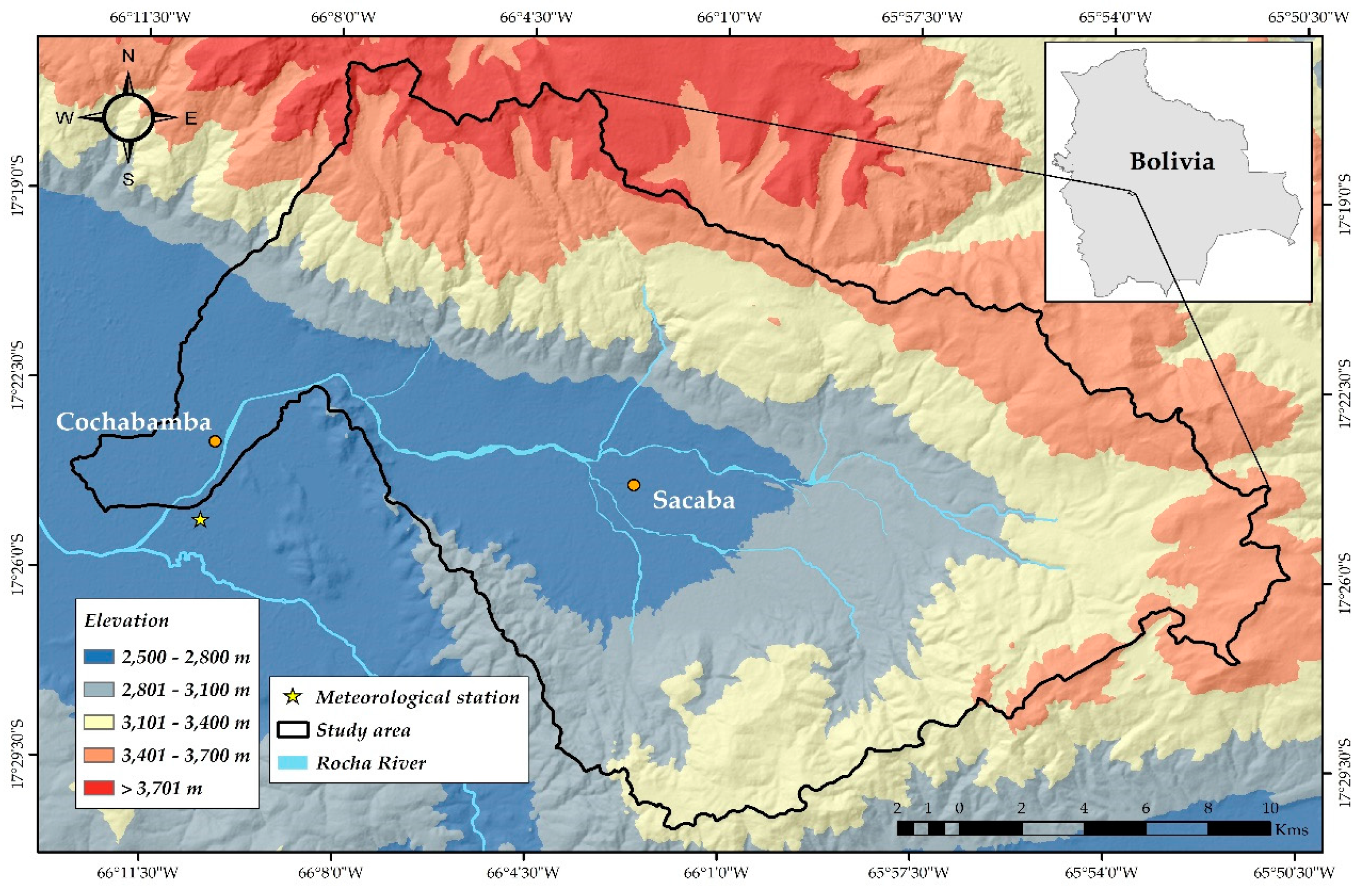
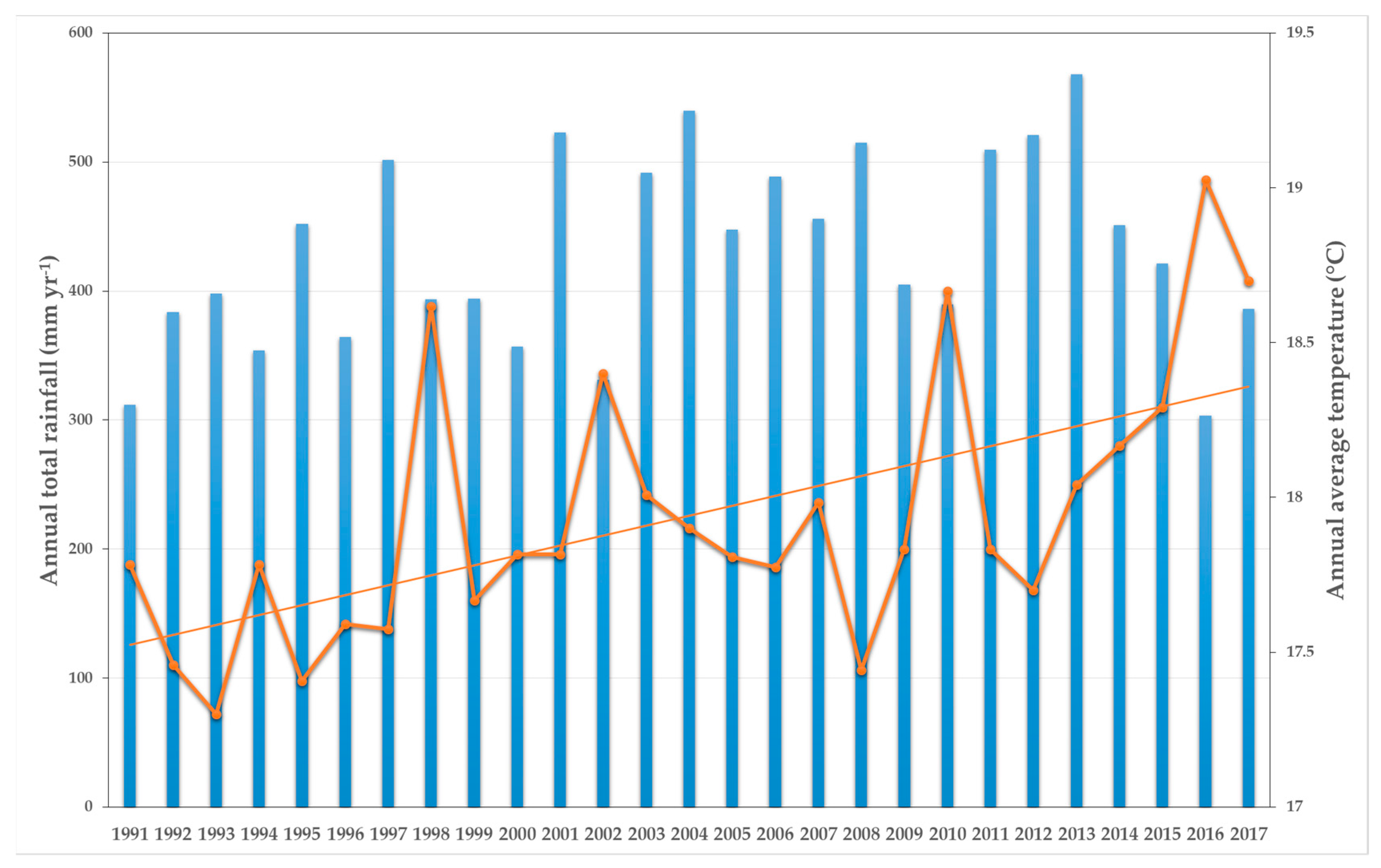
2.1. Study Area
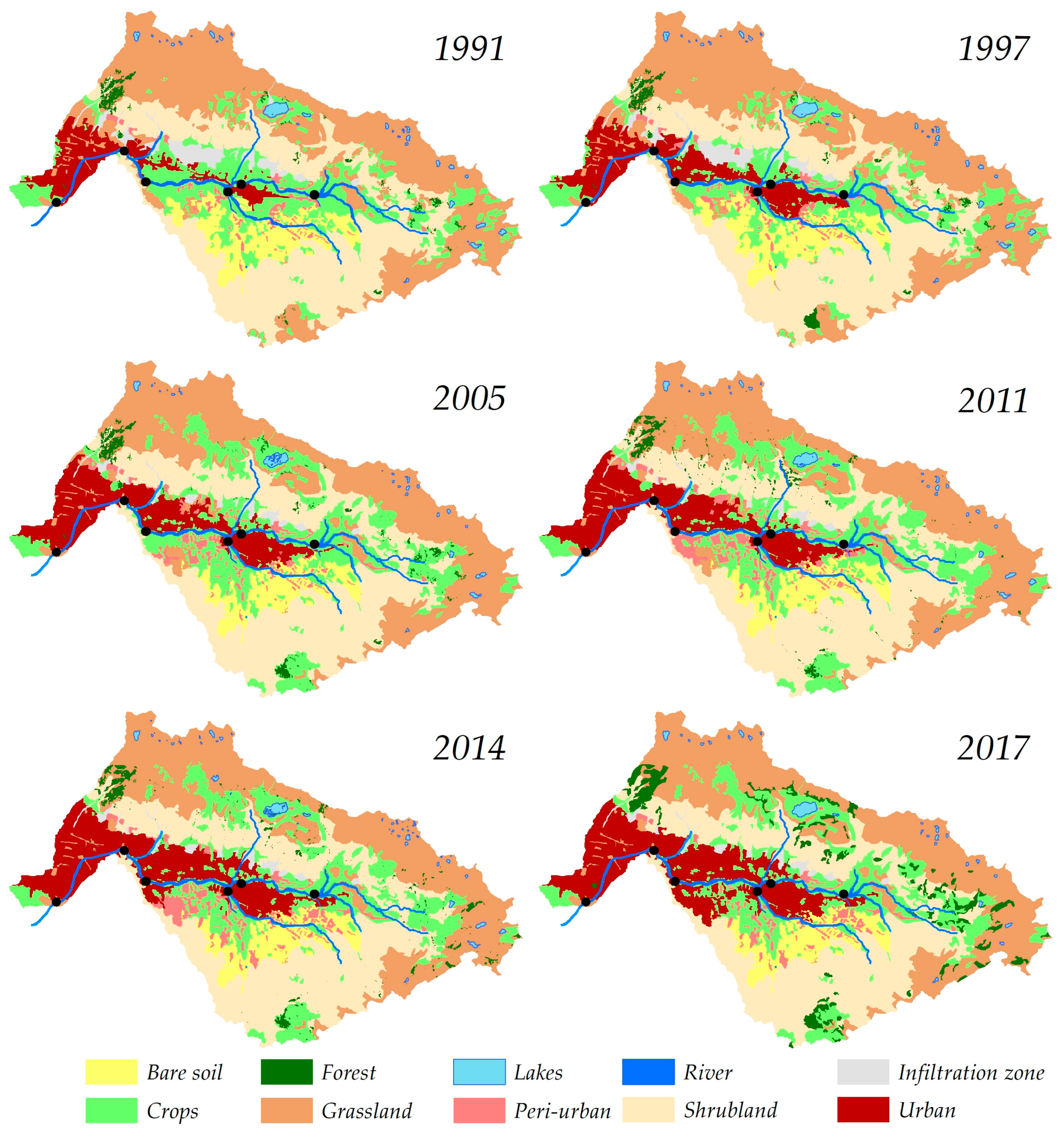
2.2. Land Use and Land Use Changes
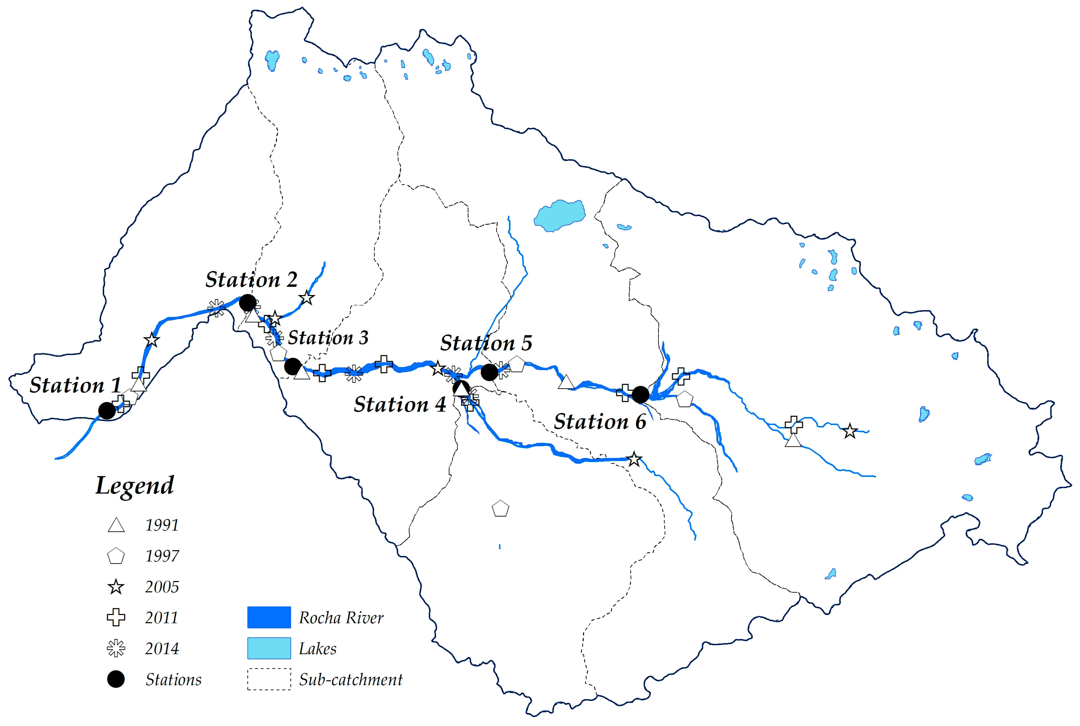
2.3. Data Collection and Sampling
2.4. Water Quality Indices
2.5. Relationship and Trend Analysis
3. Results
3.1. Land Use Analysis
3.2. Water Quality and Water Flow
3.3. Water Quality and Land Uses
4. Discussion
5. Conclusions
Supplementary Materials
Author Contributions
Funding
Acknowledgments
Conflicts of Interest
References
- Sajikumar, N.; Remya, R. Impact of land cover and land use change on runoff characteristics. J. Environ. Manag. 2015, 161, 460–468. [Google Scholar] [CrossRef] [PubMed]
- Miller, J.; Kim, H.; Kjeldsen, T.; Packman, J.; Grebby, S.; Dearden, R. Assessing the impact of urbanization on storm runoff in a peri-urban catchment using historical change in impervious cover. J. Hydrol. 2014, 515, 59–70. [Google Scholar] [CrossRef]
- Nie, W.; Yuan, Y.; Kepner, W.; Nash, M.; Jackson, M.; Erickson, C. Assessing impacts of landuse and landcover changes on hydrology for the upper San Pedro watershed. J. Hydrol. 2011, 407, 105–114. [Google Scholar] [CrossRef]
- Giri, S.; Qiu, Z. Understanding the relationship of land uses and water quality in Twenty First Century: A review. J. Environ. Manag. 2016, 173, 41–48. [Google Scholar] [CrossRef]
- Foley, J.; DeFries, R.; Asner, G.; Barford, C.; Bonan, G.; Carpenter, S.; Chapin, F.; Coe, M.; Daily, G.; Gibbs, H.; et al. Global consequences of land use. Science 2005, 309, 570–574. [Google Scholar] [CrossRef]
- Chu, H.; Liu, C.; Wang, C. Identifying the relationships between water quality and land cover changes in the Tseng-Wen reservoir watershed of Taiwan. Int. J. Environ. Res. Public Health 2013, 10, 478–489. [Google Scholar] [CrossRef]
- Kamarinas, I.; Julian, J.; Hughes, A.; Owsley, B.; De Beurs, K. Nonlinear changes in land cover and sediment runoff in a New Zealand catchment dominated by plantation forestry and livestock grazing. Water 2016, 8, 436. [Google Scholar] [CrossRef]
- Li, S.; Gu, S.; Liu, W.; Han, H.; Zhang, Q. Water quality in relation to land use and land cover in the upper Han River Basin, China. Catena 2008, 75, 216–222. [Google Scholar] [CrossRef]
- Haidary, A.; Amiri, B.; Adamowski, J.; Fohrer, N.; Nakane, K. Assessing the impacts of four land use types on the water quality of wetlands in Japan. Water Resour. Manag. 2013, 27, 2217–2229. [Google Scholar] [CrossRef]
- Tong, S.; Chen, W. Modeling the relationship between land use and surface water quality. J. Environ. Manag. 2002, 66, 377–393. [Google Scholar] [CrossRef]
- Ahearn, D.; Sheibley, R.; Dahlgren, R.; Anderson, M.; Johnson, J.; Tate, K. Land use and land cover influence on water quality in the last free-flowing river draining the western Sierra Nevada, California. J. Hydrol. 2005, 313, 234–247. [Google Scholar] [CrossRef]
- Tu, J. Spatially varying relationships between land use and water quality across an urbanization gradient explored by geographically weighted regression. Appl. Geogr. 2011, 31, 376–392. [Google Scholar] [CrossRef]
- Chen, Q.; Mei, K.; Dahlgren, R.; Wang, T.; Gong, J.; Zhang, M. Impacts of land use and population density on seasonal surface water quality using a modified geographically weighted regression. Sci. Total Environ. 2016, 572, 450–466. [Google Scholar] [CrossRef] [PubMed]
- Contraloria General del Estado. Informe de Auditoría Sobre el Desempeño Ambiental Respecto de los Impactos Negativos Generados en el Río Rocha; K2/AP06/M11; Gestión de Evaluación Ambiental: Cochabamba, Bolivia, 2011; p. 320.
- Gobierno Autónomo Municipal de Sacaba. Propuesta de Clasificación del río Rocha en Función a su Aptitud de Uso; Dirección de Madre Tierra y Medio Ambiente: Cochabamba, Bolivia, 2014; p. 167.
- Prefecture of the Departament of Cochabamba. Estudios Básicos de la Cuenca del Río Rocha; Prefecture of the Departament of Cochabamba: Cochabamba, Bolivia, 2005; p. 314.
- Romero, A.; Van Damme, P.; Goitia, E. Contaminación orgánica en el río Rocha (Cochabamba, Bolivia). Revista Boliviana de Ecología y Conservación Ambiental 1998, 8, 37–47. [Google Scholar]
- Coronado, O.; Moscoso, Ó.; Claros, L. Estudio de Viabilidad Cochabamba, Bolivia; Organización Panamericana de la Salud: Lima, Perú, 2002; p. 80. [Google Scholar]
- Dost, R. Hydrologic Information Systems as a Support Tool for Water Quality Monitoring A Case Study in the Bolivian Andes; Research, International Institute for Geo-information Science and Earth Observation: Enschede, The Netherlands, 2005. [Google Scholar]
- Gobierno Autónomo Municipal de Sacaba. Prácticas de Saneamiento Ambiental Sostenibles en la Cuenca del Río Maylanco; Consultora INAXO: Cochabmaba, Bolivia, 2011; p. 37.
- Bolivian Ministry of Environment and Water. Plan Maestro Metropolitano de Agua y Saneamiento del Área Metropolitana de Cochabamba Bolivia; Bolivian Ministry of Environment and Water: La paz, Bolivia, 2012; p. 680.
- Programa de Aguas; Programa de Hidronomia. Informe Tecnico IX, Monitoreo del Río Rocha; Universidad Mayor de San Simón: Cochabmba, Bolivia, 1992; p. 6. [Google Scholar]
- Toledo, R.; Amurrio, D. Evaluación de la calidad de las aguas del río Rocha en la jurisdicción de SEMAPA en la provincia Cercado de Cochabamba-Bolivia. Acta Nova 2006, 3, 521–542. [Google Scholar]
- Vergara, S. Indices de Calidad de agua Como Indicador De Contaminación Y Su Distribución Espacio-Temporal En El río Rocha. Magister profesional; Universidad Mayor de San Simón: Cochabamba, Bolivia, 2001. [Google Scholar]
- De La Mora-Orozco, C.; Flores-Lopez, H.; Rubio-Arias, H.; Chavez-Duran, A.; Ochoa-Rivero, J. Developing a Water Quality Index (WQI) for an irrigation dam. Int. J. Environ. Res. Public Health 2017, 14, 439. [Google Scholar] [CrossRef]
- Sutadian, A.; Muttil, N.; Yilmaz, A.; Perera, B. Development of river water quality indices—A review. Environ. Monit. Assess. 2016, 188, 58. [Google Scholar] [CrossRef]
- Horton, R. An index number system for rating water quality. J. Water Pollut. Control Fed. 1965, 37, 300–306. [Google Scholar]
- Brown, R.; McClelland, N.; Deininger, R.; Tozer, R. A Water Quality Index—Do we dare? Water Sew. Works 1970, 117, 339–343. [Google Scholar]
- Brown, R.; McClelland, N.; Deininger, R.; Landwehr, J. Validating the WQI. In Proceedings of the Paper Presented at National Meeting of American Society of Civil Engineers on Water Resources Engineering, Washington, DC, USA, 29 January–2 February 1973. [Google Scholar]
- Prati, L.; Pavanello, R.; Pesarin, F. Assessment of surface water quality by a single index of pollution. Water Res. 1971, 5, 741–751. [Google Scholar] [CrossRef]
- Lumb, A.; Sharma, T.; Bibeault, J. A Review of genesis and evolution of Water Quality Index (WQI) and some future directions. Water Qual. Expo. Health 2011, 3, 11–24. [Google Scholar] [CrossRef]
- Sener, S.; Sener, E.; Davraz, A. Evaluation of water quality using water quality index (WQI) method and GIS in Aksu River (SW-Turkey). Sci. Total Environ. 2017, 584–585, 131–144. [Google Scholar] [CrossRef] [PubMed]
- Ewaid, S.; Abed, S. Water quality index for Al-Gharraf River, southern Iraq. Egypt. J. Aquat. Res. 2017, 43, 117–122. [Google Scholar] [CrossRef]
- Kannel, P.R.; Lee, S.; Lee, Y.S.; Kanel, S.R.; Khan, S.P. Application of water quality indices and dissolved oxygen as indicators for river water classification and urban impact assessment. Environ. Monit. Assess. 2007, 132, 93–110. [Google Scholar] [CrossRef]
- Debels, P.; Figueroa, R.; Urrutia, R.; Barra, R.; Niell, X. Evaluation of water quality in the Chillan River (Central Chile) using physicochemical parameters and a modified water quality index. Environ. Monit. Assess. 2005, 110, 301–322. [Google Scholar] [CrossRef]
- Salcedo-Sánchez, E.; Hoyos, S.; Alberich, M.; Morales, M. Application of water quality index to evaluate groundwater quality (temporal and spatial variation) of an intensively exploited aquifer (Puebla valley, Mexico). Environ. Monit. Assess. 2016, 188, 573. [Google Scholar] [CrossRef]
- Instituto Nacional de Estadística. Principales Resultados del Censo Nacional de Población y Vivienda 2012; Estado Plutrinacional de Bolivia: La Paz, Bolivia, 2013; p. 56.
- Gobierno Autónomo Municipal de Sacaba. Plan Territorial de Desarrollo Integral—PTDT; Territorial, O., Ed.; Secretaria Municipal de Planificación y Desarrollo Territorial: Sacaba, Cochabamba, Bolivia, 2016; p. 294.
- Kennan, L.; Lamb, S.; Rundle, C. K-Ar Dates from the Altiplano and Cordillera-Oriental of Bolivia—Implications for cenozoic stratigraphy and tectonics. J. S. Am. Earth Sci. 1995, 8, 163–186. [Google Scholar] [CrossRef]
- Ongaro, L.; l’Oltremare, I.A.P.; Esteri, I.M.D.A. Land Evaluation of the Valley of Sacaba (Bolivia); Istituto agronomico per l’Oltremare: Firenze, Italy, 1998.
- Metternicht, G.; Fermont, A. Estimating erosion surface features by linear mixture modeling. Remote Sens. Environ. 1998, 64, 254–265. [Google Scholar] [CrossRef]
- Metternicht, G.; Gonzalez, S. FUERO: Foundations of a fuzzy exploratory model for soil erosion hazard prediction. Environ. Model. Softw. 2005, 20, 715–728. [Google Scholar] [CrossRef]
- Environmental Resources Management. Estudios Básicos de Mitigación y Adaptación al Cambio Climático, Vulnerabilidades, Huella Urbana Y Escenarios de Crecimiento Urbano Y Para La Región Metropolitana de Cochabamba; Inter-American Development Bank: Washington, DC, USA, 2013; p. 120. [Google Scholar]
- Congalton, R.; Green, K. Assessing the Accuracy of Remotely Sensed Data: Principles and Practices; CRC Press, Taylor and Francis Group: Boca Raton, FL, USA, 2008. [Google Scholar]
- Cohen, J. A Coefficient of agreement for nominal scales. Educ. Psychol. Meas. 1960, 20, 37–46. [Google Scholar] [CrossRef]
- Dirección de Madre Tierra y Medio Ambiente. Informe de Monitoreo Cuenca del Río Rocha—Sacaba; Gobierno Autónomo Municipal de Sacaba: Cochabamba, Bolivia, 2015; p. 24.
- Chilundo, M.; Kelderman, P.; Okeeffe, J. Design of a water quality monitoring network for the Limpopo River Basin in Mozambique. Phys. Chem. Earth 2008, 33, 655–665. [Google Scholar] [CrossRef]
- APHA; AWWA; WEF. Standard methods for the examination of water and wastewater. In Public Health Association; APHA: Washington, DC, USA, 1992; Volume 18. [Google Scholar]
- ASTM. Standards for Water and Wastewater; American Society for Testing Materials: Philadelphia, PA, USA, 1958. [Google Scholar]
- Abbasi, T.; Abbasi, S. ‘Conventional’ indices for determining fitness of waters for different uses. In Water Quality Indices; Elsevier: Amsterdam, The Netherlands, 2012; pp. 25–62. [Google Scholar] [CrossRef]
- Ott, W. Environmental Indices: Theory and Practice; Ann Arbor Science Publishers, Inc.: Ann Arbor, Michigan, USA, 1978; pp. 202–215. [Google Scholar]
- Hirsch, R.; Slack, J.; Smith, R. Techniques of trend analysis for monthly water quality data. Water Resour. Res. 1982, 18, 107–121. [Google Scholar] [CrossRef]
- Sheikhy, T.; Aris, A.; Sefie, A.; Keesstra, S. Detecting and predicting the impact of land use changes on groundwater quality, a case study in Northern Kelantan, Malaysia. Sci. Total Environ. 2017, 599–600, 844–853. [Google Scholar] [CrossRef] [PubMed]
- Du, X.; Huang, Z. Ecological and environmental effects of land use change in rapid urbanization: The case of hangzhou, China. Ecol. Indic. 2017, 81, 243–251. [Google Scholar] [CrossRef]
- Peredo, M.; Perez, J. Auditoria Especializada sobre el Desempeño Ambiental De Empresas Que Suministran Agua Potable A Las Ciudades de La Paz, El Alto y Cochabamba; Bachellor Project; University of San Andres: La Paz, Bolivia, 2010. [Google Scholar]
- Ayala, R.; Acosta, F.; Mooij, W.; Rejas, D.; Van Damme, P. Management of Laguna Alalay: A case study of lake restoration in Andean valleys in Bolivia. Aquat. Ecol. 2007, 41, 621–630. [Google Scholar] [CrossRef]
- Fries, A.; Rollenbeck, R.; Nauß, T.; Peters, T.; Bendix, J. Near surface air humidity in a megadiverse Andean mountain ecosystem of southern Ecuador and its regionalization. Agric. For. Meteorol. 2012, 152, 17–30. [Google Scholar] [CrossRef]
- Robledo, C.; Fischler, M.; Patiño, A. The Role of Community-Based Forest Land Rehabilitation in Building Resilience to Climate Impacts: A Case Study from the PROFOR-Afforestation Project in the Community of Khuluyo Cochabamba, Bolivia; Intercooperation Working Paper; Intercooperation: Bern, Switzerland, 2003. [Google Scholar]
- Wiese, K.; Klette, C. Save Bolivian Jungle. Available online: https://www.naturefund.de/en/about_us/our_vision/ (accessed on 20 July 2018).
- USER, S. Reforestation in Cochabamba, Bolivia. Available online: http://fontana-foundation.org/data3/index.php/en/closed-projects/reforestation-bolivia (accessed on 15 July 2018).
- Hasan, H.; Jamil, N.; Aini, N. Water quality index and sediment loading analysis in Pelus River, Perak, Malaysia. Procedia Environ. Sci. 2015, 30, 133–138. [Google Scholar] [CrossRef]
- Lai, Y.; Tu, Y.; Yang, C.; Surampalli, R.; Kao, C. Development of a water quality modeling system for river pollution index and suspended solid loading evaluation. J. Hydrol. 2013, 478, 89–101. [Google Scholar] [CrossRef]
- Ramos, M.; de Oliveira, E.; Piao, A.; Leite, D.; de Angelis, F. Water Quality Index (WQI) of Jaguari and Atibaia Rivers in the region of Paulinia, Sao Paulo, Brazil. Environ. Monit. Assess. 2016, 188, 263. [Google Scholar] [CrossRef][Green Version]
- Rubio-Arias, H.; Contreras-Caraveo, M.; Quintana, R.; Saucedo-Teran, R.A.; Pinales-Munguia, A. An overall Water Quality Index (WQI) for a man-made aquatic reservoir in Mexico. Int. J. Environ. Res. Public Health 2012, 9, 1687–1698. [Google Scholar] [CrossRef]
- Wang, Q.; Wu, X.; Zhao, B.; Qin, J.; Peng, T. Combined multivariate statistical techniques, Water Pollution Index (WPI) and Daniel Trend Test methods to evaluate temporal and spatial variations and trends of water quality at Shanchong River in the Northwest Basin of Lake Fuxian, China. PLoS ONE 2015, 10, e0118590. [Google Scholar] [CrossRef] [PubMed]
- de Souza, M.; Cavalheri, P.; de Oliveira, M.; Magalhães, F. A multivariate statistical approach to the integration of different land-uses, seasons, and water quality as water resources management tool. Environ. Monit. Assess. 2019, 191, 539. [Google Scholar] [CrossRef] [PubMed]
- Bora, M.; Goswami, D. Water quality assessment in terms of water quality index (WQI): Case study of the Kolong River, Assam, India. Appl. Water Sci. 2016, 7, 3125–3135. [Google Scholar] [CrossRef]
- Shi, B.; Bach, P.; Lintern, A.; Zhang, K.; Coleman, R.A.; Metzeling, L.; McCarthy, D.T.; Deletic, A. Understanding spatiotemporal variability of in-stream water quality in urban environments—A case study of Melbourne, Australia. J. Environ. Manag. 2019, 246, 203–213. [Google Scholar] [CrossRef] [PubMed]
- Carstens, D.; Amer, R. Spatio-temporal analysis of urban changes and surface water quality. J. Hydrol. 2019, 569, 720–734. [Google Scholar] [CrossRef]


| Parameter | Technique | Standard Method | Detection Limit |
|---|---|---|---|
| Dissolved oxygen | Membrane electrode Luminescence-based | SM4500-O C ASTM D888-05 | 0.05 mgO2/L 1 mgO2/L |
| Faecal coliforms | Membrane filter | SM 9222-D SM 9222-B | 0 UFC/mL |
| pH | Electrometric | ASTM D 1293-99 4500-HB | 0.01 pH 0.1 pH |
| Biological oxygen demand | Winkler dilution Dilution | SM 5210 B DIN 38409 | 2 mgO2/L 5 mgO2/L |
| Chemical oxygen demand | Dichromate oxidation | SM 5220 B ASTM D 1252-00 | 2 mgO2/L |
| Phosphates | Colorimetric | SM 2500-PO3 EPA 365.2 | 0.08 mgP/L 0.01 mgP/L |
| Nitrates | Cadmium reduction Colorimetric | SM 4500-NO3 DIN 38405 | 0.01 mgN–NO3/L |
| Turbidity | Nephelometric | 2130 B | 0.1 NTU |
| Total solids | Gravimetric—105 ˚C Colorimetric | SM 2540 B DIN 38409 H1 | 0.01 mg/L 1 mg/L |
| Parameter | Weight |
|---|---|
| Dissolved oxygen | 0.17 |
| Faecal coliforms | 0.16 |
| pH Biochemical oxygen demand | 0.11 0.11 |
| Phosphates Nitrates | 0.10 0.10 |
| Delta temperature | 0.10 |
| Turbidity | 0.08 |
| Total solids | 0.07 |
| Parameter | Units of Pollution | Value |
|---|---|---|
| Dissolved oxygen (DO) | 0–50% 50–100% >100% | |
| Biological oxygen demand (BOD) Chemical oxygen demand (COD) Nitrates (NO3) | mg/L mg/L mg/L | X3 = 0.1Y |
| Category | NSF-WQI Value | IPI Value | Colour Code |
|---|---|---|---|
| Not polluted | 91–100 | 0–1 | Blue |
| Acceptable | 71–90 | 1–2 | Green |
| Slightly polluted | 51–70 | 2–4 | Yellow |
| Polluted | 26–50 | 4–8 | Orange |
| Very polluted | – | 8–16 | Red |
| Heavily polluted | 0–25 | >16 | Black |
| Land Use | 1991 | 1991–1997 | 1997–2005 | 2005–2011 | 2011–2014 | 2014–2017 | 1991–2017 | 2017 | ||
|---|---|---|---|---|---|---|---|---|---|---|
| km2 | % | % | % | % | % | % | % | km2 | % | |
| Bare soil | 32.6 | 7 | 0 | −3 | −8 | 3 | −2 | −1 | 23.6 | 5 |
| Crops | 86.9 | 18 | −2 | 2 | 4 | −9 | 2 | 0 | 82.3 | 17 |
| Forest | 5.3 | 1 | 3 | 12 | −8 | 11 | 56 | 12 | 22.1 | 4 |
| Grassland | 168.8 | 34 | 0 | −1 | 0 | −1 | −3 | −1 | 134.8 | 28 |
| Lakes | 3.6 | 1 | 0 | −4 | 4 | −1 | −2 | −1 | 2.8 | 1 |
| Peri-urban | 6.9 | 1 | 4 | 5 | −4 | 28 | −14 | 2 | 9.9 | 2 |
| River | 5.8 | 1 | 0 | 1 | 0 | 0 | 0 | 1 | 6.0 | 1 |
| Shrubland | 139.8 | 29 | 0 | 0 | 0 | 0 | −1 | 0 | 135.7 | 28 |
| Infiltration zones | 13.9 | 3 | −1 | −7 | −1 | 3 | 0 | −2 | 6.3 | 1 |
| Urban | 26.5 | 3 | 8 | 3 | 1 | 6 | 4 | 6 | 66.6 | 14 |
| Year | Month | Station | n | DO | FC | pH | BOD | COD | NO3 | PO4 | Delta | Turbidity | TS |
|---|---|---|---|---|---|---|---|---|---|---|---|---|---|
| % Sat. | CFU/mL | mgO2/L | mgO2/L | mg/L | mg/L | Tem. °C | NTU | mg/L | |||||
| 1991 | May | Station 1 | 1 | 42 | 2.3 × 10⁵ | 7.6 | 36.0 | 140.0 | 6.52 | 0.07 | 2.0 | 72 | 512.0 |
| 1991 | Station 2 | 1 | 60 | 2.3 × 10⁶ | 8.2 | 24.3 | 63.7 | 0.14 | 0.03 | 3.0 | 138 | 1512.0 | |
| 1991 | Station 3 | 1 | 50 | 2.4 × 10⁴ | 7.5 | 3.7 | 56.0 | 4.50 | 0.07 | 4.0 | 90 | 860.0 | |
| 1991 | Station 4 | 1 | 95 | 1.4 × 10⁴ | 8.6 | 1.8 | 1.9 | 0.04 | 0.09 | 5.0 | 25 | 45.0 | |
| 1991 | Station 5 | 1 | 98 | 2.9 × 10⁵ | 7.8 | 1.3 | 1.5 | 0.06 | 0.08 | 9.0 | 10 | 48.7 | |
| 1991 | Station 6 | 1 | 90 | 9.3 × 10⁴ | 8.2 | 0.8 | 1.2 | 0.03 | 0.05 | 10.0 | 8 | 47.0 | |
| 1997 | May and June | Station 1 | 3 | 38 | 9.5 × 10² | 7.8 | 36.7 | 220.0 | 8.40 | 0.03 | 0.4 | 19 | 672.0 |
| 1997 | Station 2 | 3 | 16 | 4.3 × 10⁶ | 7.4 | 23.0 | 56.0 | 8.54 | 12.75 | 7.7 | 110 | 966.0 | |
| 1997 | Station 3 | 3 | 68 | 7.2 × 10⁴ | 7.2 | 24.0 | 32.2 | 0.78 | 0.31 | 2.3 | 450 | 880.0 | |
| 1997 | Station 4 | 3 | 6 | 4.0 × 10⁴ | 8.1 | 0.4 | 5.0 | 0.16 | 0.23 | 1.4 | 88 | 96.0 | |
| 1997 | Station 5 | 3 | 78 | 6.0 × 101 | 6.0 | 1.1 | 1.9 | 0.47 | 0.25 | 10.6 | 32 | 108.1 | |
| 1997 | Station 6 | 3 | 59 | 1.6 × 10³ | 6.9 | 0.4 | 0.9 | 0.07 | 0.09 | 0.6 | 13 | 37.9 | |
| 2005 | October | Station 1 | 2 | 42 | 3.1 × 10⁶ | 8.0 | 70.5 | 15.9 | 2.21 | 29.79 | 2.0 | 157 | 522.4 |
| 2005 | Station 2 | 1 | 18 | 3.5 × 10⁶ | 8.3 | 61.1 | 13.4 | 0.03 | 22.99 | 2.5 | 130 | 430.3 | |
| 2005 | Station 3 | 3 | 38 | 2.8 × 10⁶ | 7.0 | 29.0 | 19.7 | 0.81 | 0.18 | 3.5 | 24 | 80.5 | |
| 2005 | Station 4 | 1 | 5 | 2.5 × 10⁷ | 8.6 | 2.6 | 4.0 | 4.50 | 1.89 | 4.0 | 92 | 305.0 | |
| 2005 | Station 5 | 2 | 6 | 7.4 × 101 | 7.6 | 7.2 | 2.9 | 0.07 | 0.26 | 8.0 | 3 | 8.4 | |
| 2005 | Station 6 | 2 | 110 | 1.0 × 101 | 8.9 | 1.7 | 5.3 | 0.07 | 0.01 | 13.0 | 92 | 306.0 | |
| 2011 | September and October | Station 1 | 3 | 12 | 2.5 × 10⁶ | 7.6 | 60.8 | 129.0 | 15.52 | 14.25 | 6.0 | 352 | 992.4 |
| 2011 | Station 2 | 3 | 42 | 3.0 × 10⁵ | 7.7 | 164.0 | 209.0 | 0.20 | 30.44 | 0.6 | 100 | 328.0 | |
| 2011 | Station 3 | 2 | 21 | 4.0 × 10⁶ | 7.9 | 14.0 | 48.0 | 0.33 | 70.26 | 0.7 | 171 | 433.0 | |
| 2011 | Station 4 | 1 | 42 | 5.2 × 10⁴ | 9.0 | 2.4 | 89.0 | 0.70 | 9.60 | 3.9 | 66 | 932.0 | |
| 2011 | Station 5 | 1 | 28 | 2.0 × 10² | 7.6 | 10.0 | 12.0 | 0.18 | 1.78 | 4.7 | 45 | 79.0 | |
| 2011 | Station 6 | 1 | 67 | 2.5 × 101 | 8.2 | 1.6 | 2.0 | 0.03 | 0.12 | 12.1 | 4 | 335.0 | |
| 2014 | September | Station 1 | 1 | 5 | 8.7 × 10⁶ | 7.2 | 214.0 | 342.8 | 15.42 | 35.44 | 5.0 | 115 | 1530.0 |
| 2014 | Station 2 | 2 | 3 | 6.3 × 10⁴ | 7.9 | 389.8 | 416.9 | 19.87 | 37.19 | 5.3 | 114 | 1062.0 | |
| 2014 | Station 3 | 3 | 3 | 5.4 × 10⁴ | 7.5 | 34.4 | 284.2 | 16.39 | 34.53 | 4.7 | 214 | 1215.0 | |
| 2014 | Station 4 | 1 | 8 | 3.6 × 10⁴ | 7.4 | 24.3 | 18.6 | 4.03 | 15.05 | −3.8 | 170 | 676.0 | |
| 2014 | Station 5 | 2 | 12 | 1.2 × 10² | 8.2 | 21.8 | 12.0 | 2.33 | 10.22 | 1.3 | 95 | 533.0 | |
| 2014 | Station 6 | 1 | 90 | 9.4 × 101 | 8.3 | 8.9 | 8.7 | 5.85 | 0.01 | −6.5 | 23 | 312.0 | |
| 2017 | June and August | Station 1 | 2 | 4 | 5.4 × 10⁵ | 8.0 | 239.9 | 532.3 | 4.26 | 27.87 | 7.9 | 481 | 765.0 |
| 2017 | Station 2 | 2 | 12 | 3.1 × 10⁵ | 7.9 | 291.8 | 557.1 | 19.41 | 36.86 | 6.8 | 350 | 1020.0 | |
| 2017 | Station 3 | 2 | 3 | 5.0 × 10⁷ | 7.1 | 29.0 | 520.0 | 9.36 | 12.80 | 6.4 | 340 | 743.0 | |
| 2017 | Station 4 | 2 | 12 | 2.0 × 10⁵ | 7.8 | 37.4 | 40.0 | 12.54 | 33.36 | 1.9 | 260 | 969.0 | |
| 2017 | Station 5 | 2 | 18 | 5.6 × 10⁵ | 7.8 | 32.0 | 35.0 | 7.75 | 2.98 | 2.9 | 80 | 2448.0 | |
| 2017 | Station 6 | 2 | 18 | 5.0 × 10² | 7.6 | 1.9 | 8.0 | 1.21 | 0.17 | 1.3 | 57 | 646.0 |
| Station | DO% Sat. | FC CFU/mL | pH | BOD mgO2/L | COD mgO2/L | NO3 mg/L | PO4 mg/L | Delta Temp. °C | Turbidity NTU | TS mg/L | |
|---|---|---|---|---|---|---|---|---|---|---|---|
| 1 | Min | 4.0 | 9.5 × 10² | 7.2 | 36.0 | 15.9 | 2.2 | 0.1 | 0.4 | 19.0 | 512.0 |
| Mean | 23.8 | 2.5 × 10⁶ | 7.7 | 109.7 | 230.0 | 7.1 | 12.9 | 3.9 | 199.3 | 832.3 | |
| Max | 42.0 | 8.7 × 10⁶ | 8.0 | 239.9 | 532.3 | 15.5 | 29.8 | 7.9 | 481.0 | 1530.0 | |
| 2 | Min | 3.0 | 6.3 × 10⁴ | 7.4 | 23.0 | 13.4 | 0.1 | 0.1 | 0.6 | 100.0 | 328.0 |
| Mean | 25.2 | 1.8 × 10⁶ | 7.9 | 159.0 | 219.4 | 8.1 | 23.4 | 4.3 | 157.0 | 886.4 | |
| Max | 60.0 | 4.3 × 10⁶ | 8.3 | 389.9 | 557.1 | 19.9 | 37.2 | 7.7 | 350.0 | 1512.0 | |
| 3 | Min | 3.0 | 2.4 × 10⁴ | 7.0 | 3.7 | 19.7 | 0.3 | 0.1 | 0.7 | 24.0 | 80.5 |
| Mean | 30.5 | 9.5 × 10⁶ | 7.4 | 22.4 | 160.0 | 5.4 | 19.7 | 3.6 | 214.8 | 701.9 | |
| Max | 68.0 | 5.0 × 10⁷ | 7.9 | 34.4 | 520.0 | 16.4 | 70.3 | 6.4 | 450.0 | 1215.0 | |
| 4 | Min | 5.0 | 1.4 × 10⁴ | 7.4 | 0.4 | 1.9 | 0.1 | 0.1 | −3.8 | 25.0 | 45.0 |
| Mean | 28.0 | 5.1 × 10⁶ | 8.3 | 11.5 | 26.4 | 3.7 | 10.1 | 2.1 | 116.8 | 503.8 | |
| Max | 95.0 | 2.5 × 10⁷ | 9.0 | 37.4 | 89.0 | 12.5 | 33.4 | 5.0 | 260.0 | 969.0 | |
| 5 | Min | 6.0 | 6.0 × 101 | 6.0 | 1.1 | 1.5 | 0.1 | 0.1 | 1.3 | 3.0 | 8.4 |
| Mean | 40.0 | 1.4 × 10⁵ | 7.5 | 12.2 | 10.9 | 1.8 | 2.6 | 6.1 | 44.2 | 537.5 | |
| Max | 98.0 | 5.6 × 10⁵ | 8.2 | 32.0 | 35.0 | 7.8 | 10.2 | 10.6 | 95.0 | 2448.0 | |
| 6 | Min | 18.0 | 1.0 × 101 | 6.9 | 0.4 | 0.9 | 0.1 | 0.1 | −6.5 | 4.0 | 37.9 |
| Mean | 72.3 | 1.6 × 10⁴ | 8.0 | 2.6 | 4.4 | 1.2 | 0.1 | 5.1 | 32.8 | 280.7 | |
| Max | 110.0 | 9.3 × 10⁴ | 8.9 | 8.9 | 8.7 | 5.8 | 0.2 | 13.0 | 92.0 | 646.0 | |
| NSF-WQI | Station | |||||
|---|---|---|---|---|---|---|
| 1 | 2 | 3 | 4 | 5 | 6 | |
| Mann–Kendall´s tau | −0.733 | −0.467 | −0.600 | −0.867 | −1 | −0.467 |
| p-value | 0.060 | 0.259 | 0.133 | 0.024 * | 0.008 * | 0.259 |
| Theil–Sen’s slope | −3.63 | −4.60 | −6.02 | −7.53 | −7.70 | −2.10 |
| IPI | 1 | 2 | 3 | 4 | 5 | 6 |
| Mann–Kendall´s Tau | 1 | 0.867 | 0.867 | 0.966 | 0.734 | 0.414 |
| p-value | 0.008 * | 0.024 * | 0.024 * | 0.013 * | 0.060 | 0.339 |
| Theil–Sen’s slope | 8.88 | 14.47 | 3.62 | 1.70 | 1.52 | 0.30 |
| Land Use Type | NSF-WQI Values at Station: | IPI Values at Station: | |||||||||||
|---|---|---|---|---|---|---|---|---|---|---|---|---|---|
| 1 | 2 | 3 | 4 | 5 | 6 | 1 | 2 | 3 | 4 | 5 | 6 | ||
| Bare soil | rho | – | – | 0.64 | 0.41 | 0.71 | −0.10 | – | – | −0.78 | −0.83 | −0.54 | 0.71 |
| p-value | – | – | 0.173 | 0.414 | 0.136 | 0.842 | – | – | 0.065 | 0.042 * | 0.297 | 0.136 | |
| Crops | rho | 0.76 | 0.66 | 0.14 | 0.31 | −0.43 | 0.48 | −0.91 | −0.31 | −0.08 | −0.14 | 0.43 | −0.43 |
| p-value | 0.076 | 0.175 | 0.803 | 0.564 | 0.419 | 0.355 | 0.011 * | 0.563 | 0.919 | 0.802 | 0.419 | 0.419 | |
| Forest | rho | −0.06 | −0.06 | −0.60 | 0.06 | −0.83 | −0.41 | 0.12 | 0.46 | 0.48 | 0.46 | 0.88 | −0.83 |
| p-value | 0.913 | 0.913 | 0.242 | 0.913 | 0.058 | 0.424 | 0.827 | 0.354 | 0.355 | 0.354 | 0.034 * | 0.058 | |
| Grassland | rho | 0.77 | 0.35 | 0.84 | 0.79 | 0.77 | 0.23 | −0.94 | −0.64 | −0.84 | −0.91 | −0.94 | 0.77 |
| p-value | 0.103 | 0.499 | 0.030 * | 0.059 | 0.102 | 0.658 | 0.017 * | 0.173 | 0.034 * | 0.011 * | 0.017 * | 0.102 | |
| Peri–urban | rho | 0.09 | 0.38 | −0.88 | −0.09 | −0.43 | −0.74 | −0.27 | −0.79 | 0.76 | 0.14 | 0.43 | −0.43 |
| p-value | 0.864 | 0.454 | 0.020 * | 0.919 | 0.419 | 0.095 | 0.600 | 0.059 | 0.080 | 0.802 | 0.419 | 0.419 | |
| Urban | rho | −0.88 | −0.71 | −0.89 | −0.77 | −0.98 | 0.62 | 0.85 | 0.94 | 0.98 | 0.94 | 0.89 | −0.98 |
| p-value | 0.033 * | 0.136 | 0.015 * | 0.103 | 0.002 * | 0.191 | 0.002 * | 0.017 * | 0.000 ** | 0.017 * | 0.033 * | 0.002 * | |
| Shrubland | rho | −0.62 | −0.64 | −0.03 | −0.15 | 0.69 | 0.35 | 0.62 | 0.93 | 0.18 | −0.28 | −0.69 | 0.69 |
| p-value | 0.191 | 0.173 | 0.961 | 0.770 | 0.123 | 0.492 | 0.191 | 0.007 * | 0.737 | 0.584 | 0.128 | 0.123 | |
| Infiltration zone | rho | 0.44 | 0.09 | – | 0.11 | 0.58 | −0.17 | −0.53 | −0.50 | – | −0.46 | −0.52 | 0.58 |
| p-value | 0.380 | 0.868 | – | 0.827 | 0.231 | 0.748 | 0.279 | 0.312 | – | 0.354 | 0.294 | 0.231 | |
| Land Use Type | NSF-WQI | IPI | ||
|---|---|---|---|---|
| rho | p-value | rho | p-value | |
| Bare soil | 0.24 | 0.153 | −0.53 | 0.000 ** |
| Crops | 0.39 | 0.016 * | −0.44 | 0.006 * |
| Forest | 0.05 | 0.974 | 0.16 | 0.343 |
| Grassland | 0.25 | 0.133 | −0.11 | 0.533 |
| Peri-urban | −0.27 | 0.111 | 0.04 | 0.807 |
| Urban | −0.72 | 0.000 ** | 0.89 | 0.000 ** |
| Shrubland | 0.18 | 0.283 | −0.49 | 0.001 * |
| Infiltration zone | −0.22 | 0.195 | −0.36 | 0.031 * |
© 2019 by the authors. Licensee MDPI, Basel, Switzerland. This article is an open access article distributed under the terms and conditions of the Creative Commons Attribution (CC BY) license (http://creativecommons.org/licenses/by/4.0/).
Share and Cite
Gossweiler, B.; Wesström, I.; Messing, I.; Romero, A.M.; Joel, A. Spatial and Temporal Variations in Water Quality and Land Use in a Semi-Arid Catchment in Bolivia. Water 2019, 11, 2227. https://doi.org/10.3390/w11112227
Gossweiler B, Wesström I, Messing I, Romero AM, Joel A. Spatial and Temporal Variations in Water Quality and Land Use in a Semi-Arid Catchment in Bolivia. Water. 2019; 11(11):2227. https://doi.org/10.3390/w11112227
Chicago/Turabian StyleGossweiler, Benjamin, Ingrid Wesström, Ingmar Messing, Ana Maria Romero, and Abraham Joel. 2019. "Spatial and Temporal Variations in Water Quality and Land Use in a Semi-Arid Catchment in Bolivia" Water 11, no. 11: 2227. https://doi.org/10.3390/w11112227
APA StyleGossweiler, B., Wesström, I., Messing, I., Romero, A. M., & Joel, A. (2019). Spatial and Temporal Variations in Water Quality and Land Use in a Semi-Arid Catchment in Bolivia. Water, 11(11), 2227. https://doi.org/10.3390/w11112227