A Comparative Assessment of Random Forest and k-Nearest Neighbor Classifiers for Gully Erosion Susceptibility Mapping

 ,
,  , ,
, ,  ,
, 
Abstract
1. Introduction
2. Materials and Methods
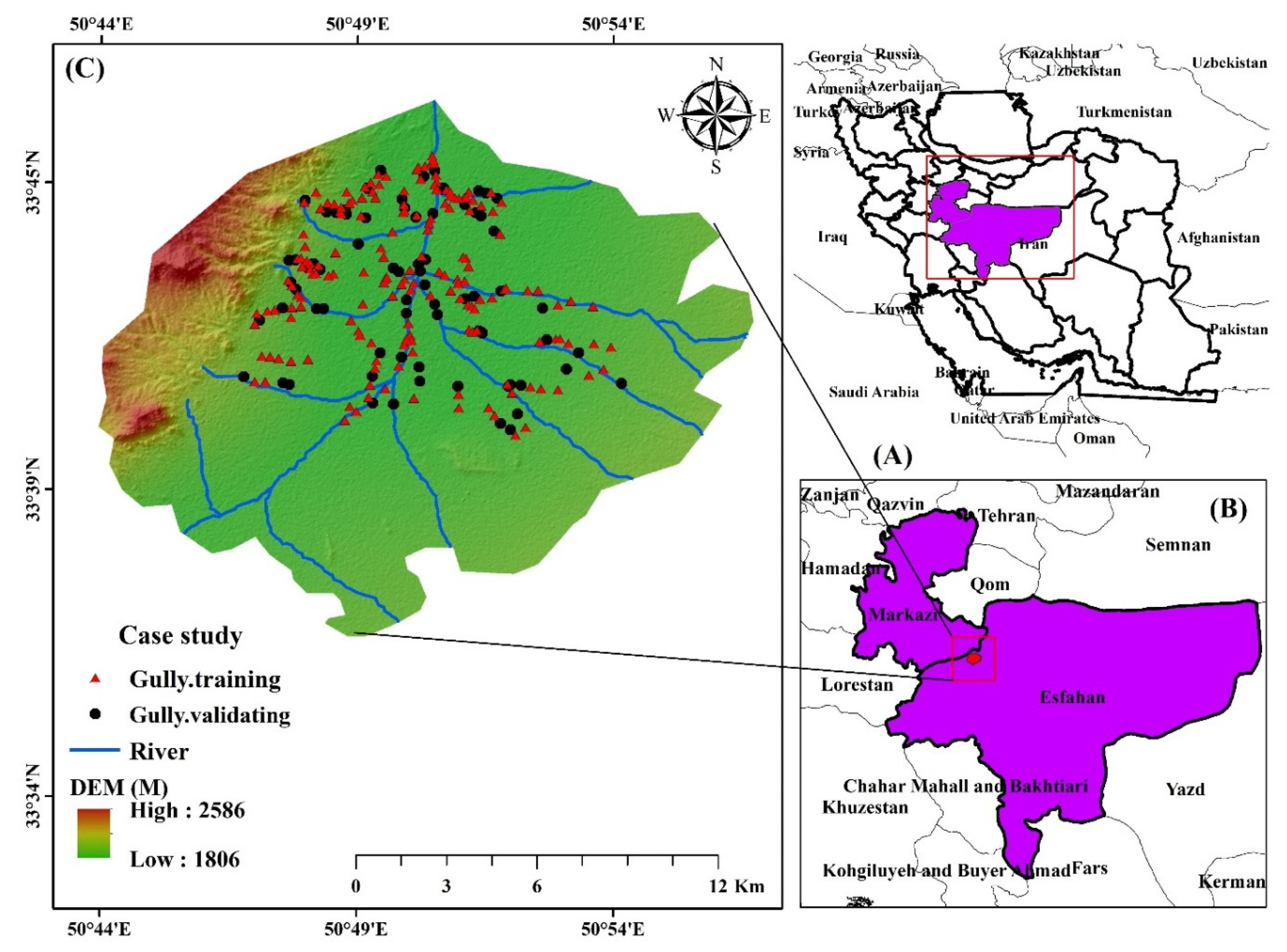
2.1. Study Area
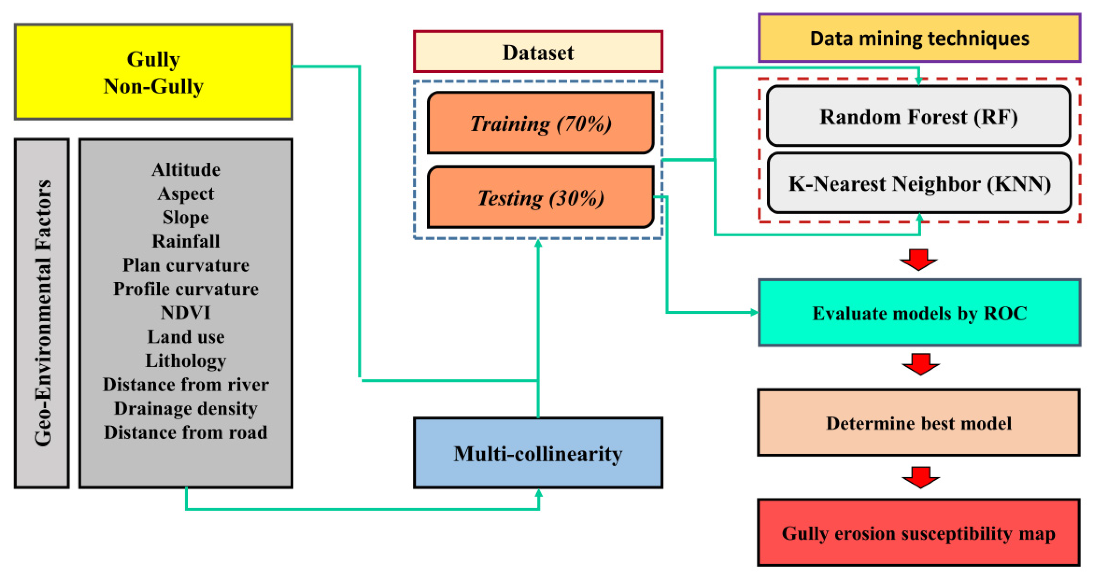
2.2. Methodology
2.2.1. Gully Dataset
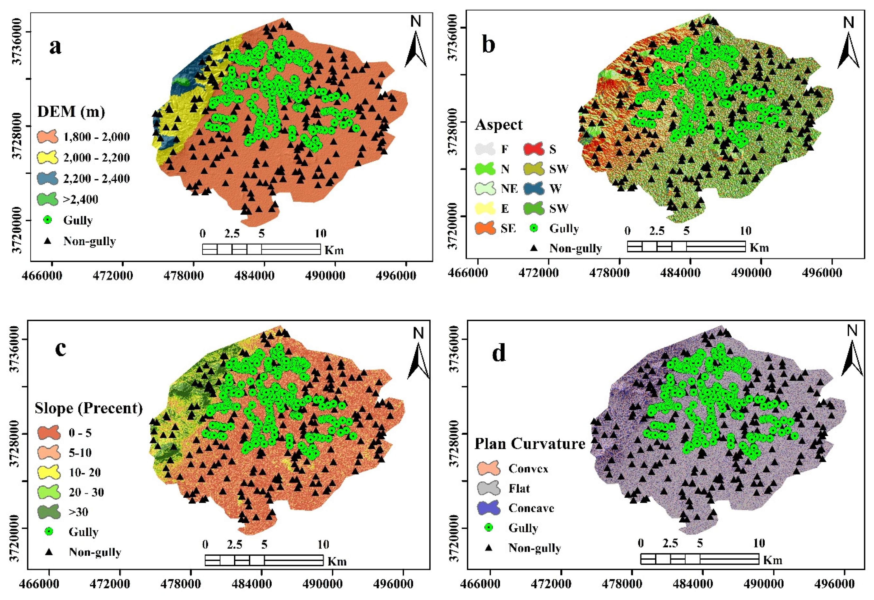
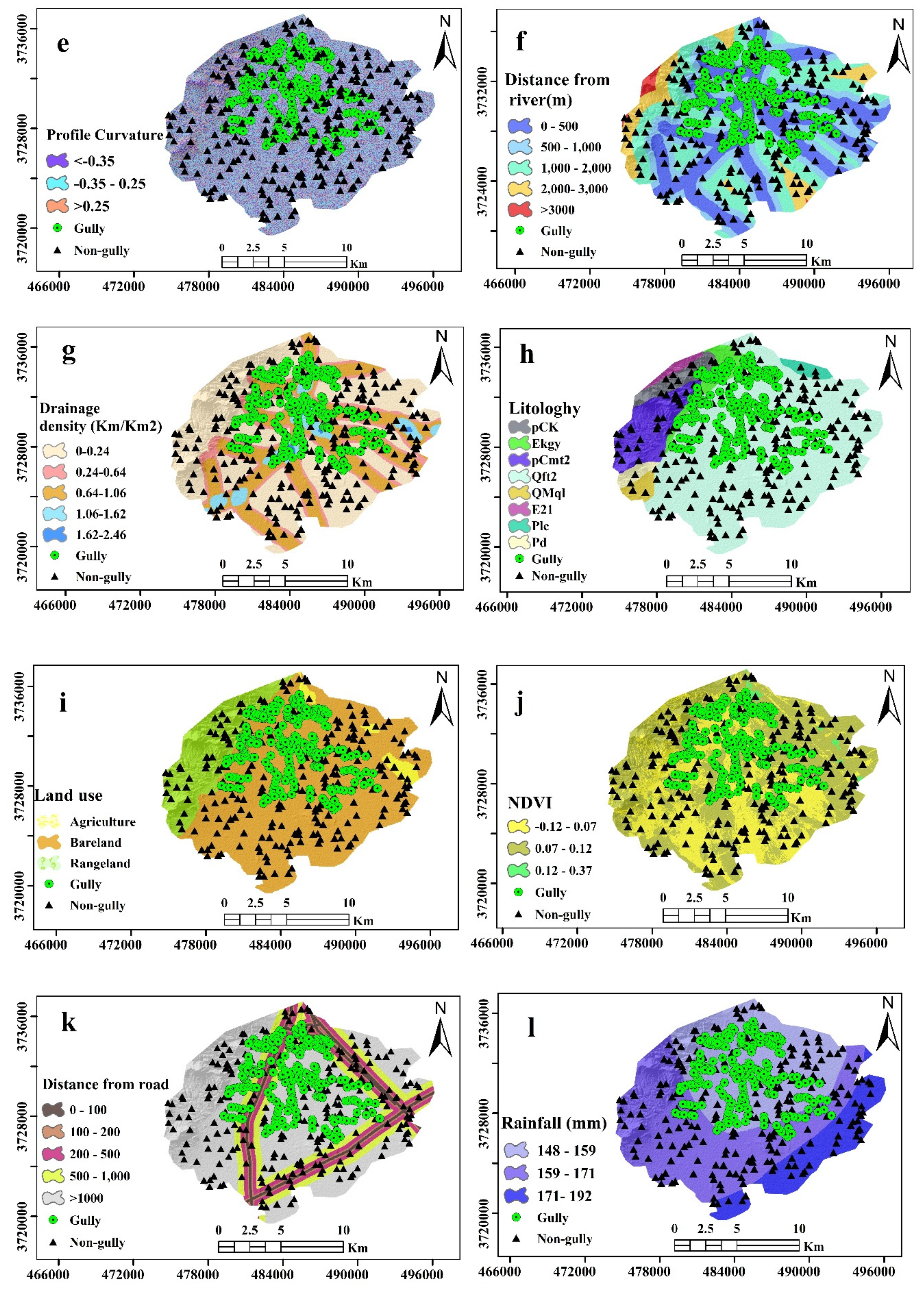
2.2.2. Gully Erosion Geo-Environmental Factors
2.2.3. Gully Erosion Susceptibility Mapping Using Data Mining Methods
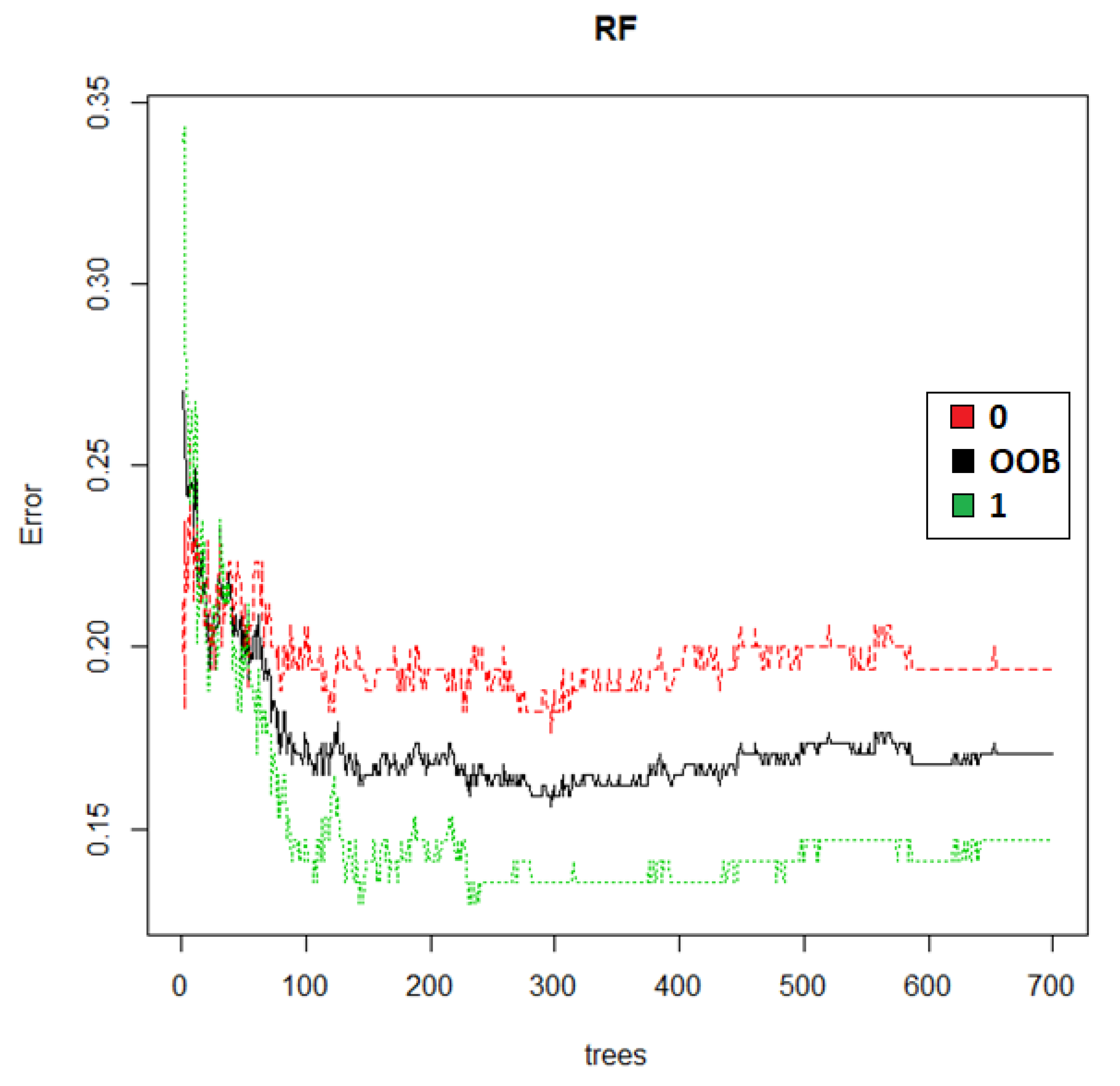
Random Forest (RF)
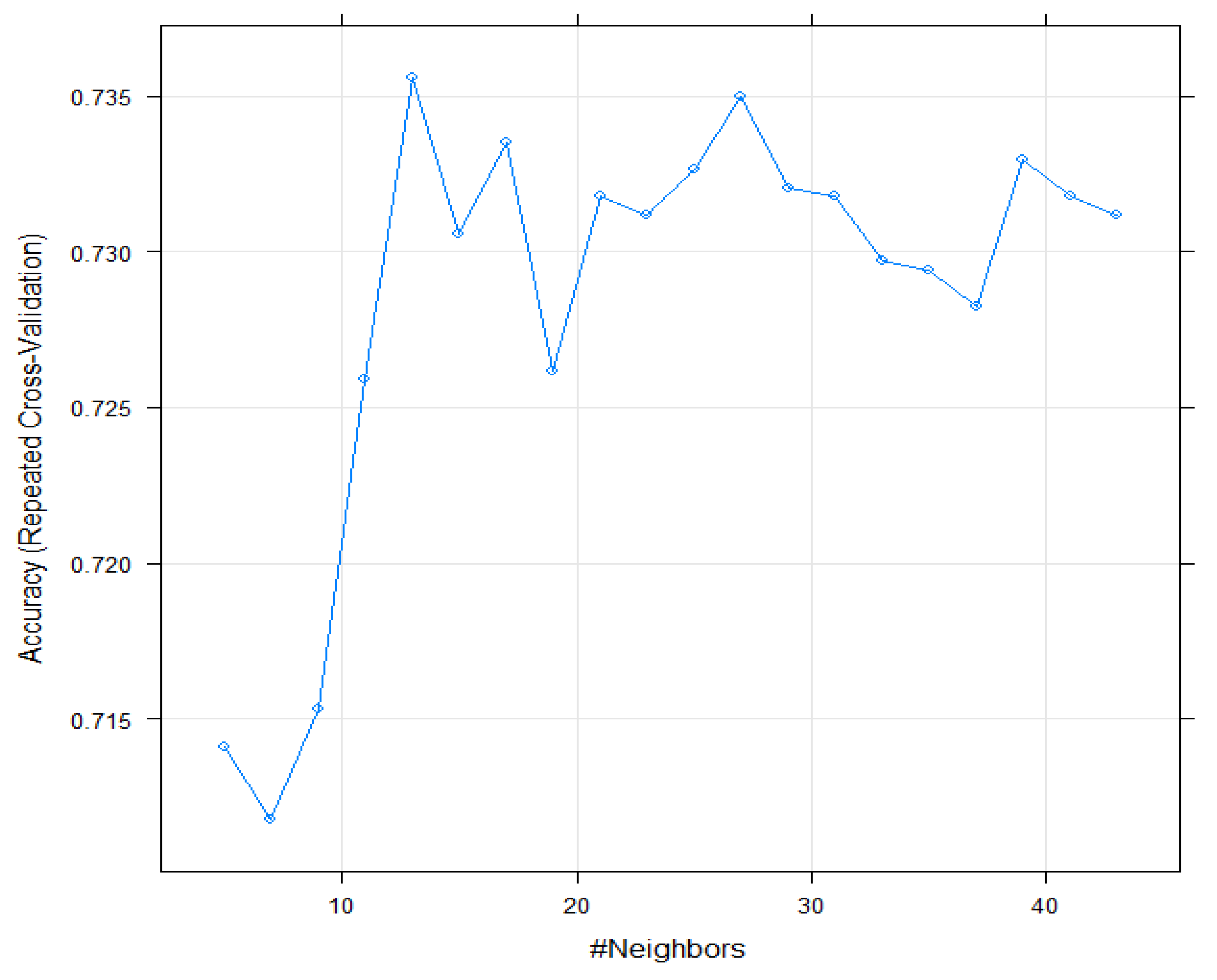
K-Nearest Neighbor (KNN)
2.2.4. Assessment of Data Mining Based Models
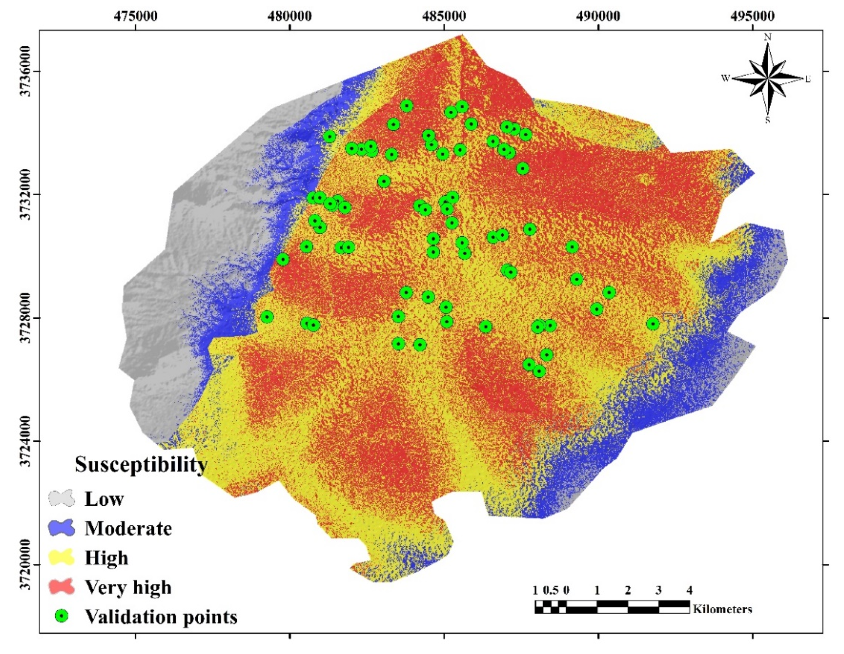
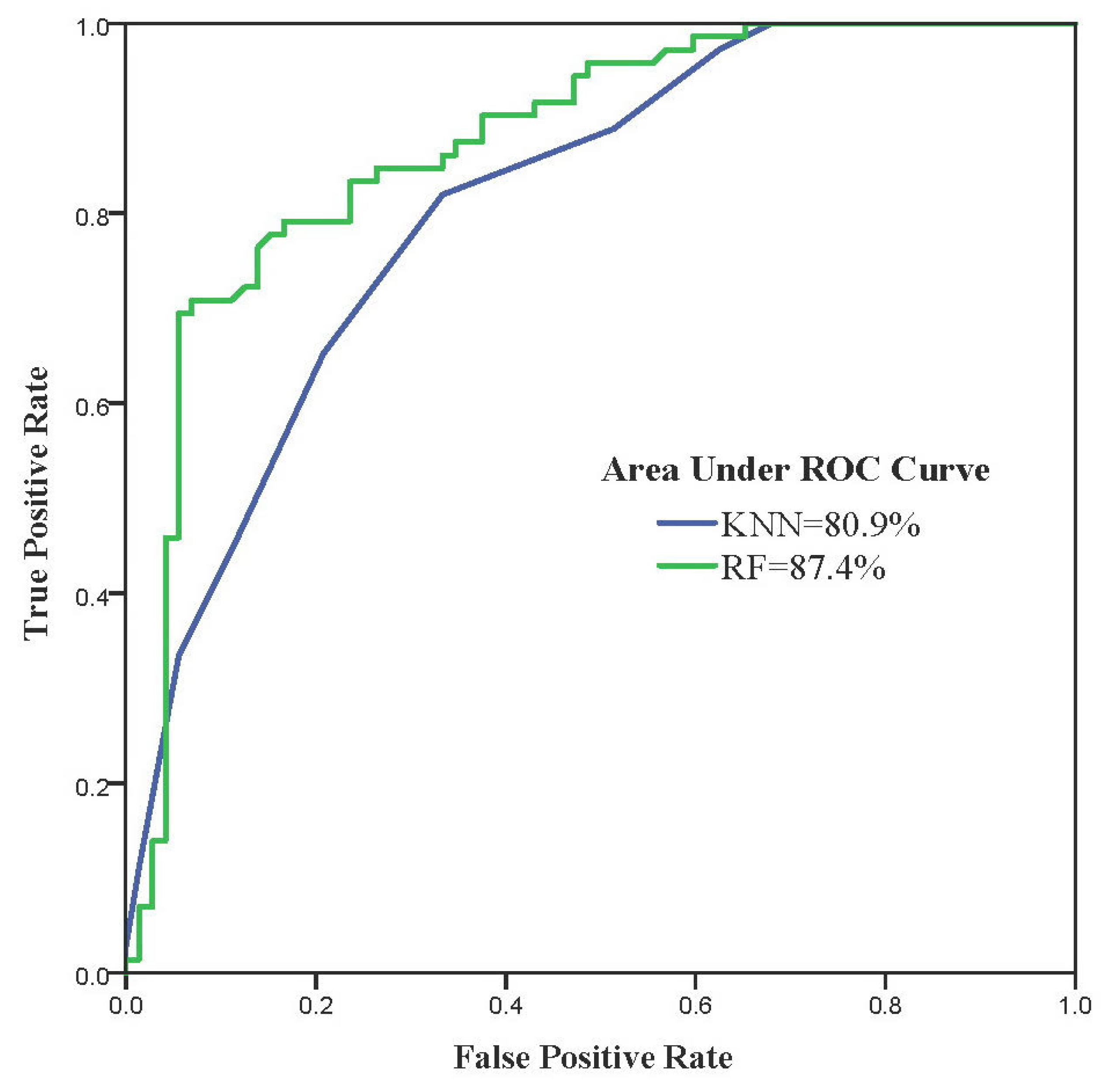
3. Results
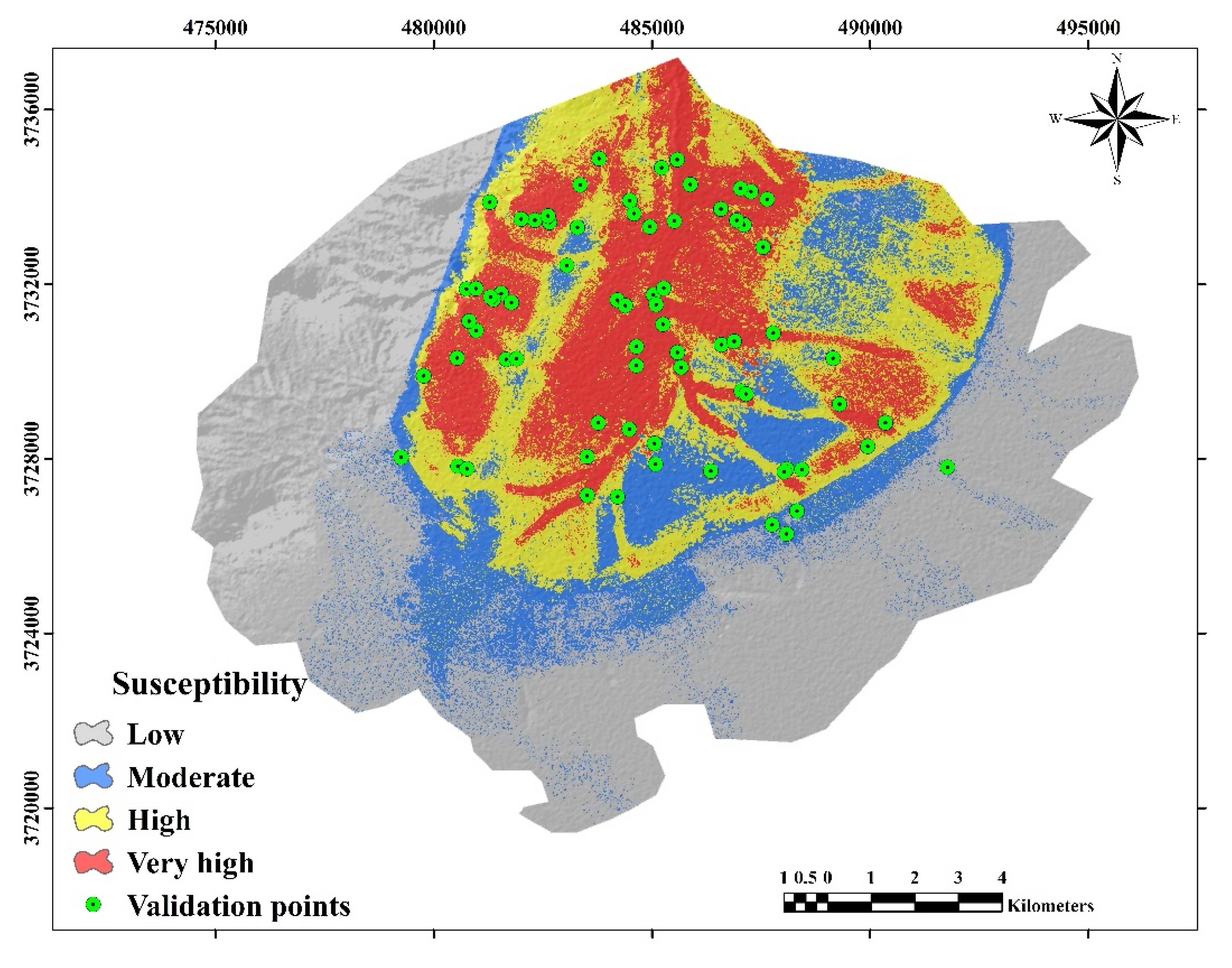
Validation of Gully Erosion Susceptibility Maps
4. Discussion
5. Conclusions
Author Contributions
Funding
Acknowledgments
Conflicts of Interest
References
- Conoscenti, C.; Angileri, S.; Cappadonia, C.; Rotigliano, E.; Agnesi, V.; Märker, M. Gully erosion susceptibility assessment by means of GIS-based logistic regression: A case of Sicily (Italy). Geomorphology 2014, 204, 399–411. [Google Scholar] [CrossRef]
- Bull, L.J.; Kirkby, M.J. (Eds.) Dryland Rivers: Hydrology and Geomorphology of Semi-Arid Channels; Wiley: Chichester, UK, 2002. [Google Scholar]
- Valentin, C.; Poesen, J.; Li, Y. Gully erosion: Impacts, factors and control. Catena 2005, 63, 132–153. [Google Scholar] [CrossRef]
- Shellberg, J.G.; Spencer, J.; Brooks, A.P.; Pietsch, T.J. Geomorphology Degradation of the Mitchell River fluvial megafan by alluvial gully erosion increased by post-European land use change, Queensland, Australia. Geomorphology 2016, 266, 105–120. [Google Scholar] [CrossRef]
- Dymond, J.R.; Herzig, A.; Basher, L.; Betts, H.D.; Marden, M.; Phillips, C.J.; Ausseil, A.-G.E.; Palmer, D.J.; Clark, M.; Roygard, J. Development of a New Zealand SedNet model for assessment of catchment-wide soil-conservation works. Geomorphology 2016, 257, 85–93. [Google Scholar] [CrossRef]
- Goodwin, N.R.; Armston, J.D.; Muir, J.; Stiller, I. Monitoring gully change: A comparison of airborne and terrestrial laser scanning using a case study from Aratula, Queensland. Geomorphology 2017, 282, 195–208. [Google Scholar] [CrossRef]
- El Maaoui, M.M.; Sfar Felfoul, M.; Boussema, M.R.; Shane, M.H. Sediment yield from irregularly shaped gullies located on the Fortuna lithologic formation in semi-arid area of Tunisia. Catena 2012, 93, 97–104. [Google Scholar] [CrossRef]
- Ionita, I.; Fullen, M.A.; Zgłobicki, W.; Poesen, J. Gully erosion as a natural and human-induced hazard. Nat. Hazards 2015, 79, 1–5. [Google Scholar] [CrossRef]
- Ibáñez, J.; Contador, J.F.L.; Schnabel, S.; Valderrama, J.M. Evaluating the influence of physical, economic and managerial factors on sheet erosion in rangelands of SW Spain by performing a sensitivity analysis on an integrated dynamic model. Sci. Total Environ. 2016, 544, 439–449. [Google Scholar] [CrossRef]
- Ekholm, P.; Lehtoranta, J. Does control of soil erosion inhibit aquatic eutrophication? J. Environ. Manag. 2012, 93, 140–146. [Google Scholar] [CrossRef]
- Moradi, H.; Avand, M.T.; Janizadeh, S. Landslide Susceptibility Survey Using Modeling Methods. In Spatial Modeling in GIS and R for Earth and Environmental Sciences, 1st ed.; Pourghasemi, H.R., Gokceoglu, C., Eds.; Elsevier: Amsterdam, The Netherlands, 2019; pp. 259–275. [Google Scholar]
- Fox, G.A.; Sheshukov, A.; Cruse, R.; Kolar, R.L.; Guertault, L.; Gesch, K.R.; Dutnell, R.C. Reservoir Sedimentation and Upstream Sediment Sources: Perspectives and Future Research Needs on Streambank and Gully Erosion. Environ. Manag. 2016, 57, 945–955. [Google Scholar] [CrossRef]
- Imeson, A.C.; Kwaad, F.J.P.M. Gully types and gully prediction. Geogr. Tydschr. 1980, 14, 430–441. [Google Scholar]
- Rijkee, P. Low-land Gully Formation in the Amhara Region, Ethiopia. Minor Master’s Thesis, Wageningen UR, Wageningen, The Netherlands, 15 December 2015. [Google Scholar]
- Barnes, N.; Luffman, I.; Nandi, A. Gully erosion and freeze-thaw processes in clay-rich soils, northeast Tennessee, USA. GeoResJ 2016, 9–12, 67–76. [Google Scholar] [CrossRef]
- Luffman, I.E.; Nandi, A.; Spiegel, T. Gully morphology, hillslope erosion, and precipitation characteristics in the Appalachian Valley and Ridge province, southeastern USA. Catena 2015, 133, 221–232. [Google Scholar] [CrossRef]
- Ollobarren, P.; Capra, A.; Gelsomino, A.; La Spada, C. Effects of ephemeral gully erosion on soil degradation in a cultivated area in Sicily (Italy). Catena 2016, 145, 334–345. [Google Scholar] [CrossRef]
- Poesen, J. Gully typology and gully control measures in the European Loess Belt. In Farm Land Erosion in Temperate Plains Environments and Hills; Wicherek, S., Ed.; Elsevier Science Publishers: Amsterdam, The Netherlands, 1993; pp. 221–239. [Google Scholar]
- Poesen, J.; Vandekerckhove, L.; Nachtergaele, J.; Oostwoud Wijdenes, D.J.; Verstraeten, G.; van Wesemael, B. Gully erosion in dryland environments. In Dryland Rivers: Hydrology and Geomorphology of Semi-Arid Channels; Bull, L.J., Kirkby, M.J., Eds.; Wiley: Chichester, UK, 2002; pp. 229–262. [Google Scholar]
- Nazari Samani, A.; Ahmadi, H.; Jafari, M.; Boggs, G.; Ghoddousi, J.; Malekian, A. Geomorphic threshold conditions for gully erosion in Southwestern Iran (Boushehr-Samal watershed). J. Asian Earth Sci. 2009, 35, 180–189. [Google Scholar] [CrossRef]
- McCloskey, G.L.; Wasson, R.J.; Boggs, G.S.; Douglas, M. Timing and causes of gully erosion in the riparian zone of the semi-arid tropical Victoria River, Australia: Management implications. Geomorphology 2016. [Google Scholar] [CrossRef]
- Gómez-Gutiérrez, Á.; Conoscenti, C.; Angileri, S.E.; Rotigliano, E.; Schnabel, S. Using topographical attributes to evaluate gully erosion proneness (susceptibility) in two mediterranean basins: Advantages and limitations. Nat. Hazards 2015, 79, 291–314. [Google Scholar] [CrossRef]
- Chaplot, V.; Coadou le Brozec, E.; Silvera, N.; Valentin, C. Spatial and temporal assessment of linear erosion in catchments under sloping lands of northern Laos. Catena 2005, 63, 167–184. [Google Scholar] [CrossRef]
- Conoscenti, C.; Angileri, S.; Cappadonia, C.; Rotigliano, E.; Agnesi, V.; Märker, M. A GIS-based approach for gully erosion susceptibility modelling: A test in Sicily, Italy. Environ. Earth Sci. 2013, 70, 1179–1195. [Google Scholar] [CrossRef]
- Lucà, F.; Conforti, M.; Robustelli, G. Comparison of GIS-based gullying susceptibility mapping using bivariate and multivariate statistics: Northern Calabria, South Italy. Geomorphology 2011, 134, 297–308. [Google Scholar] [CrossRef]
- Kornejady, A.; Ownegh, M.; Bahremand, A. Landslide susceptibility assessment using maximum entropy model with two different data sampling methods. Catena 2017, 152, 144–162. [Google Scholar] [CrossRef]
- Hosseinalizadeh, M.; Kariminejad, N.; Chen, W.; Pourghasemi, H.R.; Alinejad, M.; Behbahani, A.M.; Tiefenbacher, J.P. Spatial modelling of gully headcuts using UAV data and four best-first decision classifier ensembles (BFTree, Bag-BFTree, RS-BFTree, and RF-BFTree). Geomorphology 2019, 329, 184–193. [Google Scholar] [CrossRef]
- Rahmati, O.; Haghizadeh, A.; Pourghasemi, H.R.; & Noormohamadi, F. Gully erosion susceptibility mapping: The role of GIS-based bivariate statistical models and their comparison. Nat. Hazards 2016, 82, 1231–1258. [Google Scholar] [CrossRef]
- Angileri, S.E.; Conoscenti, C.; Hochschild, V.; Märker, M.; Rotigliano, E.; Agnesi, V. Water erosion susceptibility mapping by applying Stochastic Gradient Treeboost to the Imera Meridionale River Basin (Sicily, Italy). Geomorphology 2016, 262, 61–76. [Google Scholar] [CrossRef]
- Iranian Department of Water Resources Management of Markazi Province. Available online: http://marw.ir (accessed on 15 September 2017).
- Shadfar, S.; Davoodirad, A.A.; Peyrowan, H.R. Investigation and comparing gully erosion characteristics in agriculture and rangeland land uses, case study: Robat Tork watershed. J. Watershed Eng. Manag. 2013, 4, 217–222. [Google Scholar] [CrossRef]
- Davoodi Rad, A.A. Identification and study of gully erosion in the Robat Turk watershed 2015, Iranian Administration Department of Natural Resources of Markazi Province. Project code 9003-29-29-0. Available online: http://markazi.frw.ir (accessed on 22 June 2016).
- Golkarian, A.; Naghibi, S.A.; Kalantar, B.; Pradhan, B. Groundwater potential mapping using C5.0, random forest, and multivariate adaptive regression spline models in GIS. Environ. Monit. Assess. 2018, 190. [Google Scholar] [CrossRef]
- Oh, H.-J.; Pradhan, B. Application of a neuro-fuzzy model to landslide-susceptibility mapping for shallow landslides in a tropical hilly area. Comput. Geosci. 2011, 37, 1264–1276. [Google Scholar] [CrossRef]
- Naghibi, S.A.; Ahmadi, K.; Daneshi, A. Application of Support Vector Machine, Random Forest, and Genetic Algorithm Optimized Random Forest Models in Groundwater Potential Mapping. Water. Resour. Manag. 2017, 31, 2761–2775. [Google Scholar] [CrossRef]
- Naghibi, S.A.; Moghaddam, D.D.; Kalantar, B.; Pradhan, B.; Kisi, O. A comparative assessment of GIS-based data mining models and a novel ensemble model in groundwater well potential mapping. J. Hydrol. 2017, 548, 471–483. [Google Scholar] [CrossRef]
- Cama, M.; Lombardo, L.; Conoscenti, C.; Rotigliano, E. Improving transferability strategies for debris flow susceptibility assessment: Application to the Saponara and Itala catchments (Messina, Italy). Geomorphology 2017, 288, 52–65. [Google Scholar] [CrossRef]
- Rahmati, O.; Tahmasebipour, N.; Haghizadeh, A.; Pourghasemi, H.R.; Feizizadeh, B. Evaluation of different machine learning models for predicting and mapping the susceptibility of gully erosion. Geomorphology 2017, 298, 118–137. [Google Scholar] [CrossRef]
- Zakerinejad, R.; Maerker, M. An integrated assessment of soil erosion dynamics with special emphasis on gully erosion in the Mazayjan basin, southwestern Iran. Nat. Hazards 2015, 79, 25–50. [Google Scholar] [CrossRef]
- Rahmati, O.; Tahmasebipour, N.; Haghizadeh, A.; Pourghasemi, H.R.; Feizizadeh, B. Evaluating the influence of geo-environmental factors on gully erosion in a semi-arid region of Iran: An integrated framework. Sci. Total Environ. 2017, 579, 913–927. [Google Scholar] [CrossRef] [PubMed]
- Arabameri, A.; Rezaei, K.; Pourghasemi, H.R.; Lee, S.; Yamani, M. GIS-based gully erosion susceptibility mapping: A comparison among three data-driven models and AHP knowledge-based technique. Environ. Earth Sci. 2018, 77, 1–22. [Google Scholar] [CrossRef]
- Chunxia, Z.; Linlin, G.; Dongchen, E.; & Hsingchung, C. A case study of using external DEM in insar DEM generation. Geo. Spat. Inf. Sci. 2005, 8, 14–18. [Google Scholar] [CrossRef]
- Zabihi, M.; Mirchooli, F.; Motevalli, A.; Khaledi Darvishan, A.; Pourghasemi, H.R.; Zakeri, M.A.; Sadighi, F. Spatial modelling of gully erosion in Mazandaran Province, northern Iran. Catena 2018, 161, 1–13. [Google Scholar] [CrossRef]
- Jaafari, A.; Najafi, A.; Pourghasemi, H.R.; Rezaeian, J.; Sattarian, A. GIS-based frequency ratio and index of entropy models for landslide susceptibility assessment in the Caspian forest, northern Iran. Int. J. Environ. Sci. Technol. 2014, 11, 909–926. [Google Scholar] [CrossRef]
- Yilmaz, C.; Topal, T.; Süzen, M.L. GIS-based landslide susceptibility mapping using bivariate statistical analysis in Devrek (Zonguldak-Turkey). Environ. Earth Sci. 2012, 65, 2161–2178. [Google Scholar] [CrossRef]
- Alaska Satelatite Facility. Available online: https://vertex.daac.asf.alaska.edu/# (accessed on 22 December 2010).
- Manap, M.A.; Nampak, H.; Pradhan, B.; Lee, S.; Sulaiman, W.N.A.; Ramli, M.F. Application of probabilistic-based frequency ratio model in groundwater potential mapping using remote sensing data and GIS. Arab. J. Geosci. 2014, 7, 711–724. [Google Scholar] [CrossRef]
- Pourghasemi, H.R.; Moradi, H.R.; Fatemi Aghda, S.M.; Gokceoglu, C.; Pradhan, B. GIS-based landslide susceptibility mapping with probabilistic likelihood ratio and spatial multi-criteria evaluation models (North of Tehran, Iran). Arab. J. Geosci. 2014, 7, 1857–1878. [Google Scholar] [CrossRef]
- Pourghasemi, H.R.; Kerle, N. Random forests and evidential belief function-based landslide susceptibility assessment in Western Mazandaran Province, Iran. Environ. Earth Sci. 2016, 75. [Google Scholar] [CrossRef]
- Geological Survey and Mineral Exploration Organization of Iran. 2018. Available online: https://gsi.ir/fa (accessed on 11 November 2018).
- United States Geological Survey. Available online: https://earthexplorer.usgs.gov (accessed on 25 June 2017).
- Pourghasemi, H.R.; Youse, S.; Kornejady, A.; Cerdà, A. Performance assessment of individual and ensemble data-mining techniques for gully erosion modeling. Sci. Total Environ. 2017, 609, 764–775. [Google Scholar] [CrossRef]
- Jungerius, P.D.; Matundura, J.; van de Ancker, J.A.M. Road construction and gully erosion in West Pokot, Kenya. Earth Surf. Process. Landf. 2002, 27, 1237–1247. [Google Scholar] [CrossRef]
- Nyssen, J.; Poesen, J.; Moeyersons, J.; Luyten, E.; Veyret-Picot, M.; Deckers, J.; Haile, M.; Govers, G. Impact of road building on gully erosion risk: A case study from the Northern Ethiopian Highlands. Earth Surf. Process. Landf. 2002, 27, 1267–1283. [Google Scholar] [CrossRef]
- Bhunia, G.S.; Shit, P.K.; Maiti, R. Comparison of GIS-based interpolation methods for spatial distribution of soil organic carbon (SOC). J. Saudi Soc. Agric. Sci. 2018, 17, 114–126. [Google Scholar] [CrossRef]
- Loh, W.Y. Classification and regression trees. Wiley Interdiscip. Rev. Data Min. Knowl. Discov. 2011, 1, 14–23. [Google Scholar] [CrossRef]
- Kim, J.-C.; Lee, S.; Jung, H.-S.; Lee, S. Landslide susceptibility mapping using random forest and boosted tree models in Pyeong-Chang, Korea. Geocarto Int. 2018, 33, 1000–1015. [Google Scholar] [CrossRef]
- Breiman, L. Random forests. Mach. Learn. 2001, 45, 5–32. [Google Scholar] [CrossRef]
- Micheletti, N.; Foresti, L.; Robert, S.; Leuenberger, M.; Pedrazzini, A.; Jaboyedoff, M.; Kanevski, M. Machine Learning Feature Selection Methods for Landslide Susceptibility Mapping. Math. Geosci. 2014, 46, 33–57. [Google Scholar] [CrossRef]
- Naghibi, S.A.; Moradi Dashtpagerdi, M. Evaluation of four supervised learning methods for groundwater spring potential mapping in Khalkhal region (Iran) using GIS-based features. Hydrogeol. J. 2017, 25, 169–189. [Google Scholar] [CrossRef]
- Svetnik, V.; Liaw, A.; Tong, C.; Culberson, J.C.; Sheridan, R.P.; Feuston, B.P. Random Forest: A Classification and Regression Tool for Compound Classification and QSAR Modeling. J. Chem. Inf. Model. 2003, 43, 1947–1958. [Google Scholar] [CrossRef]
- R Core Team. R: A Language and Environment for Statistical Computing. 2018. The R Project for Statistical Computing. Available online: https://www.r-project.org (accessed on 22 June 2016).
- Breiman, L. Classification and Regression Trees, 1st ed.; Routledge: New York, NY, USA, 1984. [Google Scholar] [CrossRef]
- Mitchell, T.M. Machine Learning; McGraw-Hill: New York, NY, USA, 1997. [Google Scholar]
- Betrie, G.D.; Tesfamariam, S.; Morin, K.A.; Sadiq, R. Predicting copper concentrations in acid mine drainage: A comparative analysis of five machine learning techniques. Environ. Monit. Assess. 2013, 185, 4171–4182. [Google Scholar] [CrossRef]
- Naghibi, S.A.; Vafakhah, M.; Hashemi, H.; Pradhan, B.; Alavi, S.J. Water Resources Management Through Flood Spreading Project Suitability Mapping Using Frequency Ratio, k-nearest Neighbours, and Random Forest Algorithms. Nat. Resour. Res. 2019, 1–19. [Google Scholar] [CrossRef]
- Araghinejad, S. Data-Driven Modeling: Using MATLAB® in Water Resources and Environmental Engineering; Springer: Dordrecht, The Netherlands, 2013; Volume 67. [Google Scholar] [CrossRef]
- Park, S.; Choi, C.; Kim, B.; Kim, J. Landslide susceptibility mapping using frequency ratio, analytic hierarchy process, logistic regression, and artificial neural network methods at the Inje area, Korea. Environ. Earth Sci. 2013, 68, 1443–1464. [Google Scholar] [CrossRef]
- Razandi, Y.; Pourghasemi, H.R.; Neisani, N.S.; Rahmati, O. Application of analytical hierarchy process, frequency ratio, and certainty factor models for groundwater potential mapping using GIS. Earth Sci. Inform. 2015, 8, 867–883. [Google Scholar] [CrossRef]
- Yesilnacar, E.K. The Application of Computational Intelligence to Landslide Susceptibility Mapping in Turkey. Ph.D. Thesis, University of Melbourne, Melbourne, Australia, 2005. [Google Scholar]
- Kuhn, M. Building predictive models in R using the caret package. J. Stat. Softw. 2008, 28, 1–26. [Google Scholar] [CrossRef]
- Jenks, G.F. The Data Model Concept in Statistical Mapping. Int. Yearb. Cartogr. 1967, 7, 186–190. [Google Scholar]
- Chen, W.; Pourghasemi, H.R.; Naghibi, S.A. A comparative study of landslide susceptibility maps produced using support vector machine with different kernel functions and entropy data mining models in China. Bull. Eng. Geol. Environ. 2018, 77, 647–664. [Google Scholar] [CrossRef]
- Lee, S.; Kim, J.-C.; Jung, H.-S.; Lee, M.J.; Lee, S. Spatial prediction of flood susceptibility using random-forest and boosted-tree models in Seoul metropolitan city, Korea. Geomat. Nat. Haz. Risk. 2017, 8, 1185–1203. [Google Scholar] [CrossRef]
- Nicodemus, K.K. Letter to the Editor: On the stability and ranking of predictors from random forest variable importance measures. Brief. Bioinform. 2011, 12, 369–373. [Google Scholar] [CrossRef]
- Rizeei, H.M.; Pradhan, B.; Saharkhiz, M.A. An integrated fluvial and flash pluvial model using 2D high-resolution sub-grid and particle swarm optimization-based random forest approaches in GIS. Complex Intell. Syst. 2019, 5, 283–302. [Google Scholar] [CrossRef]
- Zhang, X.; Fan, J.; Liu, Q.; Xiong, D. The contribution of gully erosion to total sediment production in a small watershed in Southwest China. Phys. Geogr. 2018, 39, 246–263. [Google Scholar] [CrossRef]
- Garosi, Y.; Sheklabadi, M.; Conoscenti, C.; Pourghasemi, H.R.; Van Oost, K. Assessing the performance of GIS-based machine learning models with different accuracy measures for determining susceptibility to gully erosion. Sci. Total Environ. 2019, 664, 1117–1132. [Google Scholar] [CrossRef]
- Kantardzic, M. Data Mining: Concepts, Models, Methods, and Algorithms, 2nd ed.; Wiley-IEEE Press: Hoboken, NJ, USA, 2011. [Google Scholar]
- Naghibi, S.A.; Pourghasemi, H.R.; Abbaspour, K. A comparison between ten advanced and soft computing models for groundwater qanat potential assessment in Iran using R and GIS. Theor. Appl. Climatol. 2018, 131, 967–984. [Google Scholar] [CrossRef]
- Kinnell, P.I.A. Raindrop-impact-induced erosion processes and prediction: A review. Hydrol. Process. 2005, 19, 2815–2844. [Google Scholar] [CrossRef]
- Van Dijk, A.I.J.M.; Bruijnzeel, L.A.; Rosewell, C.J. Rainfall intensity–kinetic energy relationships: A critical literature appraisal. J. Hydrol. 2002, 261, 1–23. [Google Scholar] [CrossRef]
- Endale, D.M.; Fisher, D.S.; Steiner, J.L. Hydrology of a zero-order Southern Piedmont watershed through 45 years of changing agricultural land use. Part 1. Monthly and seasonal rainfall-runoff relationships. J. Hydrol. 2006, 316, 1–12. [Google Scholar] [CrossRef]
- Azareh, A.; Rahmati, O.; Rafiei-Sardooi, E.; Sankey, J.B.; Lee, S.; Shahabi, H.; Ahmad, B.B. Modelling gully-erosion susceptibility in a semi-arid region, Iran: Investigation of applicability of certainty factor and maximum entropy models. Sci. Total Environ. 2019, 655, 684–696. [Google Scholar] [CrossRef]
- Dube, F.; Nhapi, I.; Murwira, A.; Gumindoga, W.; Goldin, J.; Mashauri, D.A. Potential of weight of evidence modelling for gully erosion hazard assessment in Mbire District – Zimbabwe. Phys. Chem. Earth 2014, 67–69, 145–152. [Google Scholar] [CrossRef]


| Row | Code | Lithology | Geological Age |
|---|---|---|---|
| 1 | Qft2 | Low level pediment fan and valley terrace deposits | Quaternary |
| 2 | Plc | Polymictic conglomerate and sandstone | Pliocene |
| 3 | pCk | Dull green grey salty shales with subordinate intercalation of quartzitic sandstone (KAHAR FM; Morad series and Kalmard Formation) | Pre-Cambrian |
| 4 | Ekgy | Gypsum | Late Eocene |
| 5 | E2l | Nummulitic limestone | Eocene |
| 6 | pCmt2 | Low - grade, regional metamorphic rocks (Green Schist Facies) | Pre-Cambrian |
| 7 | OMql | Massive to thick - bedded reefal limestone | Oligocene-Miocene |
| 8 | Pd | Red sandstone and shale with subordinate sandy limestone (Dorud Formation) | Permian |
| Variable | Importance | |
|---|---|---|
| KNN | RF | |
| Rainfall | 100.00 | 48.74 |
| Altitude | 74.35 | 30.46 |
| Distance from rivers | 50.64 | 14.95 |
| Drainage density | 30.11 | 6.40 |
| Distance from road | 19.39 | 18.36 |
| Land use | 17.56 | 2.18 |
| NDVI | 5.66 | 8.92 |
| Slope | 5.63 | 6.32 |
| Lithology | 4.54 | 4.07 |
| Profile curvature | 1.23 | 2.70 |
| Slope aspect | 0.92 | 4.82 |
| Plan curvature | 0.00 | 4.94 |
| Observation | Predicted | Class Error | |
|---|---|---|---|
| 0 | 1 | ||
| 0 | 137 | 33 | 0.1941 |
| 1 | 25 | 145 | 0.1470 |
| Node Size | mtry | Trees | Best Tree |
|---|---|---|---|
| 5 | 5 | 700 | 235 |
| GPM Zones | RF | KNN | ||
|---|---|---|---|---|
| Range | Area% | Range | Area% | |
| Low | <0.217 | 46.42 | <0.2 | 13.23 |
| Moderate | 0.217–0.45 | 15.42 | 0.2–0.5 | 10.83 |
| High | 0.45–0.677 | 19.99 | 0.5–0.8 | 42.16 |
| Very high | >0.677 | 18.18 | >0.8 | 33.78 |
© 2019 by the authors. Licensee MDPI, Basel, Switzerland. This article is an open access article distributed under the terms and conditions of the Creative Commons Attribution (CC BY) license (http://creativecommons.org/licenses/by/4.0/).
Share and Cite
Avand, M.; Janizadeh, S.; Naghibi, S.A.; Pourghasemi, H.R.; Khosrobeigi Bozchaloei, S.; Blaschke, T. A Comparative Assessment of Random Forest and k-Nearest Neighbor Classifiers for Gully Erosion Susceptibility Mapping. Water 2019, 11, 2076. https://doi.org/10.3390/w11102076
Avand M, Janizadeh S, Naghibi SA, Pourghasemi HR, Khosrobeigi Bozchaloei S, Blaschke T. A Comparative Assessment of Random Forest and k-Nearest Neighbor Classifiers for Gully Erosion Susceptibility Mapping. Water. 2019; 11(10):2076. https://doi.org/10.3390/w11102076
Chicago/Turabian StyleAvand, Mohammadtaghi, Saeid Janizadeh, Seyed Amir Naghibi, Hamid Reza Pourghasemi, Saeid Khosrobeigi Bozchaloei, and Thomas Blaschke. 2019. "A Comparative Assessment of Random Forest and k-Nearest Neighbor Classifiers for Gully Erosion Susceptibility Mapping" Water 11, no. 10: 2076. https://doi.org/10.3390/w11102076
APA StyleAvand, M., Janizadeh, S., Naghibi, S. A., Pourghasemi, H. R., Khosrobeigi Bozchaloei, S., & Blaschke, T. (2019). A Comparative Assessment of Random Forest and k-Nearest Neighbor Classifiers for Gully Erosion Susceptibility Mapping. Water, 11(10), 2076. https://doi.org/10.3390/w11102076