Developing Hydro-Meteorological Thresholds for Shallow Landslide Initiation and Early Warning

Abstract

Consistent relations between shallow landslide initiation and associated rainfall characteristics remain difficult to identify, due largely to the complex hydrological and geological processes causing slopes to be predisposed to failure and those processes that subsequently trigger failures. Considering the importance of hillslope hydrology for rainfall-induced landsliding, we develop and test a method for identifying hybrid hydro-meteorological thresholds to assess landslide initiation potential. We outline a series of steps for using a landslide inventory in combination with triggering rainfall and antecedent wetness to identify empirical thresholds that can inform landslide early warning systems. The method is semi-automated but remains flexible enough to allow threshold developers to consider data inputs and various performance metrics with different priorities for balancing failed versus false alarms. We demonstrate the utility of our approach for two monitoring sites near Seattle, Washington and in Portland, Oregon, USA, to develop daily bilinear thresholds within a two-dimensional parameter space, which rely on accurate 24 h forecasts, measured recent rainfall and in situ soil saturation. Although there were no prior landslide thresholds for Portland, our new hybrid threshold for the Seattle area outperforms established rainfall-only thresholds for the same region. Introducing subsurface hydrologic monitoring into landslide initiation thresholds has the potential to greatly improve early warning capabilities and help reduce losses.

1. Introduction

Established approaches for identifying landslide initiation thresholds and early warning criteria have relied largely on deriving empirical relations between rainfall characteristics and past landslide occurrence [1,2,3,4,5,6,7,8]. These approaches typically provide easy-to-interpret graphs that can be used with real-time rainfall monitoring and forecasts to assess the potential for widespread shallow landsliding. However, it is increasingly recognized that these approaches may be limited because they do not account for the hydrologic processes that govern landslide initiation. In response, there have been attempts to incorporate the antecedent wetness through computations with cumulative rainfall prior to the triggering storm event [8,9,10,11,12,13] or more sophisticated physics-based modeling of infiltration processes [14,15,16,17]. In this spirit, Bogaard and Greco [18] proposed the cause-trigger conceptual framework to develop hydro-meteorological thresholds that combine the antecedent factors that cause hillslopes to be predisposed to failure and the actual trigger associated with landslide initiation. In parallel, Mirus and others [19] present a proof-of-concept for the approach by demonstrating that established rainfall-only thresholds for the Seattle area, Washington, USA, which use 3-day recent rainfall and 15-day antecedent rainfall variables [12,20], are significantly improved by merely replacing antecedent rainfall with average soil saturation measured over the same interval. This specific approach accounts for both the hydrologic cause and the recent rainfall trigger, but there are many possible formulations for such hydro-meteorological thresholds with different variables and timescales.

Identifying this type of threshold for landslide initiation requires determining the most suitable combination of input variables and corresponding timescales and defining the format of the threshold equation itself. The number of state variables defines the dimension of the landslide threshold space. For example, a threshold that relies on two variables exists in a two-dimensional (2D) parameter space and is defined by a line. Although it would be possible to use three variables to define a threshold space with a three-dimensional surface, or other multidimensional thresholds with even more variables, the parsimonious 2D approach accommodates independent variables to capture both the antecedent cause and recent triggering components of landslide initiation potential. Furthermore, lines on a 2D plot are easy to interpret graphically by a wide range of audiences. Traditional rainfall-only approaches typically define 2D threshold spaces by plotting average rainfall intensity against storm duration [1,6] or cumulative precipitation during some specified recent and/or antecedent duration [12,20], then identify a linear or exponential threshold equation relating the two variables. However, these may not be appropriate for very short or very long events and reflect the inherent redundancy in comparing both intensity and duration [18]. In contrast, separating the cause and trigger potentially avoids state variables and timescales with overlapping information [18,19].

Prior thresholds that are consistent with the cause-trigger concept have employed 2D parameter spaces with one threshold variable on the x-axis to represent water storage (e.g., antecedent moisture) and the other variable on the y-axis to represent water input (e.g., rainfall depth) [9,10,19,21]. Selection of timescales for the two variables requires identification of the factors relevant to the antecedent cause and distinguishing those from the triggering event, which may be difficult to determine since both contribute to landslide initiation. A useful threshold can ensure these conditions will be met when clusters of landslide events are well separated from most non-landslide events within the threshold space defined by the two variables. The degree of clustering may depend on the selected timescales for the recent and antecedent variables. Measured variables reflecting subsurface hydrologic conditions such as pore-water pressure, water table depth, or soil moisture define the underlying factors that actually cause and trigger landsliding [22,23,24,25], which is reflected in various approaches that attempt to use rainfall to calculate subsurface hydrological conditions [9,10,11,12,13,14,15,16,17]. However, it is difficult to quantify the non-linear response of soil moisture to antecedent rainfall. In contrast, one major advantage of using rainfall instead of subsurface state variables as the recent triggering variable is that this approach facilitates integration of meteorological forecasts to allow greater lead-time in advance of landsliding. Therefore, we explore the development of hybrid hydro-meteorological thresholds for a given geographic area to inform landslide early warning systems.

2. Materials and Methods

We seek to streamline the complex process of identifying and optimizing hydro-meteorological thresholds and propose a systematic method that still allows the user some flexibility to constrain the desired time-scale and proportion of failed to false alarms. Our method uses an iterative process with user input at key decision stages to test many possible landslide thresholds (Figure 1). Whereas thresholds are optimized objectively with receiver operating characteristics (ROC), different threshold variables and skill statistics used for optimization can influence the utility of said threshold for a landslide alert system, depending on end-user objectives, requirements and data availability. To demonstrate the implementation and utility of our approach we leverage landslide inventories and telemetered near-real-time measurements of rainfall and hillslope hydrologic response for two landslide prone areas in the Pacific Northwest of the United States: The Seattle-Everett railway, Washington [24] and the City of Portland, Oregon [25]. In both Seattle and Portland, shallow translational slope failures are a common and destructive form of landslide hazard during the winter rainy season (November–April), but uncommon during the drier half of the year (May–October).

2.1. Field Monitoring Sites

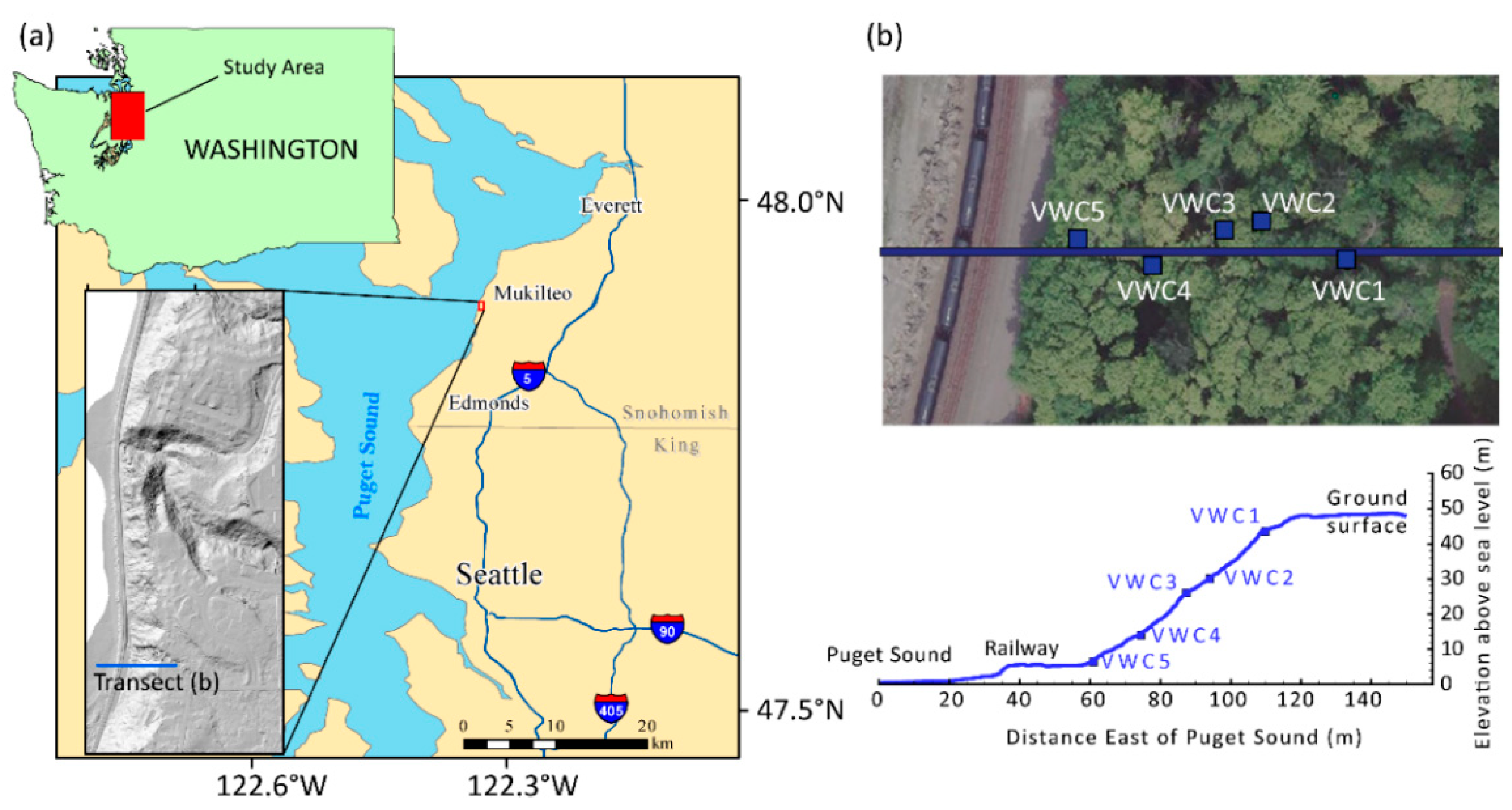
The Seattle-Everett railway monitoring site (Figure 2) and the Portland Hills monitoring site (Figure 3) are both located in steep, densely forested terrain with a mantle of colluvial soil that is typically involved in shallow slope failures [24,25]. Mean annual precipitation of around 889 mm along the Seattle-Everett railway and around 937 mm within the City of Portland, with precipitation falling mainly during the winter months of December through February in the form of rainfall or rapidly melting snow. The average slopes at the Seattle and Portland area monitoring sites are 35° and 31°, respectively. Both sites include instrumentation to measure rainfall and subsurface hydrologic response, including volumetric water content (VWC). For the Seattle area site, five sensors are installed at 1.00, 1.30, 1.00, 1.10 and 1.10 m depths in soil pits spaced at regular intervals along a 60-m long transect of a 42-m high vegetated hillslope (Figure 2). At the Portland site, 11 sensors are installed at 0.20, 0.30, 0.40, 0.50, 0.60, 0.70, 0.80, 0.90, 1.05, 1.20 and 1.30 m depths below the surface in one soil pit approximately 25 m from the hillslope crest (Figure 3).

Comprehensive monitoring for the Seattle-Everett railway site in Mukilteo began in August 2015 and our analysis uses monitoring data from 17 August 2015 to 31 May 2017 [24], during which time a total of 17 landslide-blocking events (Table S1) were recorded along the railway below the monitoring site [19,20]. Initial monitoring in the City of Portland began in 2006 November, but some breaks in the time series prevent the rainfall and subsurface data from being used in tandem. Instead, our analysis uses monitoring data from 13 November 2009 to 23 January 2016 [25], during which time a total of 93 landslides were recorded within the City of Portland (Table S2) by the Oregon Department of Geology and Mineral Industries’ (DOGAMI) statewide landslide inventory database [26]. Further information on the two monitoring sites, including geologic site characterization, study area maps and instrument configuration can be found elsewhere [24,25]. Interactive maps of the study locations and the current rainfall and hillslope hydrologic conditions are available on the U.S. Geological Survey (USGS) Landslide Hazards Program monitoring sites for Seattle and Portland [27,28].

2.2. Data Inputs

Tipping bucket gages measure rainfall via the timing of small depth increments (i.e., 0.02 mm). Whereas rapid timing of successive bucket tips recorded in a data logger may reflect increased potential for landslide initiation, the accumulation of sufficient rainfall amounts over a fixed time or storm duration is a more intuitive consideration that can be integrated with historical and other datasets. This accumulation is the basis for determining rainfall intensity-duration thresholds for individual storms [1,2,6], defining mean intensity thresholds for a given fixed interval, such as 15-min or hourly intensities [4], or for using cumulative rainfall thresholds defined over a fixed duration, such as several days [12,14,19,20].

To develop thresholds with predictive capabilities that can provide warning in advance of elevated landslide potential, we calculate threshold variables 24 h before the time of interest. However, since the influence of rainfall forecast accuracy is beyond the scope of this study, we use retroactively measured rainfall as a proxy for accurate quantitative precipitation forecasts. Therefore, our meteorological variable represents an accumulation of recent and imminent rainfall responsible for landslide triggering, which we analyze over different numbers of days in duration to identify the appropriate timescales. For example, at time t, a 3-day timescale for our meteorological variable is calculated as the cumulative rainfall from t − 48 h through t + 24 h.

Following previous efforts [19], we use saturation at time t for the hydrologic variable, which we calculate by normalizing VWC with porosity for each probe:

$$\mathrm{Saturation}\left(\mathrm{t}\right)=\frac{\mathrm{VWC}\left(\mathrm{t}\right)}{\mathrm{porosity}}$$

(1)

where we assume that the porosity at each probe is equivalent to the maximum observed VWC that coincides with simultaneous observations of positive pore-water pressures [24,25]. Measured hydraulic properties from the Seattle area site [29] suggest this assumption regarding porosity is reasonable. We then take the average saturation over all depths and locations within each study site to calculate the antecedent saturation variable, which we again average over different numbers of days in duration to identify appropriate timescales. Averaging over a fixed duration is equivalent to applying a moving average filter to dampen high-frequency noise that might otherwise inadvertently trigger failed or false alarms.

Unlike rainfall, saturation is not readily forecasted and yet rainfall influences saturation. To avoid overlapping information between these respective meteorological trigger and hydrologic cause variables, we maintain the previously demonstrated approach for calculating antecedent saturation during the specified time interval prior to the recent rainfall accumulation [19]. For example, at time t, a 3-day timescale for our antecedent saturation variable paired with a 3-day cumulative rainfall variable (2 days prior and 1 day forecasted) is calculated as the average saturation from t − 120 h.

2.3. Threshold Formats, Variables and Timescales

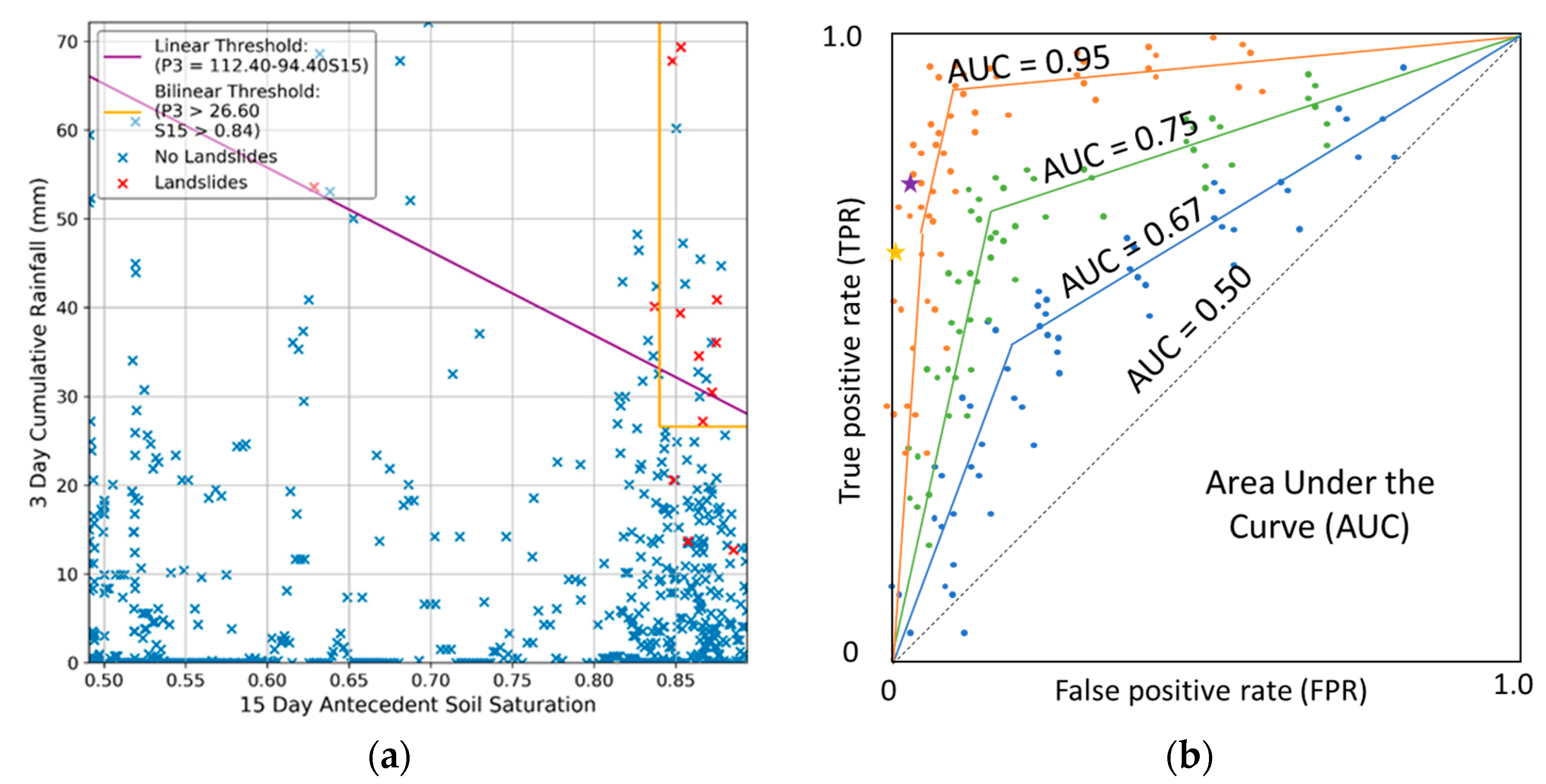
For this study, we build upon the preliminary proof-of-concept for the Seattle area, which used a 2D data plot of 3-day recent rainfall and 15-day antecedent saturation to identify thresholds using a simple linear equation optimized with the threat score statistic [19]. Landslide events clustered in the upper right corner of the threshold space, indicating that the simple linear threshold can be outperformed by alternative formats, such as bilinear thresholds (Figure 4a). Here, we systematically explore alternate timescales for both the rainfall and antecedent saturation variables, compare optimized thresholds with bilinear formats and examine the potential utility of incorporating accurate 24 h rainfall forecasts to provide greater lead-time in hazard assessments.

Previous analysis of rainfall-only thresholds for the Seattle area found modest improvements in performance using moving intervals with hourly data inputs and threshold calculations rather than daily fixed intervals [20]. However, this prior analysis relied on precise landslide timing information for the Seattle-Everett railway (Table S1), whereas the Portland inventory records only the date of landslide occurrence (Table S2). Although our monitoring records at 15-min intervals [24,25], we follow prior precedent of optimizing daily thresholds with fixed intervals [12,19] to maintain consistency with the minimum temporal resolution of our landslide inventories.

2.4. Threshold Optimization Metrics

We tested our possible threshold formulations and optimal threshold equations using ROC analysis [30,31] with different optimization metrics. First, we computed a confusion matrix, which tallies the number of: true positives (TP), which are correct predictions of landsliding; false positives (FP), which are incorrect predictions of landsliding when no landslides are reported (i.e., false alarms); true negatives (TN), which are correct predictions of no landsliding; and false negatives (FN), which are failures to predict the occurrence of landsliding (i.e., failed alarms). We calculate and evaluate thresholds using a fixed interval between 0:00–23:59 local time, so positive events are days on which one or more landslides occur (Tables S1 and S2; red ‘x’ in Figure 4a) and negative events are days when no landslides occur (blue ‘x’ in Figure 4a); true events are days on which either positive or negative events are correctly predicted by the threshold (red ‘x’ above the thresholds and blue ‘x’ below the threshold in Figure 4a) and false events are incorrect predictions (blue ‘x’ above and red ‘x’ below the thresholds). For any given threshold, we calculate the confusion matrix by examining each day in the record and determining whether the day falls under the TP, FP, TN, or FN category.

Using values from the confusion matrix, we then calculate the true positive rate (TPR) and false positive rate (FPR) metrics as:

$$\mathrm{TPR}=\mathrm{TP}/\left(\mathrm{TP}+\mathrm{FN}\right)$$

(2)

and

$$\mathrm{FPR}=\mathrm{FP}/\left(\mathrm{FP}+\mathrm{TN}\right).$$

(3)

A perfect model with no false alarms or missed alarms will produce TPR equal to unity and FPR equal to zero, but generally landslides are not perfectly predicted so there is a trade-off between increased TPR and associated increases in FPR. For example, for the bilinear threshold in Figure 4a a lower 3-day rainfall value would correctly predict a few more landslide days, but at the expense of numerous additional false alarms. This trade-off is illustrated quantitatively by the difference between the optimized linear and bilinear thresholds and hypothetical ROC curves in Figure 4b. The ROC curve plots the TPR versus FPR metrics for a suite of possible thresholds with a given format and set of axis variables. The total area under the curve (AUC) is a metric that provides insights on the overall utility of a given formulation of the threshold space, which reflects the balance between TPR and FPR for all the possible combination of values for the two threshold variables. A higher AUC indicates the formulation can achieve higher TPR relative to the associated FPR; with a perfect model, AUC is equal to unity and for a model equivalent to random guessing, the AUC is equal to one-half.

Typically, ROC curves are obtained by altering one variable that changes the threshold and performing ROC analysis on each unique threshold. Here, we depart somewhat from standard procedure by systematically altering two variables for the bilinear thresholds in combination, which results in a cluster of points within the ROC space, rather than a single unique curve. Many points may share the same FPR but display varying TPRs (or vice versa). As there is no benefit in thresholds with lower TPRs for a given FPR (or higher FPRs for a given TPR), we create the maximum (or optimal) ROC curve by maximizing TPR and masking all other less-optimal results. This maximum curve reveals the highest possible AUC value and reflects the best subset of threshold equations within a suite of thresholds for a given variable space. Subsequently, plotting the maximum ROC curves and calculating the corresponding AUC values for multiple suites of thresholds allows a comparison of the relative performance of competing threshold formulations (Figure 4b). However, ROC curves can intersect, so higher AUC does not always mean that the optimal threshold exists within that formulation of variables; this must be determined by the desired balance between TPR and FPR, among other considerations, such as lead-time needed to take effective action. To identify the most useful threshold, the developer must select a statistical metric for optimization (Figure 1).

Common statistical metrics for landslide threshold optimization include threat score, precision, true skill statistic and optimal point (or radial distance) criteria [4,7,32], which are calculated as:

$$\mathrm{Threat}\mathrm{score}=\frac{\mathrm{TP}}{\mathrm{TP}+\mathrm{FN}+\mathrm{FP}}$$

(4)

$$\mathrm{Precision}=\frac{\mathrm{TP}}{\mathrm{TP}+\mathrm{FP}}$$

(5)

$$\mathrm{True}\mathrm{Skill}\mathrm{Statistic}=\mathrm{TPR}-\mathrm{FPR}$$

(6)

$$\mathrm{Radial}\mathrm{Distance}=\sqrt{{\left(\mathrm{FPR}\right)}^2+{\left(\mathrm{TPR}-1\right)}^2}$$

(7)

For a perfect model, the threat score, precision and true skill statistic will all equal to unity, whereas the optimal point is found when radial distance from a point representing a perfect threshold is zero. Therefore, one seeks to maximize threat score, precision and true skill statistic and minimize radial distance. Since a single threshold holding the optimal value for all skill metrics is highly unlikely, the choice of a metric for optimization will determine the degree to which the resulting threshold is optimistic (i.e., averse to failed alarms) or pessimistic (i.e., averse to false alarms). When optimized with threat score and precision, landslide thresholds are typically quite pessimistic [19,32], while the true skill statistic and optimal point optimizations can result in somewhat more optimistic or balanced thresholds [7,32].

2.5. Iterative Threshold Development

We begin with an informed initial estimate of the range of appropriate threshold variables and timescales (Figure 1, step 1), which can be based on the user’s knowledge of landslide occurrence within their study area (e.g., Figure 4a). The automated analysis then tests multiple alternate threshold spaces based on user-defined discretization, which slightly alter the timescale for the x- and y-axis components. For each of the variable timescales and formulations tested, each possible threshold is evaluated by (1) calculating the confusion matrix, which is composed of the number of TP, FP, FN and TN events; (2) using the confusion matrix to calculate the TPR, FPR and other statistics (Equations (2)–(7)) for each possible threshold; (3) plotting the maximum ROC curve for each threshold formulation, which takes the highest combination of FPR and TPR from the cluster of possible points (Figure 4b); and (4) calculating the AUC for the maximum ROC curve. Based on these outputs, all the thresholds tested are automatically queried to identify which possible equation exhibits the best score, depending on the user’s preferred skill statistic.

Through testing multiple combinations of timescales for the two variables and examining the ROC curves, AUC values and calculated skill metrics, we can quantitatively define threshold accuracy and the trade-off between failed and false alarms (Figure 1, step 2), then qualitatively assess the utility and limitations of the threshold for decision making (Figure 1, decision stage). This is a rather complex decision, since in some cases higher FPR is acceptable in exchange for high TPR and in other cases it is not. Our method includes enough flexibility that the threshold developer can consult with their target audience about the appropriate trade-off between failed and false alarms. If the threshold is not sufficiently accurate to meet the user requirements, the process can be repeated (Figure 1, step 1) with different variable inputs, formulations, timescales, discretization, or skill statistics for optimization, until reaching an acceptable outcome (Figure 1, step “done”). However, it should be noted that since the process is automated, the primary influence exerted by the threshold developer is through modifying either the discretization (i.e., dictates the total number of thresholds tested per formulation), threshold formulation (i.e., equation format), or the skill statistic (i.e., criteria used for identifying the optimal threshold). Skill statistics have the greatest impact on the trade-off between failed and false alarms, followed closely by threshold formulation.

3. Results

3.1. Seattle Area Thresholds

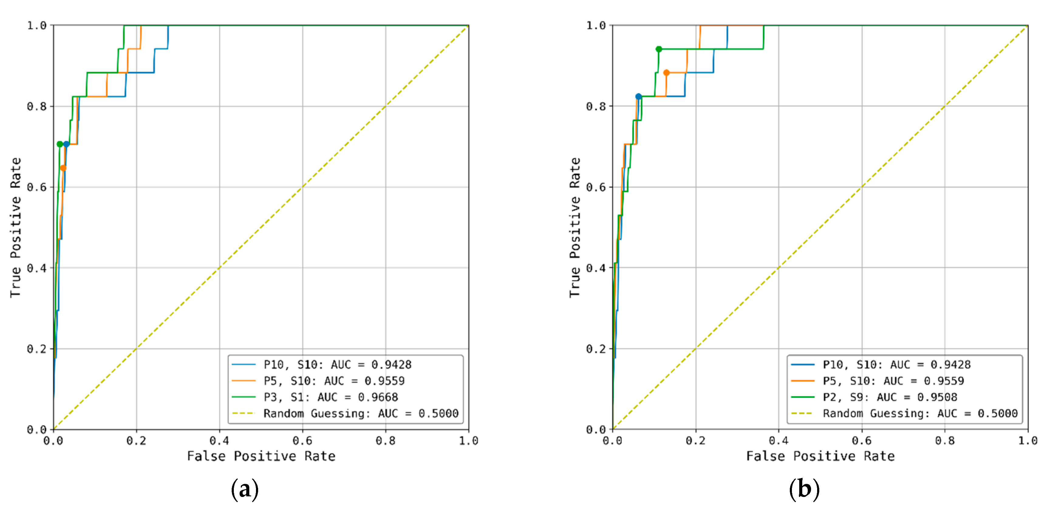
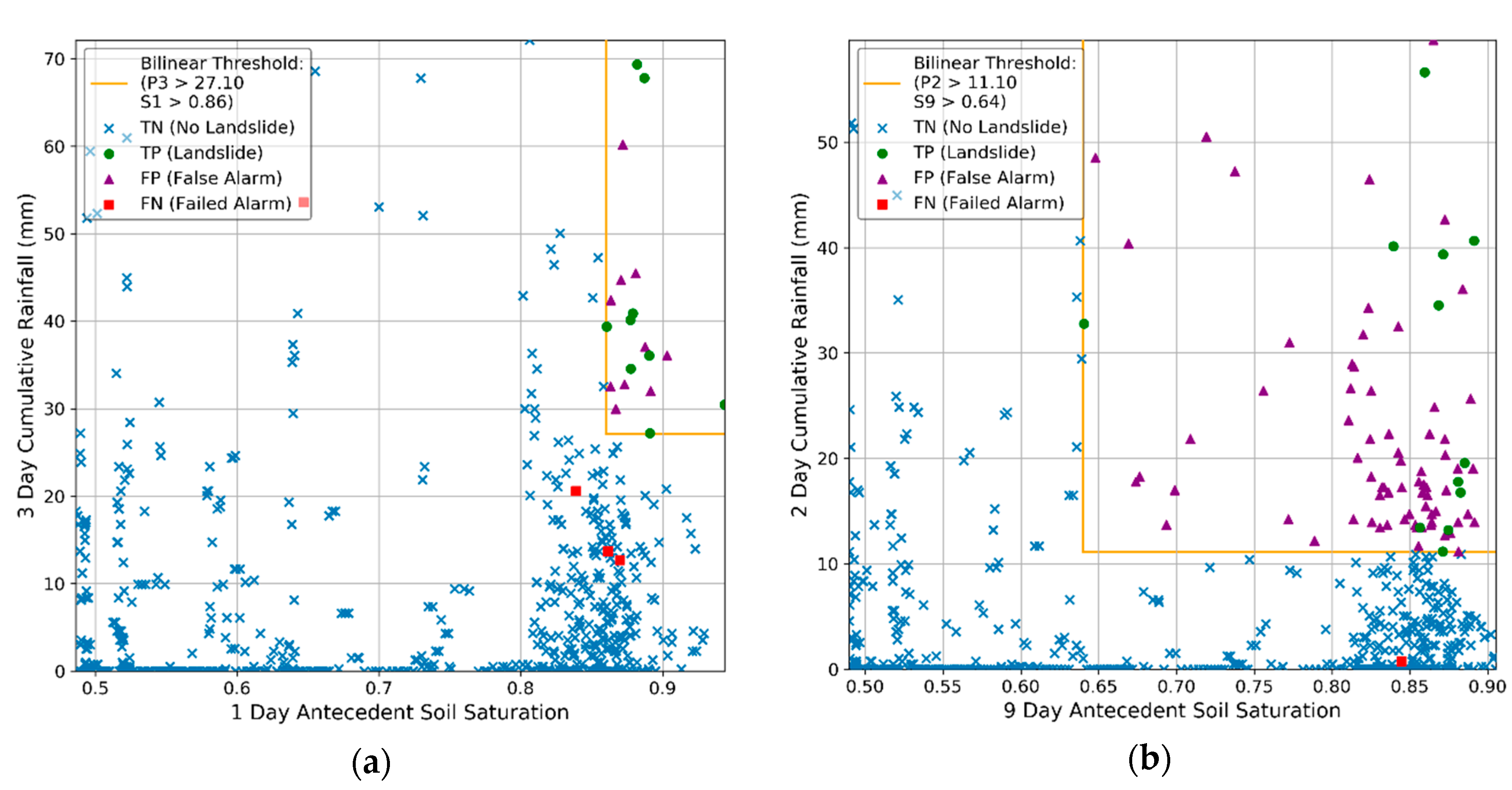
For the Seattle area dataset, we use the threat score (Equation (4)) to identify a preferred threshold space of 3-day cumulative rainfall (P3 = 1 day of imminent rainfall and 2 days of recent rainfall) with 1-day of antecedent saturation (S1), which produces the bilinear threshold with the highest threat score of 0.44, TPR of 0.71 and FPR of 0.02 (

Table 1. Selected iterations of different threshold formats for the Seattle-Everett railway, illustrating improved performance for different skill metrics. Skill metric used for optimization is in bold text, optimal threshold equation and statistics for the two different optimizations are italicized.

Timescale 1	Equation	TPR	Threat Score	Precision	True Skill Statistic	Radial Distance
P10/S10	P10 > 69.8, S10 > 0.82	0.71	0.32	0.38	0.67	0.30
P5/S10	P5 > 39.3, S10 > 0.84	0.64	0.34	0.42	0.62	0.35
P3/S1	P3 > 27.1, S1 > 0.86	0.71	0.44	0.55	0.69	0.29
P10/S10	P10 > 70.1, S10 > 0.57	0.82	0.25	0.26	0.76	0.19
P5/S10	P5 > 25.2, S10 > 0.63	0.88	0.15	0.15	0.75	0.18
P2/S9	P2 > 11.1, S9 > 0.64	0.94	0.18	0.18	0.83	0.13

¹ P10: 10-day cumulative precipitation variable; S10: 10-day antecedent saturation variable.

, Figure 5a and Figure 6a). We then repeat the process but optimize with the optimal point statistic instead (Equation (7)), to produce a very different threshold space with a 2-day rainfall variable (P2) and 9-day antecedent saturation (S9) and the lowest radial distance of 0.13, TPR of 0.94 and FPR of 0.11 (Table 1, Figure 5b and Figure 6b). The relative impact of alternative timescales and threshold values on the different skill statistics (Equations (4)–(7)) and optimal thresholds is illustrated with selected iterations from the automated ROC analysis (Table 1; Figure 5). The ROC curves generated for both the threat score and optimal point statistics show that longer timescales for the recent rainfall and antecedent saturation exhibit slightly higher AUC values for the optimal threshold format (Figure 5) indicating that the trade-off between failed alarms (FN) and false alarms (FP) is slightly more favorable at shorter timescales.

3.2. Portland Thresholds

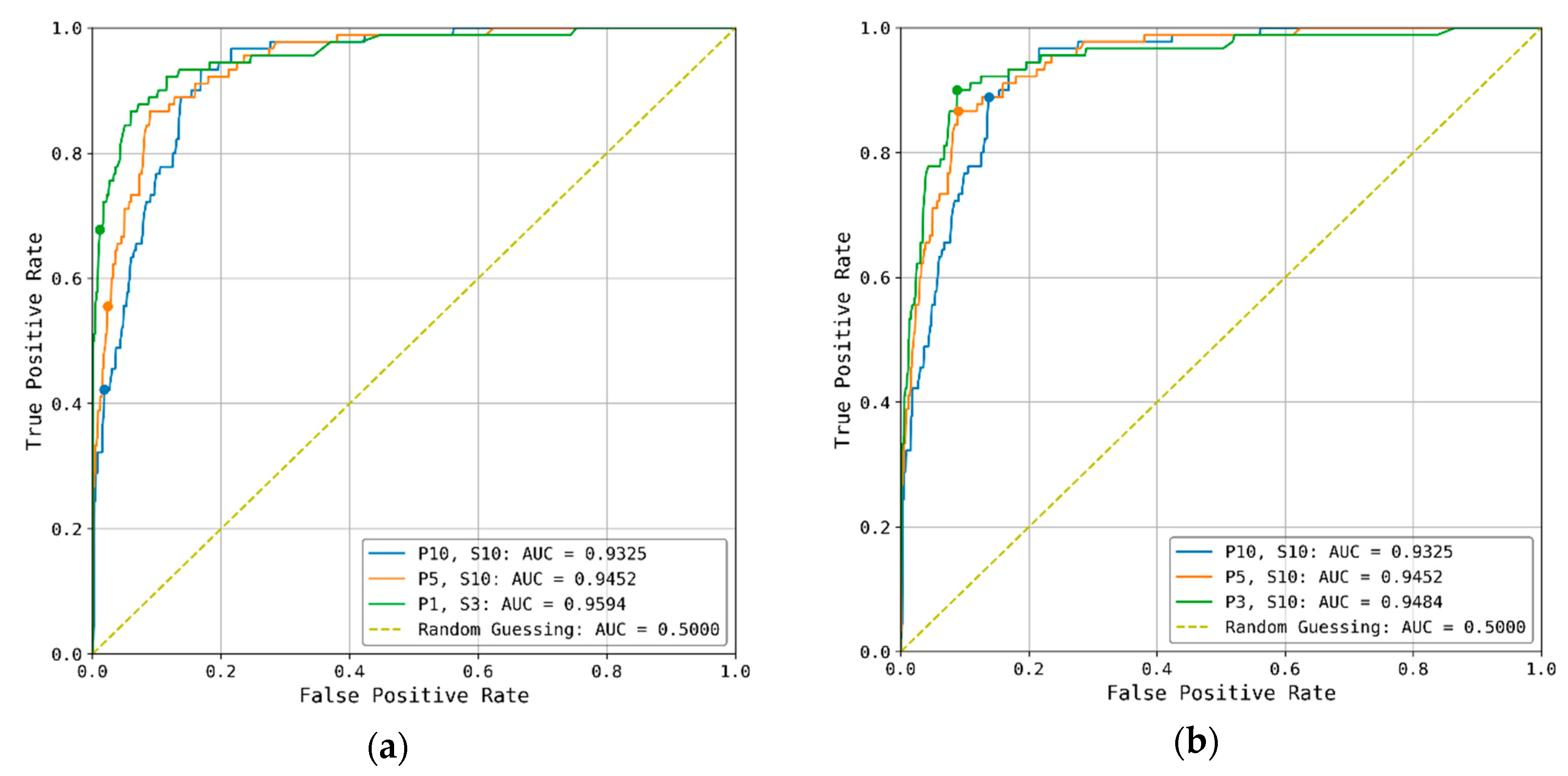
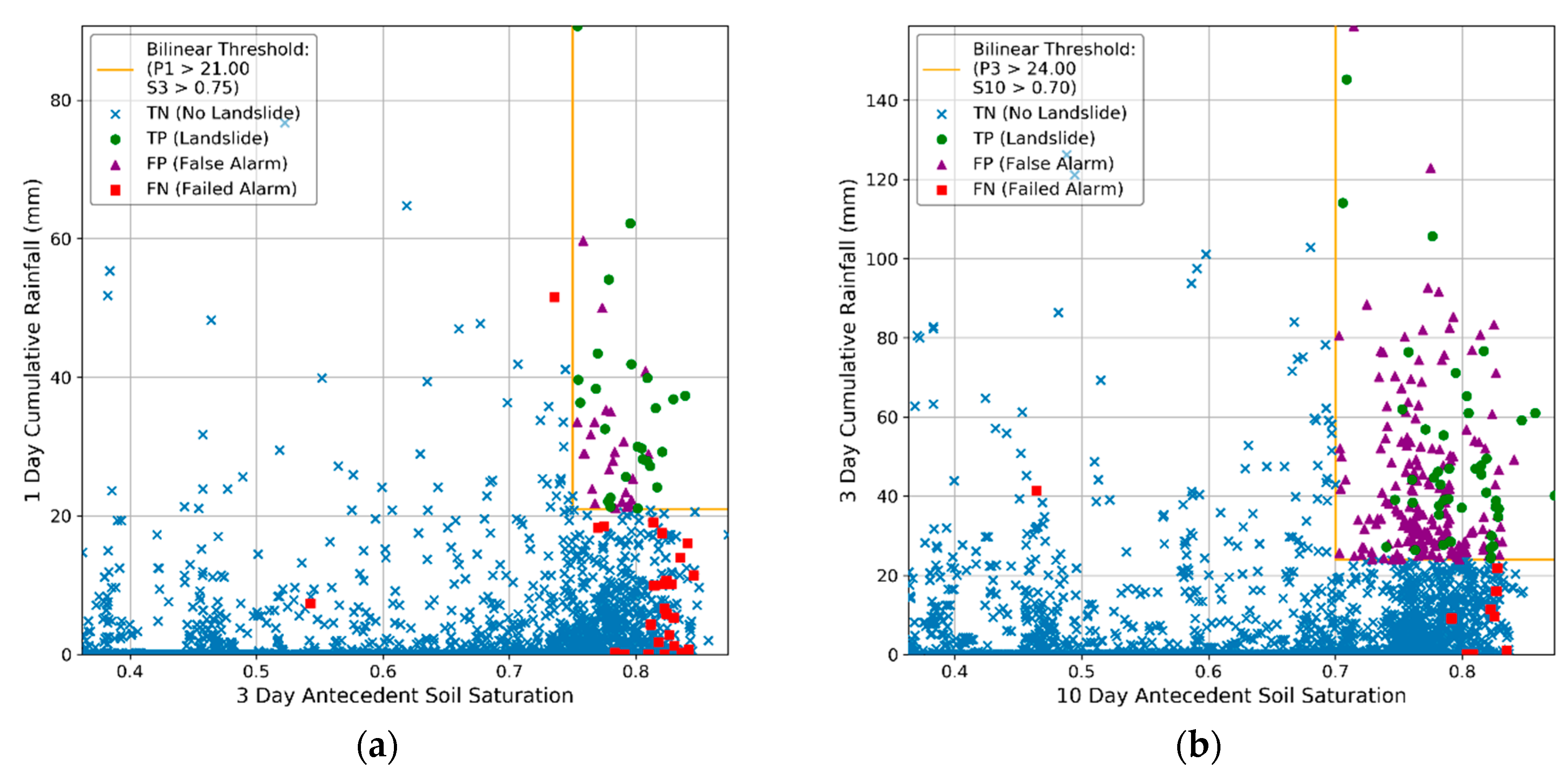
For the City of Portland dataset, we use the threat score (Equation (4)) to identify an optimal bilinear threshold with 1-day cumulative rainfall (i.e., 24 h of prediction) and 3-day antecedent saturation, which achieved a threat score of 0.68, a TPR of 0.53 and a FPR of 0.01 (Figure 7a and Figure 8a). Again, we repeat the process, but optimize with the optimal point statistic instead (Equation (7)), to produce a very different threshold space with a 3-day rainfall variable (P3) and 10-day antecedent saturation (S10) and a radial distance of 0.13, TPR of 0.90 and FPR of 0.09 (Figure 7b and Figure 8b). Similar to the results of our analysis for the Seattle area, the relative impact of alternative timescales and threshold values on the different skill statistics (Equations (4)–(7)) and optimal thresholds is illustrated with selected iterations from the automated ROC analysis (

Table 2. Selected iterations of different threshold formats for the City of Portland, illustrating improved performance for different skill metrics. Skill metric used for optimization is in bold text, optimal threshold equation and statistics for the two different optimizations are italicized.

Timescale 1	Equation	TPR	Threat Score	Precision	True Skill Statistic	Radial Distance
P10/S10	P10 > 123, S10 > 0.68	0.42	0.29	0.49	0.40	0.58
P5/S10	P5 > 76.0, S10 > 0.69	0.56	0.35	0.50	0.53	0.45
P1/S3	P3 > 21.0, S1 > 0.75	0.68	0.53	0.71	0.67	0.32
P10/S10	P10 > 61.0, S10 > 0.68	0.89	0.20	0.21	0.75	0.18
P5/S10	P5 > 39.0, S10 > 0.69	0.87	0.27	0.28	0.78	0.16
P2/S9	P2 > 24.0, S9 > 0.70	0.90	0.29	0.30	0.81	0.13

¹ P10: 10-day cumulative precipitation variable; S10: 10-day antecedent saturation variable.

; Figure 7). Although timescales are shorter for the threat score statistics, longer timescales are identified to minimize radial distance.

4. Discussion

4.1. Comparing Operational Utility of Competing Thresholds

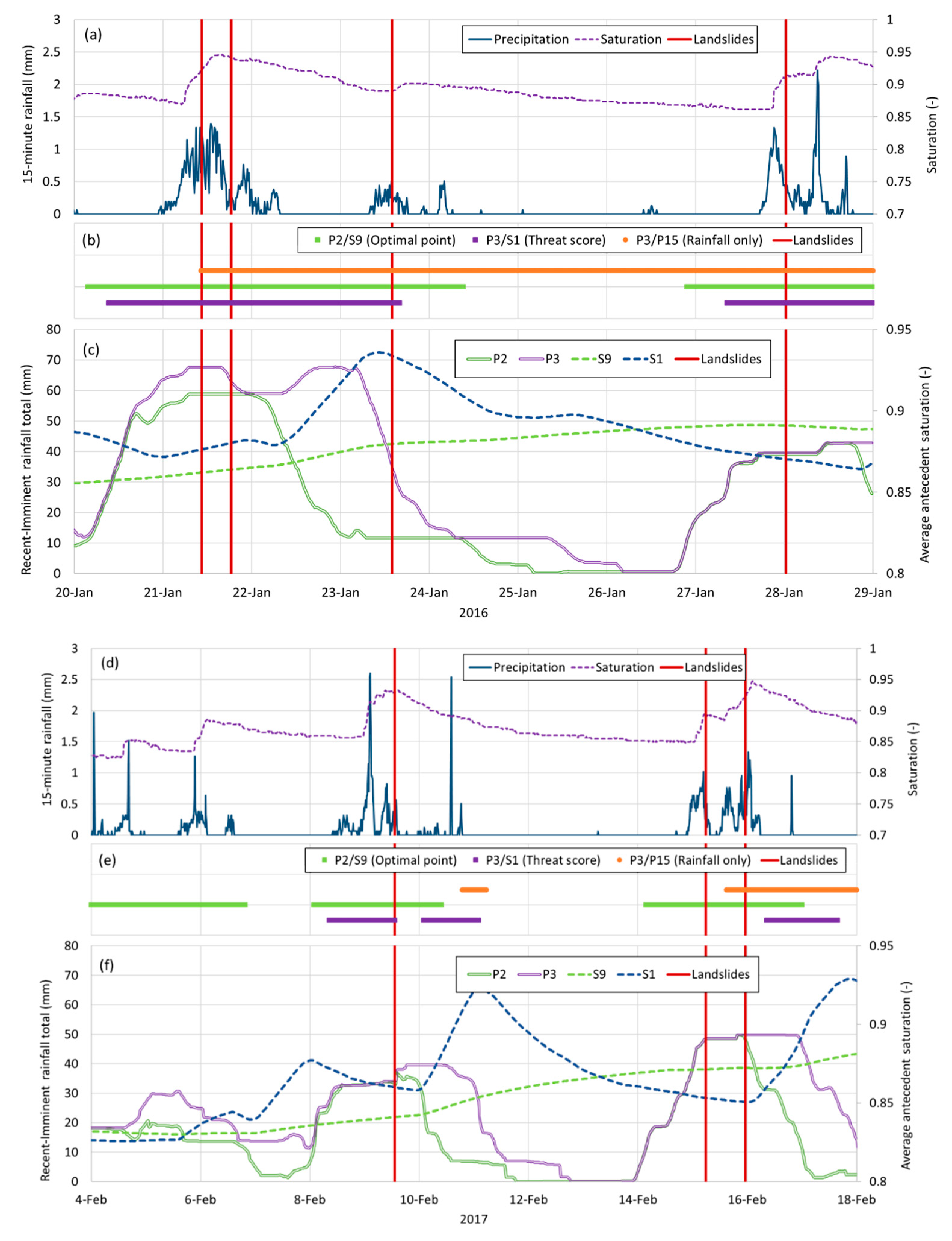
The skill metrics used for optimization have a substantial impact on the TPR and FPR, as well as on the timescales of the threshold spaces (Table 1 and Table 2, Figure 6 and Figure 8), even though the maximum ROC curves share relatively similar shapes and comparable AUC values (Figure 5 and Figure 7). However, it is not immediately clear what these skill metrics mean in terms of utility for landslide forecasting. These somewhat abstract concepts can be illustrated more concretely through an example of how two competing hydro-meteorological thresholds compare to the prior rainfall only threshold [20] for an operational application along the Seattle-Everett railway (Figure 9). A known deficiency of the rainfall only thresholds is the prevalence of sustained false alarms that occur well after the landslide threat has subsided [19,20], which is illustrated for the P3/P15 threshold following landslide events in January and March 2016 as well as in February and March 2017. Rainfall-only thresholds also exhibit frequent false alarms early in the rainy season (October and November) before hillslopes have become sufficiently wet to fail. The hydro-meteorological thresholds optimized with optimal point and threat score (Table 1) both reduce these two systematic varieties of false alarms. The P2/S9 threshold is clearly more averse to failed alarms and therefore misses the fewest landslide events, but also exhibits false alarms during some extended periods of threshold exceedance following most landslide events as well as later in the landslide season (April and May). Conversely, the P3/S1 threshold captures the primary clusters of mid-season landslide events (January through March), but misses the early and late season landslides (December and April, respectively).

The differences between threshold performance can be examined in greater detail by comparing two different landslide-inducing storm sequences. During 21–28 January 2016, particularly heavy precipitation contributed to widespread landsliding across the greater Puget Sound region of Washington, which included multiple landslides along the Seattle-Everett railway (Figure 10a–c). One year later in February 2017, less extensive landsliding occurred along the railway (Figure 10d–f). Time-series of the precipitation and saturation input data, calculated threshold variables and threshold exceedance illustrates how different timescales influence the threshold predictions. The P3/S1 (threat score) threshold is quite precise for the heavy rainfall and widespread landsliding event in January 2016, though the P2/S9 (optimal point) threshold also performs quite well; both correctly illustrate the reduction in landslide hazard during the lull between storms on 25–26 January 2016, whereas the P3/P15 (rainfall only) threshold maintains an extended duration of threshold exceedance. In February 2017, the P3/P15 threshold misses the first two landslides but captures the last one. The more conservative P2/S9 captures all three landslides, but also includes an extended period of false alarms earlier in the month. The more pessimistic P3/S1 captures only the first landslide on 9 February 2017, though it includes a somewhat delayed forecasts of the last two landslides.

These differences in predictive capabilities of the two hydro-meteorological thresholds reflect not only the threshold equations, but also the different timescales of the variables attributed to the cause and trigger components. The S1 variable is a slightly delayed and smoothed signal of the soil moisture dynamics, whereas the S9 variable fluctuates more gradually and reflects a longer-term average of subsurface storage. In contrast, the P2 variable more closely tracks precipitation and the P3 variable retains some memory of prior rainfall events. Although these thresholds are empirical, the different timescales with varying degrees of predictive utility highlights the challenge of distinguishing between cause and trigger from a process-based perspective. Still, comparison of the 15-min input data with the corresponding threshold variables suggests that the shorter timescale P3/S1 threshold more closely tracks observed hydrologic response and therefore may better reflect the underlying processes of rainfall-triggered landslide initiation.

4.2. Dual Alert Systems, Threshold Exceedence and Landslide Occurrence

Although the threat score thresholds include very few false alarms at the expense of some failed alarms, the optimal point thresholds include very few failed alarms at the expense of quite a few false alarms. A threshold with a reasonably good threat score tends to achieve a good precision score as well, but this typically corresponds with lower performance for the true skill statistic and radial distance (e.g., P1/S3 threshold for Portland in Table 2). Similarly, good performance for the true skill statistic and radial distance generally corresponds to a lower threat score and precision (e.g., P2/S9 threshold for Seattle in Table 1). These nuances highlight the role of an informed developer in simultaneously considering data availability, appropriate variables and timescales, threshold equation formats and the intended end-user of the landslide threshold. For example, for both Seattle and Portland, there are minimal differences between the ROC curves and AUC values for the preferred threshold spaces identified using the threat score (Figure 5a and Figure 7a) with their counterparts identified with the optimal point (Figure 5b and Figure 7b). Thus, an informed and observant developer may choose to use the same threshold space for a multi-tiered alert system [14,33], with one threshold that is more pessimistic and one that is more balanced.

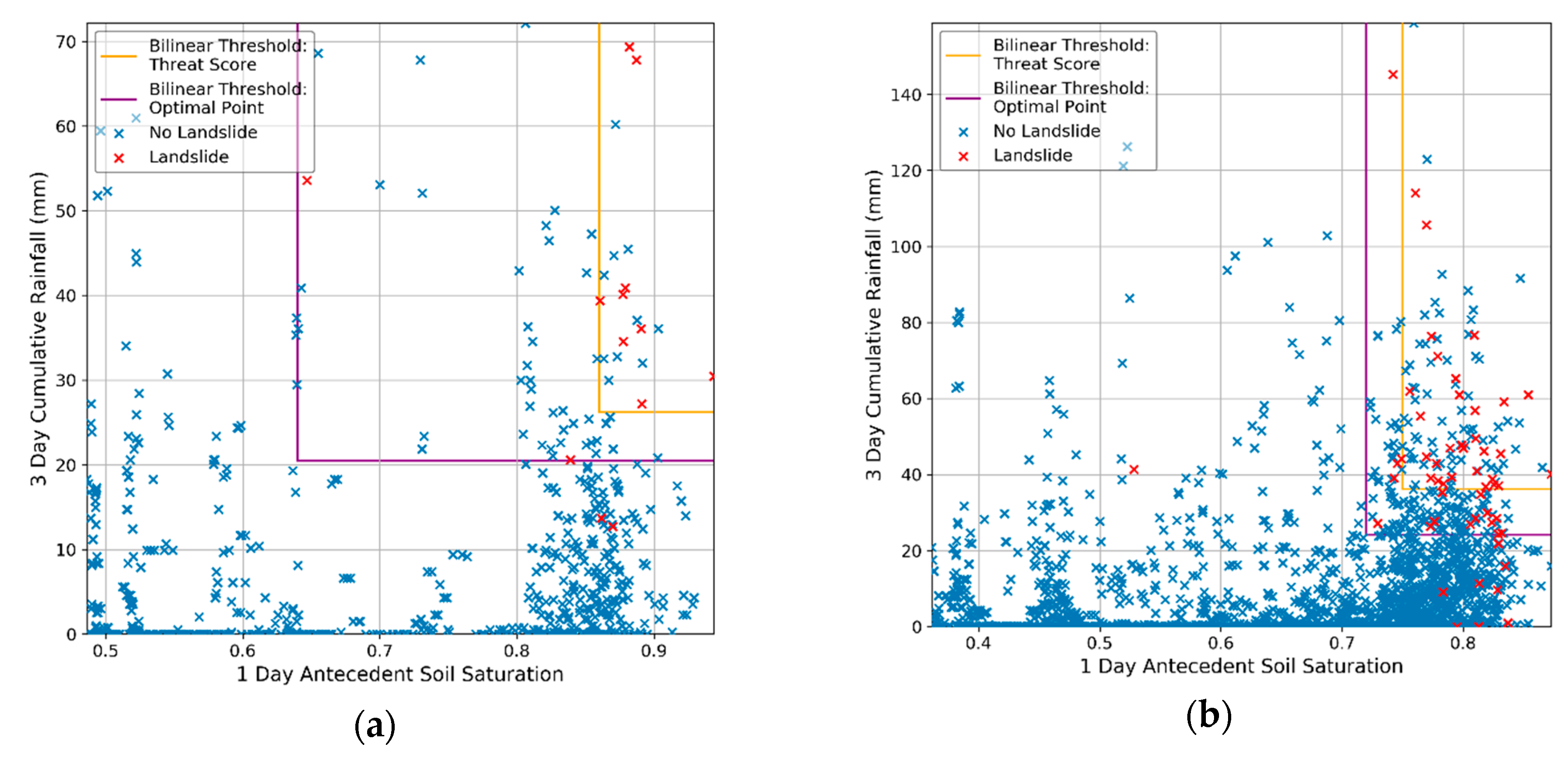
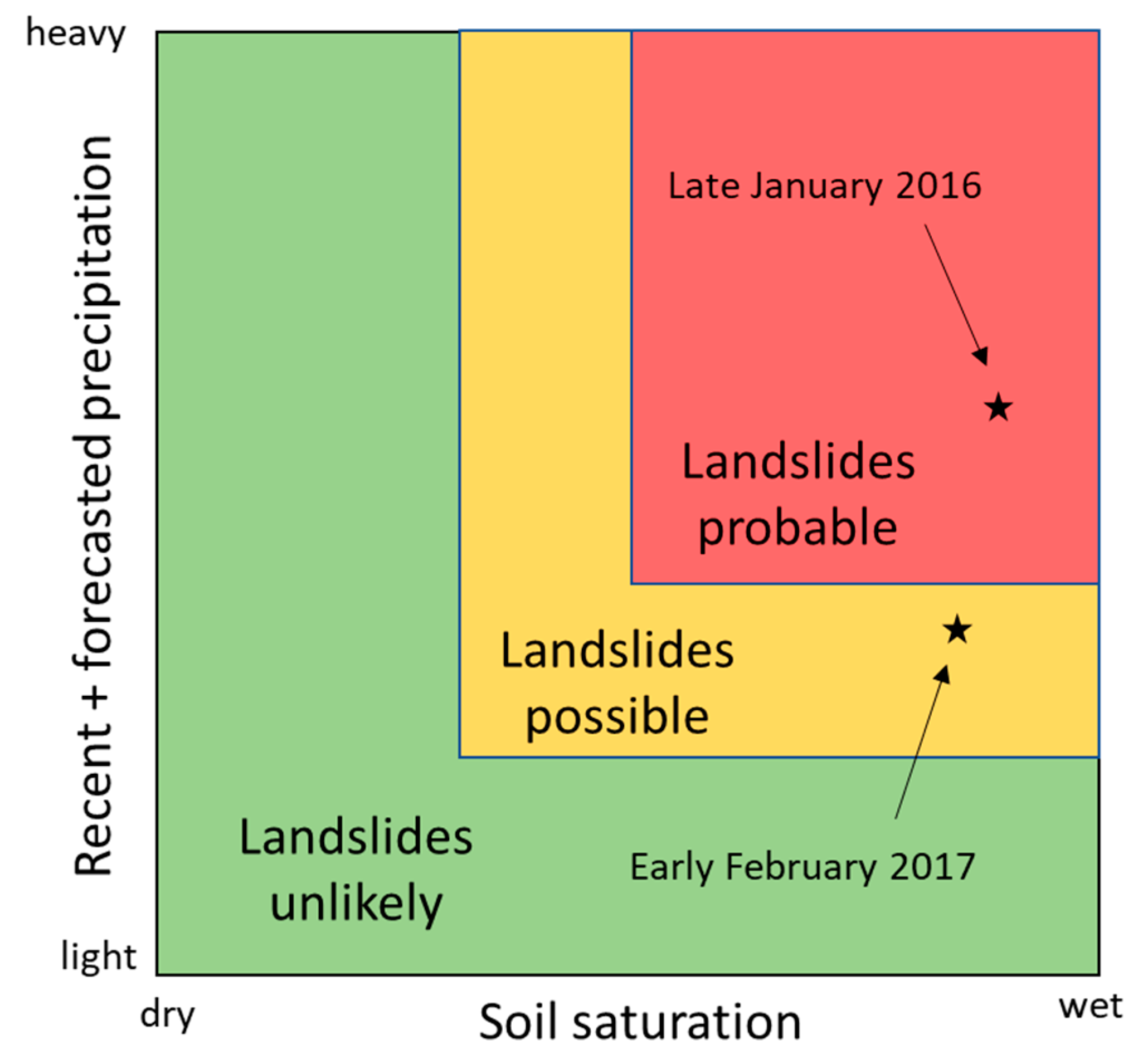
The example shown in Figure 11 includes such dual alert systems for both sites. The threshold spaces are defined by variable timescales identified using the threat score optimization, but include two bilinear thresholds, one optimized with threat score and the other with optimal point. For the Seattle-Everett railway (Figure 11a), this resulted in a P3/S1 space with substantial differences between thresholds optimized for threat score (0.44) and optimal point (0.14). In contrast, a dual alert system for Portland (Figure 11b) also uses the P3/S1 space but includes relatively minor differences between thresholds optimized with threat score (0.53) and optimal point (0.13). Even though the 3-day recent-imminent rainfall and 1-day antecedent saturation timescales for these threshold spaces were optimized with the threat score, there were negligible changes in the radial distances relative to the thresholds optimized with the optimal point (radial distance of 0.13 for both sites) (Table 1 and Table 2). For perspective on the rate of threshold exceedance and utility of the predictions for the Seattle area, landslides occurred on 2.6% of days (Table S1) and the dual thresholds optimized with threat score and optimal point were exceeded 3.4% and 13.2% of days, respectively; in Portland, landslides occurred on 2.5% of days (Table S2) and the dual thresholds were exceeded 3.8% and 12.0% of days. Implementation of this dual alert system could provide an easy-to-interpret tool to communicate when landslides are unlikely, when they are possible and when they are probable (Figure 12).

4.3. Improvements over Established Rainfall-Only Approaches

Although there are no established landslide thresholds for Portland, recently developed rainfall-only thresholds for the Seattle area were optimized using threat score [19,20]. The original Recent-Antecedent (RA) cumulative rainfall threshold [12] achieved a threat score of 0.09 using 3-day recent cumulative rainfall and 15-day antecedent cumulative rainfall as threshold axes. Further objective reanalysis of the RA threshold used the same timescales and threshold space and simple linear equation formulation, but with hourly moving-interval exceedances rather than daily fixed-interval exceedances, which led to a marginally improved threat score 0.11 [20]. Replacing the 15-day antecedent rainfall variable with 15-day antecedent saturation for daily fixed intervals led to a further improved threat score of 0.21 [19]; preliminary exploration of the bilinear threshold with the same threshold variable timescales resulted in a threat score of 0.30 [19]. Here, we use the bilinear threshold formulation and the same daily fixed-interval, but objectively explore alternative timescales for the antecedent soil saturation variable as it relates to landslide initiation. Furthermore, we adopt a recent-imminent rainfall variable with 24 h of accurately predicted rainfall added to prior observed rainfall to reflect the utility of weather forecasts in landslide early warning. Using these methodological developments, we identify optimal threshold variable timescales as 3-day cumulative recent-imminent rainfall and 1-day antecedent saturation, which results in a considerably improved threat score of 0.44 (Table 1). We also explore other threshold optimization metrics for both Seattle and Portland, which identifies shorter optimal timescales of antecedent saturation and leads to minor decreases in threat score, but considerably better optimal point scores and much higher true positive rates (Table 1 and Table 2). The practical utility of these improvements is shown in Figure 9 and Figure 10.

Prior objective testing of rainfall timescales for the Seattle area suggests that 15-day rainfall history is a suitable proxy for antecedent soil saturation prior to a potential landslide-triggering storm [20]. However, we acknowledge that retaining the same 15-day timescale for antecedent saturation [19] lacked any physical meaning or significance. Soil saturation reflects the processes of infiltration, drainage and evapotranspiration that respond dynamically to variable climatic forcing conditions and therefore a shorter timescale might be expected. The differences in timescale of the 15-day antecedent rainfall variable explored previously [12,20] and the considerably shorter durations of the antecedent saturation variables identified objectively in this study reflect the improvements in constraining the hydrological processes relevant to landslide initiation. Although it is tempting to draw inferences from these differences in timescale, it is also important to remember that the hydro-meteorological thresholds explored in this study are empirical and reflect an average of dynamic hydrological processes and the corresponding impact on slope stability. Still, this suggests that physics-based modeling of hydrologic response for shallow landslide hazard assessment in these regions could focus on 3-day event-based simulations with appropriate initial conditions.

4.4. Versatility of the Hydro-Meterological Threshold Approach

In many regions where rainfall-induced shallow landsliding is a concern, the antecedent saturation is the predisposing factor whereas the actual landslide initiation is associated with hydrologic response to the recent and incoming rainstorm. Our approach for hydro-meteorological threshold identification and optimization is guided by this cause-trigger concept [18]. Our proposed method is semi-automated and not completely objective, but this is by design. We remain convinced that selection of the appropriate threshold variables and timescale as well as the preferred optimization metric should be an informed and conscious choice by the threshold developer. This subjective component not only prevents unreasonable threshold spaces from being selected automatically, but it also allows some degree of discretion regarding the balance between the reliability of certain data inputs and rainfall forecasts, the accuracy of competing threshold formulations and ratio of failed to false alarms.

Here, we explore different threshold timescales and formats by building off prior usage of soil saturation for the antecedent hydrologic cause component and rainfall as the recent triggering variable [19]. However, our proposed protocol is not strictly limited to the dual rainfall-saturation variables. We do advocate using rainfall to represent the meteorological triggering factor, since weather forecasts can be leveraged to incorporate imminent rainfall conditions into greater lead-times, but a variety of subsurface monitoring data could represent the predisposing hydrological factors. Saturation is an intuitive variable and can be derived using a range of measurement techniques, including point measurements with reliable low-cost VWC sensors [23,24,25] or satellite remote sensing estimates of soil moisture [34]. We acknowledge that variably saturated pore-water pressures are more closely linked to the process of landslide initiation [14,15,16,17,18], but it is also a more expensive and difficult variable to measure continuously [22,24,25].

For our datasets, landslide events typically clustered in the upper right corner of the various threshold spaces (Figure 4, Figure 6, Figure 8 and Figure 11), which further supports the use of bilinear thresholds rather than the simple linear thresholds used previously [19,20]. However, one could also employ more complex exponential or polynomial functions, such as those used for intensity-duration thresholds [11]. We found that prior improvements from updating the threshold format from simple linear to bilinear [19] were similar when incorporating accurate 24 h forecasts into the 3-day cumulative rainfall variable (Figure 4a). However, this may not be universally true for all geographic settings or landslide databases, or even for different threshold variables. If landslide events do not plot in a cluster in the corner of a selected threshold space, it is possible that other threshold formats may be more appropriate. Furthermore, comparison of the thresholds optimized with threat score (Figure 5a, Figure 6a, Figure 7a and Figure 8a) with those optimized using the optimal point (Figure 5b, Figure 6b, Figure 7b and Figure 8b) illustrates how the metric influences the timescales and equations for optimal thresholds and their practical utility for landslide early warning systems (Figure 9 and Figure 10).

4.5. Avenues for Further Investigation and Improvements

For the Seattle area, a few off-season landslides occurred when antecedent saturation values were relatively low (Figure 6), but using the present saturation instead of antecedent saturation to represent the cause variable might have produced more accurate thresholds. This issue may reflect the inherent heterogeneity within a given geographic area, where the onset of strong seasonal dynamics varies between neighboring hillslopes depending on vegetation, slope aspect, soil properties and even human activities. For example, in a similar location along the Seattle-Everett railway, observations indicate that soil moisture and pore pressures respond differently to early versus mid-season storms [23]. Similarly, observations from additional monitoring sites suggest that recent landslides wet-up earlier in the winter rainy season and drain slower in the dry season relative to neighboring stable hillslopes [35]. Thus, they are predisposed to reactivation during larger early or late season storms that do not initiate new failures on adjacent hillslopes. This presents an issue for hydrologic threshold development, which could be addressed through a distributed assessment of soil moisture that reflects relevant types of variability within the area of interest.

Comparison of our two cases from the Seattle-Everett railway and the City of Portland are complicated by differences in the instrumentation configuration and duration of the datasets, as well as other differences between the two inventories (e.g., only railway blocking events compared to all landslides within a city limit). The Portland dataset includes several days with numerous landslides (Table S2), which are obviously very important from an early warning perspective. The inventory of landslides blocking the Seattle-Everett railway includes only a few multiple landslide days (Table S1) and most notably the period in late January 2016 (Figure 10a–c) when heavy rainfall across the Puget Sound area produced widespread landsliding. The Portland site includes a combination of deeper and shallower probes installed at one location (Figure 3), whereas the site along the Seattle-Everett railway includes a hillslope transect of probes all installed at or near the expected failure depth (Figure 2). The different instrument configurations between the two sites [24,25] likely has an intertwined impact on both the threshold formulations and their performance, but we were not able to address this level of complexity. Instrument arrangement and placement is often constrained by site access, vegetation, soil depth and budgetary considerations, which complicates the process of designing optimal instrument networks for informing hydro-meteorological thresholds. Furthermore, the longer duration of monitoring and greater number of landslides for Portland result in a smoother ROC curve and decrease the impact of individual landslide days. Further testing of our approach with more recent landslides and monitoring data from these sites or other long-term datasets with different instrument configurations could help inform improved network design for future monitoring sites.

The accuracy of quantitative precipitation forecasts can influence threshold predictions in advance of an incoming storm [14]. However, the uncertainty in rainfall forecasts may vary from storm to storm and from location to location, which was not the focus of this study. Instead we rely on the assumption that measured rainfall is equivalent to the 24 h forecast, which follows the precedent of our operational implementation of existing USGS rainfall-only thresholds for Seattle, namely we assume that 24 h rainfall forecasts from the U.S. National Weather Service (NWS) [36] are sufficiently accurate to incorporate directly into the recent-rainfall threshold variable [27]. In contrast, incorporating longer-term quantitative precipitation forecasts (e.g., 72 h) into any type of landslide threshold should weigh the trade-off between the likely impact of forecast uncertainty on threshold accuracy against the possible benefits of greater lead-times for warnings. Such an assessment is complicated by considerable variation in forecast accuracy depending on the study area, type of storm, and timescale.

Theoretically, timescales of mixed-number daily values (e.g., 2.5 days) can be selected for threshold input variables to further improve our thresholds for Portland and the Seattle area, but we observed relatively incremental changes in threshold performance metrics with one-day (24 h) changes in both threshold variables for these two sites. Therefore, we opted to consider daily intervals for our threshold timescales, since this integrates well with NWS quantitative precipitation forecasts and is likely more intuitive for end-users to interpret than fractional days of cumulative rainfall or antecedent saturation. On the other hand, relatively small changes in the ROC curves can still impact the AUC and other metrics due to the high number of non-landslide days (i.e., negative events). Depending on the availability of detailed forecasting and precise landslide timing information and the intended target audience for a landslide warning system, threshold developers using our method could explore timescales that include fractions of days (or hours) to identify a more objectively optimized threshold with slightly better predictive capabilities at the expense of less intuitive inputs. Again, the flexibility of our semi-automated approach would allow threshold developers to make their own judgments regarding these types of trade-offs.

5. Conclusions

Following the cause-trigger concept of hydro-meteorological thresholds for shallow landsliding and prior work to explore specific rainfall-saturation thresholds using real-time monitoring, we propose a general method to identify and optimize such thresholds that can inform warning systems by leveraging monitoring data and rainfall forecasts. We explored alternative durations of accumulated recent plus 24 h imminent rainfall as the meteorological triggering threshold variable, which we use in combination with the antecedent soil wetness conditions as the hydrologic cause variable. Using examples from field monitoring sites and landslide inventories in the Seattle area, Washington and City of Portland, Oregon, we illustrate how the method could be implemented for defining thresholds with different priorities. The results include development of new landslide thresholds that can be used for situational awareness in Portland and further improvements to the rainfall-only threshold already used by emergency planners and citizens in the Seattle area. These sets of thresholds are distinct from one another, reflecting in part the differences in hydrological conditions that favor the predisposing and triggering factors for landsliding in these two distinct areas of the Pacific Northwest, USA. Our approach for developing new thresholds could be useful over a wide range of settings where the cause of shallow landsliding can be attributed to the antecedent wetness and the triggering is associated with a storm event, particularly when rainfall forecasts are sufficiently accurate. These improvements in landslide early warning from hydro-meteorological thresholds can ultimately help reduce losses resulting from landslides.

References

1. Guzzetti, F.; Peruccacci, S.; Rossi, M.; Stark, C.P. The rainfall intensity-duration control of shallow landslides and debris flows: An update. Landslides 2008, 5, 3–17. [Google Scholar] [CrossRef]
2. Baum, R.L.; Godt, J.W. Early warning of rainfall-induced shallow landslides and debris flows in the USA. Landslides 2010, 7, 259–272. [Google Scholar] [CrossRef]
3. Segoni, S.; Piciullo, L.; Gariano, S.L. A review of the recent literature on rainfall thresholds for landslide occurrence. Landslides 2018, 15, 1483–1501. [Google Scholar] [CrossRef]
4. Staley, D.M.; Kean, J.W.; Cannon, S.H.; Schmidt, K.M.; Laber, J.L. Objective definition of rainfall intensity-duration thresholds for the initiation of post-fire debris flows in southern California. Landslides 2013, 10, 547–562. [Google Scholar] [CrossRef]
5. Jakob, M.; Owen, T.; Simpson, T. A regional real-time debris-flow warning system for the District of North Vancouver, Canada. Landslides 2012, 9, 165–178. [Google Scholar] [CrossRef]
6. Caine, N. The rainfall intensity-duration control of shallow landslides and debris flows. Geogr. Ann. Ser. A Phys. Geogr. 1980, 62, 23–27. [Google Scholar] [CrossRef]
7. Leonarduzzi, E.; Molnar, P.; McArdell, B.W. Predictive performance of rainfall thresholds for shallow landslides in Switzerland from gridded daily data. Water Resour. Res. 2017, 53, 6612–6625. [Google Scholar] [CrossRef]
8. Rosi, A.; Peternel, T.; Jemec-Auflič, M.; Komac, M.; Segoni, S.; Casagli, N. Rainfall thresholds for rainfall-induced landslides in Slovenia. Landslides 2016, 13, 1571–1577. [Google Scholar] [CrossRef]
9. Glade, T.; Crozier, M.J.; Smith, P. Applying Probability Determination to Refine Landslide-triggering Rainfall Thresholds Using an Empirical “Antecedent Daily Rainfall Model”. Pure Appl. Geophys. 2000, 157, 1059–1079. [Google Scholar] [CrossRef]
10. Crozier, M.J. Prediction of rainfall-triggered landslides: A test of the antecedent water status model. Earth Surf. Process. Landf. 1999, 24, 825–833. [Google Scholar] [CrossRef]
11. Godt, J.W.; Baum, R.L.; Chleborad, A.F. Rainfall characteristics for shallow landsliding in Seattle, Washington, USA. Earth Surf. Process. Landf. 2006, 31, 97–110. [Google Scholar] [CrossRef] [Green Version]
12. Chleborad, A.F.; Baum, R.L.; Godt, J.W.; Powers, P.S. A prototype system for forecasting landslides in the Seattle, Washington, area. In Landslides and Engineering Geology of the Seattle, Washington, Area; Baum, R.L., Godt, J.W., Highland, L., Eds.; Geological Society of America: Boulder, CO, USA, 2008; pp. 103–120. [Google Scholar]
13. Segoni, S.; Rosi, A.; Lagomarsino, D.; Fanti, R.; Casagli, N. Brief communication: Using averaged soil moisture estimates to improve the performances of a regional-scale landslide early warning system. Nat. Hazards Earth Syst. Sci. 2018, 18, 807–812. [Google Scholar] [CrossRef] [Green Version]
14. Thomas, M.A.; Mirus, B.B.; Collins, B.D. A physics-based approach to identify thresholds for rainfall-induced shallow landsliding. Geophys. Res. Lett. 2018, GRL58002. [Google Scholar] [CrossRef]
15. Salvatici, T.; Tofani, V.; Rossi, G.; D’Ambrosio, M.; Tacconi Stefanelli, C.; Masi, E.B.; Rosi, A.; Pazzi, V.; Vannocci, P.; Petrolo, M.; et al. Application of a physically based model to forecast shallow landslides at a regional scale. Nat. Hazards Earth Syst. Sci. 2018, 18, 1919–1935. [Google Scholar] [CrossRef]
16. Fusco, F.; De Vita, P.; Baum, R.L.; Mirus, B.B.; Allocca, V.; Tufano, R.; Calcaterra, D. Hydrological monitoring and modeling approaches for assessing timing of shallow landslide in the volcanic area of the Phlegrean Fields (southern Italy). Landslides 2018. in review. [Google Scholar]
17. Napolitano, E.; Fusco, F.; Baum, R.L.; Godt, J.W.; De Vita, P. Effect of antecedent-hydrological conditions on rainfall triggering of debris flows in ash-fall pyroclastic mantled slopes of Campania (southern Italy). Landslides 2016, 13, 967–983. [Google Scholar] [CrossRef]
18. Bogaard, T.; Greco, R. Invited perspectives: A hydrological look to precipitation intensity duration thresholds for landslide initiation: Proposing hydro-meteorological thresholds. Nat. Hazards Earth Syst. Sci. 2018, 18, 31–39. [Google Scholar] [CrossRef]
19. Mirus, B.B.; Becker, R.; Baum, R.L.; Smith, J.B. Integrating real-time subsurface hydrologic monitoring with empirical rainfall thresholds to improve landslide early warning. Landslides 2018, 15, 1909–1919. [Google Scholar] [CrossRef]
20. Scheevel, C.R.; Baum, R.L.; Mirus, B.B.; Smith, J.B. Precipitation Thresholds for Landslide Occurrence Near Seattle, Mukilteo, and Everett, Washington; GSGS: Reston, VA, USA, 2017. [Google Scholar]
21. Ciavoletta, M.; Bogaard, T.; Gargano, R.; Greco, R. Is there predictive power in hydrological catchment information for regional landslide hazard assessment? Procedia Earth Planet. Sci. 2016, 16, 195–203. [Google Scholar] [CrossRef]
22. Torres, R.; Dietrich, W.E.; Montgomery, D.R.; Anderson, S.P.; Loague, K. Unsaturated zone processes and the hydrological response of a steep unchanneled catchment. Water Resour. Res. 1998, 34, 1865–1879. [Google Scholar] [CrossRef]
23. Baum, R.L.; McKenna, J.P.; Godt, J.W.; Harp, E.L.; McMullen, S.R. Hydrologic Monitoring of Landslide-Prone Coastal Bluffs near Edmonds and Everett, Washington, 2001–2004; GSGS: Reston, VA, USA, 2005. Available online: https://pubs.usgs.gov/of/2005/1063/ (accessed on 27 January 2005).
24. Smith, J.B.; Baum, R.L.; Mirus, B.B.; Michel, A.; Stark, B. Results of Hydrologic Monitoring on Landslide Prone Coastal Bluffs near Mukilteo, Washington; GSGS: Reston, VA, USA, 2017. [Google Scholar]
25. Smith, J.B.; Godt, J.W.; Baum, R.L.; Coe, J.A.; Ellis, W.L.; Jones, E.S.; Burns, S.F. Results of Hydrologic Monitoring of a Landslide-Prone Hillslope in Portland’s West Hills, Oregon, 2006–2017; GSGS: Reston, VA, USA, 2017. [Google Scholar]
26. Statewide Landslide Information Database for Oregon (SLIDO), Release 3.2. Available online: https://www.oregongeology.org/slido/ (accessed on 26 July 2018).
27. Seattle Area, Washington. Available online: https://www.usgs.gov/natural-hazards/landslide-hazards/science/seattle-area-washington?qt-science_center_objects=0#qt-science_center_objects (accessed on 7 September 2018).
28. Portland, Oregon. Available online: https://www.usgs.gov/natural-hazards/landslide-hazards/science/portland-oregon?qt-science_center_objects=0#qt-science_center_objects (accessed on 7 September 2018).
29. Mirus, B.B.; Smith, J.B.; Stark, B.; Lewis, Y.; Michel, A.R.; Baum, R.L. Assessing Landslide Potential on Coastal Bluffs near Mukilteo, Washington—Geologic Site Characterization for Hydrologic Monitoring; GSGS: Reston, VA, USA, 2016. [Google Scholar]
30. Swets, J.A. Measuring the accuracy of diagnostic systems. Science 1988, 240, 1285–1293. [Google Scholar] [CrossRef] [PubMed]
31. Fawcett, T. An introduction to ROC analysis. Pattern Recognit. Lett. 2006, 27, 861–874. [Google Scholar] [CrossRef]
32. Postance, B.; Hillier, J.; Dijkstra, T.; Dixon, N. Comparing threshold definition techniques for rainfall-induced landslides: A national assessment using radar rainfall. Earth Surf. Process. Landf. 2018, 43, 553–560. [Google Scholar] [CrossRef]
33. Piciullo, L.; Gariano, S.L.; Melillo, M.; Brunetti, M.W.; Peruccacci, S.; Guzetti, F.; Calvello, M. Definition and performance of a threshold-based regional early warning model for rainfall-induced landslides. Landslides 2017, 14, 995–1008. [Google Scholar] [CrossRef]
34. Brocca, L.; Ciabatta, L.; Moramarco, T.; Ponziani, F.; Berni, N.; Wagner, W. Use of Satellite Soil Moisture Products for the Operational Mitigation of Landslides Risk in Central Italy. In Satellite Soil Moisture Retrievals: Techniques & Applications; Petropoulos, G.P., Srivastava, P., Kerr, Y.H., Eds.; Elsevier: Amsterdam, The Netherlands, 2016; pp. 231–247. [Google Scholar] [CrossRef]
35. Mirus, B.B.; Smith, J.B.; Baum, R.L. Hydrologic Impacts of Landslide Disturbances: Implications for Remobilization and Hazard Persistence. Water Resour. Res. 2017, WRCR22885. [Google Scholar] [CrossRef]
36. National Weather Service. Available online: https://weather.gov (accessed on 7 September 2018).
Figure 1. Schematic flow-chart of iterative, semi-automated process to identify appropriate threshold space, defined by input variables and timescales and optimize preferred threshold equation using receiver operating characteristics (ROC) analysis. Blue boxes and arrows indicate user input, red boxes and arrows indicate automated calculations, green boxes and arrows indicate user decisions.
Water 10 01274 g001
Figure 2. (a) Map of the monitoring location along the Seattle-Everett railway in Mukilteo, Washington, USA. Inset lidar image shows hillslope transect location (in blue); (b) Hillslope transect with five VWC instrument locations and depths and aerial image of the field site. Adapted from Mirus et al., 2016 [29].
Water 10 01274 g002
Figure 3. (a) Map of the Portland Hills monitoring site in Portland, Oregon, USA, on shaded hillslope image with topographic contours; (b) Detail showing various instrument locations on aerial image. Reproduced from Smith et al., 2017 [25].
Water 10 01274 g003
Figure 4. (a) Hydro-meteorological threshold space defined by 15-day antecedent saturation vs. 3-day recent-imminent rainfall (2-day recent, 1-day forecasted) totals for the Seattle-Everett railway, with comparison of simple linear (purple) and bilinear (yellow) threshold formats; (b) Example ROC plots showing the true positive rate (TPR) and false positive rate (FPR) with colored stars for the simple linear (yellow) and bi-linear (purple) thresholds. Plot also illustrates a hypothetical threshold development and the concept of identifying the maximum ROC curve based on clusters of points from possible thresholds tested and shows the utility of AUC as an optimization metric; dashed black line represents a random guess model (AUC = 0.5), blue (AUC = 0.67), green (AUC = 0.75) and orange lines (AUC = 0.95) represent successive improvements in threshold formulation and predictive accuracy.
Water 10 01274 g004
Figure 5. Seattle area ROC curves showing the performance of different threshold formats optimized with: (a) threat score; (b) optimal point statistic. Optimal thresholds for each ROC curve are shown as the solid dots. Recent rainfall and Saturation for N days shown as PN and SN, respectively.
Water 10 01274 g005
Figure 6. Seattle area hydro-meteorological threshold plots showing competing thresholds optimized with: (a) threat score; (b) optimal point statistic. Predicted landslide(s) are TP; false alarms are FP; no landslides are TN; missed landslide(s) are FN.
Water 10 01274 g006
Figure 7. City of Portland ROC curves showing the performance of different threshold formats optimized with: (a) threat score; (b) optimal point statistic. Optimal thresholds for each curve are shown as the solid dots. Recent rainfall and saturation for N days shown as PN and SN, respectively.
Water 10 01274 g007
Figure 8. City of Portland hydro-meteorological threshold plots showing competing thresholds optimized with: (a) threat score; (b) optimal point statistic. Predicted landslide(s) are TP; false alarms are FP; no landslides are TN; missed landslide(s) are FN.
Water 10 01274 g008
Figure 9. Time-series of landslide occurrence and threshold exceedance during two sequential landslide seasons (2015–2016 and 2016–2017) for the Seattle-Everett railway, with competing thresholds P2/S9 (optimal point) and P3/S1 (threat score) optimized in this study (Table 1) and the previously established P3/P15 (rainfall only), which was also optimized with threat score [20].
Water 10 01274 g009
Figure 10. Time-series for the greater Seattle area illustrating the observed landslide occurrences along the railway relative to 15-min resolution, during the widespread landsliding event in January 2016: (a) measured precipitation and saturation [24]; (b) exceedance of competing landslide thresholds optimized with the optimal point (P2/S9) and threat score (P3/S1) for this study (Table 1) and the established rainfall only threshold [20] optimized with threat score (P3/P15); and (c) hydro-meteorological threshold variables with different timescales. Similar time-series during a less widespread landsliding sequence in February 2017 are shown in (df).
Water 10 01274 g010
Figure 11. Dual hydro-meteorological threshold plots optimized with threat score and optimal point statistics for (a) Seattle-Everett railway and (b) City of Portland.
Water 10 01274 g011
Figure 12. Qualitative example of an operational implementation of the dual hydro-meteorological threshold plots, showing a general audience when landslides are unlikely, possible and probable. Whereas the late January 2016 events in Seattle would have plotted in the highest hazard zone, the early February 2017 events would likely have plotted in the moderate hazard zone (see Figure 10).
Water 10 01274 g012