Article

Evaluating the Erosion Process from a Single-Stripe Laser-Scanned Topography: A Laboratory Case Study

Department of Soil and Water Conservation, National Chung Hsing University, Taichung 402, Taiwan
*
Author to whom correspondence should be addressed.
Water 2018, 10(7), 956; https://doi.org/10.3390/w10070956
Submission received: 30 May 2018 / Revised: 6 July 2018 / Accepted: 17 July 2018 / Published: 19 July 2018
(This article belongs to the Special Issue Modeling and Practice of Erosion and Sediment Transport under Change)

Abstract

:
Topographies during the erosion process obtained from the single-stripe laser-scanning method may provide an accurate, but affordable, soil loss estimation based on high-precision digital elevation model (DEM) data. In this study, we used laboratory erosion experiments with a sloping flume, a rainfall simulator, and a stripe laser apparatus to evaluate topographic changes of soil surface and the erosion process. In the experiments, six slope gradients of the flume (5° to 30° with an increment of 5°) were used and the rainfall simulator generated a 30-min rainfall with the kinetic energy equivalent to 80 mm/h on average. The laser-scanned topography and sediment yield were collected every 5 min in each test. The difference between the DEMs from laser scans of different time steps was used to obtain the eroded soil volumes and the corresponding estimates of soil loss in mass. The results suggest that the collected sediment yield and eroded soil volume increased with rainfall duration and slope, and quantified equations are proposed for soil loss prediction using rainfall duration and slope. This study shows the applicability of the stripe laser-scanning method in soil loss prediction and erosion evaluation in a laboratory case study.

1. Introduction

Rill and interrill erosion are the major intermediate processes between sheet and gully erosion on hillslopes. As the main source that causes soil loss on sloping croplands and rangelands, rill erosion provides 76% of the total sediment load eroded from hillslopes [1]. In an eroding rill, the flow concentrates and results in hydrodynamic characteristics with an increasing scouring power, and thus leads to a significant increase in soil erosion [2]. Meanwhile, the development of a rill network results in a threefold soil loss increment [3], and the eroding rills become the primary channels for sediment transport. It is reported that more than 80% of the eroded soil is transported through rills [4,5]. Therefore, rill development not only has its significance in erosion process evaluation, but also shows an implication for drainage network evolution on hillslopes.
The evolution of rill networks and rill morphology progresses in time and space [6]. Rill networks develop with varying complexity, leading to flow concentration and increasing runoff connectivity along the networks [7]. Variations in rill morphology interact with soil erosion processes, including detachment, transport, and deposition, which are dependent on the hydrodynamic features and transport capacity of the flow in rills [8]. Complex feedback exists in rill erosion mechanics, since the flow erodes soil and changes the rill bed surface, which in turn alters the hydrodynamic features and transport capacity of the flow [9]. In general, a rill flow with a higher velocity and deeper depth provides a larger transport capacity for carrying sediments, leading to more variations in rill morphology.
In erosion process evaluation, the evolution of a rill network and rill morphology has been a focus to develop and improve process-based erosion models and prediction [5,10]. While the topography caused by rill erosion is often complicated and irregular, a rill-by-rill survey is difficult and even impractical in the field [1], and field-scale experiments are limited to qualitative or semi-quantitative descriptions [11]. Therefore, quantification of the rill erosion process has become an essential but challenging issue. At the laboratory scale, rainfall simulators are widely applied in research on infiltration and soil erosion processes for mimicking the process and characteristics of natural rainfall [12]. In order to replicate rill erosion processes, rainfall simulation has its advantages in producing rainfall events at an arbitrary intensity and duration on demand; thereby, the erratic and unpredictable variability of natural rains can be eliminated [12]. Most of the previous studies on erosion process evaluation have developed quantification methods for rill erosion and rill network development using rainfall simulators to produce rainfall events on laboratory flumes or field plots.
Among the rill erosion research, many types of rill erosion quantification methods have been applied, such as collecting sediment outflow at the flume end [12], a volumetric or volume replacement method [2,13,14], manual measurements of rills using photo images [1,15], photogrammetry methods [16,17,18,19], a terrestrial laser scanner (TLS) [5,20,21,22,23], an airborne laser scanner (ALS) [24,25], and other remote-sensing technologies. In [12], laboratory erosion experiments were carried out in a two-dimensional tilting flume with a pre-forming rill before the rainfall application on the soil surface; then, rill and interrill erosion were assessed by flow measurements taken from the two outlets, corresponding to the rill and interrill area, at the end of the flume.
The volumetric method measures and calculates the cross-sectional areas along the eroded rills and estimates the eroded soil volume [14]. The volume replacement method uses other materials, such as soil, tiny foam particles, rice grains, and water, to refill rills and measure the rill volume by the filling materials to estimate the erosion volume [2,13]. Specifically, water is used to refill the eroded rills in order to minimize the measurement errors due to the difficulty of rill identification in the cases of not-well-confined rills and various rill sizes [2]. However, sealing of the soil surface, which prevents infiltration and further erosion, is the key factor for precise measurements of the rill volume and may become the major source of error in practice. Manual measurements of rills using photo images are applied in laboratory studies [1,15] for obtaining each rill’s width, depth, and location coordinates along with rainfall duration from photographs taken of the soil surface in 1- or 2-min intervals throughout each rainfall event. The manual measurement method is usually time- and force-consuming and can be dependent on subjective judgement of rill boundaries.
Methods of photogrammetry are applied to assess soil erosion in laboratory-scale experiments [16,17,18,19]. Estimation of soil erosion using small-scale laboratory erosion experiments was carried out by the method of structure-from-motion (SfM) photogrammetry [16]. Digital elevation models (DEMs) of a 0.5 m2 soil box were built by the photogrammetric SfM technique, and the computed sediment yield was obtained by the DEM of difference (DoD) technique [16]. They proposed that the choice of DoD threshold was a key point that affects the computed sediment yield; the results show that the computed sediment yield was 13% greater than the measured sediment yield [16]. Rill development and soil erosion was studied using a gravity-type rainfall simulator, a tilting box filled with sand and soil material, and photogrammetric equipment [17]. In this research, stereo imagery was taken from two positions to generate DEMs of the soil surface, which were used to analyze soil surface and rill network changes between the time steps of rainfall events. The results suggest that rill density and energy expenditure decreased with time [17]. The application of a close-range photogrammetry method for soil erosion assessment and a comparison between photogrammetry and laser-scanner technology in producing DEMs and soil surface elevation differences are shown in previous studies [18,19]. While both of the studies were carried out using laboratory flumes, they suggest the potential of the photogrammetry method in field applications provided the limitations of the technique are considered [18,19].
The application of the TLS technique in soil erosion and rill development evaluation can be found in laboratory, plot, and field studies [5,20,21,22,23]. The study of the morphological characteristics of rill evolution was performed using laboratory soil pan rainfall simulations [5] and the TLS technique following [20]. They proposed quantitative descriptions of a rill network using the fractal dimension, which was analyzed from the TLS data and the resulting DEMs. To evaluate soil erosion at the plot scale, uses three types of TLS are used to measure the topography before and after the manual removal of some soil volume (to imitate soil erosion) of a field plot about 30 m × 30 m in size with a 20° slope [21]. The results show that soil erosion measured with TLS varies considerably when different data processing software is used, and the laser-scanning technique is applicable in measuring soil erosion at the plot scale when adequate calibration and spatial resolution are performed [21]. In field investigations of soil erosion using TLS [20,22,23], rill morphology and soil loss evaluation at the Masse experimental station in Italy were studied [20]. The triangulated irregular network model was used to quantify the eroded volume and rill morphological characteristics; corresponding manual measurements were also carried out using a profilometer [20]. A basin-scale assessment of riverbank erosion in Northern Italy was monitored, and the eroded and deposited volume in the surveyed area were measured using TLS [22]. The effects of TLS to analyze the intensity of soil erosion in a mountainous forest area with sufficient measurement stations are shown [23]. As the results indicate, choices of the coordinate system for the object or the scanner significantly influence the analysis of erosion phenomena when applying TLS in forested areas [23].
The technique of ALS has also been applied in field studies to assess riverbank erosion [24] and characterize land degradation processes [25]. ALS was used to obtain detailed topographic data for characterizing sediment and phosphorous contributions from riverbank erosion of the Blue Earth River in southern Minnesota, USA [24]. Since the source of error and the uniformity within and between the scans were difficult to determine, no elevation or planimetric corrections of the laser data were made in the study. Nevertheless, the soil loss estimates obtained by ALS locate in the range of the reported literature values for the same study site. The land degradation processes, including soil erosion, channel incision, and collapse sinkholes development in the Dead Sea region, are quantified using ALS [25]. The results demonstrate the ability of ALS to detect sub-metric geomorphic features, such as gullies, headcuts, and embryonic sinkholes, which can occur in land degradation processes [25]. Other remote-sensing technologies, such as an Unmanned Aerial Vehicle (UAV), Time-of-Flight (ToF) cameras (or range cameras), and airborne and terrestrial Light Detection and Ranging (LiDAR) [20], have been applied to investigate topographic evolution in the field, and have their potential and applicability in soil erosion and land degradation process evaluation, but are usually expensive in cost and/or require delicate operating and data-processing skills.
In this study, we took advantage of the high resolution provided by the laser-scanning technique but used a more affordable stripe laser apparatus, compared to a three-dimensional (3D) laser scanner, to construct the erosion topography for erosion process evaluation. At the laboratory scale, erosion processes on slopes were reproduced in an adjustable slope flume with a rainfall simulator, and a series of laser-scanned topographies during the erosion process was obtained by the stripe laser apparatus for evaluating the rill development, erosion progress, and the eroded soil volume. The effects of rainfall duration and slope on the eroded soil volume and sediment yield were quantified using a multiple regression analysis. By comparing the eroded volume with the outflow sediments collected from the flume outlet, a quantified relation was proposed between the eroded soil volume and the sediment yield at the outlet of the sloping flume. The results of this study present a quantified evaluation of the influences of rainfall duration and slope on the erosion process and a prediction of the sediment yield using single-stripe laser-scanned topography in a laboratory flume case study.

2. Materials and Methods

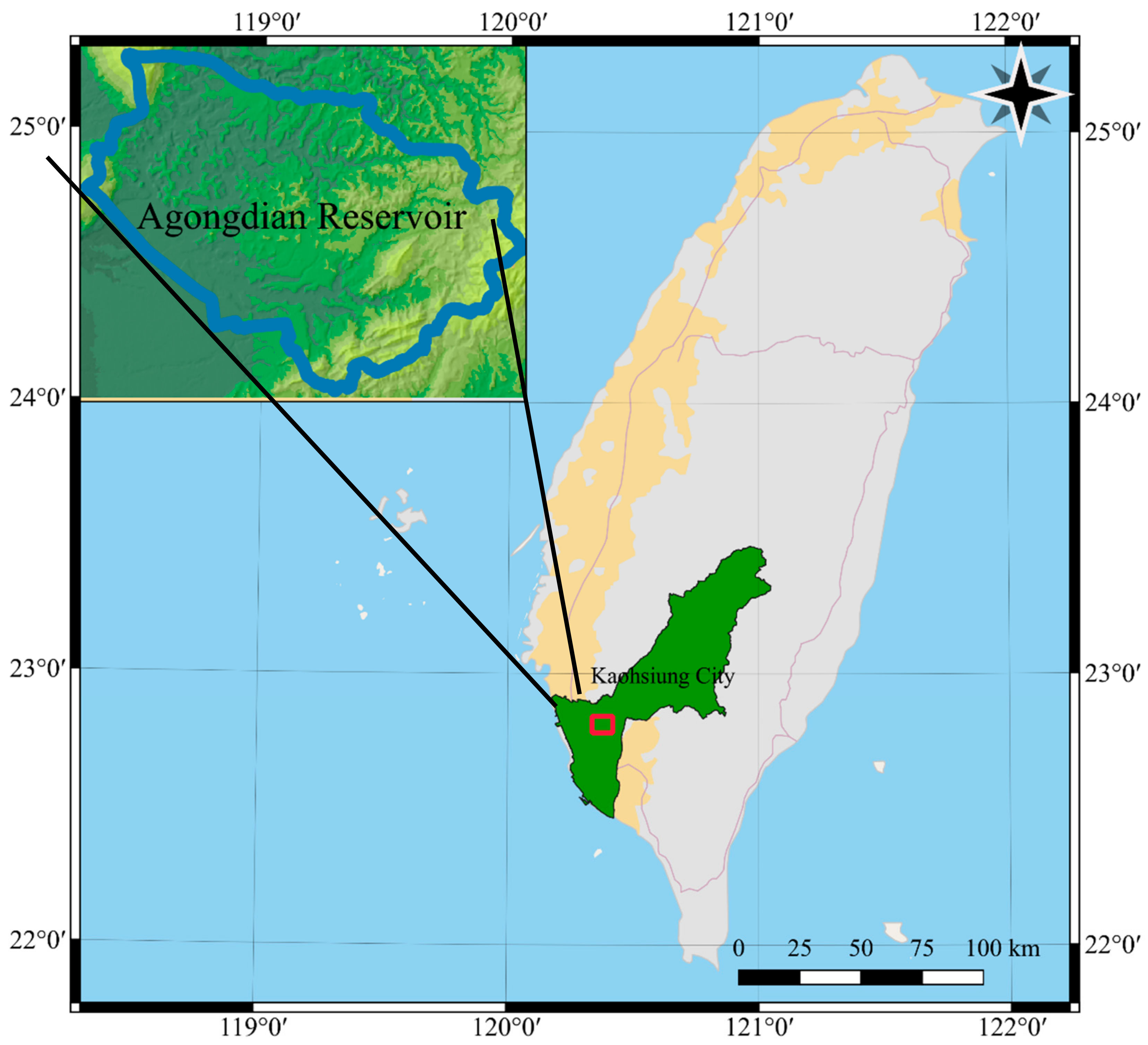
2.1. Soil Specimens and Geotechnical Tests

The soils used for the erosion experiments were collected from the watershed of Agongdian Reservoir in Kaohsiung city, which is located in southwestern Taiwan (Figure 1). The parent rock in the watershed belongs to green-gray mudstone, which melts easily when absorbing water; most of the top soils are weathered loam or sandy loam based on the USDA (U.S. Department of Agriculture) soil classification system. Due to the high percentage of fine sediments and the melting characteristic of mudstone, the soils are hardened when dry but easily eroded when subjected to continuous rainfall during storm events. In addition, the high content of salts of mudstone soils is not suitable for vegetation, and thus soil loss from hillslopes has led to environmental issues in the watershed, such as reservoir siltation.
After the soils were collected from the field, preliminary treatments, including air drying, gravels and plants picking, peds crumbling, and sieving through a 2-mm sieve, were carried out before the conventional geotechnical tests. As background information, the specific gravity and grain size distribution of the mudstone soils were determined before the erosion experiments by following procedures outlined in American Society for Testing and Materials (ASTM) standards, including ASTM D854-14 [26], ASTM C136/C136M-14 [27], ASTM D1140-14 [28], and ASTM D422-63-07 [29], referring to the pycnometer test, dry sieve analysis, wet sieve analysis, and hydrometer test, respectively. As the results indicate, the mudstone soils have an average specific gravity of 2.69 g/cm3 and consist of 52.15% of sand, 45.75% of silt, and 5.91% of clay on average, and belong to sandy loam based on the USDA soil classification system. The moisture content shows the ratio of pore water mass to the mass of dry solids, and was conducted following the ASTM D2216-10 [30] procedure. Before each trial of the erosion experiments, 24 soil specimens were sampled to estimate the spatial variation of moisture contents of the soils filled in the flume to determine the antecedent soil moisture condition. The soil specimens for soil moisture content measurements were sampled following the method for group B in the ASTM D4220/D4220M-14 [31] procedure. Based on [1,15], the soils were filled to the flume as three 0.05-m-thick layers, and eight soil specimens were sampled at an equal distance for each soil layer.

2.2. Sloping Flume Erosion Experiment

The experimental setup of the erosion experiment, including the rainfall simulator, the sloping flume, and the stripe laser apparatus, is shown in Figure 2. The flume is 0.75 m in length, 0.25 m in width, and 0.25 m in depth, and with an adjustable slope gradient range from 0° to 30°. Below the flume bottom, a plastic container was used to collect the infiltrated outflow and sediments during the erosion process. At the outlet of the flume, a funnel-shape opening was designed for collecting the outflow water and sediment yields. To minimize experimental uncertainty and obtain good controls on experimental factors, we carried out the erosion experiments and recorded the erosion topography using a small-scale rainfall simulator and a flume with adjustable slopes. The rainfall simulator, stripe laser apparatus, soil specimen preparation, and test procedure and measurements of the laboratory erosion experiment are described in the following subsections.

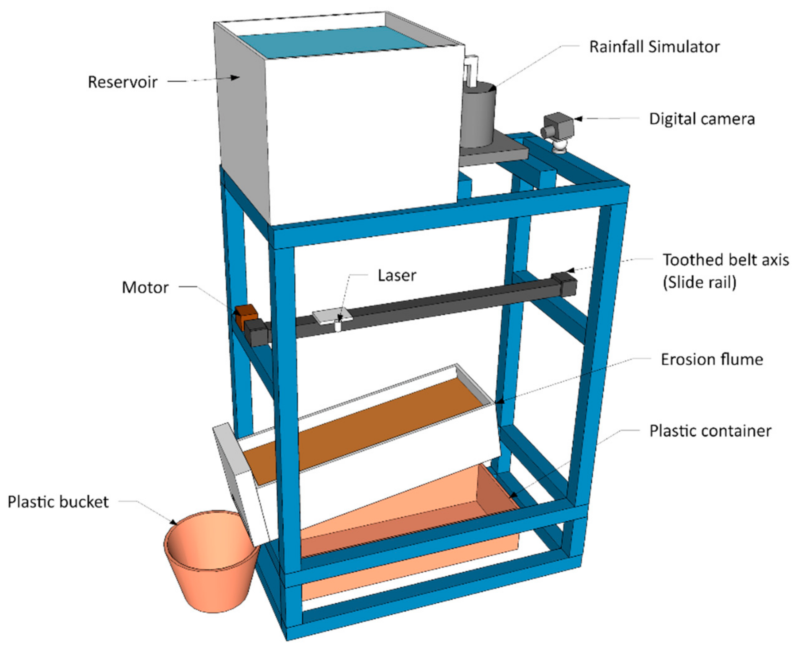
2.2.1. Rainfall Simulator

The mini rainfall simulator used for the erosion test is manufactured by Eijkelkamp Soil & Water (EM Giesbeek, the Netherlands) [32], with a rainfall area of 0.25 m × 0.25 m produced by 49 probes with a constant water head. Compared to natural precipitation, simulated rainfalls usually have a shorter falling distance, which results in a lower terminal velocity of rain drops and thus a smaller kinetic energy. This concept was described in the previous study, in which the same rainfall simulator of this study was applied [33]. Therefore, to compensate for the short falling distance of the simulated rainfall (ranging from 0.61 m to 0.69 m with the slope gradient ranging from 5° to 30°, which covered most of the slopes in the study area), the high intensity of the simulated rainfall was applied. From the equation of time-specific kinetic energy [34], the time-specific kinetic energy produced by the simulated rainfalls equals that of natural rainfall events with the intensity ranging from 76 mm/h to 84 mm/h when the slope varies from 5° to 30°. The rainfall simulator was located at the upstream side of the flume and generated simulated rainfalls covering the range of 0.25 m × 0.25 m. The remaining downstream region of the soil surface was used to observe rill development during the erosion process.

2.2.2. Stripe Laser Apparatus

The stripe laser apparatus used for obtaining erosion topographies consists of a 100-mW diode laser (FLEXPOINT® Machine Vision Lasers Mvnano Series, Olching, Germany), an electric slide rail (Igus drylin® ZLW, Köln, Germany), and a digital camera (Nikon D7200, Tokyo, Japan). By applying pattern projection methods [35], the projected single stripe of light onto the soil surface, which was produced by the diode laser moving with a constant speed along the flume on the electric slide rail, was recorded by the digital camera to reconstruct a whole surface from digital camera images. Detailed discussions of the stripe laser apparatus, the basic principles of the scan processing method, and scan resolution and error estimation are provided in previous studies [35,36]. The reconstruction of a scanned surface was achieved using the images of the stripe laser rays captured by the digital camera for each cross-section of the soil surface apart by 1 mm. The images were processed in the MATLAB (2017a, MathWorks Inc., Natick, MA, USA) program developed the previous study [36] and the erosion topographies were obtained.

2.2.3. Soil Specimen Preparation

For the soil specimen preparation of each erosion test, the air-dried and pretreated soils were mixed with tap water thoroughly by human force; then, the moisturized soil was placed in the storage container and the soil surface was covered and allowed to stand for at least 16 h as suggested by the wet preparation method in the ASTM D4318-10 procedure [37]. To target an antecedent soil moisture content around 20% and a bulk density of 1400 kg/m3, 39.375 kg of dried soil and 1.875 kg of tap water were used. The moisturized soils were filled by three layers, with each layer 0.05-m thick [1,15], and a total of 0.15 m in soil depth. After a layer was filled, soils sampled at the eight sites distributed in equal spaces were used to determine the actual antecedent soil moisture conditions. Therefore, a total of 24 soil specimens for the 3 filled soil layers were sampled to determine the average antecedent soil moisture content for each test of the erosion experiments. After the soils were filled in the flume, an initial laser scan was carried out through the soil surface to obtain the topography before the simulated rainfall [36]. Then, the flume was tilted by a screwing jack to a designed slope and the simulated rainfall began.

2.2.4. Test Procedure and Measurements

After a rainfall simulation began, the outflows of water and sediments were collected by the bottom container and the outlet bucket every 5 min until the end of the test. To collect infiltrations during experiments [38,39], the bottom container collected the infiltrated outflow in this study, while the outlet bucket collected the surface outflow. Then, the total sediment yield can be obtained as the summation of the sediments transported by the infiltrated and surface outflows. The collected outflows were dried in an oven at 105 °C for 24 h [1,15,40], and the remnant soils were weighed as the measurements of sediment yields. In this study, the collected sediment yields are considered as the “measured” soil loss. Meanwhile, to record the soil surface topography for each 5-min increment of the rainfall, the simulated rainfall was temporarily stopped for 20 min [17], the flume was lowered to the horizontal position, and the laser scan was carried out. The duration of each rainfall event was 30 min [15]. Therefore, seven laser-scanned topographies were obtained for a single rainfall event. To account for the effect of steepness on hillslope erosion, six slope gradients (5°, 10°, 15°, 20°, 25°, and 30°) were used in the experiments and two replicates [15] were applied for each gradient.

2.3. Erosion Volume Generation and Data Treatment

By applying the stripe laser-scanning technique, we obtained a DEM of the soil surface through each test of the scanning procedure at each time step. Then, the DEMs were subtracted on a cell-by-cell basis to obtain the difference of depths throughout the whole soil surface. The soil volume differences among the erosion topographies were obtained; then, the mass of soil loss can be estimated by the soil volume differences, the moisture content, and the bulk density of the soil. The resultant soil loss in mass is considered to be the “estimated” soil loss. Since the computation of the difference of depths from two DEMs can propagate the errors of the initial DEMs [16,35,36], we applied an error analysis by comparing the elevation precision using check points on the soil surface of the laser-scanned DEMs to determine the minimum level of detection for the depth difference. The error in depth difference of two DEMs was estimated as the quadratic composition of errors [35,36] in each of the original DEMs being compared [16], and it can be calculated as:
E d o d _ i = E D E M _ i 2 + E D E M _ i + 1 2
where E d o d _ i means the error of depth difference between two DEMs of the erosion experiments; E D E M _ i   means the error of the DEM at time step i calculated from the check points calibration; and E D E M _ i + 1   means the error of the DEM at time step i + 1 calculated from the check points calibration. For the erosion experiments, the detection threshold for the depth differences between two DEMs was set as the E d o d value. From the calibrations and error analyses of the check points, the minimum value of E d o d [16] was 1.28 mm. Therefore, a difference of depths was accounted for in the calculation of a soil volume difference between two DEMs when its absolute value is ≥1.28 mm.

3. Results

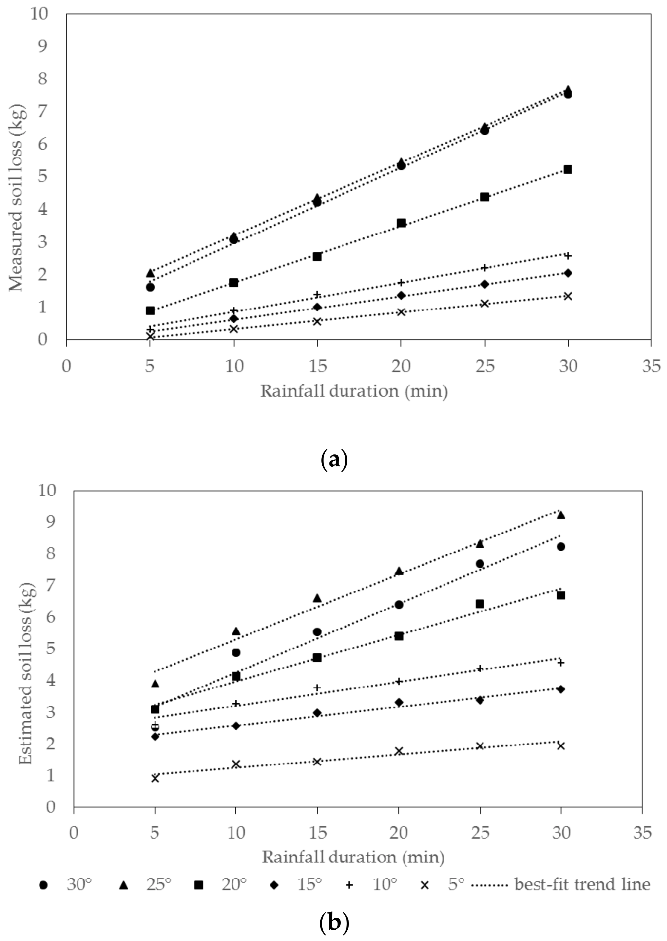
3.1. Soil Loss Measured by the Sediment Yields

During a test of a 30-min simulated rainfall event, the sediment yield was collected every 5 min until the end of the test, and the cumulative sediment yields are shown in Table 1. The cumulative sediment yields increase with the rainfall duration, and the total sediment yields at the end of the test range from 1.228 kg to 8.300 kg of oven-dried soil mass. Based on the infiltrated outflow collected by the plastic container below the flume bottom during the erosion experiments, outflows of infiltrated sediments occurred in the tests with 5°, 10°, and 15° of slopes but not in the tests with steeper slopes. On average, the cumulative infiltrated sediment outflows account for 18.4% of the total cumulative sediment yields after the 30-min rainfall events.

3.2. Soil Loss Estimated by the Laser-Scanned Soil Volume Differences

From the differences of depths generated by the subtraction of any two DEMs (with a spatial resolution of 1 mm × 1 mm), the soil volume differences were calculated by summing up all the depth difference values exceeding the detection threshold. Then, the estimated soil loss in mass, the volume-difference soil loss, was the product of the soil volume difference and the soil bulk density resulting from the average soil moisture contents. During a test of a 30-min simulated rainfall event, the volume-difference soil loss was obtained every 5 min until the end of the test, and the cumulative volume-difference soil loss is shown in Table 2. The cumulative volume-difference soil loss increases with the rainfall duration, and the total volume-difference soil loss at the end of the test ranges from 1.833 kg to 10.775 kg. From observations during the experiments, the depression of the soil surface under rain drop compaction and collapse along the side-wall of rills were the main factors for overestimates in the soil loss, especially during the first 5 min of the rainfalls.

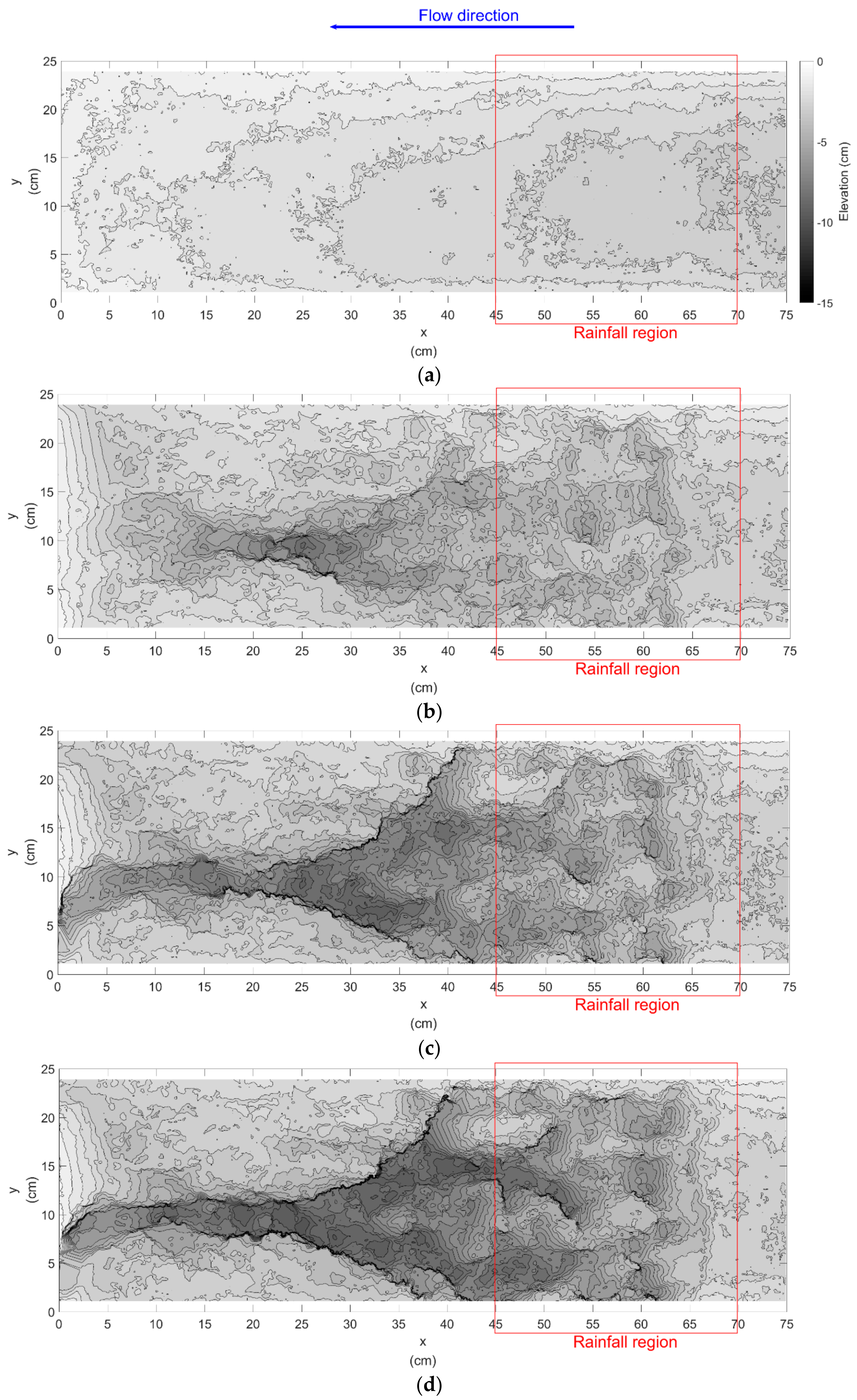
3.3. Laser-Scanned Topographies during Erosion

For each test of the simulated rainfall erosion experiment, seven laser-scanned topographies, including the initial soil surface topography, were carried out. As an example, the laser scanner topographies of the erosion test with a 30° slope are shown in Figure 3. From the soil surface topographies, the propagation of erosion processes can be described qualitatively. In Figure 3, an increase in the soil surface depression areas suggested soil erosion propagation caused by rain drop compaction/rain splash erosion, sheet flow erosion, and sediment entrainment of concentrated flows. Specifically, rain drop compaction occurred in the rainfall region at 45 cm to 70 cm from the outlet; erosion of the overland sheet flow occurred in the rainfall region and the middle stream area around x = 30 cm to x = 45 cm during the first 10 min of the rainfall, and then the formation of rills was observed as the effect of rill erosion. In the area with a distance from the outlet less than 30 cm, the main erosion process was sediment entrainment of the concentrated flows. The depths of the eroded channel for the concentrated flow in x = 0 to x = 30 increased with the rainfall duration, which are shown in Figure 3b–f. However, comparison between Figure 3f,g suggests that deposition occurred in the region of x = 0 to x = 15 during the last 5 min of the rainfall event, which may be caused by collapse of the rill sides during sediment entrainments or the outflow being too small and plugged.

4. Discussion

4.1. Effects of Rainfall Duration and Slope on Soil Loss

Effects of rainfall duration and slope on the soil loss mass are illustrated in Figure 4. From the figure, the mass of the soil loss, both measured from the sediment yields and estimated from the soil volume differences, increased with the rainfall duration and the slope. From previous studies [41,42], similar results have been proposed regarding the positive correlation between rainfall or constant flow duration and the eroded soil volume quantified by rill dimensions. Under a constant rainfall intensity, the increase in rainfall duration suggests the increase of cumulative kinetic energy provided by rain drop compaction and the surface flow, which thus results in a larger eroded soil volume and mass of soil loss [41,42]. The increase of soil loss with slope has also been presented in many previous studies [2,15,43], which may be attributed to the decrease of soil particle stability as the slope increases [44].
In Figure 4, the slopes of the trend lines decreased from 0.22 to 0.04 as the slope gradient of the flume decreased from 30° to 5°, indicating that the effect of the topography on soil loss became less significant in cases of mild slopes. In other words, the effect of rainfall duration on the soil loss mass can be influenced by the slope, and thus a collective effect of the rainfall duration and the slope on the soil loss should be considered. We applied a multiple regression analysis to quantify the effects of rainfall duration, slope, and their product term (to account for the collective effect of rainfall duration and slope) on the measured/estimated soil loss in mass, and the equations are as follows:
S L m = 0.023 t + 0.018 S + 0.009 ( S × t ) R 2 = 0.96
S L e = 0.048 t + 0.112 S + 0.005 ( S × t )   R 2 = 0.96
where S L m = measured soil loss in mass (kg); S L e = estimated soil loss in mass (kg); S = slope of the flume (°); t = rainfall duration (min). In Equations (2) and (3), positive coefficients before the product terms ( S × t ) suggest that the positive effects of rainfall duration on soil loss manifested as the slope increased.

4.2. Relation between the Estimated and Measured Soil Loss

In Figure 5, data of the estimated soil loss, calculated based on the soil volume difference between two DEMs, are plotted versus the measured soil loss, which comprised the sediment yields collected during the experiments. The data points located above the 1:1 line suggest a systematic overestimation, which might occur within the first 5 min of rainfalls for all of the cases. Soil compaction and surface depression caused by the impact of rain drops might be the main reason for the overestimated soil loss. After the compaction of the surface soil stopped when the large soil pores collapsed, the soil volume difference increased as soil erosion propagated and more soil particles were eroded and transported to the flume outlet. The linear relation between the estimated soil loss ( S L e ) and the measured soil loss ( S L m ) shown in Equation (4) suggests a similar increasing rate in S L e with S L m by the trend line slope close to unity. The positive intercept in Equation (4) indicates an overestimation in soil loss resulting from soil compaction and effects of heterogeneity in soil structure and soil density or moisture content.
S L e =   0.98 S L m + 1.73   R 2 = 0.91
For application, the best-fit least square trend line is proposed by plotting the measured cumulative soil loss versus the soil volume differences subtracted from two DEMs, which were obtained by the stripe laser-scanned topographies, and the equation is:
S L m =   1281.9 V 1.36   R 2 = 0.91
where V means the eroded soil volume (m3) calculated as the soil volume differences subtracted from two DEMs. From Equation (5), the overestimation of soil volume differences due to soil compaction by rain drops was accounted for and offset by the negative intercept. Therefore, once an eroded soil volume can be obtained, the soil loss in mass may be predicted using Equation (5).

4.3. Erosion Processes and Rill Developlemt

Different types of soil erosion were reviewed, including splash erosion, sheet flow (interrill) erosion and rill erosion, and sediment transport of flow [45]. Based on the descriptions and characteristics of the soil erosion types [45], we classified the erosion processes for the case of the 30° slope erosion test shown in Figure 3. From the soil surface topographies in Figure 3, we quantified the estimated soil loss from soil volume differences for three cross sections in the flume following the descriptions of the laser-scanned topographies in Section 3.3, which are 45–70 cm (the rainfall region), 30–45 cm, and 0–30 cm from the outlet, to show the percentages of soil loss attributed to different erosion processes. From Table 3, the rain drop compaction and rain splash erosion that occurred in the rainfall area (45 cm to 70 cm from the outlet) accounted for 23% to 33% of the estimated total soil loss as the rainfall duration increased. However, the soil surface depression observed during the experiments suggested that the larger volumetric soil differences resulted from soil surface depression and compaction by the rain drops in addition to the actual soil loss by rain splash erosion; this is considered to be the main source of error for overestimations of the measured soil loss. The region of 30 cm to 45 cm from the outlet provided 28% to 33% of the estimated total soil loss. In this region, sheet erosion and interill erosion of the overland flow were observed as the dominant erosion processes during the first 10 min. Afterwards, rill erosion became more significant as rills developed. In the region close to the outlet (x = 0 cm to x = 30 cm), sediment entrainment by the concentrated flow in the rills was the dominant erosion process, and it provided 34% to 49% of the estimated total soil loss. While the transitions among different erosion processes were observed during the experiments and judged based on the laser-scanned topographies, more experiments designed for observing each erosion type and relative further studies are desired to validate the quantitative descriptions of the erosion process propagation.
From Figure 3, the development of a rill can be observed with the propagation of erosion processes and be described qualitatively. Specifically, the areas with dense contours suggest an incision in the soil surface and the development of rills. For the case of the 30° slope erosion test (Figure 3b), the initiation of the rill occurred at x = 20 cm to x = 30 cm where the concentrated flow was formed on the soil surface, which was around 20 cm apart from the lower boundary of the rainfall region (i.e., x = 45 cm), after 5 min of rainfall. Afterwards, the development of the dendritic structure indicated by the dense contours in Figure 3c–g suggested that the rill continuously developed upstream by headcutting towards the rainfall region as the rainfall duration increased. Meanwhile, the concentrated flow eroded the soil surface continuously towards the outlet and resulted in a deep and wide main stream in the region of x = 0 cm to x = 30 cm. Critical conditions for rill initiation were studied [46]. They proposed that headcutting occurred following rill formation and thus the upper ends of the rills were not the exact positions of rill initiation. While the rill development process observed in this study was similar to that reported in the literature [46], further research is required to obtain quantified evaluations of rill network development and the effects of topographic factors, such as slope.

5. Conclusions

In this study, erosion processes on a small-scale soil surface were observed and evaluated by erosion experiments using an adjustable slope flume, a rainfall simulator, and a stripe laser-scanning apparatus. From the results, the effects of rainfall duration, slope, and the combined influences of the two factors on the measured/estimated soil loss mass were quantified by Equations (2) and (3), suggesting that the positive effects on soil loss of rainfall duration were manifested as the slope increased. By comparing the measured and the estimated soil loss, Equation (4), with the slope near to unity and the R2 value of 0.91, indicates good agreements between the soil loss measurements and the estimations. The stripe laser-scanning method was applied successfully to evaluate soil loss by subtracting the DEMs generated from scanned topographies. In practice, Equation (5) suggests that soil loss can be predicted by the soil volume differences between two DEMs given information of soil bulk density/moisture content and the soil compaction by rain drops.
From the laser-scanned soil surface topographies, the propagation of erosion processes and development of rills can be described qualitatively. From the case of the 30° slope erosion experiment, erosion processes, including rain drop compaction and rain splash erosion, sheet erosion, interrill erosion, and rill erosion, were observed. Based on the observation, the initiation of a rill occurred around 20 cm apart from the lower boundary of the rainfall region after 5 min of rainfall and progressed both upstream and downstream as the rainfall continued. This phenomenon coincides with the headcutting reported in the literature [46]. While more experiments and further studies are desired to obtain a whole picture of erosion process propagation and rill development during rainfall events, the results in this study provide: (1) quantified equations to predict soil loss by rainfall duration and slope and by eroded soil volume from DEM data; and (2) a potential method to quantitatively evaluate an erosion process in laboratory-scale experiments.

Author Contributions

Y.-C.W. conceived and designed the experiments; C.-C.L. performed the experiments; Y.-C.W. and C.-C.L. analyzed the data; Y.-C.W. wrote the paper.

Funding

The authors would like to thank the Ministry of Science and Technology, and the Soil and Water Conservation Bureau of the Republic of China, Taiwan, for financially supporting this research under the Contract No. 106-2625-M-005-013 and the Report No. SWCB-107-042, respectively.

Acknowledgments

The authors would like to thank Chi-Yao Hung, who is currently a faculty member in the Department of Soil and Water Conservation, National Chung Hsing University, Taiwan, and provided professional advice and technical support for the stripe laser-scanning method and DEM data transformation.

Conflicts of Interest

The authors declare no conflict of interest.

References

  1. Shen, H.; Zheng, F.; Wen, L.; Lu, J.; Jiang, Y. An experimental study of rill erosion and morphology. Geomorphology 2015, 231, 193–201. [Google Scholar] [CrossRef]
  2. Chen, X.-Y.; Zhao, Y.; Mi, H.-X.; Mo, B. Estimating rill erosion process from eroded morphology in flume experiments by volume replacement method. Catena 2016, 136, 135–140. [Google Scholar] [CrossRef]
  3. Meyer, L.D.; Foster, G.R.; Romkens, M.J.M. Source of soil eroded by water from upland slopes. In Present and Prospective Technology for Predicting Sediment Yields and Sources, Proceedings of the Sediment-Yield Workshop, Oxford, MS, USA, 28–30 November 1972; pp. 177–189.
  4. Mutchler, C.K.; Young, R.A. Soil detachment by raindrops. In Present and Prospective Technology for Predicting Sediment Yields and Sources, Proceedings of the Sediment-Yield Workshop, Oxford, MS, USA, 28–30 November 1972; pp. 113–117.
  5. Zhang, P.; Tang, H.; Yao, W.; Zhang, N.; Xizhi, L.V. Experimental investigation of morphological characteristics of rill evolution on loess slope. Catena 2016, 137, 536–544. [Google Scholar] [CrossRef]
  6. Boardman, J. Soil erosion science: Reflections on the limitations of current approaches. Catena 2006, 68, 73–86. [Google Scholar] [CrossRef]
  7. Moreno-de Las Heras, M.; Espigares, T.; Merino-Martín, L.; Nicolau, J.M. Water-related ecological impacts of rill erosion processes in Mediterranean-dry reclaimed slopes. Catena 2011, 84, 114–124. [Google Scholar] [CrossRef]
  8. Lei, T.W.; Zhang, Q.; Zhao, J.; Tang, Z. A laboratory study of sediment transport capacity in the dynamic process of rill erosion. Am. Soc. Agric. Eng. 2001, 44, 1537–1542. [Google Scholar]
  9. Lawrence, W.; Gatto, L.W. Soil freeze-thaw-induced changes to a simulated rill: Potential impacts on soil erosion. Geomorphology 2000, 32, 147–160. [Google Scholar]
  10. Dong, Y.Q.; Zhuang, X.H.; Lei, T.W.; Yin, Z.; Ma, Y.Y. A method for measuring erosive flow velocity with simulated rill. Geoderma 2014, 232–234, 556–562. [Google Scholar] [CrossRef]
  11. Bewket, W.; Sterk, G. Assessment of soil erosion in cultivated fields using a survey methodology for rills in the Chemoga watershed, Ethiopia. Agric. Ecosyst. Environ. 2003, 97, 81–93. [Google Scholar] [CrossRef]
  12. Aksoy, H.; Unal, N.E.; Cokgor, S.; Gedikli, A.; Yoon, J.; Koca, K.; Inci, S.B.; Eris, E. A rainfall simulator for laboratory-scale assessment of rainfall-runoff-sediment transport processes over a two-dimensional flume. Catena 2012, 98, 63–72. [Google Scholar] [CrossRef]
  13. Zheng, F.L. A research on method of measuring rill erosion amount. Bull. Soil Water Conserv. 1989, 9, 41–49. [Google Scholar]
  14. Casalí, J.; Loizu, J.; Campo, M.A.; De Santisteban, L.M.; Álvarez-Mozos, J. Accuracy of methods for field assessment of rill and ephemeral gully erosion. Catena 2006, 67, 128–138. [Google Scholar] [CrossRef]
  15. Shen, H.; Zheng, F.; Wen, L.; Han, Y.; Hu, W. Impacts of rainfall intensity and slope gradient on rill erosion processes at loessial hillslope. Soil Tillage Res. 2016, 155, 429–436. [Google Scholar] [CrossRef]
  16. Balaguer-Puig, M.; Marqués-Mateu, Á.; Lerma, J.L.; Ibáñez-Asensio, S. Estimation of small-scale soil erosion in laboratory experiments with Structure from Motion photogrammetry. Geomorphology 2017, 295, 285–296. [Google Scholar] [CrossRef]
  17. Berger, C.; Schulze, M.; Rieke-Zapp, D.; Schlunegger, F. Rill development and soil erosion: A laboratory study of slope and rainfall intensity. Earth Surf. Proc. Land. 2010, 35, 1456–1467. [Google Scholar] [CrossRef]
  18. Heng, B.C.P.; Chandler, J.H.; Armstrong, A. Applying close range digital photogrammetry in soil erosion studies. Photogramm. Rec. 2010, 25, 240–265. [Google Scholar] [CrossRef] [Green Version]
  19. Nouwakpo, S.; Huang, C.-H.; Frankenberger, J.; Bethel, J. A simplified close range photogrammetry method for soil erosion assessment. In Proceedings of the 2nd Joint Federal Interagency Conference, Las Vegas, NV, USA, 27 June–1 July 2010. [Google Scholar]
  20. Vinci, A.; Brigante, R.; Todiscoa, F.; Mannocchi, F.; Radicioni, F. Measuring rill erosion by laser scanning. Catena 2015, 124, 97–108. [Google Scholar] [CrossRef]
  21. Afana, A.; Solé-Benet, A.; Pérez, J.L. Determination of soil erosion using laser scanners. In Proceedings of the 19th World Congress of Soil Science, Soil Solutions for a Changing World, Brisbane, Australia, 1–6 August 2010. [Google Scholar]
  22. Longoni, L.; Papini, M.; Brambilla, D.; Barazzetti, L.; Roncoroni, F.; Scaioni, M.; Ivanov, V.I. Monitoring riverbank erosion in mountain catchments using terrestrial laser scanning. Remote Sens. 2016, 8, 241. [Google Scholar] [CrossRef] [Green Version]
  23. Dąbek, P.B.; Patrzałek, C.; Ćmielewski, B.; Żmuda, R. The use of terrestrial laser scanning in monitoring and analyses of erosion phenomena in natural and anthropogenically transformed areas. Cogent Geosci. 2018, 4, 1437684. [Google Scholar] [CrossRef]
  24. Thoma, D.P.; Gupta, S.C.; Bauer, M.E.; Kirchoff, C.E. Airborne laser scanning for riverbank erosion assessment. Remote Sens. Environ. 2005, 95, 493–501. [Google Scholar] [CrossRef]
  25. Filin, S.; Baruch, A.; Morik, S.; Avni, Y.; Marco, S. Characterization of land degradation processes using airborne laser scanning. In Proceedings of the International Archives of the Photogrammetry, Remote Sensing and Spatial Information Science, Kyoto, Japan, 9–12 August 2010. [Google Scholar]
  26. ASTM. Standard Test Methods for Specific Gravity of Soil Solids by Water Pycnometer; D854-14; ASTM: West Conshohocken, PA, USA, 2014. [Google Scholar]
  27. ASTM. Standard Test Method for Sieve Analysis of Fine and Coarse Aggregate; ASTM C136/C136M-14; ASTM: West Conshohocken, PA, USA, 2015. [Google Scholar]
  28. ASTM. Standard Test Methods for Determining the Amount of Material Finer than 75-μm (No. 200) Sieve in Soils by Washing; D1140-14; ASTM: West Conshohocken, PA, USA, 2014. [Google Scholar]
  29. ASTM. Standard Test Method for Particle-Size Analysis of Soils; ASTM D422-63; ASTM: West Conshohocken, PA, USA, 2007. [Google Scholar]
  30. ASTM. Standard Test Methods for Laboratory Determination of Water (Moisture) Content of Soil and Rock by Mass; D2216-10; ASTM: West Conshohocken, PA, USA, 2010. [Google Scholar]
  31. ASTM. Standard Practices for Preserving and Transporting Soil Samples; D4220/D4220M-14; ASTM: West Conshohocken, PA, USA, 2014. [Google Scholar]
  32. Eijkelkamp Soil & Water. Available online: https://en.eijkelkamp.com/products/field-measurement-equipment/rainfall-simulator.html (accessed on 3 July 2018).
  33. Nciizah, A.D.; Wakindiki, I.I.C. Rainfall pattern effects on crusting, infiltration and erodibility in some South African soils with various texture and mineralogy. Water SA 2014, 40, 57–64. [Google Scholar] [CrossRef]
  34. Salles, C.; Poesen, J.; Sempere-Torres, D. Kinetic energy of rain and its functional relationship with intensity. J. Hydrol. 2002, 257, 256–270. [Google Scholar] [CrossRef]
  35. Hung, C.-Y.; Capart, H. Rotating laser scan method to measure the transient free-surface topography of small-scale debris flows. Exp. Fluids 2013, 54, 1544. [Google Scholar] [CrossRef]
  36. Hung, C.-Y. Relation between Debris Flow Rheology and Fan Deposit Morphology Investigated Using Small-Scale Experiments. Master’s Thesis, National Taiwan University, Taipei, Taiwan, June 2011. [Google Scholar]
  37. ASTM. Standard Test Methods for Liquid Limit, Plastic Limit, and Plasticity Index of Soils; D4318-10; ASTM: West Conshohocken, PA, USA, 2010. [Google Scholar]
  38. Bu, C.-F.; Wu, S.-F.; Yang, K.-B. Effects of physical soil crusts on infiltration and splash erosion in three typical Chinese soils. Int. J. Sediment Res. 2014, 29, 491–501. [Google Scholar] [CrossRef]
  39. Di Prima, S.; Concialdi, P.; Lassabatere, L.; Angulo-Jaramillo, R.; Pirastru, M.; Cerdà, A.; Keesstra, S. Laboratory testing of Beerkan infiltration experiments for assessing the role of soil sealing on water infiltration. Catena 2018, 167, 373–384. [Google Scholar] [CrossRef]
  40. Lin, L.-L.; Tung, H.-P.; Wan, H.-S. Handbook of Soil Physics Experiments; Department of Soil and Water Conservation, National Chung Hsing University: Taichung City, Taiwan, 2002. [Google Scholar]
  41. Shen, H.O.; Zheng, F.L.; Wen, L.L.; Lu, J.; Han, Y. An experimental study on rill morphology at loess hillslope. Acta Ecol. Sin. 2014, 34, 5514–5521. [Google Scholar] [CrossRef]
  42. Niu, Y.B.; Gao, Z.L.; Li, Y.H.; Luo, K.; Yuan, X.H.; Du, J.; Zhang, X. Rill morphology development of engineering accumulation and its relationship with runoff and sediment. Trans. Chin. Soc. Agric. Eng. 2016, 32, 154–161. [Google Scholar]
  43. He, J.-J.; Lu, Y.; Gong, H.-L.; Cai, Q.-G. Experimental study on rill erosion characteristics and its runoff and sediment yield process. Shuili Xuebao 2013, 44, 398–405. [Google Scholar]
  44. Chen, J.J.; Sun, L.Y.; Cai, C.F.; Liu, J.T.; Cai, Q.G. Rill erosion on different soil slopes and their affecting factors. Acta Pedol. Sin. 2013, 50, 281–288. [Google Scholar]
  45. Liu, Q.Q.; Li, J.C.; Chen, L.; Xiang, H. Dynamics of overland flow and soil erosion (II): Soil erosion. Adv. Mech. 2004, 34, 493–506. [Google Scholar]
  46. Yao, C.; Lei, T.; Elliot, W.J.; McCool, D.K.; Zhao, J.; Chen, S. Critical conditions for rill initiation. Trans. ASABE 2008, 51, 107–114. [Google Scholar] [CrossRef]
Figure 1. Map of the Agongdian Reservoir watershed in Kaohsiung city, Taiwan.
Water 10 00956 g001
Figure 2. Setup of the sloping flume erosion experiment.
Water 10 00956 g002
Figure 3. The laser-scanned topographies during the simulated rainfall erosion test of a 30° slope: (a) the initial topography before the rainfall started; the erosion topographies after (b) 5 min; (c) 10 min; (d) 15 min; (e) 20 min; (f) 25 min; and (g) 30 min of rainfall.
Water 10 00956 g003aWater 10 00956 g003b
Figure 4. Cumulative mass of soil erosion obtained by: (a) the cumulative sediment yields as the measured soil loss; (b) the cumulative volume-differences soil loss as the estimated soil loss.
Water 10 00956 g004
Figure 5. Estimated soil loss versus measured soil loss.
Water 10 00956 g005
Table 1. Sediment yield measurements collected at the outlet of the flume.
IndexCumulative Sediment Yield b (kg)
SlopeRainfall Duration (min)
51015202530
30° (1) a1.8023.3354.4045.5466.9238.3
30° (2) a1.4712.8154.065.1495.9486.766
25° (1)1.8292.984.0524.9465.7146.439
25° (2)2.2873.4224.6875.9757.3828.919
20° (1)1.0181.9372.8163.7994.4845.376
20° (2)0.8021.6042.3153.3964.2895.086
15° (1)0.1730.6951.1951.682.0992.46
15° (2)0.2850.5960.8361.0621.3341.646
10° (1)0.1670.6751.1081.3951.752.071
10° (2)0.4671.1161.6782.152.7083.1
5° (1)0.0880.3030.5040.9031.2131.507
5° (2)0.1180.3740.6460.8071.0651.228
Note: a (1) and (2) refers to the first and the second erosion test of each slope gradient, respectively. b Sediment yield = sediment outflow collected by the outlet bucket + infiltrated sediment outflow collected by the bottom container.
Table 2. Estimates of soil loss using laser-scanned topographies.
IndexCumulative Volume-Difference Soil Loss (kg)
SlopeRainfall Duration (min)
51015202530
30° (1) a3.1005.0586.0877.3678.5409.518
30° (2)1.9814.7064.9905.4436.8806.992
25° (1)3.8365.0125.8206.8137.0817.725
25° (2)3.9826.1207.4078.1239.59410.775
20° (1)3.0804.4145.0745.6526.8226.798
20° (2)3.1133.8544.3975.1766.0576.593
15° (1)2.6303.2063.5534.0254.1144.552
15° (2)1.8311.9472.4182.6302.6612.917
10° (1)2.9373.4324.0974.1064.5684.740
10° (2)2.3273.1433.4713.8774.2164.403
5° (1)0.9791.3941.3741.8612.0302.082
5° (2)0.8581.3821.5201.6981.8621.833
Note: a (1) and (2) refers to the first and the second erosion test of each slope gradient, respectively.
Table 3. Soil loss percentage of regions with different distances from the outlet: results of the erosion test with a 30° slope.
IndexSoil Loss Percentage to the Total Soil Loss
Rainfall Duration (min)Distance from the Outlet
45–70 cm30–45 cm0–30 cm
523%28%49%
1025%32%43%
1529%32%39%
2032%31%37%
2533%31%36%
3033%33%34%

