Toward a Weather-Based Forecasting System for Fire Blight and Downy Mildew


Abstract
1. Introduction
2. Experiments
2.1. Weather-Based System Design
2.2. HRES Data
2.3. Agrometeorological Observations
2.4. Disease Observation
3. Results
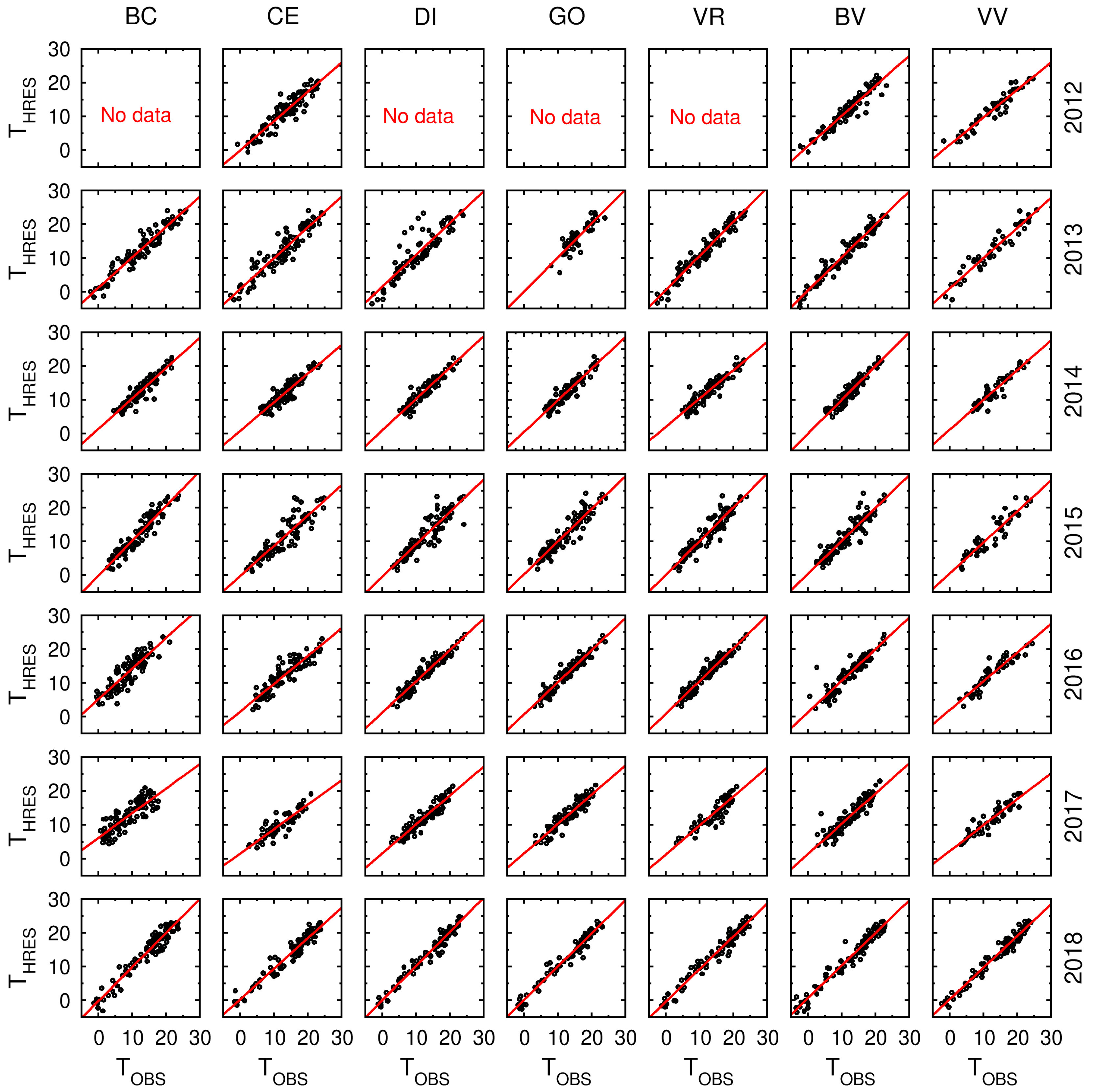
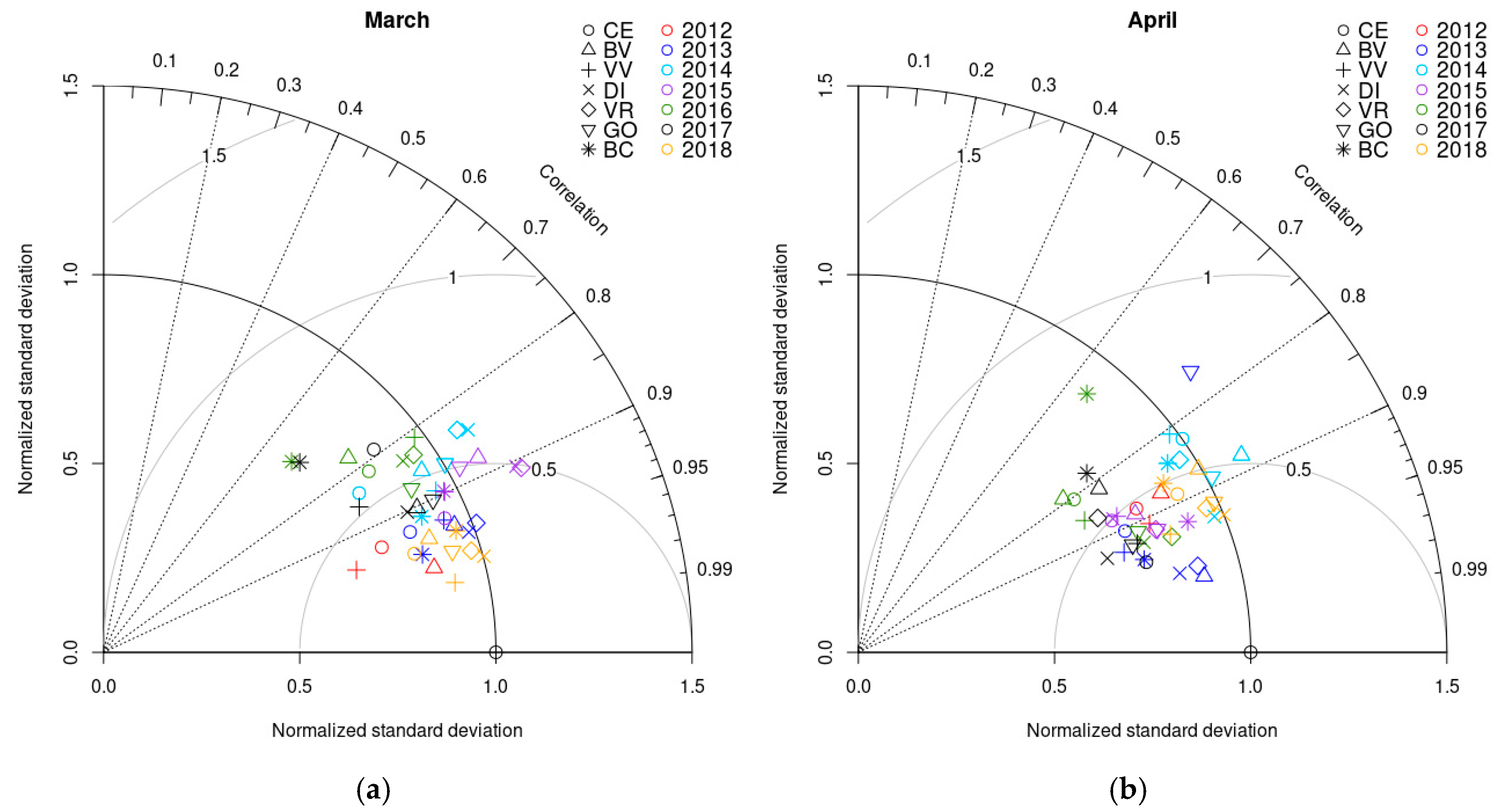
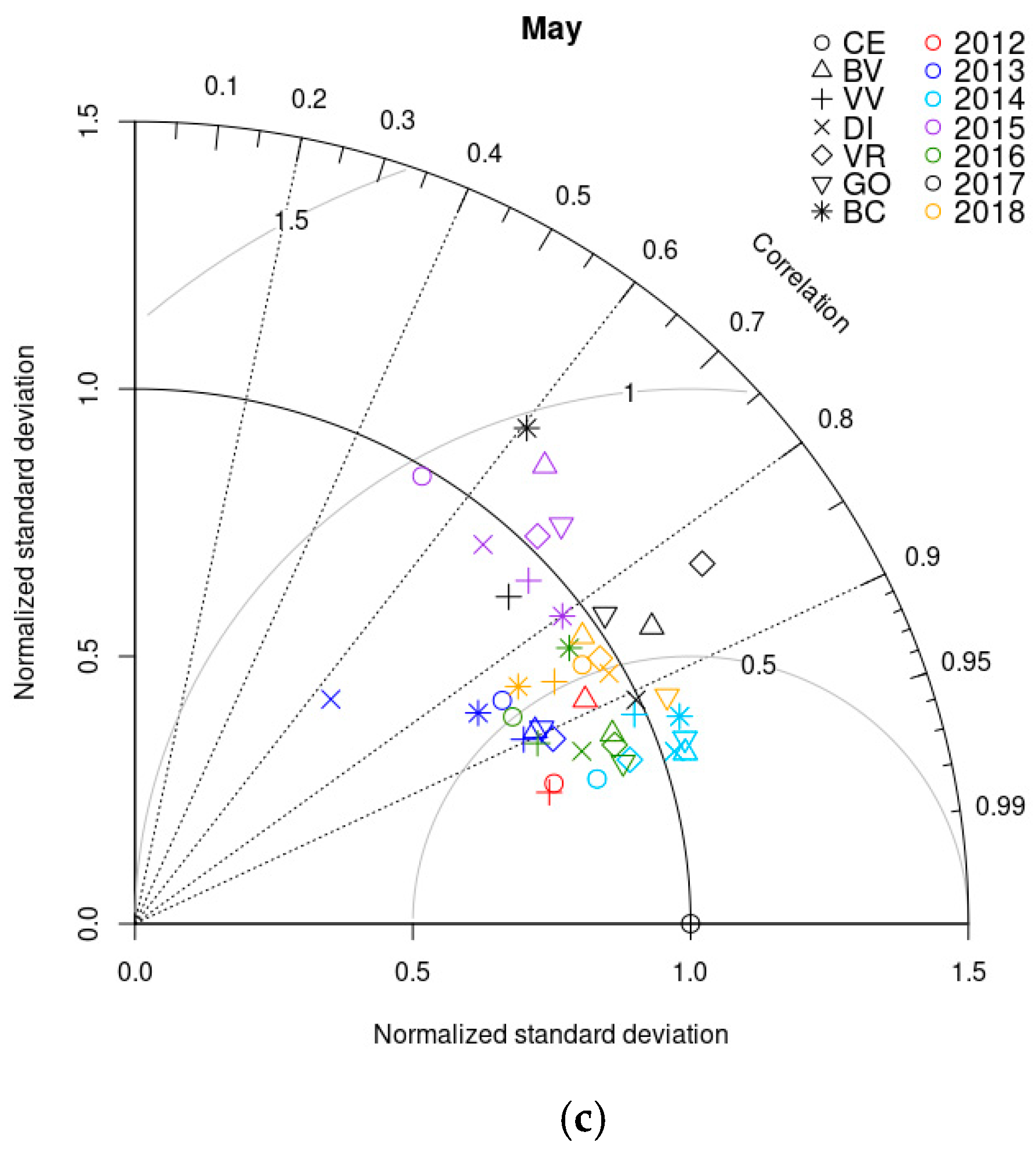
3.1. HRES Outputs
3.2. BAHUS Simulation Results
3.2.1. Downy Mildew, BAHUS-P
3.2.2. Fire Blight, BAHUS-E
4. Discussion
5. Conclusions
- -
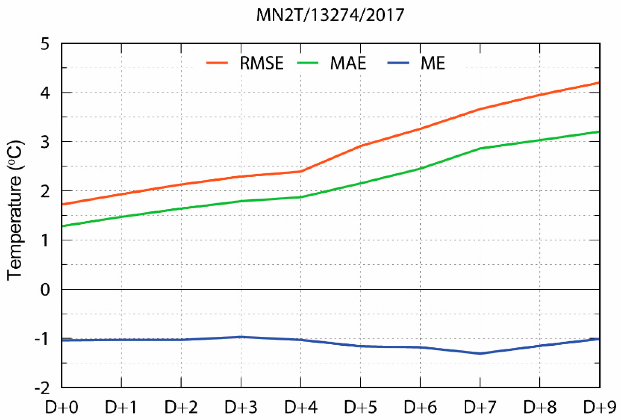
- The results for March–May in 2012–2018 at seven locations showed the high quality of the predicted temperature for the fifth day.
- -
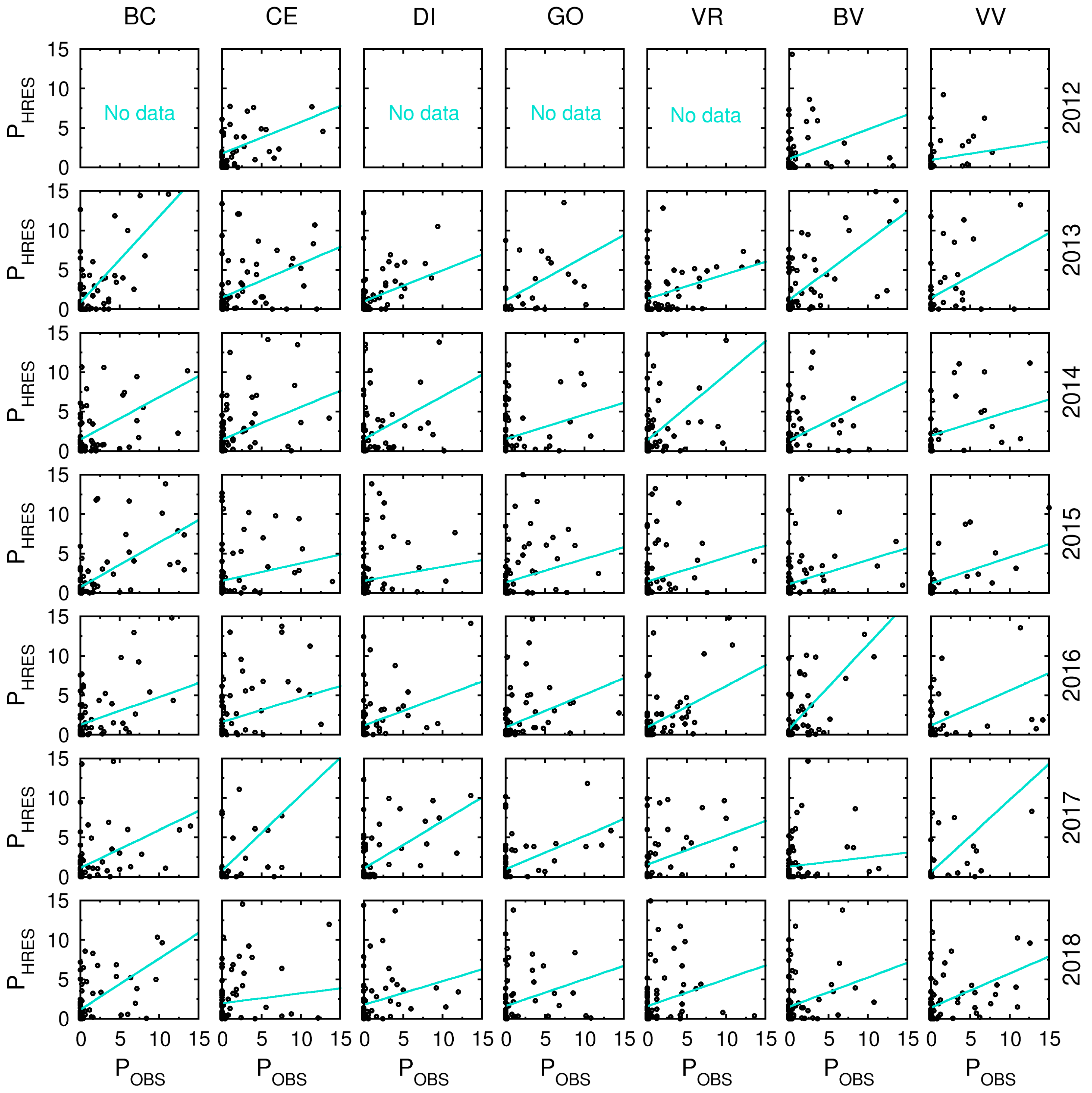
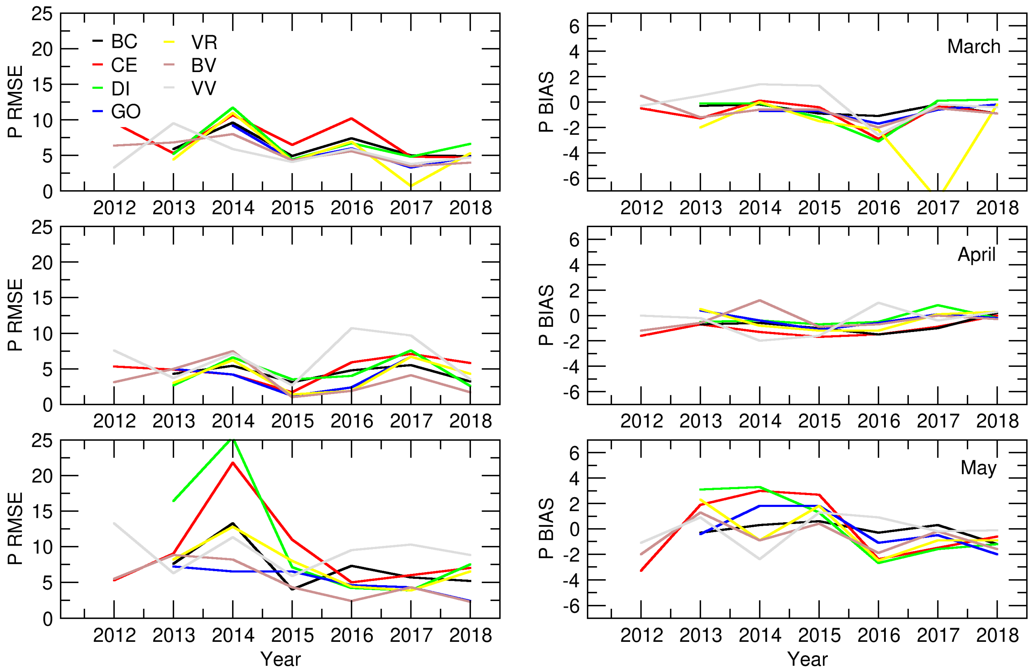
- The temperature-driven algorithms in BAHUS performed very well; the predicted amount of daily precipitation had errors, since it was the fifth day of the forecast and the uncertainties associated with precipitation were high.
- -
- The large errors in the daily sum of precipitation did not affect BAHUS results significantly, since both disease algorithms require the sum of precipitation over the threshold value for two days.
Supplementary Materials
Author Contributions
Funding
Acknowledgments
Conflicts of Interest
Appendix A


References
- Burruano, S. The life-cycle of Plasmopara viticola, cause of downy mildew of vine. Mycologist 2000, 14, 179–182. [Google Scholar] [CrossRef]
- Lafon, R.; Clerjeau, M. Downy mildew. In Compendium of Grape Diseases; Pearson, R.C., Goheen, A.C., Eds.; APS Press: St. Paul, MN, USA, 1988; pp. 11–13. [Google Scholar]
- Wong, F.P.; Burr, H.N.; Wilcox, W.F. Heterotallism in Plasmopara viticola. Plant Pathol. 2001, 50, 427–432. [Google Scholar] [CrossRef]
- Galbiati, C.; Longhin, G. Indagini sulla formazione e sulla germinazione delle oospore di Plasmopara viticola. Rivista di Patologia Vegetale 1984, 20, 66–80. [Google Scholar]
- Blaeser, M. Untersuchungen zur Epidemiologie des falschen Mehltaus an Weinrebe, Plasmopara viticola (Berk. et de Toni). Ph.D. Thesis, Universität Bonn Germany, Bonn, Germany, 1978; p. 127. [Google Scholar]
- Kennelly, M.M.; Gadoury, D.M.; Wilcox, W.F.; Magarey, P.A.; Seem, R.C. Primary infection, lesion productivity, and survival of sporangia in the grapevine downy mildew pathogen Plasmopara viticola. Phytopathology 2007, 97, 512–522. [Google Scholar] [CrossRef] [PubMed]
- Agrios, G.N. Plant Pathology; Academic Press: San Diego, CA, USA, 1988; p. 845. [Google Scholar]
- Winslow, C.-E.A.; Broadhurst, J.; Buchanan, R.E.; Krumwiede, C., Jr.; Rogers, L.A.; Smith, G.H. The families and genera of the bacteria, final report of the committee of the society of american bacteriologists on characterization and classification of bacterial types. J. Bacteriol. 1920, 5, 191–229. [Google Scholar] [PubMed]
- Thomson, S.V. The role of the stigma in fire blight infections. Phytopathology 1986, 76, 476–482. [Google Scholar] [CrossRef]
- Wilson, M.; Sigee, D.C.; Epton, H.A.S. Erwinia amylovora infection of hawthorn blossom: III. The nectary. J. Phytopathol. 1990, 128, 62–74. [Google Scholar] [CrossRef]
- De Wael, L.; de Greef, M.; van Laere, O. The honeybee as a possible vector of Erwinia amylovora (Burr.) Winslow et al. Acta Hortic. 1990, 273, 107–113. [Google Scholar] [CrossRef]
- Gessler, C.; Pertot, I.; Perazzolli, M. Plasmopara viticola: A review of knowledge on downy mildew of grapevine and effective disease management. Phytopathol. Mediterr. 2011, 50, 3–44. [Google Scholar] [CrossRef]
- Gleason, M.L.; Duttweiler, K.B.; Batzer, J.C.; Taylor, S.E.; Sentelhas, P.C.; Monteiro, J.E.B.A.; Gillespie, T.J. Obtaining weather data for input to crop disease-warning systems: Leaf wetness duration as a case study. Sci. Agric. 2008, 65, 76–87. [Google Scholar] [CrossRef]
- Melo Reis, E.M.; Sônego, O.R.; de Sales Mendes, C. Application and validation of a warning system for grapevine downy mildew control using fungicides. Summa Phytopathol. 2013, 39, 10–15. [Google Scholar] [CrossRef]
- Damos, P. Modular structure of web-based decision support systems for integrated pest management. A review. Agron. Sustain. Dev. 2015, 35, 1347–1372. [Google Scholar] [CrossRef]
- Pavan, W.; Fraisse, C.W.; Peres, N.A. Development of a web-based disease forecasting system for strawberries. Comput. Electron. Agric. 2011, 75, 169–175. [Google Scholar] [CrossRef]
- Caffi, T.; Rossi, V.; Carisse, O. Evaluation of a Dynamic Model for Primary Infections Caused by Plasmopara viticola on Grapevine in Quebec. Plant Health Prog. 2011, 12, 22. [Google Scholar] [CrossRef]
- Caffi, T.; Rossi, V.; Bugiani, R.; Spanna, F.; Flamini, L.; Cossu, A.; Nigro, C. A model predicting primary infections of Plasmopara viticola in different grapevine-growing areas of Italy. J. Plant Pathol. 2009, 91, 535–548. [Google Scholar] [CrossRef]
- Royer, M.H.; Russo, J.M.; Kelley, J.G.W. Plant Disease Prediction Using a Mesoscale Weather Forecasting Technique. Plant Dis. 1989, 73, 618–624. [Google Scholar] [CrossRef]
- Fernandes, J.M.C.F.; Pavan, W.; Sanhueza, R.M. SISALERT—A generic web-based plant disease forecasting system. In Proceedings of the International Conference on Information and Communication Technologies for Sustainable Agri-Production and Environment (HAICTA 2011), Skiathos, Greece, 8–11 September 2011. [Google Scholar]
- Johnson, K.B.; Stockwell, V.O.; Sawyer, T.L. Adaptation of Fire Blight Forecasting to Optimize the Use of Biological Controls. Plant Dis. 2004, 88, 41–48. [Google Scholar] [CrossRef]
- Haiden, T.; Janousek, M.; Bauer, P.; Bidlot, J.; Dahoui, M.; Ferranti, L.; Prates, F.; Richardson, D.S.; Vitart, F. Evaluation of ECMWF Forecasts, Including 2014–2015 Upgrades; ECMWF Technical Memoranda 765; ECMWF: Reading, UK, 2015; p. 53. [Google Scholar]
- Mihailovic, D.T.; Koci, I.; Lalic, B.; Arsenic, I.; Radlovic, D.; Balaz, J. The main features of BAHUS–biometeorological system for messages on the occurrence of diseases in fruits and vines. Environ. Model. Softw. 2001, 16, 691–696. [Google Scholar] [CrossRef]
- Lalić, B.; Mihailović, D.T.; Radovanović, S.; Balaž, J.; Ćirišan, A. Input data representativeness problem in plant disease forecasting models. IDŐJÁRÁS 2007, 1113, 199–208. [Google Scholar]
- World Meteorological Organization. Guide to Agricultural Meteorological Practices; WMO-No. 134; World Meteorological Organization: Geneva, Switzerland, 2010; p. 799. ISBN 978-92-63-10134-1. [Google Scholar]
- Haiden, T.; Janousek, M.; Bidlot, J.; Buizza, R.; Ferranti, L.; Prates, F.; Vitart, F. Evaluation of ECMWF Forecasts, Including the 2018 Upgrade; Series: ECMWF Technical Memoranda 831; ECMWF: Reading, UK, 2018; p. 54. [Google Scholar]
- Steiner, P.W. Predicting Apple Blossom Infections by Erwinia amylovora using the Maryblyt Model. Acta Hortic. 1990, 273, 139–148. [Google Scholar] [CrossRef]
- Mills, W.D. Fire blight development on apple in western New York. Plant Dis. Rep. 1955, 39, 206–207. [Google Scholar]
- Billing, E. Fire Blight in Kent, England in Relation to Weather (1955–1976). Ann. Appl. Biol. 1980, 95, 341–464. [Google Scholar] [CrossRef]
- Billing, E. BIS95, an Improved Approach to Fire Blight Risk Assessment. Acta Hortic. 1996, 411, 121–126. [Google Scholar] [CrossRef]
- McMaster, G. Growing degree-days: one equation, two interpretations. Agric. Forest Meteorol. 1997, 87, 291–300. [Google Scholar] [CrossRef]
- Meier, U. (Ed.) BBCH Monograph. Growth Stages of Mono-and Dicotyledonous Plants; Federal Biological Research Centre for Agriculture and Forestry: Rome, Italy, 2001; p. 158. [Google Scholar]
- Drkenda, P.; Musić, O.; Marić, S.; Jevremović, D.; Radičević, S.; Hudina, M.; Hodžić, S.; Kunz, A.; Blanke, M.M. Comparison of Climate Change Effects on Pome and Stone Fruit Phenology Between Balkan Countries and Bonn/Germany. Erwerbs-Obstbau 2018, 60, 295–304. [Google Scholar] [CrossRef]
- Taylor, K.E. Summarizing multiple aspects of model performance in a single diagram. J. Geophys. Res. 2001, 106, 7183–7192. [Google Scholar] [CrossRef]
- Ćurić, M.; Janc, D. Analysis of predicted and observed accumulated convective precipitation in the area with frequent split storms. Hydrol. Earth Syst. Sci. 2001, 15, 3651–3658. [Google Scholar] [CrossRef]
- Anđelković, G.; Jovanović, S.; Manojlović, S.; Samardžić, I.; Živković, L.; Šabić, D.; Gatarić, D.; Džinović, M. Extreme precipitation events in Serbia: Defining the threshold criteria for emergency preparedness. Atmosphere 2018, 9, 188. [Google Scholar] [CrossRef]
- Dalla Marta, A.; Magarey, R.D.; Orlandini, S. Modelling leaf wetness duration and downy mildew simulation on grapevine in Italy. Agric. For. Meteorol. 2005, 132, 84–95. [Google Scholar] [CrossRef]
- Blaise, P.; Gessler, C. Development of forecast model og grape downy mildew on a microcomputer. Acta Hortic. 1990, 63–70. [Google Scholar] [CrossRef]
- Caffi, T.; Rossi, V.; Bugiani, R. Evaluation of a warning system for controlling primary infections of grapevine downy mildew. Plant Dis. 2010, 94, 709–716. [Google Scholar] [CrossRef]
- Walker, S.; Haasbroek, P.D. Use of mathematical model with hourly weather data for early warning of downy mildew in vineyards. Presented at the Farming Systems Design 2007–International Symposium on Methodologies for Integrated Analysis of Farm Production Systems, Catania, Italy, 10–12 September 2007. [Google Scholar]
- Bourke, P.M.A. Use of Weather Information in the Prediction of Plant Disease Epiphytotics. Annu. Rev. Phytopathol. 1970, 8, 345–370. [Google Scholar] [CrossRef]
- Pfender, W.F.; Gent, D.H.; Mahaffee, W.F.; Coop, L.B.; Fox, A.D. Decision Aids for Multiple-Decision Disease Management as Affected by Weather Input Errors. Phytopathology 2011, 101, 644–653. [Google Scholar] [CrossRef] [PubMed]
- Lalic, B.; Francia, M.; Eitzinger, J.; Podraščanin, Z.; Arsenić, I. Effectiveness of short-term numerical weather prediction in predicting growing degree days and meteorological conditions for apple scab appearance. Meteorol. Appl. 2016, 23, 50–56. [Google Scholar] [CrossRef]
- Firanj Sremac, A.; Lalic, B.; Jankovic, D. The WRF-ARW application in predicting meteorological conditions for Downy mildew (Plasmopara viticola) appearance of wine grape. In Proceedings of the 16th European Meteorological Society Annual Meeting (EMS), Trieste, Italy, 12–16 September 2016. [Google Scholar] [CrossRef]
- Koh, T.-Y.; Wang, S.; Bhatt, B.C. A diagnostic suite to assess NWP performance. J. Gephys. Res. 2012, 117, D13109. [Google Scholar] [CrossRef]
- Mailier, P.J.; Jolliffe, I.T.; Stephenson, D.B. Quality of Weather Forecasts, Review and Recommendations; Royal Meteorological Society: Reading, UK, 2006; p. 89. [Google Scholar]
- Tri lestari, J.; Wandala, A. A study comparison of two system model performance in estimated lifted index over Indonesia. IOP Conf. Ser. J. Phys. Conf. Ser. 2018, 1025, 012113. [Google Scholar] [CrossRef]
- Richardson, D.S.; Hewson, T. Use and Verification of ECMWF Products in Member and Co-Operating States (2017); ECMWF Technical Memoranda, No. 818; ECMWF: Reading, UK, 2018. [Google Scholar]
- Lian, J.; Wu, L.; Bréon, F.-M.; Broquet, G.; Vautard, R.; Zaccheo, T.S.; Dobler, J.; Ciais, P. Evaluation of the WRF-UCM mesoscale model and ECMWF global operational forecasts over the Paris region in the prospect of tracer atmospheric transport modeling. Elem. Sci. Anthr. 2018, 6, 64. [Google Scholar] [CrossRef]
- Mullen, S.L.; Buizza, R. Quantitative Precipitation Forecasts over the United States by the ECMWF Ensemble Prediction System. Mon. Weather Rev. 2001, 129, 638–663. [Google Scholar] [CrossRef]
- Ebert, E.E.; Janowiak, J.E.; Kidd, C. Comparison of Near-Real-Time Precipitation Estimates from Satellite Observations and Numerical Models. Bull. Am. Meteorol. Soc. 2007, 88, 47–64. [Google Scholar] [CrossRef]
- Gascón, E.; Hewson, T.; Haiden, T. Improving Predictions of Precipitation Type at the Surface: Description and Verification of Two New Products from the ECMWF Ensemble. Weather Forecast. 2018, 33, 89–108. [Google Scholar] [CrossRef]
- Lalić, B.; Firanj Sremac, A.; Dekić, L.; Eitzinger, J.; Perišić, D. Seasonal forecasting of green water components and crop yields of winter wheat in Serbia and Austria. J. Agric. Sci. 2018, 156, 645–657. [Google Scholar] [CrossRef] [PubMed]
- Lalić, B.; Firanj Sremac, A.; Eitzinger, J.; Stričević, R.; Thaler, S.; Maksimović, I.; Daničić, M.; Perišić, D.; Dekić, L. Seasonal forecasting of green water components and crop yield of summer crops in Serbia and Austria. J. Agric. Sci. 2018, 156, 658–672. [Google Scholar] [CrossRef] [PubMed]


| Location | Location Index | Latitude | Longitude | Altitude (m) | Plant Stand | Working Period |
|---|---|---|---|---|---|---|
| Vršac | VV | 45.10520 | 21.31680 | 128 | vineyard | 2012–2018 |
| Bački Vinogradi | BV | 46.13060 | 19.86036 | 90 | orchard | 2012–2018 |
| Čerević | CE | 45.21419 | 19.65564 | 66 | orchard | 2012–2018 |
| Gospođinci | GO | 45.42805 | 19.99114 | – | orchard | 2013–2018 |
| Bela Crkva | BC | (Until 23.3.2015 44.914732) 44.90808 | (Until 23.3.2015 21.403472) 21.41201 | 82 | orchard | 2013–2018 |
| Veliki Radinci | VR | 45.02917 | 19.65222 | 66 | orchard | 2013–2018 |
| Divoš | DI | 45.09842 | 19.47272 | 125 | orchard | 2013–2018 |
| Location | Variety (Treated, yes/no) | Phenological Conditions Satisfied | Observed Symptoms |
|---|---|---|---|
| VV | Šasla (no) | 16.05.2012 | 01.06.2012 |
| VV | Burgundac (yes) | 23.05.2013 | 05.06.2013 |
| VV | Šasla (no) | 20.04.2014 | 19.05.2014 |
| VV | Šasla (no) | 02.05.2015 | 04.06.2015 |
| VV | Šasla (no) | 02.05.2016 | 20.05.2016 |
| VV | Šasla (no) | 05.05.2017 | 06.06.2017 |
| VV | Župljanka (no) | 18.04.2018 | 21.06.2018 |
| Location | Flowering Date (BBCH 61, 10% of Flowers Open) | Symptoms Observed |
|---|---|---|
| BV | 19.04.2018 | 29.05.2018 |
| CE | 13.04.2018 | 20.05.2018 |
| VR | 16.04.2018 | 10.05.2018 |
| BC | 16.04.2015 | 26.05.2015 |
| DI | 23.04.2015 | 05.06.2015 |
| GO | 02.04.2014 | 07.05.2014 |
© 2018 by the authors. Licensee MDPI, Basel, Switzerland. This article is an open access article distributed under the terms and conditions of the Creative Commons Attribution (CC BY) license (http://creativecommons.org/licenses/by/4.0/).
Share and Cite
Firanj Sremac, A.; Lalić, B.; Marčić, M.; Dekić, L. Toward a Weather-Based Forecasting System for Fire Blight and Downy Mildew. Atmosphere 2018, 9, 484. https://doi.org/10.3390/atmos9120484
Firanj Sremac A, Lalić B, Marčić M, Dekić L. Toward a Weather-Based Forecasting System for Fire Blight and Downy Mildew. Atmosphere. 2018; 9(12):484. https://doi.org/10.3390/atmos9120484
Chicago/Turabian StyleFiranj Sremac, Ana, Branislava Lalić, Milena Marčić, and Ljiljana Dekić. 2018. "Toward a Weather-Based Forecasting System for Fire Blight and Downy Mildew" Atmosphere 9, no. 12: 484. https://doi.org/10.3390/atmos9120484
APA StyleFiranj Sremac, A., Lalić, B., Marčić, M., & Dekić, L. (2018). Toward a Weather-Based Forecasting System for Fire Blight and Downy Mildew. Atmosphere, 9(12), 484. https://doi.org/10.3390/atmos9120484