Interdecadal Variations in the Walker Circulation and Its Connection to Inhomogeneous Air Temperature Changes from 1961–2012

Abstract

The tropical Pacific Walker circulation (PWC) is fundamentally important to global atmospheric circulation, and changes in it have a vital influence on the weather and climate systems. A novel three-pattern decomposition of a global atmospheric circulation (3P-DGAC) method, which can be used to investigate atmospheric circulations including the PWC, was proposed in our previous study. Therefore, the present study aims to examine the capability of this 3P-DGAC method to acquire interdecadal variations in the PWC and its connection to inhomogeneous air temperature changes in the period from 1961–2012. Our findings reveal that interdecadal variations in the PWC, i.e., weakening (strengthening) between the periods 1961–1974 and 1979–1997 (1979–1997 and 1999–2012), can be observed using the zonal stream function (ZSF) derived from the 3P-DGAC method. Enhancement of the PWC is also associated with the strengthening and weakening of zonal circulations in the tropical Indian Ocean (IOC) and Atlantic (AOC), respectively, and vice versa, implying a connection between these zonal overturning circulations in the tropics. The interdecadal variations in the zonal circulations correspond well to inhomogeneous air temperature changes, i.e., an enhancement of the PWC is associated with a warming (cooling) of the air temperature from 1000 to 300 hPa in the western (mid–eastern) Pacific Ocean and a cooling (warming) of the air temperature in the tropopause in the western (mid–eastern) Pacific Ocean. Furthermore, a novel index for the PWC intensity based on air temperature is defined, and the capability of the novel index in representing the PWC intensity is evaluated. This novel index is potentially important for the prediction of the PWC by using dynamic equations derived from the 3P-DGAC method.

1. Introduction

The tropical Pacific Walker circulation (PWC) is a thermally-direct circulation driven by convection over the warmer western Pacific and Maritime Continent and descending motion over the cooler eastern Pacific [1]. The PWC is a prominent and important component of global atmospheric circulation, since changes in it have a vital influence on precipitation and temperature patterns over tropical and subtropical regions; thus, the PWC plays an important role in influencing the mean state and variability of global weather and climate systems [2,3,4,5,6,7].

Because of the critical weather and climate implications of the PWC, numerous studies have shown great interest in variations in the PWC during recent decades. Based on widely-used reanalysis data and observations, several studies have demonstrated a weakening trend of the PWC during the 20th century [8,9,10,11,12,13,14,15]. However, many other studies have claimed that the PWC has strengthened during recent decades [7,16,17,18,19,20]. Figure 1 (see also Figure 1 in reference [15] or Figure 3 in reference [21]) shows that obvious interdecadal variations in the PWC can be observed from 1961–2012, i.e., there is a weakening of the PWC between the periods 1961–1974 and 1977–1997, and a strengthening of the PWC between the periods 1977–1997 and 1999–2012. Discrepancies in PWC intensity changes among different studies may be caused by the different time periods selected by those studies [15,21].

In addition, the influencing factors of changes in the PWC intensity have been widely investigated. For example, Sohn et al. [18] reported that the intensification of the PWC since 1979 is caused by the increased occurrence of the central Pacific El Niño over recent decades. Other studies have revealed that the transition of the Interdecadal Pacific Oscillation (IPO) phase from positive to negative (resulting in an enhanced sea surface temperature (SST) gradient between the eastern and western Pacific) in the late 1990s is one possible cause of the recent intensification of the PWC [7,17,21,23,24]. On the other hand, Tokinaga et al. [13] simulated a slowdown of the PWC during 1950–2009 by using an atmospheric-only model and concluded that the El Niño-like SST changes (thus a weakened SST gradient between the eastern and western Pacific) can result in a weakened PWC. Bayr et al. noted that the PWC has weakened and shifted eastward with global warming [25]. However, Hu et al. [26] suggested that changes in the air temperature gradient are critical to PWC variations. In addition, Bayr and Dommenget [27] reported that changes in the tropospheric temperature are more strongly correlated than changes in SST with changes in sea level pressure (SLP). Thus, it is important to investigate the connections between interdecadal variations in the PWC intensity and air temperature gradient changes (i.e., inhomogeneous air temperature changes; inhomogeneous air temperature is defined as the air temperature minus the global zonal mean of the air temperature; detailed definition of the “inhomogeneous” concept is provided in the Supplementary Materials).

Recently, to obtain a unified description of the atmospheric circulation from a global perspective, and to uncover the mechanism of complicated interactions between circulations in the mid–high and low latitudes, a novel three-pattern decomposition of global atmospheric circulation (3P-DGAC) method was proposed [26,28,29,30,31,32,33,34]. Hu et al. [26,31,32] suggested that the tropical overturning circulation consists of a pair of orthogonal overturning circulations (i.e., the meridional and zonal circulations). Correspondingly, the vertical velocity has two components: the vertical velocities of the meridional and zonal circulations (Figure 2), i.e., $\omega ={\omega }_H+{\omega }_W$, where $\omega$, ${\omega }_H$, and ${\omega }_W$ represent the total vertical velocity, the vertical velocity of the meridional circulation, and the vertical velocity of the zonal circulation, respectively. Figure 2 shows that when analyzing the meridional circulation (zonal circulation), the vertical velocity of the meridional circulation (zonal circulation) should be used, and the vertical velocity of the zonal circulation (meridional circulation) is considered as the deviation when the total vertical velocity is used. Thus, there may be biases in previous studies that used the total vertical velocity to investigate meridional and zonal circulations. In addition, studies on zonal circulation are more impacted by this problem than studies on meridional circulation because the magnitude of the vertical velocity of zonal circulation is smaller than that of meridional circulation (Figure 2b,c). Because meridional and zonal circulations can be effectively separated from tropical atmospheric circulation (Figure 2) using the 3P-DGAC method, this method is appropriate for analyzing variations in the PWC. Thus, it is necessary to investigate whether interdecadal variations in the PWC can be acquired by the novel 3P-DGAC method.

In this study, the capability of the novel 3P-DGAC method to acquire the interdecadal variations of the PWC from 1961–2012 and its connection to inhomogeneous air temperature changes were investigated. The remainder of this paper is organized as follows. The data and methods used are presented in Section 2. The capability of the novel 3P-DGAC method to acquire the interdecadal variations in the PWC from 1961–2012 is described in Section 3. The connections between the interdecadal variations in the PWC intensity and changes in the air temperature gradient are studied in Section 4. A novel index for the PWC intensity based on air temperature is defined, and the potential importance of this index for the prediction of the PWC is proposed in Section 5. Finally, a summary is given in Section 6.

2. Data and Methods

2.1. Data

The data used in this study include monthly mean horizontal winds, vertical velocity, precipitation, SST, and SLP. The horizontal winds, vertical velocity, and SLP are derived from the Japanese 55-year Reanalysis Projects (JRA-55) [35], and have a 1.5° × 1.5° horizontal resolution. The precipitation data are obtained from the National Oceanic and Atmospheric Administration (NOAA) Precipitation Reconstruction Dataset (PREC) [36] and have a horizontal resolution of 2.5° × 2.5°. The SST data are derived from the NOAA Extended Reconstructed SST version 5 dataset at a 2.0° latitude-longitude grid resolution [37].

To be consistent with each other, all datasets used in this study are interpolated to a 2.5° × 2.5° horizontal resolution and 17 commonly used pressure levels (i.e., 1000, 925, 850, 700, 600, 500, 400, 300, 250, 200, 150, 100, 70, 50, 30, 20, and 10 hPa) are chosen for the spatial three-dimensional (3D) variables. For better comparison with previous studies [7,15,21], the time period analyzed in this study is from 1961 to 2012, and we focus on the interdecadal variations in the PWC intensity and its connection to inhomogeneous air temperature changes among three periods: 1961–1974, 1977–1997, and 1999–2012.

2.2. 3P-DGAC Method

In this section, we provide a brief introduction of the 3P-DGAC method. To solve the unit inconsistency in the calculation of the 3D vorticity vector in the pressure coordinates, the spherical $\sigma$-coordinate system is introduced in the 3P-DGAC [26,31,32], i.e.,

$$u^{\prime }=\frac{u}{a},v^{\prime }=\frac{v}{a},\dot{\sigma }=\frac{\omega }{P_s},\sigma =\frac{p}{P_s},$$

(1)

where $a$ is the earth’s radius, $p$ is the pressure, and $P_s=1000\mathrm{hPa}$ is the pressure at the earth’s surface Here, $(u^{\prime },v^{\prime },\dot{\sigma })$ and $(u,v,\omega )$ denote the three velocity components in the spherical $\sigma$-coordinate system and spherical $p$-coordinate system, respectively. Thus, the 3D velocity field $\overrightarrow{V^{\prime }}$ in the spherical $\sigma$-coordinate system is

$$\overrightarrow{V^{\prime }}(\lambda ,\theta ,\sigma )=u^{\prime }(\lambda ,\theta ,\sigma )\overrightarrow{i}+v^{\prime }(\lambda ,\theta ,\sigma )\overrightarrow{j}+\dot{\sigma }(\lambda ,\theta ,\sigma )\overrightarrow{k},$$

(2)

where $\lambda$ represents the longitude, $\theta$ is the colatitude and $p$ is the atmospheric pressure. The continuity equation can be written as follows:

$$\frac{1}{\sin \theta }\frac{\partial u^{\prime }}{\partial \lambda }+\frac{1}{\sin \theta }\frac{\partial (\sin \theta v^{\prime })}{\partial \theta }+\frac{\partial \dot{\sigma }}{\partial \sigma }=0.$$

(3)

According to the vital features of these three circulations, the 3D horizontal circulation $\overrightarrow{V_R^{\prime }}$, meridional circulation $\overrightarrow{V_H^{\prime }}$, and zonal circulation $\overrightarrow{V_W^{\prime }}$ in the globe are defined as follows:

$$\{\begin{array}{l}\overrightarrow{V_R^{\prime }}(\lambda ,\theta ,\sigma )=u_R^{\prime }(\lambda ,\theta ,\sigma )\overrightarrow{i}+v_R^{\prime }(\lambda ,\theta ,\sigma )\overrightarrow{j},\\ \overrightarrow{V_H^{\prime }}(\lambda ,\theta ,\sigma )=v_H^{\prime }(\lambda ,\theta ,\sigma )\overrightarrow{j}+{\dot{\sigma }}_H(\lambda ,\theta ,\sigma )\overrightarrow{k},\\ \overrightarrow{V_W^{\prime }}(\lambda ,\theta ,\sigma )=u_W^{\prime }(\lambda ,\theta ,\sigma )\overrightarrow{i}+{\dot{\sigma }}_W(\lambda ,\theta ,\sigma )\overrightarrow{k},\end{array}$$

(4)

and the following continuity equations are satisfied:

$$\{\begin{array}{l}\frac{1}{\sin \theta }\frac{\partial u_R^{\prime }}{\partial \lambda }+\frac{1}{\sin \theta }\frac{\partial (\sin \theta v_R^{\prime })}{\partial \theta }=0,\\ \frac{1}{\sin \theta }\frac{\partial (\sin \theta v_H^{\prime })}{\partial \theta }+\frac{\partial {\dot{\sigma }}_H}{\partial \sigma }=0,\\ \frac{1}{\sin \theta }\frac{\partial u_W^{\prime }}{\partial \lambda }+\frac{\partial {\dot{\sigma }}_W}{\partial \sigma }=0.\end{array}$$

(5)

Equation (5) allows the components $\overrightarrow{V_R^{\prime }}$, $\overrightarrow{V_H^{\prime }}$, and $\overrightarrow{V_W^{\prime }}$ to be represented by the stream functions $R(\lambda ,\theta ,\sigma )$, $H(\lambda ,\theta ,\sigma )$, and $W(\lambda ,\theta ,\sigma )$, respectively, as follows:

$$\{\begin{array}{l}{u}_R^{\prime }=-\frac{\partial R}{\partial \theta },v_R^{\prime }=\frac{1}{\sin \theta }\frac{\partial R}{\partial \lambda },\\ v_H^{\prime }=-\frac{\partial H}{\partial \sigma },{\dot{\sigma }}_H=\frac{1}{\sin \theta }\frac{\partial (\sin \theta H)}{\partial \theta },\\ u_W^{\prime }=\frac{\partial W}{\partial \sigma },{\dot{\sigma }}_W=-\frac{1}{\sin \theta }\frac{\partial W}{\partial \lambda }.\end{array}$$

(6)

Because the three-pattern circulations (horizontal, meridional and zonal circulations) exist in both the low and mid–high latitudes, the global atmospheric circulation can be expressed as the superposition of the horizontal, meridional, and zonal circulations, that is

$$\overrightarrow{V^{\prime }}=\overrightarrow{V_H^{\prime }}+\overrightarrow{V_W^{\prime }}+\overrightarrow{V_R^{\prime }}$$

(7)

The components of Equation (7) can be written as follows:

$$\{\begin{array}{l}{u}^{\prime }=u_W^{\prime }+u_R^{\prime }=\frac{\partial W}{\partial \sigma }-\frac{\partial R}{\partial \theta },\\ v^{\prime }=v_R^{\prime }+v_H^{\prime }=\frac{1}{\sin \theta }\frac{\partial R}{\partial \lambda }-\frac{\partial H}{\partial \sigma },\\ \dot{\sigma }={\dot{\sigma }}_H+{\dot{\sigma }}_W=\frac{1}{\sin \theta }\frac{\partial (\sin \theta H)}{\partial \theta }-\frac{1}{\sin \theta }\frac{\partial W}{\partial \lambda }.\end{array}$$

(8)

Equations (7) and (8) are each known as the three-pattern decomposition of the global atmospheric circulation. In fact, according to Equations (5) and (8), the decomposition of global atmospheric circulation is based on continuity Equation (3).

In contrast to the traditional two-dimensional decomposition of the atmospheric motion into vortex and divergent parts [38], the continuity Equation (5) cannot ensure the uniqueness of the stream functions $R(\lambda ,\theta ,\sigma )$, $H(\lambda ,\theta ,\sigma )$, and $W(\lambda ,\theta ,\sigma )$ because the three-pattern circulations $\overrightarrow{V_R^{\prime }}$, $\overrightarrow{V_H^{\prime }}$, and $\overrightarrow{V_W^{\prime }}$ have three spatial dimensions [26,31,32]. The following restrict condition is needed to pick up the correct decomposition (Theorems 1 and 2 in [32]):

$$\frac{1}{\sin \theta }\frac{\partial H}{\partial \lambda }+\frac{1}{\sin \theta }\frac{\partial (W\sin \theta )}{\partial \theta }+\frac{\partial R}{\partial \sigma }=0$$

(9)

Equation (9) guarantees both the uniqueness of the stream functions $R$, $H$, and $W$ and the physical rationality of the 3P-DGAC.

By combining Equations (8) and (9), the following equations are obtained:

$${\Delta }_{3}R=\zeta$$

(10)

$$\frac{\partial H}{\partial \sigma }=\frac{1}{\sin \theta }\frac{\partial R}{\partial \lambda }-v^{\prime }$$

(11)

$$\frac{\partial W}{\partial \sigma }=\frac{\partial R}{\partial \theta }+u^{\prime }$$

(12)

where ${\Delta }_3=\frac{1}{{\sin }^2\theta }\frac{{\partial }^2}{\partial {\lambda }^2}+\frac{1}{\sin \theta }\frac{\partial }{\partial \theta }(\sin \theta \frac{\partial }{\partial \theta })+\frac{{\partial }^2}{\partial {\sigma }^2}$ represents the 3D Laplacian in the spherical $\sigma$-coordinates and $\zeta =\frac{1}{\sin \theta }\frac{\partial v^{\prime }}{\partial \lambda }-\frac{1}{\sin \theta }\frac{\partial (u^{\prime }\sin \theta )}{\partial \theta }$ denotes the vertical vorticity of the entire atmospheric layer. The stream functions $R$, $H$, and $W$ can be derived from Equations (10)–(12). The global atmospheric circulation $\overrightarrow{V^{\prime }}$ is then decomposed into the three-pattern circulations $\overrightarrow{V_R^{\prime }}$, $\overrightarrow{V_H^{\prime }}$, and $\overrightarrow{V_W^{\prime }}$ using Equation (6).

In this paper, the zonal velocity $u_W$, vertical velocity ${\omega }_W$, and zonal stream function (ZSF) $ZSF={\displaystyle {\int }_p^0{u}_{W}dp}$ ($p$ represents pressure) of the zonal circulation in the spherical $p$-coordinates are used. More details on the 3P-DGAC method can be obtained in [26,31,32,33].

2.3. Definition of the PWC Intensity

In this study, two kinds of PWC intensity indices are used.

(1) The first PWC intensity index is the SLP gradient between the equatorial eastern and western Pacific [8,9], which is defined as the difference of the area-averaged SLP between the Tahiti region (5° S–5° N, 80° W–160° W) and the Darwin region (5° S–5° N, 80° E–160° E).

(2) The second PWC intensity index is based on the ZSF of the zonal circulation derived from the 3P-DGAC method [26,31,32]. In this study, the inhomogeneous part of the ZSF (i.e., ZSF minus the global zonal mean of ZSF; detailed definition of the “inhomogeneous” concept is provided in the Supplementary Materials) is used to represent the equatorial zonal circulations (i.e., the zonal circulations in the Pacific (PWC), the Indian Ocean (IOC), and the Atlantic (AOC)), with positive values indicating clockwise circulation and negative values indicating anticlockwise circulation (Figure 3). Figure 3b shows that the ascending (descending) branch of the PWC is located at approximately 160° E (90° W), similar to the results of other studies [7,11,25]. Thus, the regionally averaged inhomogeneous part of the ZSF over the region (5° S–5° N, 120° W–160° W, 300–600 hPa) is defined as another PWC intensity index.

3. Capability of the Novel 3P-DGAC Method to Acquire Interdecadal Variations in the PWC

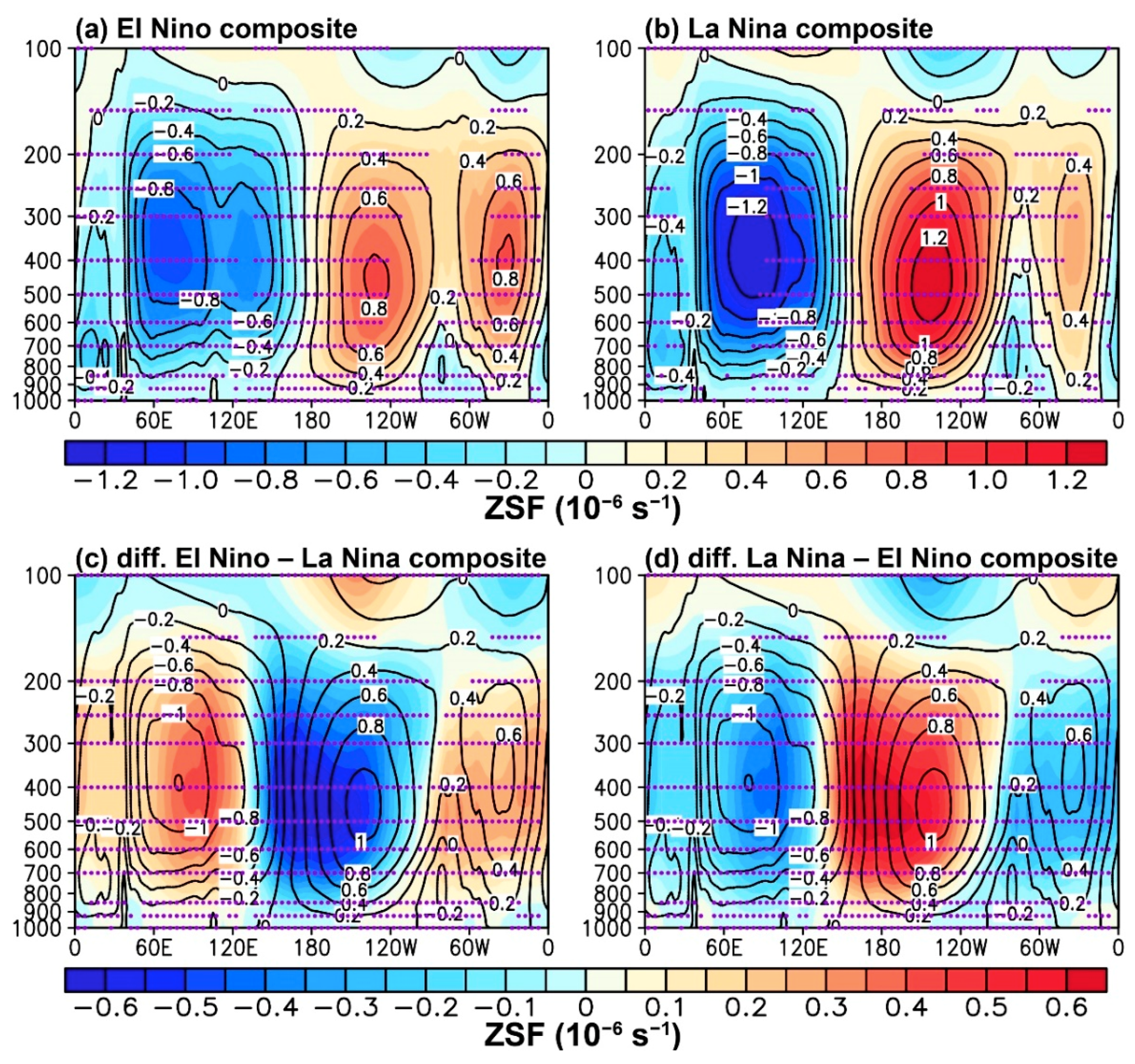
3.1. Response of the PWC to El Niño–Southern Oscillation (ENSO) Events

As mentioned previously, the meridional and zonal circulations can be effectively separated from the tropical atmospheric circulation (Figure 2), and the main characteristics of the PWC, IOC, and AOC can be well documented using the 3P-DGAC method (Figure 3); thus, the 3P-DGAC method is fairly appropriate for analyzing variations in the PWC. Furthermore, it is well known that the intensity of the PWC is closely related to ENSO events; thus, the 3P-DGAC-derived response of the PWC to ENSO events is first evaluated in this section.

Figure 4 displays the composites of the zonal circulations along the equator (5° S–5° N) for ENSO events based on the Oceanic Niño Index (ONI), which is defined as the three-month running mean of SST anomalies in the Niño 3.4 region (5° S–5° N, 120° W–170° W). These composites include all months with an ONI value larger than 0.5 K for El Niño events and with an ONI value less than −0.5 K for La Niña events. Figure 4 shows that the PWC becomes significantly weaker and shifts significantly eastward during El Niño events, and the opposite is approximately true during La Niña events, although the strength and width anomalies are asymmetric. In addition, accompanied by changes in the PWC, the IOC and AOC demonstrate significant changes during ENSO events, i.e., the IOC weakens (strengthens) during El Niño (La Niña) events, while the AOC strengthens (weakens) during El Niño (La Niña) events (Figure 4c,d).

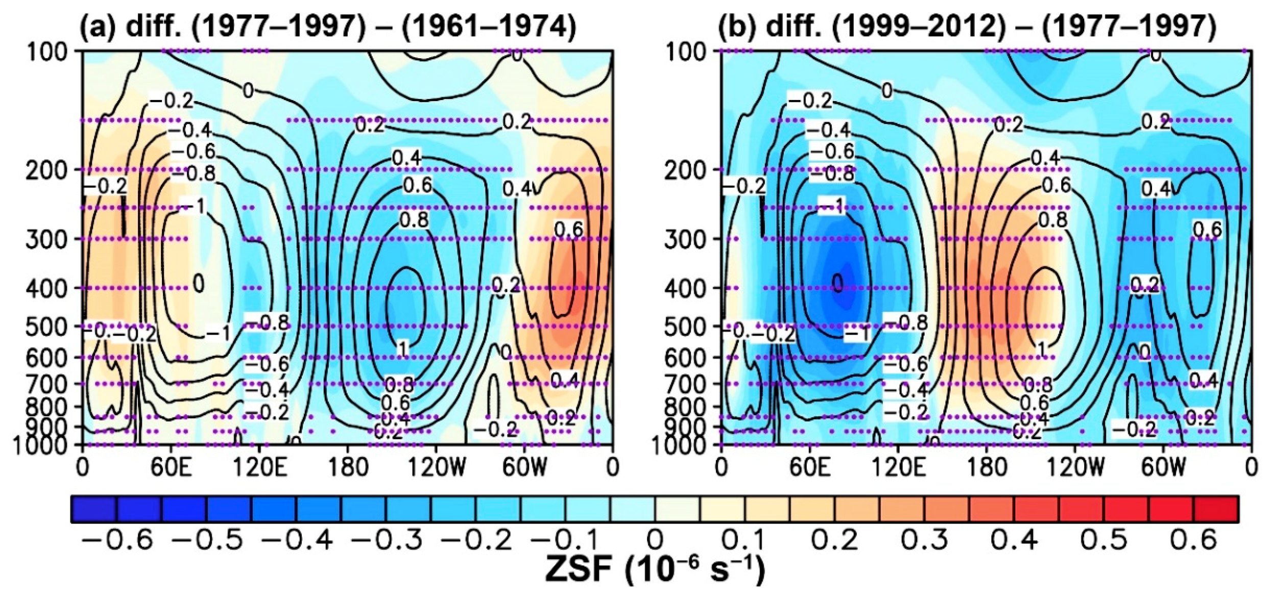
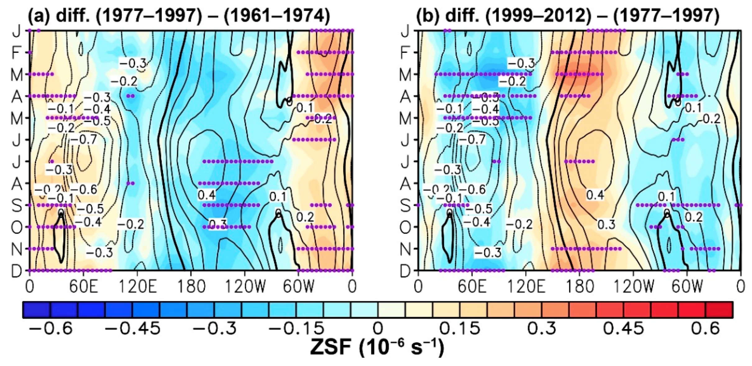
3.2. Interdecadal Variations of the PWC

As proposed previously, discrepancies in the changes in the PWC intensity among different studies may be caused by the different time periods selected in these studies. In addition, according to the changes in the SLP gradient between the eastern and western Pacific (Figure 1), obvious interdecadal variations of the SLP gradient can be observed during 1961–2012; thus, we separate the time period 1961–2012 into three parts, i.e., 1961–1974, 1977–1997, and 1999–2012.

Figure 5 displays the differences in the tropical zonal circulations between the time periods 1961–1974 and 1977–1997 and 1977–1997 and 1999–2012. Figure 5 shows that the PWC weakens and shifts eastward between 1961–1974 and 1977–1997 and strengthens and shifts westward between 1977–1997 and 1999–2012. Meanwhile, the IOC (AOC) weakens (strengthens) between the first pair of periods, while the IOC (AOC) strengthens (weakens) between the second pair of periods. In addition, because the PWC has an obvious seasonal cycle [7,39,40], this seasonality and its corresponding changes should be examined; thus, we further examine whether the zonal circulation changes shown in Figure 5 depend on the month. Figure 6 shows that the IOC, PWC, and AOC exhibit approximately identical changes, as shown in Figure 5, although there are minor changes in different months. For example, the greatest weakening trend of the PWC occurs in boreal autumn during the first pair of periods, while the largest strengthening trend appears in spring during the second pair of periods (Figure 6). Thus, the robust weakening (strengthening) and eastward (westward) shifting of the PWC between the first (second) pair of periods are not seasonally dependent. In general, the capability of the novel 3P-DGAC method to acquire interdecadal variations in the PWC has been confirmed.

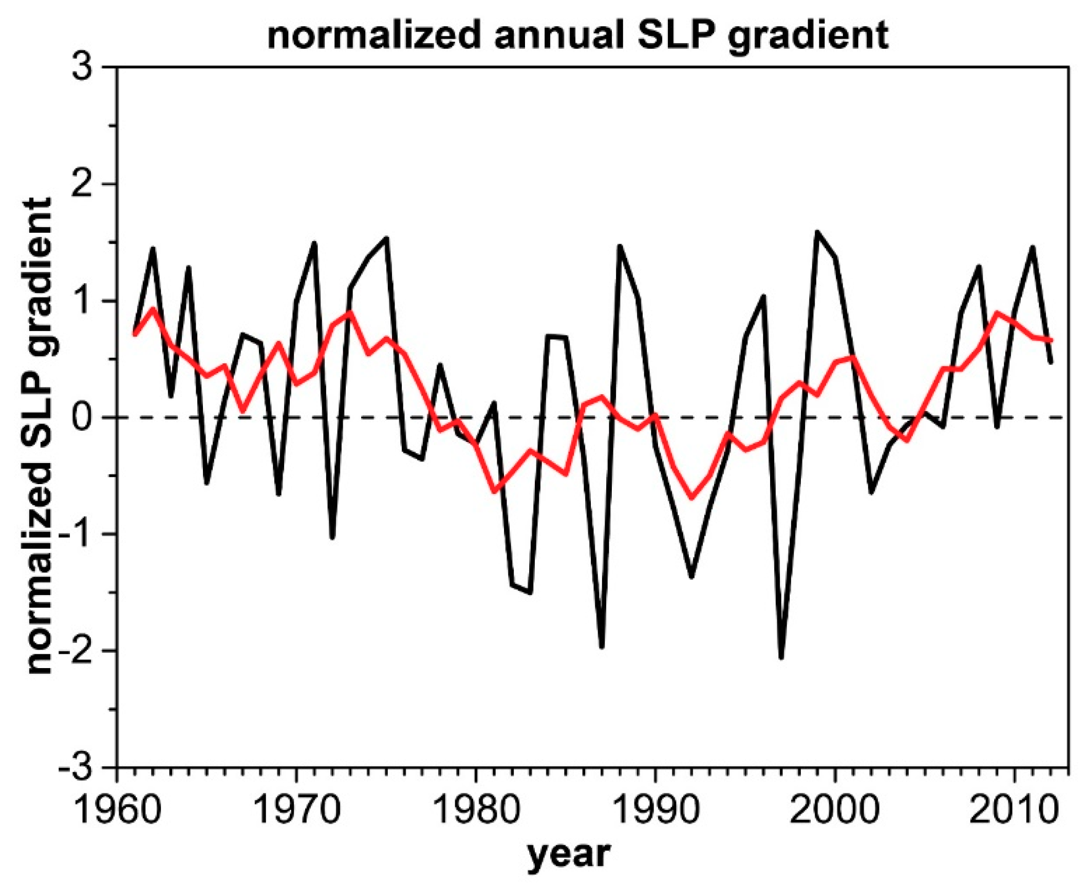
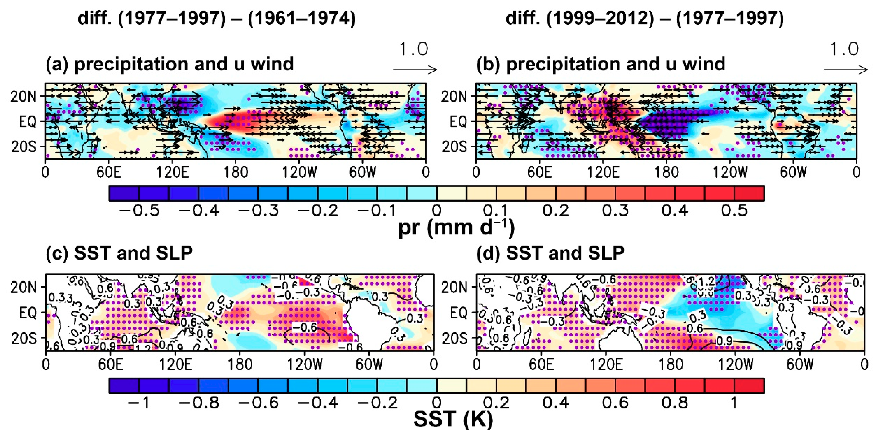
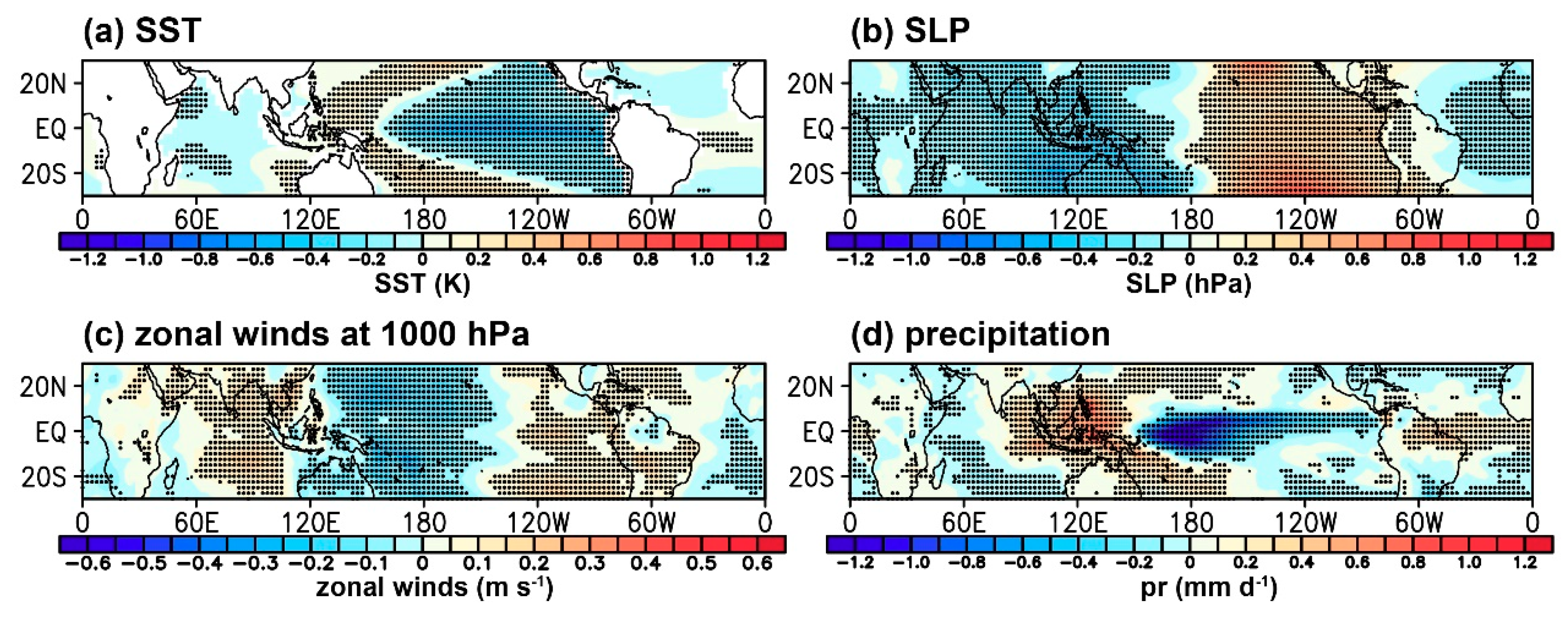
3.3. Interdecadal Variations of the Precipitation, Zonal Winds at 1000 hPa, SST, and SLP in the Low Latitudes

Along with changes in the PWC, the precipitation, zonal winds at 1000 hPa, SST, and SLP in the low latitudes have obvious interdecadal variations. Figure 7 shows that, from 1961–1974 to 1977–1997, the SST significantly increases (decreases) in the eastern (western) Pacific; thus, an abnormal SST gradient from the eastern to western Pacific forms. The changes in the SST result in a significantly weakened SLP gradient between the eastern and western Pacific (Figure 7c), which leads to significantly weakened easterly winds at 1000 hPa in the tropical Pacific regions and a consequently significantly weakened PWC (Figure 7a). The weakening of the PWC generates weakened rising (sinking) motions over the western (central and eastern) Pacific, leading to a significant decrease (increase) in precipitation over the western (central and eastern) Pacific (Figure 7a). Meanwhile, an abnormal SST gradient from the Indian Ocean to the western Pacific (from the eastern Pacific to the Atlantic) forms, which results in a significantly weakened (strengthened) SLP gradient and significantly weakened (strengthened) westerly (easterly) winds at 1000 hPa in the tropical Indian Ocean (Atlantic) regions. The weakening of the IOC generates weakened rising (sinking) motions over the eastern (western) Indian Ocean, leading to a significant decrease (increase) in precipitation over the eastern (western) Indian Ocean, while the strengthening of the AOC generates strengthened rising (sinking) motions over the western (eastern) Atlantic, leading to a significant increase (decrease) of precipitation over the western (eastern) Atlantic. From 1977–1997 to 1999–2012, the changes in the precipitation, zonal winds at 1000 hPa, SST, and SLP in the low latitudes are opposite to those between the first pair of periods (Figure 7b,d).

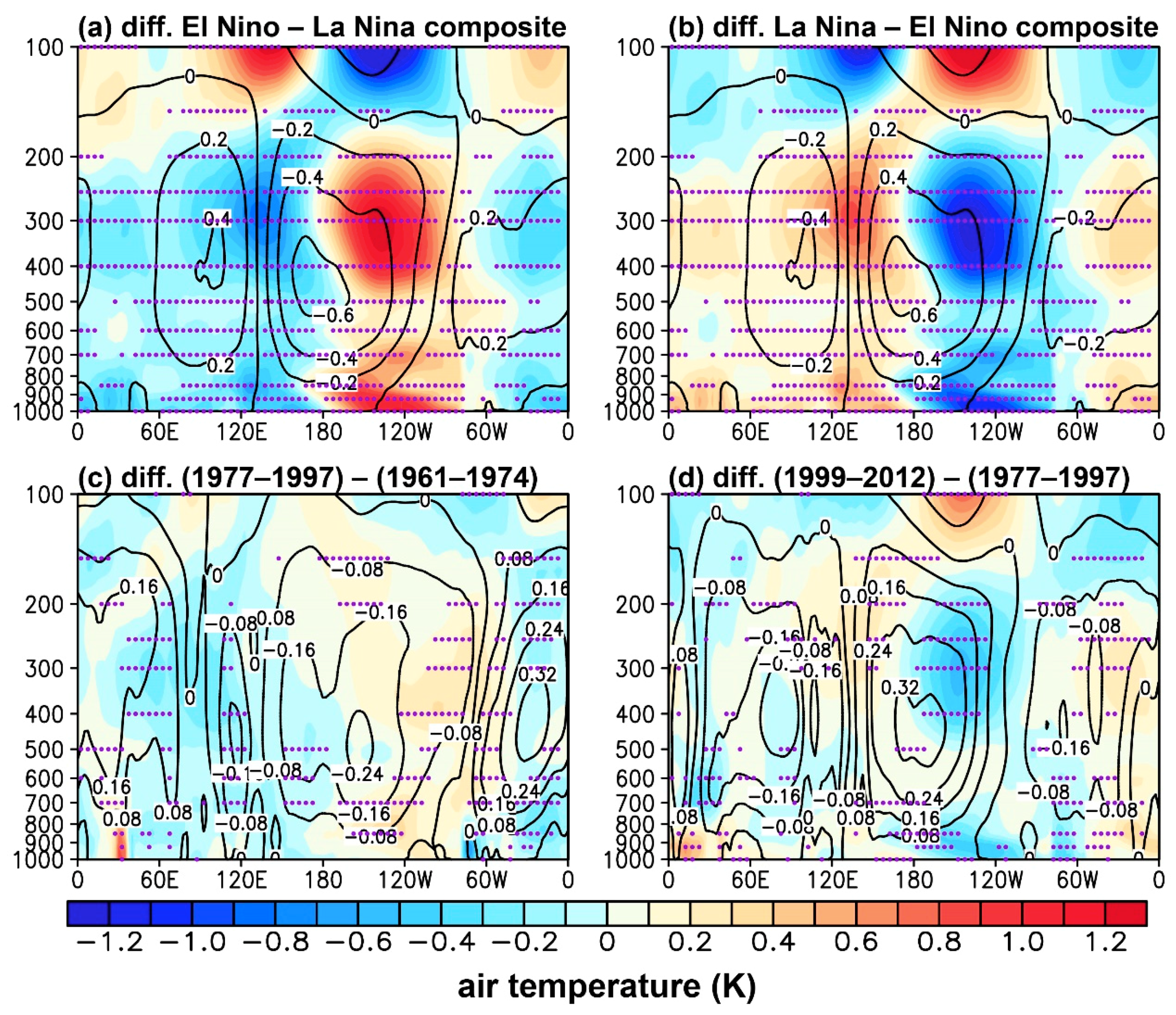
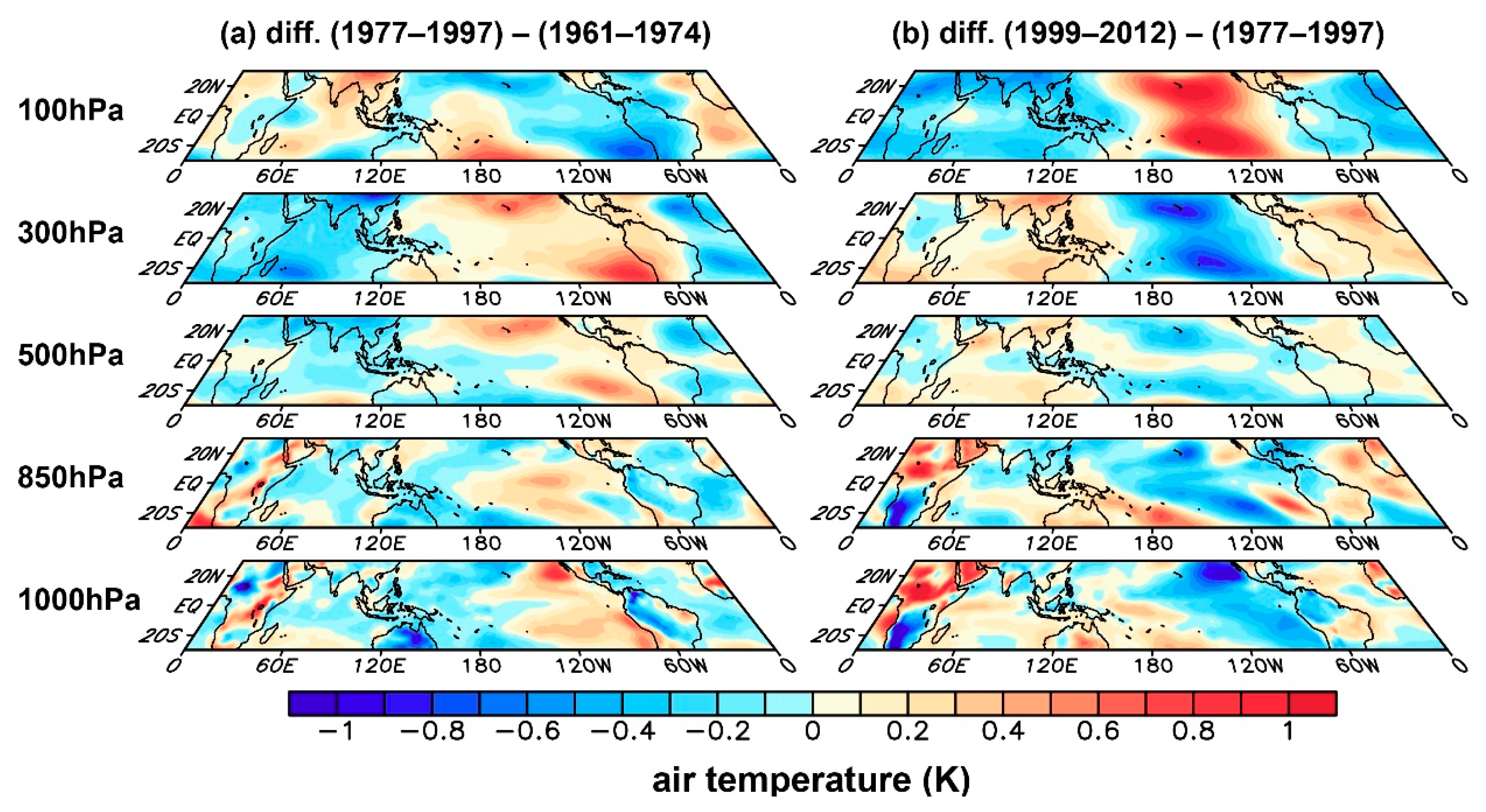
4. Connections between the Interdecadal Variations in the PWC Intensity and the Air Temperature Gradient Changes

The spatial pattern of the zonal circulation composites shown in Figure 4c,d is similar to the differences in the zonal circulations shown in Figure 5a,b. The spatial correlation coefficient is 0.7 between Figure 4c and Figure 5a and 0.89 between Figure 4d and Figure 5b. The similarities between the responses of the IOC, PWC, and AOC to ENSO events and the interdecadal variations in the three zonal circulations imply that they may have similar physical mechanisms. In addition, previous studies have suggested that changes in the air temperature gradient are critical to PWC variations [25,26,27]. For example, Bayr and Dommenget [27] noted that changes in the tropospheric temperature are more strongly correlated with changes in the SLP than changes in the SST. Thus, the connections between the interdecadal variations in the PWC intensity and the air temperature gradient changes (i.e., inhomogeneous air temperature changes) are investigated.

Figure 8 displays the differences in the zonal circulations (contours) and the inhomogeneous air temperature (shading) along the equator between ENSO events and between different time periods. It can be observed from Figure 8 that an inhomogeneous air temperature change is related to more rising where it is relatively warm and more sinking where it is relatively cold. Figure 8a,b shows that the composites of the zonal circulations related to ENSO coincide quite well with the inhomogeneous air temperature composites. This is apparent because abnormal rising motion occurs where the air temperature change is positive, and abnormal sinking occurs where the air temperature change is negative. Furthermore, Figure 8 shows that the inhomogeneous air temperature and zonal circulation composites between first (second) pair of periods are similar to those between El Niño and La Niña (La Niña and El Niño), although the magnitudes of the composites for different time periods (Figure 8c,d) are evidently smaller than those for ENSO events (Figure 8a,b).

Furthermore, Figure 9 displays 3D inhomogeneous air temperature differences between the periods 1961–1974 and 1977–1997 and between the periods 1977–1997 and 1999–2012 for the 1000, 850, 500, 300, and 100 hPa layers. For the composites of the inhomogeneous air temperature differences between the first pair of periods (Figure 9a), air temperature warming occurs from the low troposphere to middle–high troposphere (i.e., 1000–300 hPa) over the central and eastern Pacific regions. However, the differences in the inhomogeneous air temperature in the tropopause (i.e., 100 hPa) are opposite to those in the 1000–300 hPa pressure levels. The differences in the western Pacific are opposite to those in the central and eastern Pacific. Thus, these differences result in a secondary circulation with ascending movement in the warmer eastern Pacific regions, easterly movement in the upper troposphere, descending movement in the cooler western Pacific regions, and westerly movement in the lower troposphere. Because the direction of the secondary circulation, which is related to inhomogeneous air temperature changes, is contrary to the mean state of the PWC, the PWC should weaken between the first pair of periods. For the composites of the inhomogeneous air temperature differences between the second pair of periods (Figure 9b), the pattern is approximately the reverse of the corresponding pattern between the first pair of periods, namely, the inhomogeneous air temperature differences may lead to a secondary circulation with ascending movement in the western Pacific regions, westerly movement in the upper troposphere, descending movement in the eastern Pacific regions, and easterly movement in the lower troposphere. Thus, because the direction of the secondary circulation between the second pair of periods is the same as the mean state of the PWC, the PWC should strengthen. It is important to note that, for the second pair of periods, differences in the inhomogeneous air temperature over the tropical Atlantic and the eastern Pacific also result in a secondary circulation with ascending motion in the Atlantic and descending motion in the eastern Pacific, which amplify the intensification of the PWC [19]. Similarly, the warming of the Indian Ocean also contributes to the strengthening of the PWC, since warming can lead to abnormal rising motion in the warming pool region. In general, interdecadal variations in the PWC intensity are closely connected with air temperature gradient changes.

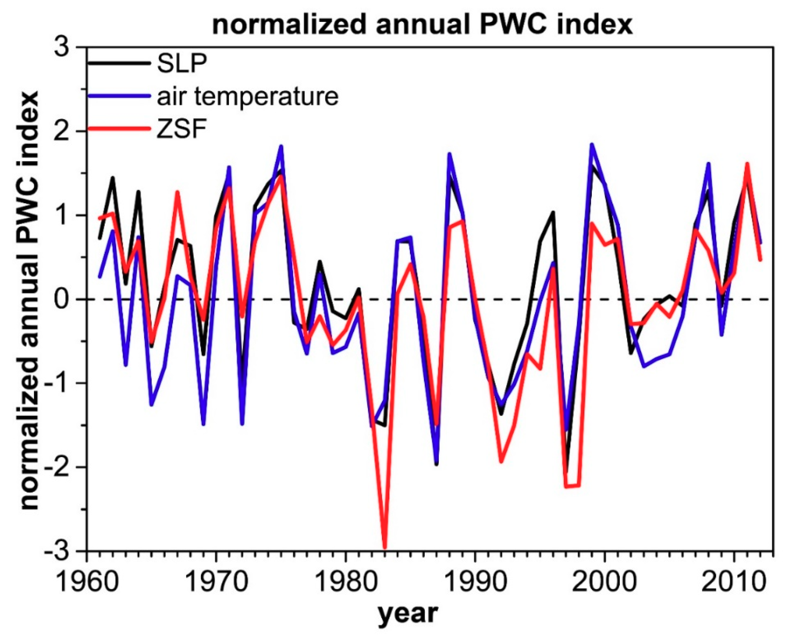
5. Novel Index for the PWC Intensity Based on Air Temperature

As proposed previously, interdecadal variations in the PWC intensity are closely connected with air temperature gradient changes; thus, a novel index for the PWC intensity based on air temperature has been defined as follows:

$${\mathrm{T}}_{\mathrm{index}}={\mathrm{TW}}_{1000\mathrm{hPa}}+{\mathrm{TW}}_{500\mathrm{hPa}}+{\mathrm{TE}}_{100\mathrm{hPa}}-\left({\mathrm{TE}}_{1000\mathrm{hPa}}+{\mathrm{TE}}_{500\mathrm{hPa}}+{\mathrm{TW}}_{100\mathrm{hPa}}\right)$$

(13)

where $\mathrm{T}$ is air temperature, $\mathrm{TW}$ represents the mean air temperature over the region (5° S–5° N, 80° W–160° W), $\mathrm{TE}$ is the mean air temperature over the region (5° S–5° N, 80° E–160° E), and the subscripts indicate different pressure levels.

To evaluate the capability of the novel index in representing the PWC intensity, the time series of the normalized annual mean tropical PWC intensity indices based on the SLP, air temperature, and ZSF are plotted (Figure 10). Figure 10 shows that the time series of these three indices are quite similar, and the correlation coefficient between the PWC intensity index based on the air temperature and the PWC intensity index based on the SLP (ZSF) is 0.93 (0.78). In addition, Figure 11 shows that when the ${\mathrm{T}}_{\mathrm{index}}$ is positive, an abnormal SST gradient from the western to eastern Pacific occurs, which results in a significantly strengthened SLP gradient between the eastern and western Pacific, significantly strengthened easterly winds at 1000 hPa in the tropical Pacific regions, and thus, a significantly strengthened PWC. The strengthening of the PWC generates strengthened rising (sinking) motions over the western (central and eastern) Pacific, leading to a significant increase (decrease) in precipitation over the western (central and eastern) Pacific. Thus, we conclude that changes in the PWC intensity can be well represented by using the novel index of the PWC intensity based on air temperature.

The novel index provides a new opportunity for the prediction of the PWC by using dynamical equations derived from the 3P-DGAC method [26]. Furthermore, Hu et al. [26] proposed that inhomogeneous air temperature change can lead not only to changes in the PWC, but also to changes in the baroclinicity of the horizontal circulation. In other words, the influences of inhomogeneous air temperature changes on changes in the PWC and the baroclinicity of the horizontal circulation can be effectively separated using the 3P-DGAC method; thus, the influence of inhomogeneous air temperature changes on changes in the PWC can be more correctly described. In future studies, we will quantitatively investigate the influences of the inhomogeneous air temperature gradient on changes in the PWC.

6. Summary

Recently, to obtain a unified description of atmospheric circulation from a global perspective, a novel 3P-DGAC method was proposed. In this study, we aim to determine whether the novel 3P-DGAC method can acquire the interdecadal variations in the PWC during 1961–2012 and the connection of these variations to inhomogeneous air temperature changes.

Our results show that the PWC with ascending motion over the western Pacific and descending motion over the eastern Pacific can be generally represented by using the ZSF derived from the 3P-DGAC method. Furthermore, we analyze interdecadal changes in the PWC during three time periods, i.e., 1961–1974, 1979–1997, and 1999–2012, using the 3P-DGAC method. The PWC weakens in the first pair of time periods and strengthens in the second pair, corresponding to the climate shift in approximately 1976/77 [41,42] and recent interdecadal changes since the late 1990s [42,43,44,45]. With changes in the PWC, the precipitation, SLP, SST, and zonal winds at 1000 hPa also exhibit evident interdecadal changes. Therefore, we conclude that the interdecadal variations in the PWC over 1961–2012 can be well documented by the 3P-DGAC method.

In the above analysis, we find that the three main tropical zonal circulations are coupled with each other. Specifically, similar to the PWC, two other zonal circulations, i.e., the IOC in the Indian Ocean and the AOC in the Atlantic, also have interdecadal changes. In the first (second) pair of periods, the IOC generally weakens (strengthens), and the AOC generally strengthens (weakens).

We further investigate the changes in inhomogeneous air temperature from the low troposphere to the tropopause, and conclude that the interdecadal variations in the PWC intensity are closely connected with the air temperature gradient changes. Furthermore, a novel index for the PWC intensity based on air temperature is defined, and the capability of the novel index in representing the PWC intensity is evaluated. The novel index provides a new opportunity for PWC predictions by using dynamical equations derived from the 3P-DGAC method [26]. However, we cannot confirm that the interdecadal variations in the PWC intensity are caused by the changes in inhomogeneous air temperature although they are closely related, and much more efforts are needed in order to study the relationship between the two, since SST, convection, tropospheric temperature, and atmospheric circulations are coupled in the system.

It should be mentioned that by using the mass stream function (MSF; the definition of MSF is presented in the Supplementary Materials) derived from the method proposed by Schwendike et al. [40,46] (a brief introduction of the method is provided in the Supplementary Materials), the interdecadal variations in the PWC and its connection to inhomogeneous air temperature changes can also be obtained (Figures S3–S7). It can be observed that Figures S3–S5 are similar to Figure 5, Figure 6 and Figure 8, although the differences in the PWC between the periods 1961–1974 and 1977–1997 shown in Figure 8c match better with the inhomogeneous air temperature changes than those shown in Figure S5c. In addition, Figure S6 shows that the time series of the PWC intensity based on the SLP, air temperature, and MSF are quite similar, and the correlation coefficient between the PWC intensity index based on the MSF and the PWC intensity index based on the SLP (air temperature) is 0.68 (0.56), which is smaller than the correlation coefficient between the PWC intensity index based on the ZSF and the PWC intensity index based on the SLP (0.86) and that based on air temperature (0.79). Although the results based on the ZSF display better performance in representing the changes in PWC than those based on the MSF in this paper, we cannot conclude that the 3P-DGAC method is better than the method proposed by Schwendike et al. [40,46] in representing the PWC, and much more investigation are needed in order to study the difference and similarity between the two methods.

Compared with the MSF and the SLP contrast, there are advantages of the ZSF (or the 3P-DGAC method) in the investigation of the PWC because the ZSF can be directly predicted, and theoretical experiments can be conducted by using the dynamical equations derived from the 3P-DGAC method [26]. It can be observed from the Supplementary Materials (see also in Hu et al. [26]) that the new dynamical equations of the horizontal, meridional, and zonal circulations (Equations (S10)–(S13)) can be obtained by combining the 3P-DGAC method and the primary equations. Equations (S10)–(S13) can be used to diagnose and predict the variations of the horizontal, meridional, and zonal circulations directly from the perspective of stream functions instead of the velocity field. Namely, by using Equations (S10)–(S13), the PWC (i.e., zonal circulation) can be directly predicated ($W$ is the stream function of zonal circulation and $W$ is the ZSF in this paper). Thus, the 3P-DGAC method may be potentially useful and advantageous for the study of the PWC. The investigation of the PWC by using the new dynamical equations is beyond the scope of this study and needs to be further investigated.

It can be observed from Equation (S11) that the inhomogeneous air temperature changes in the zonal direction are connected with changes related to the horizontal, meridional, and zonal circulations. In addition, the Equation (S15), which is the simplified equation of Equation (S11), shows that the inhomogeneous air temperature change is mainly related to the changes of the PWC and the baroclinicity of the horizontal circulation. This may be why the correlation coefficient between the PWC intensity index based on the air temperature and the PWC intensity index based on the ZSF (SLP) is high. Notably, it can be seen from Equation (S15) that the inhomogeneous air temperature gradient is related not only to changes in the PWC, but also to changes in the baroclinicity of the horizontal circulation, and the quantitative relationship between the inhomogeneous air temperature gradient and the PWC and baroclinicity will be investigated in the future. The dynamical Equations (S10)–(S13) and the simplified dynamical Equations (S14)–(S17) are potentially important to our understanding of the relationship between changes in the PWC strength and changes in the tropospheric air temperature gradient, which may be helpful for the prediction of the PWC. Much more efforts are needed in the future.

References

1. Bjerknes, J. Atmospheric teleconnections from the equatorial Pacific. Mon. Weather Rev. 1969, 97, 163–172. [Google Scholar] [CrossRef]
2. Philander, S.G.H. El Niño, La Niña, and the Southern Oscillation; Academic Press: San Diego, CA, USA, 1990. [Google Scholar]
3. Power, S.; Casey, T.; Folland, C.; Colman, A.; Mehta, V. Inter-decadal modulation of the impact of ENSO on Australia. Clim. Dyn. 1999, 15, 319–324. [Google Scholar] [CrossRef]
4. Kosaka, Y.; Xie, S.-P. Recent global-warming hiatus tied to equatorial Pacific surface cooling. Nature 2013, 501, 403–407. [Google Scholar] [CrossRef] [PubMed] [Green Version]
5. England, M.H.; Mcgregor, S.; Spence, P.; Meehl, G.A.; Timmermann, A.; Cai, W.; Gupta, A.S.; McPhaden, M.J.; Purich, A.; Santoso, A. Recent intensification of wind-driven circulation in the Pacific and the ongoing warming hiatus. Nat. Clim. Chang. 2014, 4, 222–227. [Google Scholar] [CrossRef] [Green Version]
6. Ma, S.; Zhou, T. Changes of the tropical Pacific Walker circulation simulated by two versions of FGOALS model. Sci. China Earth Sci. 2014, 57, 2165–2180. [Google Scholar] [CrossRef]
7. Ma, S.; Zhou, T. Robust strengthening and westward shift of the tropical Pacific Walker circulation during 1979–2012: A comparison of 7 sets of reanalysis data and 26 CMIP5 dodels. J. Clim. 2016, 29, 3097–3118. [Google Scholar] [CrossRef]
8. Vecchi, G.A.; Soden, B.J.; Wittenberg, A.T.; Held, I.M.; Leetmaa, A.; Harrison, M.J. Weakening of tropical Pacific atmospheric circulation due to anthropogenic forcing. Nature 2006, 441, 73–76. [Google Scholar] [CrossRef] [PubMed]
9. Vecchi, G.A.; Soden, B.J. Global warming and the weakening of the tropical circulation. J. Clim. 2007, 20, 4316–4340. [Google Scholar] [CrossRef]
10. DiNezio, P.N.; Clement, A.C.; Vecchi, G.A.; Soden, B.J.; Kirtman, B.P.; Lee, S.K. Climate response of the equatorial Pacific to global warming. J. Clim. 2009, 22, 4873–4892. [Google Scholar] [CrossRef]
11. Yu, B.; Zwiers, F.W. Changes in equatorial atmospheric zonal circulations in recent decades. Geophys. Res. Lett. 2010, 37, L05701. [Google Scholar] [CrossRef]
12. Power, S.B.; Kociuba, G. What caused the observed twentieth-century weakening of the Walker circulation? J. Clim. 2011, 24, 6501–6514. [Google Scholar] [CrossRef]
13. Tokinaga, H.; Xie, S.-P.; Deser, C.; Yu, K.; Okumura, Y.M. Slowdown of the Walker circulation driven by tropical Indo-Pacific warming. Nature 2012, 491, 439–443. [Google Scholar] [CrossRef] [PubMed]
14. DiNezio, P.N.; Vecchi, G.A.; Clement, A.C. Detectability of changes in the Walker circulation in response to global warming. J. Clim. 2013, 26, 4038–4048. [Google Scholar] [CrossRef]
15. Kociuba, G.; Power, S.B. Inability of CMIP5 models to simulate recent strengthening of the Walker circulation: Implications for projections. J. Clim. 2015, 28, 20–35. [Google Scholar] [CrossRef]
16. Meng, Q.; Latif, M.; Park, W.; Keenlyside, N.S.; Semenov, V.A.; Martin, T. Twentieth century Walker circulation change: Data analysis and model experiments. Clim. Dyn. 2012, 38, 1757–1773. [Google Scholar] [CrossRef]
17. L’Heureux, M.L.; Lee, S.; Lyon, B. Recent multidecadal strengthening of the Walker circulation across the tropical Pacific. Nat. Clim. Chang. 2013, 3, 571–576. [Google Scholar] [CrossRef]
18. Sohn, B.J.; Yeh, S.W.; Schmetz, J.; Song, H.J. Observational evidences of Walker circulation change over the last 30 years contrasting with GCM results. Clim. Dyn. 2013, 40, 1721–1732. [Google Scholar] [CrossRef]
19. McGregor, S.; Timmermann, A.; Stuecker, M.F.; England, M.H.; Merrifield, M.; Jin, F.-F.; Chikamoto, Y. Recent Walker circulation strengthening and Pacific cooling amplified by Atlantic warming. Nat. Clim. Chang. 2014, 4, 888–892. [Google Scholar] [CrossRef] [Green Version]
20. Sandeep, S.; Stordal, F.; Sardeshmukh, P.D.; Compo, G.P. Pacific Walker circulation variability in coupled and uncoupled climate models. Clim. Dyn. 2014, 43, 103–117. [Google Scholar] [CrossRef]
21. Dong, B.; Lu, R. Interdecadal enhancement of the Walker circulation over the tropical Pacific in the late 1990s. Adv. Atmos. Sci. 2013, 30, 247–262. [Google Scholar] [CrossRef]
22. Allan, R.; Ansell, T. A New Globally complete monthly historical gridded mean sea level pressure dataset (HadSLP2): 1850–2004. J. Clim. 2006, 19, 5816–5842. [Google Scholar] [CrossRef]
23. Deser, C.; Wallace, J.M. Large-scale atmospheric circulation features of warm and cold episodes in the tropical Pacific. J. Clim. 1990, 3, 1254–1281. [Google Scholar] [CrossRef]
24. Garcia, S.R.; Kayano, M.T. Climatological aspects of Hadley, Walker and monsoon circulations in two phases of the Pacific decadal oscillation. Theor. Appl. Climatol. 2008, 91, 117–127. [Google Scholar] [CrossRef]
25. Bayr, T.; Dommenget, D.; Martin, T.; Power, S.B. The eastward shift of the Walker circulation in response to global warming and its relationship to ENSO variability. Clim. Dyn. 2014, 43, 2747–2763. [Google Scholar] [CrossRef]
26. Hu, S.; Cheng, J.; Xu, M.; Chou, J. Three-pattern decomposition of global atmospheric circulation: Part II—Dynamical equations of horizontal, meridional and zonal circulations. Clim. Dyn. 2018, 50, 2673–2686. [Google Scholar] [CrossRef]
27. Bayr, T.; Dommenget, D. The tropospheric land-sea warming contrast as the driver of tropical sea level pressure changes. J. Clim. 2013, 26, 1387–1402. [Google Scholar] [CrossRef]
28. Xu, M. Study on the Three Dimensional Decomposition of Large Scale Circulation and Its Dynamical Feature. Ph.D. Thesis, Lanzhou University, Lanzhou, China, May 2001. (In Chinese). [Google Scholar]
29. Hu, S. The Three-Dimensional Expansion of Global Atmospheric Circumfluence and Characteristic Analyze of Atmospheric Vertical Motion. Ph.D. Thesis, Lanzhou University, Lanzhou, China, June 2006. (In Chinese). [Google Scholar]
30. Liu, H.; Hu, S.; Xu, M.; Chou, J. Three-dimensional decomposition method of global atmospheric circulation. Sci. China Ser. D 2008, 51, 386–402. [Google Scholar] [CrossRef]
31. Hu, S.; Cheng, J.; Chou, J. Novel three-pattern decomposition of global atmospheric circulation: Generalization of traditional two-dimensional decomposition. Clim. Dyn. 2017, 49, 3573–3586. [Google Scholar] [CrossRef]
32. Hu, S.; Chou, J.; Cheng, J. Three-pattern decomposition of global atmospheric circulation: Part I—Decomposition model and theorems. Clim. Dyn. 2018, 50, 2355–2368. [Google Scholar] [CrossRef]
33. Cheng, J.; Gao, C.; Hu, S.; Feng, G. High-stability algorithm for the three-pattern decomposition of global atmospheric circulation. Theor. Appl. Climatol. 2018, 133, 851–866. [Google Scholar] [CrossRef]
34. Cheng, J.; Xu, Z.; Hu, P.; Hou, X.; Gao, C.; Hu, S.; Feng, G. Significant role of orography in shaping the northern Hadley circulation and its poleward expansion during boreal summer. Geophys. Res. Lett. 2018, 45, 6619–6627. [Google Scholar] [CrossRef]
35. Ebita, A.; Kobayashi, S.; Ota, Y.; Moriya, M.; Kumabe, R.; Onogi, K.; Harada, Y.; Yasui, S.; Miyaoka, K.; Takahashi, K.; et al. The Japanese 55-year reanalysis “JRA-55”: An interim report. SOLA 2011, 7, 149–152. [Google Scholar] [CrossRef]
36. Chen, M.; Xie, P.; Janowiak, J.E.; Arkin, P.A. Global land precipitation: A 50-y monthly analysis based on gauge observations. J. Hydrometeorol. 2002, 3, 249–266. [Google Scholar] [CrossRef]
37. Huang, B.; Thorne, P.W.; Banzon, V.F.; Boyer, T.; Chepurin, G.; Lawrimore, J.H.; Menne, M.J.; Smith, T.M.; Vose, R.S.; Zhang, H.M. NOAA Extended Reconstructed Sea Surface Temperature (ERSST); Version 5; NOAA National Centers for Environmental Information: Asheville, NC, USA, 2017. [Google Scholar] [CrossRef]
38. Holton, J.R. Synoptic-scale motions I: Quasi-geostrophic analysis. In An Introduction to Dynamic Meteorology, 4th ed.; Cynar, F., Ed.; Elsevier Academic Press: Amsterdam, The Netherlands, 2004; pp. 139–176. [Google Scholar]
39. Yu, B.; Zwiers, F.W.; Boer, G.J.; Ting, M.F. Structure and variances of equatorial zonal circulation in a multimodel ensemble. Clim. Dyn. 2012, 39, 2403–2419. [Google Scholar] [CrossRef]
40. Schwendike, J.; Govekar, P.; Reeder, M.J.; Wardle, R.; Berry, G.J.; Jakob, C. Local partitioning of the overturning circulation in the tropics and the connection to the Hadley and Walker circulations. J. Geophys. Res. Atmos. 2014, 119, 1322–1339. [Google Scholar] [CrossRef] [Green Version]
41. Graham, N.E. Decadal-scale climate variability in the tropical and North Pacific during the 1970s and 1980s: Observations and model results. Clim. Dyn. 1994, 10, 135–162. [Google Scholar] [CrossRef]
42. Burgman, R.J.; Clement, A.C.; Mitas, C.M.; Chen, J.; Esslinger, K. Evidence for atmospheric variability over the Pacific on decadal timescales. Geophys. Res. Lett. 2008, 35, L01704. [Google Scholar] [CrossRef]
43. Chen, J.; DelGenio, A.D.; Carlson, B.E.; Bosilovich, M.G. The spatiotemporal structure of twentieth-century climate variations in observations and reanalysis. Part II: Pacific pan-decadal variability. J. Clim. 2008, 21, 2634–2650. [Google Scholar] [CrossRef]
44. Wang, H.; Mehta, V.M. Decadal variability of the Indo-Pacific warm pool and its association with atmospheric and oceanic variability in the NCEP-NCAR and SODA reanalyses. J. Clim. 2008, 21, 5545–5565. [Google Scholar] [CrossRef]
45. Zhang, L.; Wu, L.; Yu, L. Oceanic origin of a recent La Niña-like trend in the tropical Pacific. Adv. Atmos. Sci. 2011, 28, 1109–1117. [Google Scholar] [CrossRef]
46. Schwendike, J.; Berry, G.J.; Reeder, M.J.; Jakob, C.; Govekar, P.; Wardle, R. Trends in the local Hadley and local Walker circulations. J. Geophys. Res. 2015, 120, 7599–7618. [Google Scholar] [CrossRef] [Green Version]
Figure 1. Time series of the normalized annual mean sea level pressure (SLP) gradient over the tropical Pacific (black line), defined as the mean SLP over the region (5° S–5° N, 80° W–160° W) minus the mean SLP over the region (5° S–5° N, 80° E–160° E) derived from the HadSLPr dataset [22] for 1961–2012. The red line represents the 5-year running mean of the SLP gradient.
Atmosphere 09 00469 g001
Figure 2. Mean state (1961–2012) of the annual mean (a) vertical velocity, (b) vertical velocity of the meridional circulation, and (c) vertical velocity of the zonal circulation at 500 hPa using the JRA-55 reanalysis dataset [35]. The vertical velocities have been multiplied by −1, and positive (negative) values represent rising (sinking) motion. The unit for vertical velocity is Pa s−1.
Atmosphere 09 00469 g002
Figure 3. (a) Mean state (1961–2012) of the annual mean meridionally-averaged zonal stream function (ZSF) (10−6 s−1) between 5° S and 5° N using the JRA-55 reanalysis dataset [35]. (b) Inhomogeneous part of (a) ((a) minus the global zonal mean of (a)).
Atmosphere 09 00469 g003
Figure 4. Composite of the zonal circulations along the equator (5° S–5° N) in JRA-55 reanalysis dataset [35] for (a) El Niño and (b) La Niña based on the ONI (5° S–5° N, 120° W–170° W). (c) Contours: mean state (1961–2012) of the zonal circulations; shading: difference between El Niño–La Niña; (d) same as (c) but for the mean state of the zonal circulations (contours) and difference between La Niña–El Niño (shading). The composites which are statistically significant at the 5% confidence level are dotted in purple. Diff.: means minus in math.
Atmosphere 09 00469 g004
Figure 5. Contours in (a) and (b): mean state (1961–2012) of the annual mean zonal circulations along the equator (5° S–5° N); shading: differences in the annual mean zonal circulations between (a) the periods 1961–1974 and 1977–1997 and (b) the periods 1977–1997 and 1999–2012. The changes statistically significant at the 5% confidence level are dotted in purple.
Atmosphere 09 00469 g005
Figure 6. Contours in (a) and (b): mean state (1961–2012) of the monthly mean of vertically averaged zonal circulations along the equator (5° S–5° N); shading: differences in the monthly mean of vertically averaged zonal circulations between (a) the periods 1961–1974 and 1977–1997 and (b) the periods 1977–1997 and 1999–2012. The composites which are statistically significant at the 5% confidence level are dotted in purple.
Atmosphere 09 00469 g006
Figure 7. Differences in the precipitation (shading in (a); mm d−1), zonal winds of zonal circulation at 1000 hPa (vectors in (a); m s−1), sea surface temperature (SST) (shading in (c); K), and SLP (contours in (c); hPa) at low latitudes (30° S–30° N) between the periods 1961–1974 and 1977–1997. (b,d) are the same as (a,c) but show the differences between the periods 1977–1997 and 1999–2012. The vectors (contours) are plotted only for regions with zonal wind (SLP) changes that are statistically significant at the 5% confidence level. The changes in precipitation and SST that are statistically significant at the 5% confidence level are dotted in purple. The black solid (dashed) lines represent the positive (negative) changes in the SLP. The arrows shown in the top right corner of (a) and (b) are the reference vectors.
Atmosphere 09 00469 g007
Figure 8. Differences in the zonal circulation (contours; 10−6 s−1) and inhomogeneous air temperature (shading; K) along the equator (5° S–5° N) between (a) El Niño and La Niña, (b) La Niña and El Niño, (c) the periods 1961–1974 and 1977–1997, and (d) the periods 1977–1997 and 1999–2012. The composites of zonal circulation and inhomogeneous air temperature which are both statistically significant at the 5% confidence level are dotted in purple.
Atmosphere 09 00469 g008
Figure 9. Differences in the inhomogeneous air temperature (K) at low latitudes (30° S–30° N) between (a) the periods 1961–1974 and 1977–1997 and (b) the periods 1977–1997 and 1999–2012 for layers 1000, 850, 500, 300, and 100 hPa.
Atmosphere 09 00469 g009
Figure 10. Time series (1961–2012) of the normalized annual mean tropical Pacific Walker circulation (PWC) intensity indices based on the SLP (defined as the mean SLP over the region (5° S–5° N, 80° W–160° W) minus the mean SLP over the region (5° S–5° N, 80° E–160° E); black line), air temperature (defined as in Equation (13); blue line), and ZSF (defined as the mean value of the inhomogeneous ZSF over the region (5° S–5° N, 120° W–160° W, 300–600 hPa); red line).
Atmosphere 09 00469 g010
Figure 11. Spatial pattern of the regressed (a) SST (K), (b) SLP (hPa), (c) zonal winds of the zonal circulation at 1000 hPa (m s−1), and (d) precipitation (mm d−1) against the normalized PWC intensity index based on the air temperature for the period 1961–2012. The regression coefficients statistically significant at the 5% confidence level are dotted in black.
Atmosphere 09 00469 g011