Long-Term Wintertime Trend of Zonally Asymmetric Ozone in Boreal Extratropics During 1979–2016

Abstract

Strong zonally asymmetric ozone (ZAO) changes are observed in the boreal extratropics for winter. During the TOMS (Total Ozone Mapping Spectrometer) period (1979–1992) the decrease of zonally asymmetric total ozone (ZATO) was twice as large as the observed zonal mean total ozone trend over Europe in January mainly caused by ultra-long wave transport. Recent studies have demonstrated that the ozone evolution reveals three different quasi-bidecadal trend stages: (i) Decline, (ii) leveling, and (ii) healing. This study focuses on the ZAO structure in boreal extratropics and on ozone transport changes by ultra-long waves during winter months. ERA-Interim data together with a linearized transport model are used. During the healing stage ZATO increases significantly over the North Atlantic/European region for January. The ZATO increase (healing stage) and ZATO decrease (decline stage) are caused by different monthly mean ozone transport characteristics of ultra-long planetary waves over the North Atlantic/European region. Furthermore, the vertical advection (ageostrophic transport) of ozone versus its horizontal component dominates in the lower and middle stratosphere during the healing stage. It is hypothesized that these ageostrophic wind changes are mainly caused by a wave train directed northeastwards which seems to be directly linked to the Arctic warming.

1. Introduction

Ozone in the atmosphere gains its importance due to its absorption of harmful ultraviolet radiation and its action as an effective absorber of terrestrial longwave radiation in the atmosphere. A strong decrease of ozone has been observed since the late 1970s referred to as ozone hole in the Southern Hemisphere, requiring a recovery of ozone by humankind. Due to the Montreal Protocol (1987, Montreal Protocol on substances that deplete the ozone layer) anthropogenic emissions of ozone depleting substances (ODS), such as chlorofluorocarbon and halons are reduced, yielding a decline of the ODS in the stratosphere. However, greenhouse gases like CO₂, N₂O, and CH₄ are still increasing.

The complex interaction between chemistry and transport of minor constituents in its action on trends is not fully understood including the global warming effects [1,2,3,4]. The expectation is the recovery of ozone in the stratosphere in this century. The recovery involves fingerprints or multiple stages [5,6]; (i) A strong decline (decline stage); (ii) a leveling off of the depletion (leveling stage); and (iii) an identifiable ozone increase (healing stage). This can be followed by a possible stage of super-recovery, in which ozone concentration increases faster than ODS decline. In the literature, it is expected that ozone will heal or recover in mid to end of this century [2,4,7].

Note that the zonally dependent or zonally asymmetric ozone (ZAO) is defined as the deviation from the zonal mean ozone [8]. There are two pathways how zonally asymmetric ozone influences the extratropical circulation [9]. The first pathway includes a modulation of propagation and damping of planetary waves by ZAO due to radiative processes. The second pathway includes a modulation of the wave-ozone flux convergence by the ozone wave. In a steady state both pathways are important to change the zonal mean circulation.

Due to its radiative forcing, the zonally asymmetric ozone has an influence on the atmospheric circulation [10] of the Northern [11,12] and Southern Hemisphere [13,14,15,16,17]. The consideration of zonally asymmetric ozone influences the zonal mean ozone transport (e.g., [18]) or the photochemical destabilization of free Rossby waves (e.g., [19]), and the planetary wave drag [20]. Taking the zonally asymmetric ozone into account, it will change the wave propagation and damping, which results in a change of the upward propagation of planetary waves into the stratosphere, where their divergence of the Eliassen-Palm flux changes the mean circulation again [21].

Both, the zonal mean and the zonally asymmetric component of ozone, reveal a linear trend and multidecadal oscillations, including the healing stage. Both groups, hood and Zaff (1995) [22] and Peters et al. (1996) [23], Peters and Entzian (1996, 1999) [24,25], show independently that decadal changes of ZAO are correlated with decadal changes of geopotential ultra-long waves. This indicates that the trend pattern of the ultra-long waves mainly determines the trend pattern of ZAO for each winter month, especially in January over Europe where the zonally asymmetric change is comparable to the zonal mean ozone trend of about 20 DU until the end of the last century [26]. Recently, Zhang et al. (2018) [27] studied trends in zonally asymmetric ozone and geopotential height disturbances (deviations from zonal mean) of the Northern Hemisphere for mean winter conditions. In satellite-based observations (ERA-Interim [28], MERRA [29]; 1979–2015) Zhang et al. [27] found regional significant mean winter trends in ZAO, and confirmed the relative small contribution of chemical processes to ZATO trends with the help of model runs of a chemistry-climate model and an offline chemical transport model. This supports the usage of a linear ozone transport model without any chemistry as already used by Hood and Zaff [22] and Peters and Entzian [24]. The linear transport model results demonstrate the main role of planetary waves in ozone transport and their changes for the extratropics. Furthermore, Zhang et al. [27] identified with the three leading Empiral Orthogonal Functions the three surface patterns (Arctic Oscillation index, Cold Ocean-Warm Land index, North Pacific index) which mainly modulate the changes of geopotential height in the stratosphere in winter means during the 1979–2015 period.

However, for the healing stage a study of ZAO changes in the extratropics of the Northern Hemisphere for each winter month is still open. Peters and Entzian [24] discussed the monthly mean trend of ZATO and found strong differences between December, January, and February during the TOMS period. The structure changes of zonally asymmetric ozone for and between ozone stages during different winter months, and the understanding of transport characteristics of ultra-long planetary wave during each winter month are still unclear.

This study focuses on the zonally asymmetric ozone structure in boreal extratropics and on ozone transport changes by ultra-long waves during the winter months of the last four decades. ERA-Interim data are used for diagnosis. A simple linearized transport model is applied in order to examine different wave transport characteristics of ozone. The study is an extension of the investigation of [25] into the healing stage. The focus lies on secular trends of 15-year intervals (quasi-bidecadal) for each winter month (DJF) in order to compare secular trends between all three stages.

The paper is organized in the following way. In Section 2 the methodology and data set are described. Quasi-bidecadal trends for ZAO and geopotential disturbances of ERA-Interim for the winter month of January are presented in Section 3, for December and February in the Figures S2c and S3c; supplemental material. Furthermore, results of a simple linear transport model calculation of ZAO are shown in order to examine transport characteristics of ultra-long waves during the different stages. The discussion in Section 4 is followed by the conclusion in Section 5.

2. Data and Methods

2.1. Data

The analysis is based on the reanalysis of the European Centre for Medium-Range Weather Forecasts (ECMWF), ERA-Interim [28], from 1979 to 2016. The reanalysis was performed with 4-dimensional variational analysis (4D-Var) with a 12 h analysis window. The spatial resolution of the data set is about 80 km (with T255) on 60 vertical levels from the surface up to 0.1 hPa. The atmospheric quantities temperature, geopotential, wind components as well as ozone mass mixing ratio on a monthly basis are used on pressure levels up to 1 hPa. These thermodynamic quantities as well as the ozone mass mixing ratio are downloaded from ECMWF data archive.

2.2. Definition of Zonally Asymmetric Ozone, Anomaly, and Differences of Each Stage

A zonal mean quantity is defined as integral over the longitude and the deviation from zonal mean describes the zonally asymmetric ozone (ZAO) component [30]. The vertical integral of ozone number density defines the total column ozone (TO) [8] or the zonally asymmetric total column ozone (ZATO). In the following disturbance refered to a quantity determined as deviation from zonal mean.

Following Solomon [6], the data set is separated into 3 stages of 15 years each from 1980–2016, with an overlapping of 4 years, namely (i) the decline stage (1980–1994), (ii) leveling stage (1991–2005), and (iii) healing stage (2002–2016).

Furthermore, a separation of a quantity into a climate mean, for instance a mean of 15 months of January of the healing stage, and a deviation from climate mean known as anomaly is applied in order to examine the physical role of different transport terms.

Following Peters and Entzian [25] 5-year means at the beginning and at the end of a stage are used in order to calculate differences, which can be used to describe trend-like behavior. Correlation analysis is taken into account for testing significance of trends and differences (e.g., [31]), where, for simplicity, independence of each January is assumed.

2.3. Linear Transport Model of Ozone

Based on Kurzeja [32] and Peters and Entzian [25] the linearized transport equation can be written as

$$\frac{\overline{u}}{acos\varphi }{\eta }_{\lambda }^{\star }=-\frac{v^{\star }}{a}{\overline{\eta }}_{\varphi }-w^{\star }{\overline{\eta }}_z$$

(1)

with $u,v,w$ the zonal, meridional and vertical wind components, respectively; a the radius of the earth, $\varphi$ the geographical latitude, $\lambda$ the geographical longitude, z the vertically logarithmic coordinate, and $\eta$ the mass mixing ratio of a tracer, here ozone. Subscripts $\varphi$, $\lambda$, and z denote partial derivatives, overbars indicate zonal mean quantities, and stars indicate the deviation from the zonal mean. Photochemistry is neglected because of its longer relaxation time in comparison with the advective time by large-scale waves in the winter stratosphere. Using the thermal wind relationship and the geostrophic wind, and applying a harmonic decomposition, the linearized transport equation can be written as

$${\tilde{\eta }}_m=-{\overline{\eta }}_{\varphi }\frac{1}{af\overline{u}}{\tilde{\Phi }}_m+\frac{1}{N^2}\left(\frac{R}{H}{\tilde{T}}_m-\frac{{\overline{u}}_z}{\overline{u}}{\tilde{\Phi }}_m\right){\overline{\eta }}_z$$

(2)

with f the Coriolis parameter; $N^2$ the buoyancy frequency, R the gas constant for dry air, H the scale height (7321 m), T the temperature and $\Phi$ the geopotential. Subscript m indicates the wave number of the harmonics which are indicated by a tilde. The buoyancy frequency is determined solely as latitude and altitude dependent as $N^2=\frac{R}{H}\left({\overline{T}}_z+\frac{\kappa \overline{T}}{H}\right)$. The horizontal mass mixing ozone anomaly can be derived from two parts (Equation (2)): The horizontal advection by planetary waves (first term) and the vertical advection by planetary waves (second term). From the reanalysis data only temperature, geopotential, zonal mean wind and zonal mean mass mixing ratio are needed to determine the zonally asymmetric ozone mass mixing ratio.

In order to analyze the transport equation the vertical integral of the ozone mass mixing ratio is calculated by multiplying it with the density of air, $\rho ={\rho }_0{e}^{-z/H}$, with ${\rho }_0=1.225$ kg m⁻³. The separation of a quantity into its climatological (mean over 15 Januaries, index “c”) and anomaly (deviation from climatological mean, index “a”) components also allows the usage of separation for the linear transport Equation (2) in the following form:

$${\tilde{\eta }}_m=-\frac{1}{af\overline{u}}\left({\tilde{\Phi }}_m^c+{\tilde{\Phi }}_m^a\right){\left({\overline{\eta }}^c+{\overline{\eta }}^a\right)}_{\varphi }+\frac{1}{N^2}\left[\frac{R}{H}\left({\tilde{T}}_m^c+{\tilde{T}}_m^a\right)-\frac{{\overline{u}}_z}{\overline{u}}\left({\tilde{\Phi }}_m^c+{\tilde{\Phi }}_m^a\right)\right]{\left({\overline{\eta }}^c+{\overline{\eta }}^a\right)}_z$$

(3)

Quantities like $\overline{u}$, $N^2$ are determined from the mean over 15 Januaries. From Equation (3) three different contributions can be quantified: (i) The anomalous quasi-stationary wave transport of the climatological mean ozone (ClimEta); (ii) the climatological mean quasi-stationary wave transport of the anomalous ozone (ClimWav); and (iii) the correlation of the anomalous quasi-stationary wave transport and the anomalous ozone (ANO).

Using Equation (3), the three different contributions can be written as follow: (i) The anomalous quasi-stationary wave transport of the climatological mean ozone (ClimEta):

$${\tilde{\eta }}_m^{ClimEta}=-\frac{1}{af\overline{u}}{\tilde{\Phi }}_m^a{\overline{\eta }}_{\varphi }^c+\frac{1}{N^2}\left[\frac{R}{H}{\tilde{T}}_m^a-\frac{{\overline{u}}_z}{\overline{u}}{\tilde{\Phi }}_m^a\right]{\overline{\eta }}_z^c$$

(4)

(ii) the mean quasi-stationary wave transport of the anomalous ozone (ClimWav):

$${\tilde{\eta }}_m^{ClimWav}=-\frac{1}{af\overline{u}}{\tilde{\Phi }}_m^c{\overline{\eta }}_{\varphi }^a+\frac{1}{N^2}\left[\frac{R}{H}{\tilde{T}}_m^c-\frac{{\overline{u}}_z}{\overline{u}}{\tilde{\Phi }}_m^c\right]{\overline{\eta }}_z^a$$

(5)

and (iii) the correlation of the anomalous quasi-stationary wave transport and the anomalous ozone (ANO):

$${\tilde{\eta }}_m^{ANO}=-\frac{1}{af\overline{u}}{\tilde{\Phi }}_m^a{\overline{\eta }}_{\varphi }^a+\frac{1}{N^2}\left[\frac{R}{H}{\tilde{T}}_m^a-\frac{{\overline{u}}_z}{\overline{u}}{\tilde{\Phi }}_m^a\right]{\overline{\eta }}_z^a$$

(6)

These different transport contributions are examined for winter months and all three stages.

2.4. Wave Activity Flux

The wave activity flux for stationary waves is calculated according to [33] with the given formula

$${\mathbf{F}}_s=\frac{p}{p_0}cos\varphi \left(\begin{array}{c}{v^{\star }}^2-\frac{1}{2\Omega asin2\varphi }{\left(v^{\star }{\Phi }^{\star }\right)}_{\lambda }\\ -u^{\star }{v}^{\star }+\frac{1}{2\Omega asin2\varphi }{\left(u^{\star }{\Phi }^{\star }\right)}_{\lambda }\\ \frac{2\Omega sin\varphi }{S}\left[v^{\star }{T}^{\star }-\frac{1}{2\Omega asin2\varphi }{\left(T^{\star }{\Phi }^{\star }\right)}_{\lambda }\right]\end{array}\right)$$

(7)

with, S, the static stability ($S=N^{2}H/R$), $\Omega$, the rotation rate of the earth ($\Omega$ = 7.2921 × 10⁻⁵ rad/s), p, the pressure, and $p_0$ the surface pressure. Like the Eliassen-Palm flux this wave activity flux is an indicator of the propagation of wave activity [33] and reduces to the Eliassen-Palm flux if zonal averages are applied.

3. Results

First, the climatological mean states of zonally asymmetric total column ozone (ZATO) and geopotential disturbances were examined. A detailed trend investigation for all three stages follows with additional linear model calculation and then, the physical role of different transport components is examined.

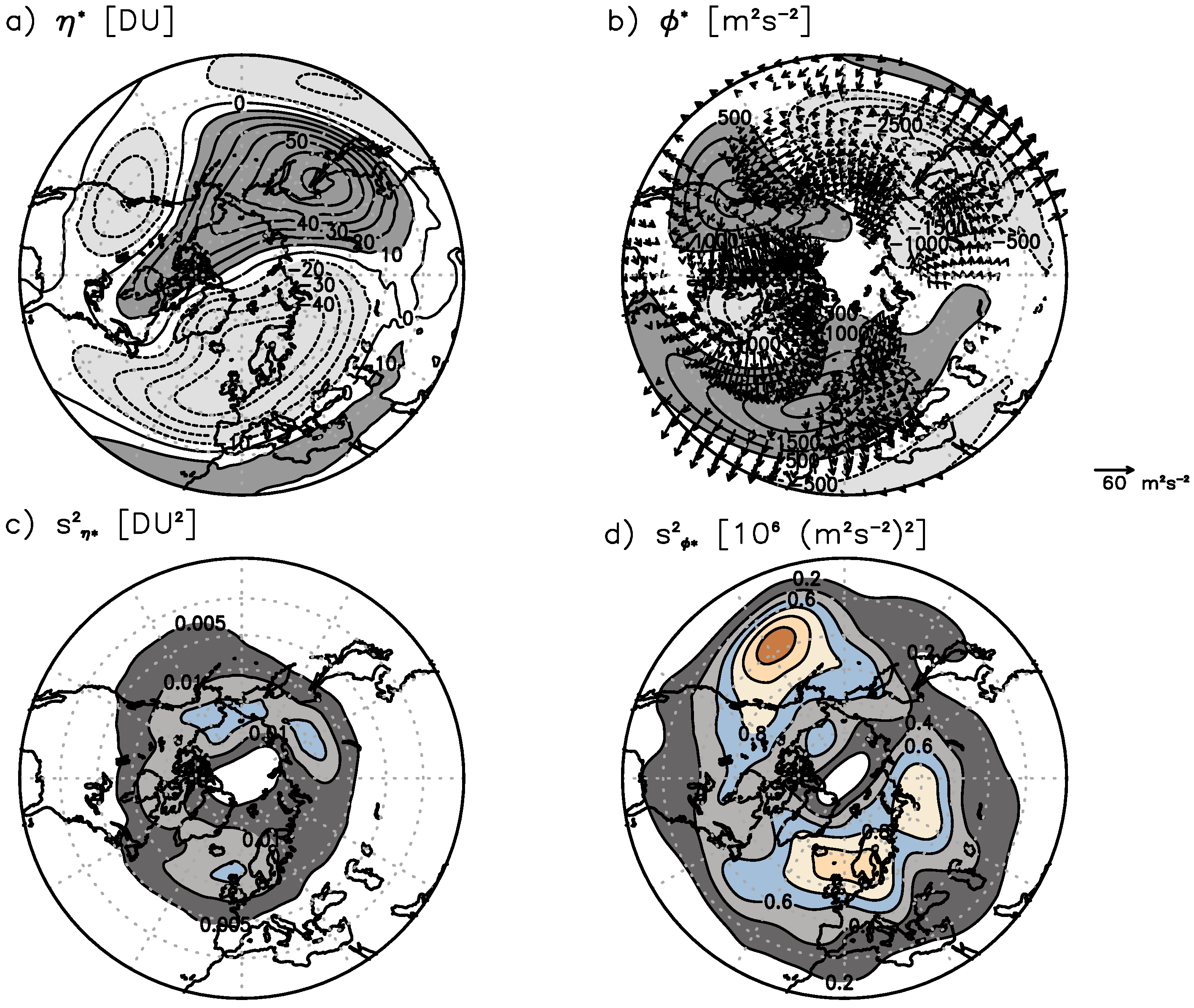
The climatological mean distribution of ZATO for the period 1980–2016 for January (Figure 1a) shows a pronounced wave 1 structure in high latitudes with a minimum over the North Atlantic and a maximum over eastern Siberia, Alaska and Northern Canada. Additionally, a wave 2 structure in ZATO occurs in mid-latitudes with a secondary minimum over the west coast of North America, a secondary maximum over Northeastern Canada, a dominant minimum over North Atlantic/European region and a pronounced maximum over the East Asia/western North Pacific region. The mean distributions for December, February, and the whole winter season (December–January–February, DJF) are close to the January distribution with lower amplitudes (not shown) in agreement with the mean structure identified for the TOMS period [25]. The January variance of ZATO (Figure 1c) increases north of 60° N, with three centers of activity: Over Bering Street, East Siberia and Northeast Atlantic.

ZATO and the geopotential disturbance at 300 hPa (Figure 1b) are well anti-correlated with −0.73 for the Northern Hemisphere. This anti-correlation is manifested in the anti-correlated structure with a dominant anticyclonic disturbance over the North Atlantic/European region and over the west coast of North America. The dominant cyclonic disturbance occurs over the East Asia/North Pacific region and the weaker one occurs over Northeast Canada. The mean geopotential structure agrees well with the quasi-stationary wave structure shown by Plumb [33] for a decadal mean (1965–1975). The geopotential variance is strongest in the midlatitudes of the North Pacific Ocean. The center of variability over the eastern North Atlantic is in coherence with the secondary variance maximum of ZATO. In order to show the climatological planetary wave trains, the wave activity flux is determined according to Plumb [33]. The stationary waves of the climatological January (1980–2016) agrees well with the findings of Plumb [33] showing two major wave trains mainly eastward and predominantly equatorward: One starting from Asia across the North Pacific, and the other starting North America across the North Atlantic.

In summary, this shows that the climatological mean ZATO distribution is mainly determined by the climatological mean ultra-long planetary wave structure due to ozone transport of quasi-stationary ultra-long waves [25].

3.1. Observed Trend of the Zonally Asymmetric Ozone during the Three Stages

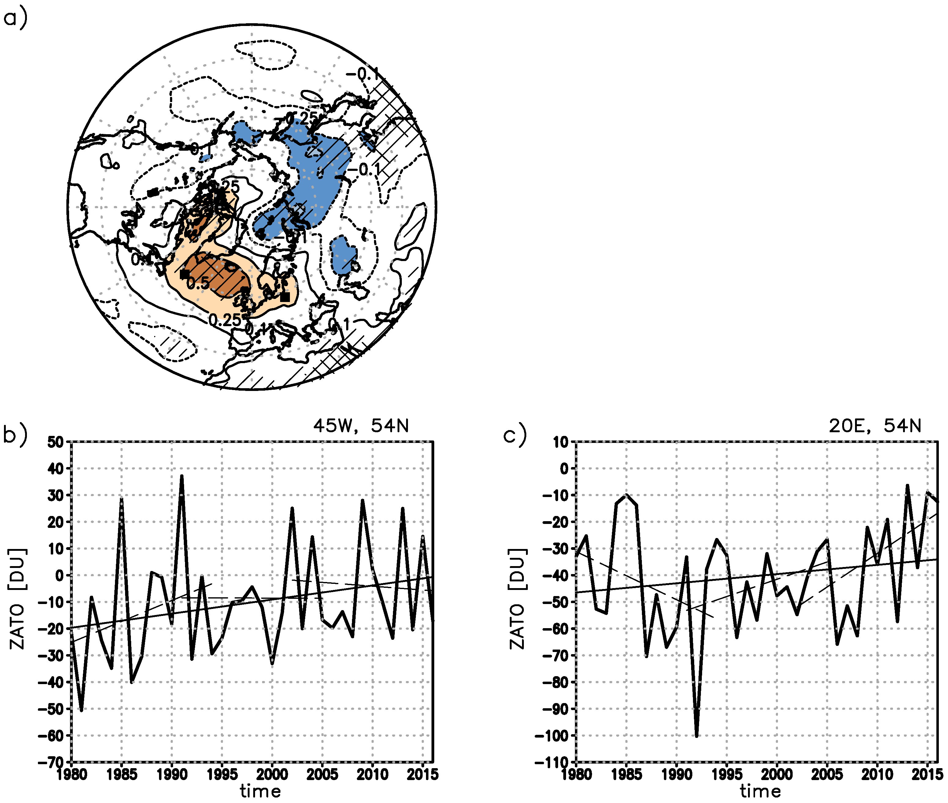
The climatological trend of ZATO for January (1980–2016) is almost small with the greatest changes of 5 DU per decade over the North Atlantic resulting in an increase of roughly 19 DU over the whole period (Figure 2a). However, over Siberia the ZATO decreases by about 9 DU over the whole period. In order to illustrate the different behavior over the North Atlantic/European region during the three stages two significant points with the same latitude of 54° N are selected: One close to the central North Atlantic and the other over Central Europe. Both are located inside the positive ZATO trend pattern (Figure 2a). The ZATO trend over the central North Atlantic (about 5 DU/decade) is a factor of 1.4 stronger than the one over Central Europe (about 3.5 DU/decade) which are shown in Figure 2b,c, respectively.

The secular trends (shown in Figure 2b,c) reveal a strong variability in agreement with Figure 1c and differentiate in each stage. During the healing (decline) stage the trend is positive (negative) over Central Europe and negative (positive) over central North Atlantic (Figure 2c,b). For the leveling stage, the secular trend is weak over the central North Atlantic and positive over Central Europe.

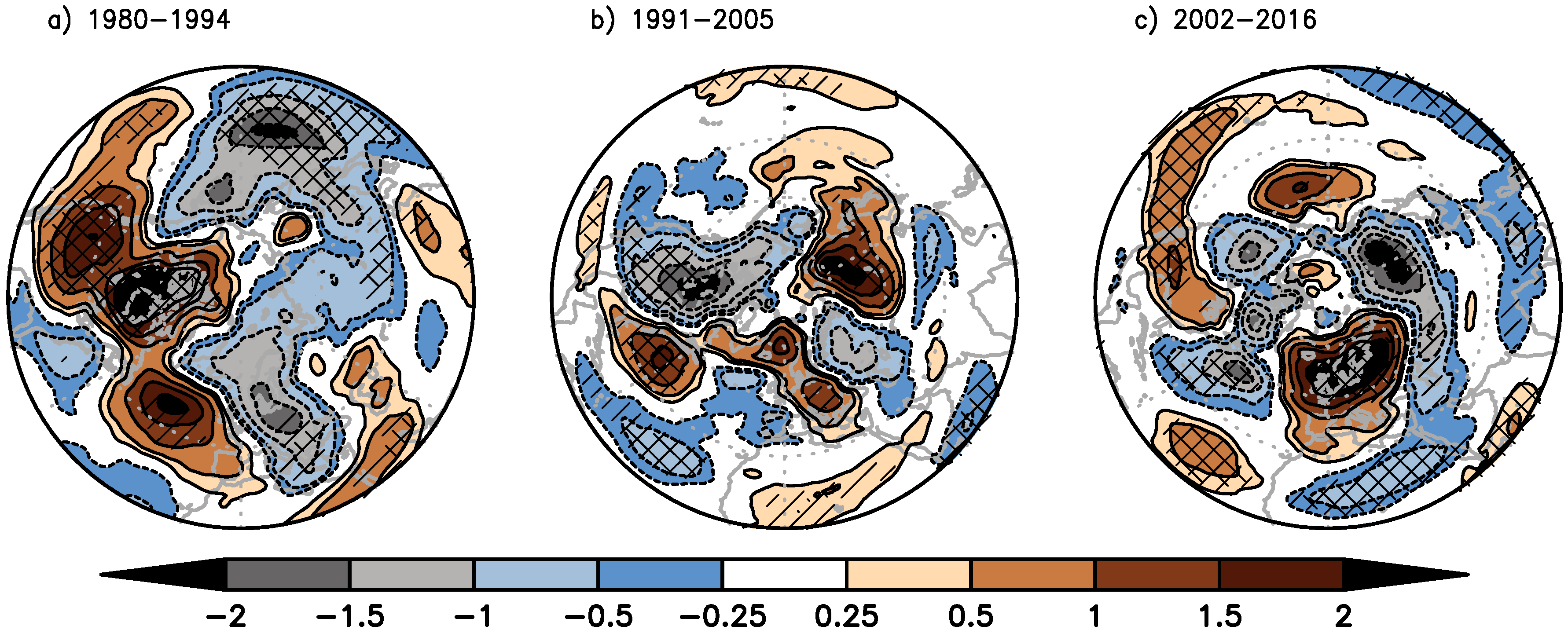
The geographical distribution of the secular trends of ZATO is shown in Figure 3. A simple t-test is applied in order to indicate significant trends. Furthermore, the focus lies on the North Atlantic/European region. The dominant secular trend change of ZATO is located over the North Atlantic/European region as already indicated in Figure 2b,c.

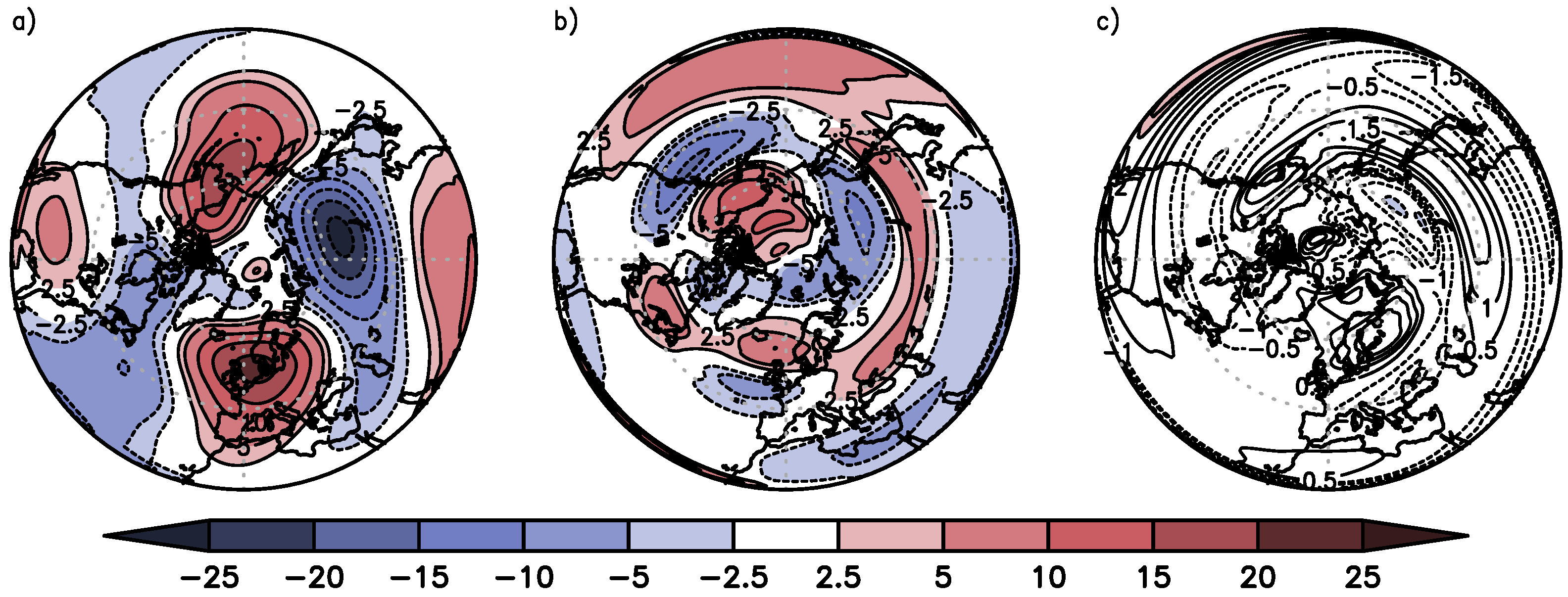
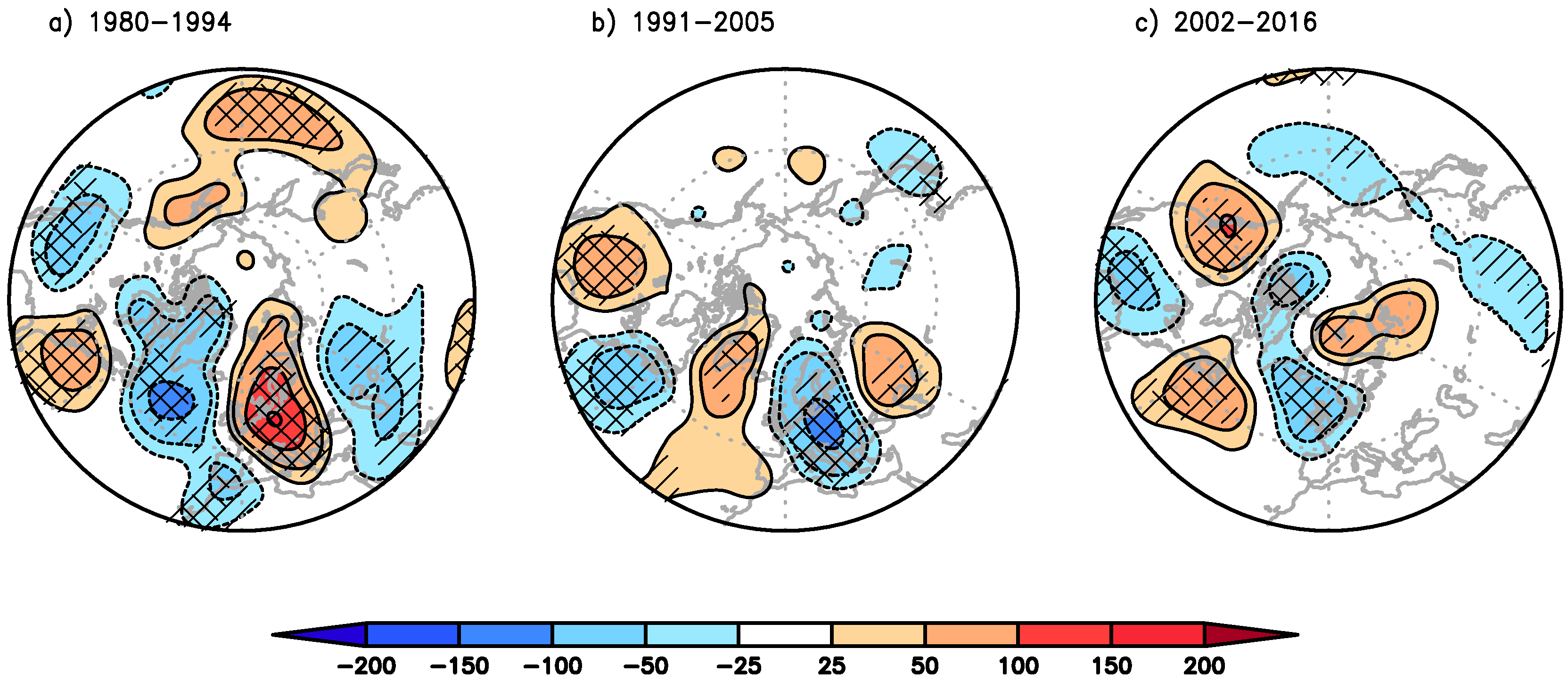
The decline stage for January is characterized by the known wave-like pattern over the North Atlantic/European region (Figure 3a) with a negative trend pattern over eastern North America, a significant positive trend over the North Atlantic, and a significant negative trend over Central Europe. This result is in agreement with previous studies (Hood and Zaff [22] and Peters and Entzian [24,25]). Note that the TOMS period is captured by the decline stage. In addition, significant negative trends of ZATO (about 20 DU/decade) occur over the East Asia/North Pacific region and pronounced positive trends of comparable magnitude over North America and Arctic Canada. The secular trend patterns of ZATO agree well with the regression coefficient of the geopotential disturbances at 300 hPa (Figure 4a) showing an anti-correlated wave pattern over the North Atlantic/European region as expected from former studies [22,24,25]. During December the trend pattern is characterized by a dominant dipole structure with a significant negative trend pattern over the North Atlantic and great parts of Europe and with a positive trend pattern over North America and the Bering Sea (Figures S2a, S6a and S8a; Supplemental Material). During February positive ZATO changes occur over the North Atlantic/European region and negative changes over Eastern Asia and the eastern North Pacific (Figures S3a, S7a and S9a; Supplemental Material). Note that during the decline stage most of the significant changes occur over midlatitudes during DJF. The corresponding secular trends of the geopotential disturbances at 300 hPa shows the establishment of the wave train-like changes, mentioned for January (Figure 4), in December (Figure S4a; Supplemental Material) and the disappearance in February (Figure S5a; Supplemental Material).

During the healing stage, the ZATO trend over western North Atlantic becomes significantly negative and significantly positive over Europe with 20 DU per decade (Figure 3c) in comparison to the decline stage (Figure 3a). Analog changes are observed for the geopotential disturbances (Figure 4) for January.

The wave train over the North Atlantic/European region is curved to the south showing a significantly cyclonic disturbance over the Caspian Sea (Figure 4a) for the decline stage. This wave train weakens and changes its sign during the leveling stage. However, during the healing stage the wave train shifts westward and curves northwards inducing enhanced ageostrophic winds over Europe which implies a strong vertical wind component.

During December (Figures S2c, S6c and S8c; Supplemental Material) the ZATO trend pattern is dominated by a dipole structure over the Arctic with significant positive secular trends over Europe and the Eastern Arctic and significant negative trends over the western Artic and the Bering Sea, which agrees well with the trend pattern of the geopotential disturbances (Figure S4c; Supplemental Material). During February the overall picture is more complex and dominated by small-scale features (Figures S3c, S7c and S9c; Supplemental Material). The trend patterns of the geopotential disturbance for February (Figure S5c; Supplemental Material) show the wave train-like pattern similar to the January distribution of the decline stage (Figure 4a).

During the leveling stage, the secular trends of ZATO (Figure 3b, and Figures S2b and S3b; Supplemental Material) appear more complex, as expected. The geopotential disturbance reveals a significant inverse pattern over the North Atlantic/European region in comparison to the decline stage (Figure 4a,b) for January.

In summary, a huge change of the patterns occurs over the North Atlantic/European region if the evolution over the last 4 decades is taken into account. Often secular patterns show a wave train structure over the North Atlantic/European region in January and dipole structures elsewhere. For December and January the secular trends show a concentration towards the Arctic in the ZATO changes, while for February the secular trends ZATO remain with the focus on midlatitudes.

3.2. Modelled Secular Trends Using the Linearized Transport Equation

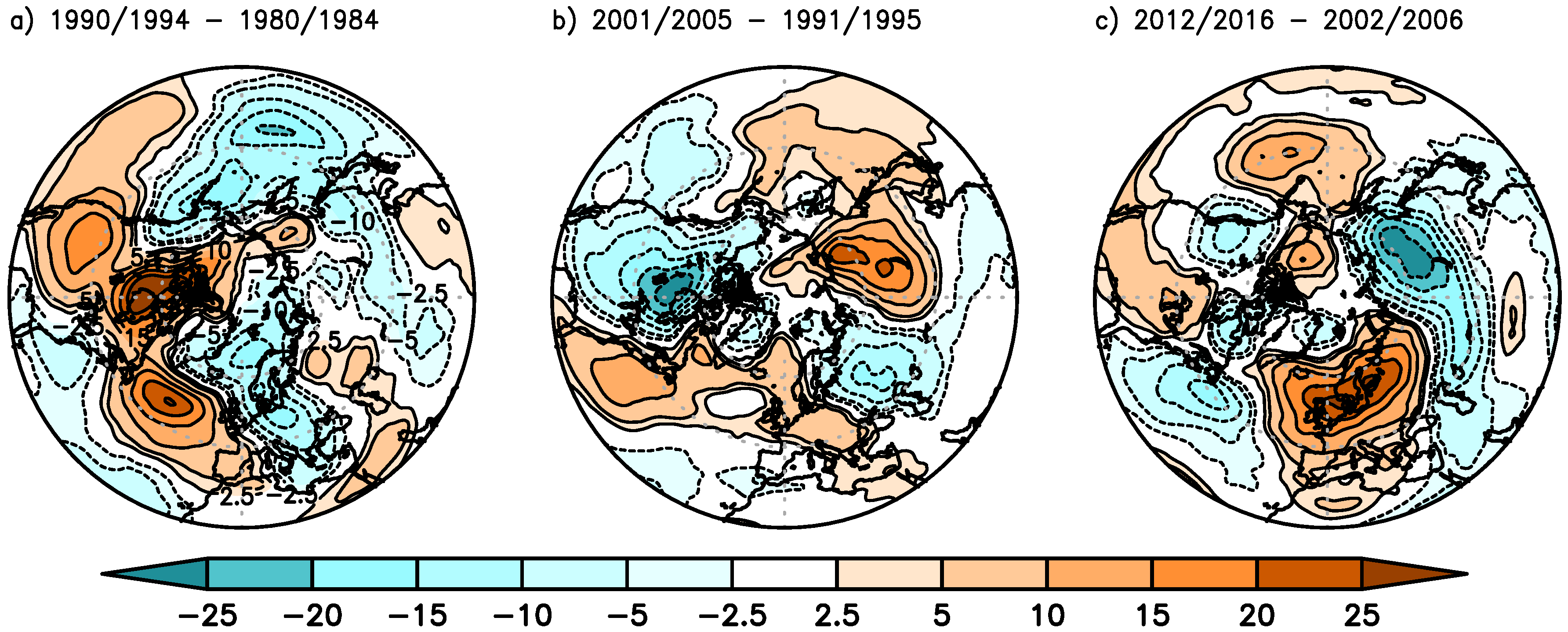
Following [25], the difference between 5-year means of ZATO are used as a proxy for the secular trends of the three stages. These differences are shown in Figure 5. In general, the secular trend patterns (Figure 3) agree very well with the difference pattern (cf. Figure 5; of about 90% coherence with a variability of 4 % between stages). This is in good agreement with [25] for the TOMS period. This statement also holds qualitatively for December and February (Figure S6 for December and Figure S7 for February).

The dominant secular trend patterns of ZATO as well as the wave train structure are very well captured for the North Atlantic/European region in all three stages.

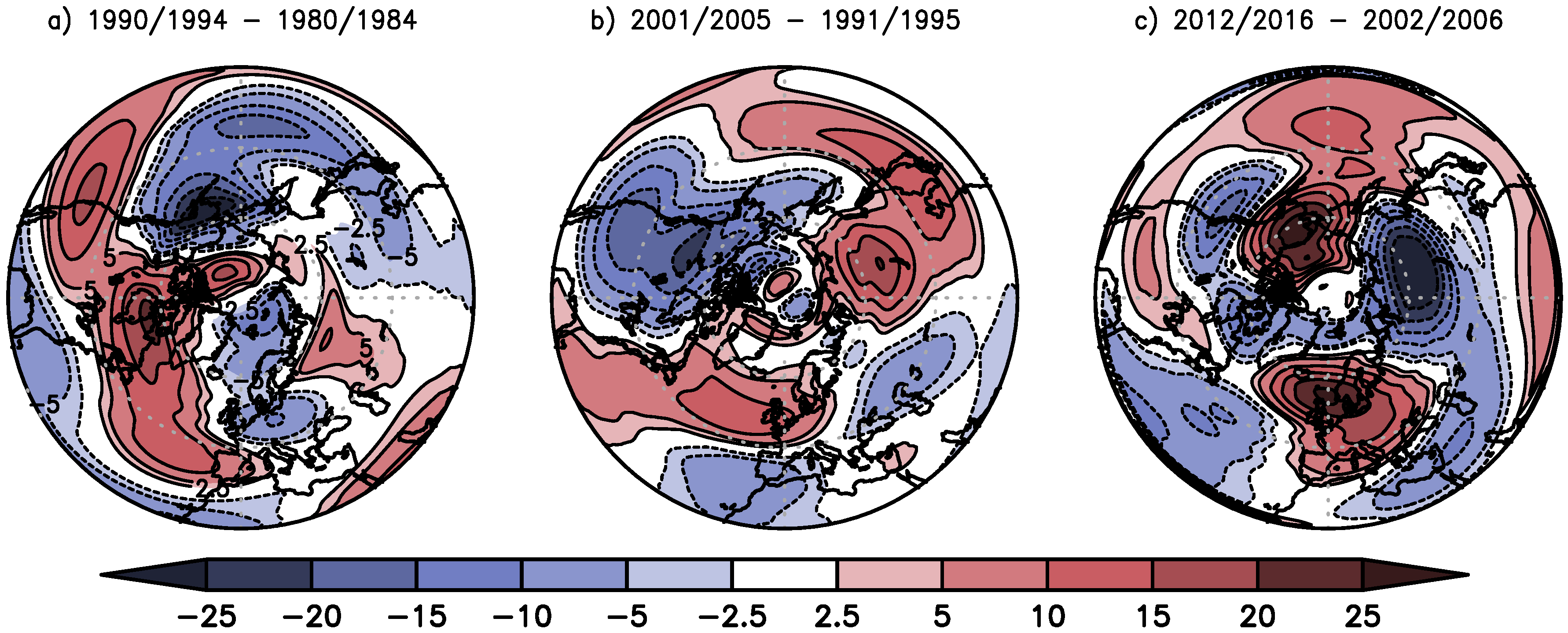
In the next step, the stationary transport Equation (3) is solved by using given harmonic components of geopotential disturbances and temperature; and zonal mean winds and zonal mean ozone from ERA-Interim for each 5-year mean of periods. Only ultra-long waves with zonal wave numbers 1 to 4 are considered and finally superposed. The differences of ZAO for each stage are calculated together with the boreal distribution of ZATO (shown in Figure 6).

The comparison between transport model results (Figure 6) and observation of trend-like behavior (Figure 5) reveals a good pattern coherence. For the whole Northern Hemisphere between 50% to 60% can be explained with the transport by ultra-long waves as shown in

Table 1. Pattern correlation of the trend-like pattern of ZATO for 25° N–90° N for observations using ERA-Interim source data (obs) and the linear model results using Equation (3) (mod).

Pattern Correlation	Decline	Leveling Off	Healing
	(1990/1994–1980/1984)	(2001/2005–1991/1995)	(2012/2016–2002/2006)
obs & mod	0.78	0.73	0.71
obs & ClimEta	0.88	0.79	0.77
obs & ClimWav	0.02	−0.03	0.23
obs & ANO	−0.21	0.26	0.35
obs & ClimEta + ClimWave	0.78	0.73	0.72
obs & ClimEta + ANO	0.86	0.78	0.78

(first row). The pattern changes of ZATO over the North Atlantic/European region are well captured not only during the healing stage. The greatest differences occur close to the Arctic and Eastern Europe. The calculated trend (Figure 6) shows stronger positive trends over Alaska and stronger negative trends over Siberia indicating an overestimation during the healing stage.

The secular trends calculated with the transport model for December and February are shown in Figures S8 and S9 (supplemental material), respectively.

In summary, for North Atlantic/European region the calculated secular trends for the healing stages are very similar for December and January, with higher absolute values in January but weaker for February.

In the next subsections, the linear transport model is used to quantify the contributions of the horizontal and vertical wave transport of ozone following [25]. Then, the importance of climatological and anomaly transport is examined following Equations (4)–(6).

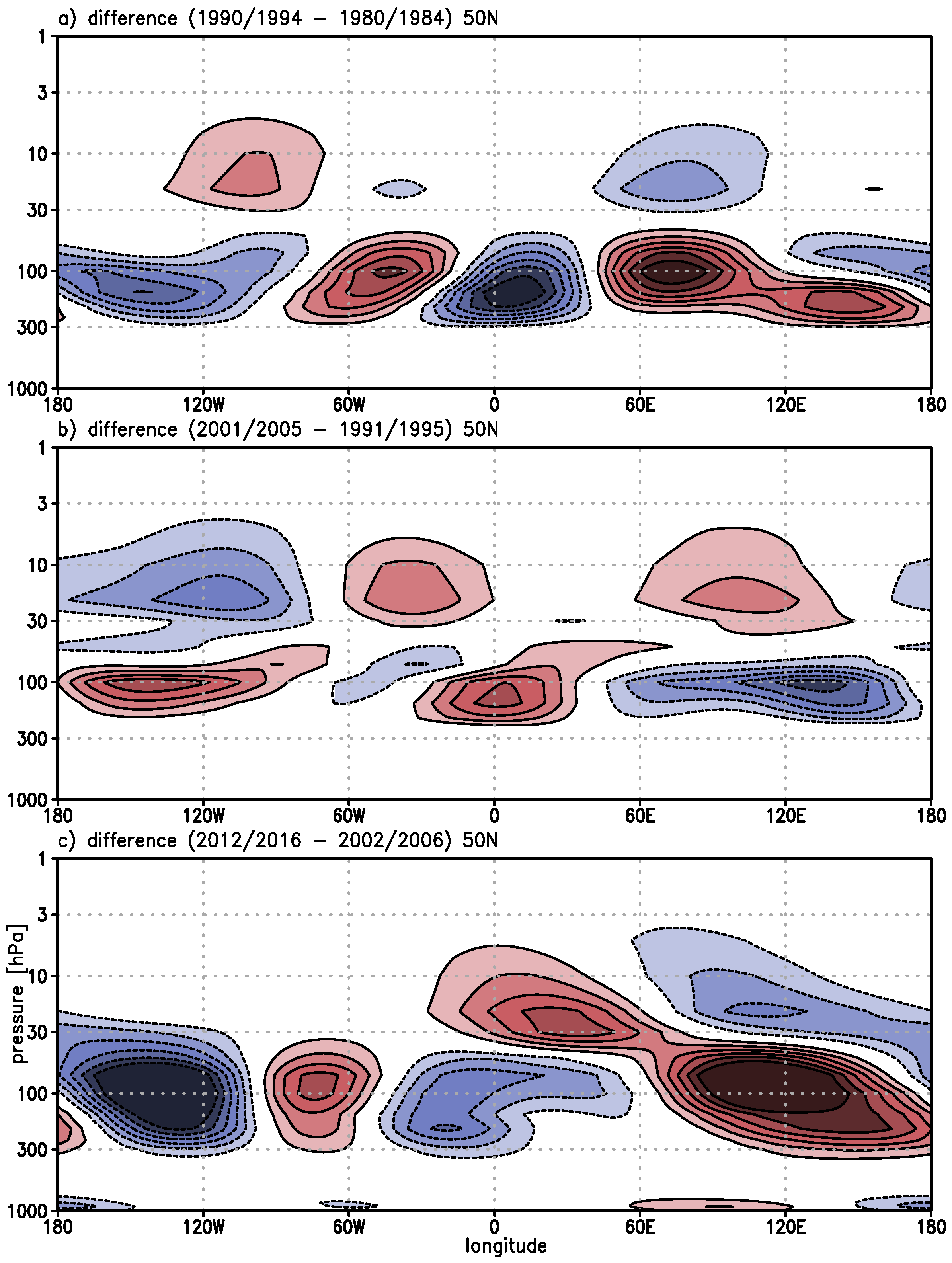
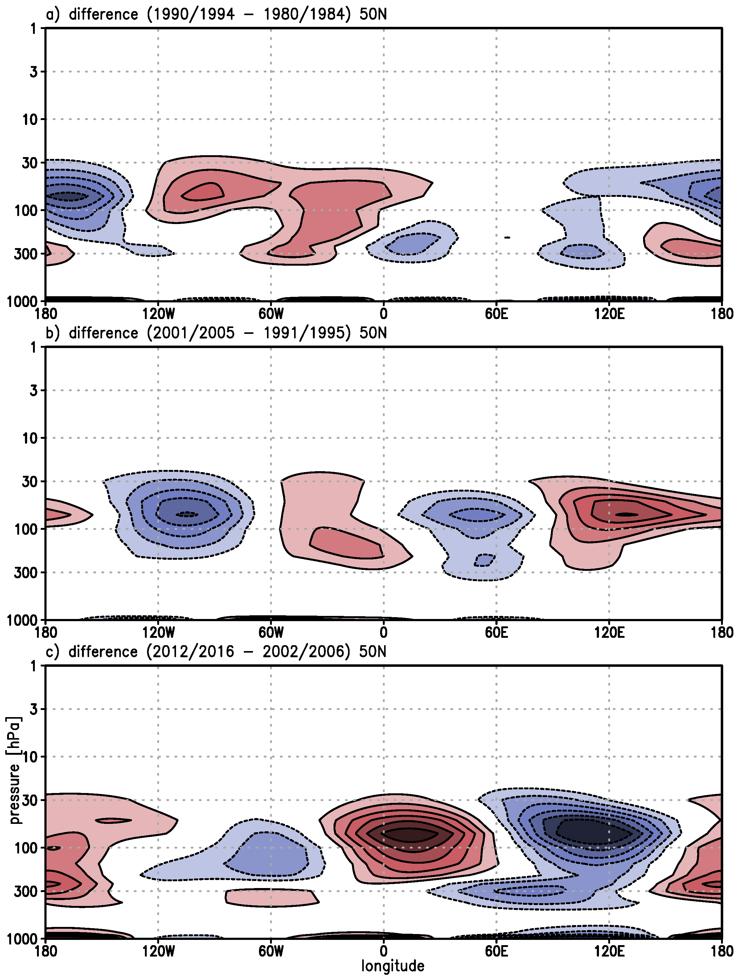
3.2.1. Contributions of the Horizontal and Vertical Advection

Following [25] the secular trend-like contribution of the horizontal and vertical advection of ozone to ZAO distribution are examined with the help of Equation (3) for all three stages. Cross-sections for a typical midlatitude (50° N, Figure 7 and Figure 8) show a wave-like structure as expected in the whole stratosphere.

During the decline stage, the horizontal advection of ozone dominates in the lower stratosphere over the North Atlantic/European region (Figure 7a). For the leveling stage, the distribution shows a decrease in the lower stratosphere and an increase in the middle stratosphere over the same region. During the healing stage, the horizontal advection of ozone is reduced in the lower stratosphere of the North Atlantic/European region. The centers are shifted westward by about 30 degrees. Over Europe, the horizontal transport increases in the middle stratosphere. The horizontal advection of ozone dominates over eastern Siberia and eastern North Pacific in the lower stratosphere. The vertical transport of ozone (second term of Equation (3), Figure 8) shows weaker values (roughly 50%) in comparison to the horizontal advection of ozone (Figure 7). The upward advection of ozone dominates in the lower stratosphere over the North Atlantic during the decline stage, also found by Peters and Entzian [25] for the TOMS period. However, during the healing stage, this pattern is shifted eastwards to Europe and shows an increase by a factor of about 3 in its center placed in the lower stratosphere.

During the healing stage, the dominant ZATO trend is positive over Europe (Figure 6c) which is mainly caused by the increase of vertical advection of ozone in the lower stratosphere (Figure 8c) in comparison to the horizontal advection of ozone which is weak in the vertical integral (Figure 7c). This increase of the vertical ozone transport over Europe indicates an increase of the ageostrophic advection of ozone, which is discussed in more detail in Section 4.

3.2.2. Contributions Due to Climate and Anomalies

The separation of geopotential, temperature, and zonal mean ozone into its climatological and anomaly part (Equations (4)–(6), Section 2.2) gives a more detailed physical inside as discussed by [34].

The different contributions derived in Equations (4)–(6) are shown in Figure 9 for the healing stage, only. The secular positive ozone trend over Europe (ClimEta, Equation (4), Figure 9a) is mainly determined by the anomalous quasi-stationary wave transport of ultra-long waves in the frame of the climatological mean ozone in comparison with the other terms (Figure 9b,c). Note the climatological mean ozone field is plotted in Figure S1 of Supplemental Material. During the course of the three stages, this contribution decreases slightly but remains the most important contribution (not shown). The secular trend contribution of the climatological quasi-stationary wave transport in the frame of zonal mean ozone anomalies (ClimWav, Equation (5)) shows a dipole structure over the eastern North Atlantic/European region, which additionally increases the positive ozone trend over the Norwegian Sea (Figure 9b). The eastward extension of the positive ozone trend over Eastern Europe is supported by the correlation between both, wave and ozone anomaly (ANO, Equation (6)), but it is weaker (Figure 9c).

The results of a pattern correlation between the calculated physical contributions (Figure 9) and the calculated secular trend (Figure 6) are given in Table 1.

In general, for all three stages the main contribution comes from the anomalous quasi-stationary wave transport of climatological mean ozone (ClimEta, cf. Table 1). However, during the course of the three stages this contribution decreases slightly but remains the most important contribution. The highest pattern correlation is given if the contribution of the interaction between anomalous quasi-stationary waves and the anomalous zonal mean ozone (ANO term) is added (last row in Table 1) explaining about 60% of the trend pattern (Figure 6).

4. Discussion

This investigation shows that the boreal climatological mean ZATO distribution for the period (1980–2016) is strongly anti-correlated to the climatological mean ultra-long wave structure at 300 hPa with a high variability of both over the North Atlantic/European region (Figure 1). Transport of ozone by quasi-stationary ultra-long waves without the consideration of chemistry almost explains the structure of climatological ZATO (not shown) in agreement with former studies [23].

The climatological trend of ZATO for January (1980–2016) is relatively small with the greatest changes of 5 DU per decade over the North Atlantic resulting in an increase of roughly 19 DU over the whole period of about 4 decades (Figure 2a). The secular trends (Figure 2b,c) reveal a strong variability in that region as also shown in Figure 1c. During the decline stage, the ZATO trend is significantly negative over Central Europe and significantly positive over the central North Atlantic (Figure 1b) for January. This finding confirms the results of Hood and Zaff [22] and Peters et al. [23] for January of the TOMS period.

One main finding of the study is that during the healing stage in January, the ZATO trend turns around, that means a significantly positive trend over Central Europe and significantly negative trend over the central North Atlantic (Figure 2b,c and Figure 3) occur.

The December evolution of ZATO trend also turns around over Northern Europe during the healing stage, but stays with negative trend over South Europe. For February, the ZATO trends are weaker and a very complex trend structure occurs (Figures S2c and S3c; Supplemental Material).

During the healing stage, a superposition of these secular trends for mean winter months is dominated by the January-trend pattern with a poleward shift due to the December-trend pattern over the North Atlantic/European region. This pattern is in agreement with the results of Zhang et al. ([27], their Figure 3c,d) also showing a change from a negative to a positive trend pattern over northern Europe from the period (1979–1997) to (1997–2015) for winter mean.

The used stationary linear transport model of ozone is applicable for the three stages. This implies the assumption that photochemistry can be neglected during the winter for the lower stratosphere, which results from the much slower time scale of chemistry in comparison with the time scale of the advective processes by the large-scale waves. During the healing stage, the calculated dominant ZATO trend is positive over Europe (Figure 6c) which is mainly caused by the increase of the vertical advection of ozone in the lower stratosphere (Figure 8c) in comparison to the horizontal advection of ozone which is weak after vertical integration (Figure 7c). This increase of the vertical ozone transport over Europe indicates an increase of the ageostrophic advection of ozone. In the quasi-geostrophic theory [30], which holds for ultra-long waves, it can be shown that the vertical advection is equivalent to the ageostrophic horizontal wind advection.

During the healing stage (2002–2016), the increase of vertical transport of ozone by ultra-long waves determines the secular trend pattern over the North Atlantic/European region, which demonstrates the growing importance of ageostrophic ozone transport. However, the wave train shifts westward and curves northwards inducing these enhanced ageostrophic winds over Europe. The question is where do they come from? It is known, that the Artic indicates a strong warming during the healing stage, which is mainly caused by atmospheric heat transport in winter [35]. Interdecadal changes of the Madden-Julian Oscillation (MJO), the most prominent mode of intraseasonal variability in the tropics, could also contribute to the Arctic warming. [36] show that interdecadal changes of the MJO towards a higher frequency of phases 4–6 contribute to the Arctic amplification with 10–20%. This teleconnection can be explained by Rossby wave dynamics excited due to enhanced tropical convection [36,37,38]. Furthermore it is known that Ural blocking has strongly been increased over last decades [39,40]. Both facts are in agreement with our findings of a westward wave train shift and northward curvature during the healing stage.

Furthermore, the separation of different physical contributions of ozone transport (climate and anomaly) reveals that the climatological zonal mean ozone transport by anomalous planetary waves dominates. This implies that changes of the ultra-long wave structure are mainly responsible for the changes of secular trend during all stages.

The contributions of the correlation-anomaly term (ANO) should be included because it improves the pattern correlation up to 60% (Table 1 last row).

5. Conclusions

Strong ZATO changes are observed in the boreal extratropics for winter month January. Recent studies demonstrate that the mean ozone evolution reveals three different quasi-bidecadal (or secular) trend stages: (i) Decline, (ii) leveling, and (iii) healing. Here, the focus lies on the investigation of the ZAO structure in boreal extratropics and on the ozone transport changes by ultra-long waves during the winter months of the last four decades. ERA-Interim data together with a linearized transport model are used. We found that significant ZATO increases over the North Atlantic/European region during the healing stage in comparison to a strong decrease of ZATO during the decline stage for January. The ZATO increase (healing stage) and ZATO decrease (decline stage) are caused by different monthly mean transport characteristics of ultra-long planetary waves over the North Atlantic/European region. Furthermore, the vertical advection (ageostrophic transport) of ozone versus horizontal (geostrophic) dominates in the lower and upper stratosphere during the healing stage. The separation of different physical contributions of ozone transport (climate and anomaly) reveals that the climatological zonal mean ozone transport by anomalous planetary waves dominates.

In general, the changes of the ultra-long wave structure are mainly responsible for the changes of secular trends during all stages. It is hypothesized that ZATO increase over Europe is linked to the Arctic warming by enhancing ageostrophic ozone transport. Additional sensitivity runs for each stage and month with a AGCM (Atmosphere Genereal Circulation Model) are suggested in order to examine the role of the circulation changes in more details during the three stages.

References

1. WMO (World Meteorological Organization). Scientific Assessment of Ozone Depletion. In World Meteorological Organization, Global Ozone Research and Monitoring Project Report; No. 55; WMO: Geneva, Switzerland, 2014; p. 416. [Google Scholar]
2. Stocker, T.F.; Qin, D.; Plattner, G.-K.; Tignor, M.; Allen, S.K.; Boschung, J.; Nauels, A.; Xia, Y.; Bex, V.; Midgley, P.M. (Eds.) IPCC 2013: Climate Change 2013: The Physical Science Basis. Contribution of Working Group I to the Fifth Assessment Report of the Intergovernmental Panel on Climate Change; Cambridge University Press: Cambridge, UK; New York, NY, USA, 2013; p. 1535. [Google Scholar]
3. Ball, W.T.; Alsing, J.; Mortlock, D.J.; Staehelin, J.; Haigh, J.D.; Peter, T.; Tummon, F.; Stübi, R.; Stenke, A.; Anderson, J.; et al. Evidence for a continuous decline in lower stratospheric ozone offsetting ozone layer recovery. Atmos. Chem. Phys. 2018, 18, 1379–1394. [Google Scholar] [CrossRef] [Green Version]
4. Chipperfield, M.P.; Dhomse, S.; Hossaini, R.; Feng, W.; Santee, M.L.; Weber, M.; Burrows, J.P.; Wild, J.D.; Loyola, D.; Coldewey-Egbers, M. On the Cause of Recent Variations in Lower Stratospheric Ozone. Geophys. Res. Lett. 2018, 45, 5718–5726. [Google Scholar] [CrossRef]
5. WMO (World Meteorological Organization). Scientific Assessment of Ozone Depletion. In Global Ozone Research and Monitoring Project-Report; No. 50; WMO: Geneva, Switzerland, 2006; p. 572. [Google Scholar]
6. Solomon, S.; Ivy, D.J.; Kinnison, D.; Mills, M.J.; Neely, R.R.; Schmidt, A. Emergence of healing in the Antarctic ozone layer. Science 2016, 353, 269–274. [Google Scholar] [CrossRef] [PubMed] [Green Version]
7. Chipperfield, M.P.; Bekki, S.; Dhomse, S.; Harris, N.R.P.; Hassler, B.; Hossaini, R.; Steinbrecht, W.; Thiéblemont, R.; Weber, M. Detecting recovery of the stratospheric ozone layer. Nature 2017, 549, 211–218. [Google Scholar] [CrossRef] [PubMed] [Green Version]
8. Andrews, D.G.; Holton, J.R.; Leovy, C.B. Middle Atmosphere Dynamics; Academic Press: New York, NY, USA, 1987; p. 489. [Google Scholar]
9. Albers, J.R.; Nathan, T.R. Pathways for communicating the effects of stratospheric ozone to the polar vortex: Role of zonally asymmetric ozone. J. Atmos. Sci. 2012, 69, 785–801. [Google Scholar] [CrossRef]
10. Sassi, F.; Boville, B.A.; Kinnison, D.; Garcia, R.R. The effects of interactive ozone chemistry on simulations of the middle atmosphere. Geophys. Res. Lett. 2005, 32, L07811. [Google Scholar] [CrossRef]
11. Kirchner, I.; Peters, D. Modelling the wintertime response to upper tropospheric and lower stratospheric ozone anomalies over the North Atlantic and Europe. Ann. Geophys. 2003, 21, 2107–2118. [Google Scholar] [CrossRef] [Green Version]
12. Gabriel, A.; Peters, D.; Kirchner, I.; Graf, H.-F. Effect of zonally asymmetric ozone on stratospheric temperature and planetary wave propagation. Geophys. Res. Lett. 2007, 34, L06807. [Google Scholar] [CrossRef]
13. Crook, J.A.; Gillett, N.P.; Keeley, S.P.E. Sensitivity of Southern Hemisphere climate to zonal asymmetry in ozone. Geophys. Res. Lett. 2008, 35, L07806. [Google Scholar] [CrossRef]
14. Gillett, N.P.; Scinocca, J.F.; Plummer, D.A.; Reader, M.C. Sensitivity of climate to dynamically-consistent zonal asymmetries in ozone. Geophys. Res. Lett. 2009, 36, L10809. [Google Scholar] [CrossRef]
15. Waugh, D.W.; Oman, L.; Newman, P.A.; Stolarski, R.S.; Pawson, S.; Nielsen, J.E.; Perlwitz, J. Effect of zonal asymmetries in stratospheric ozone on simulated Southern Hemisphere climate trends. Geophys. Res. Lett. 2009, 36, L18701. [Google Scholar] [CrossRef]
16. Waugh, D.W.; Garfinkel, C.I.; Polvani, L.M. Drivers of the recent tropical expansion in the Southern Hemisphere: Changing SSTs or ozone depletion? J. Clim. 2015, 28, 6581–6586. [Google Scholar] [CrossRef]
17. Dennison, F.; McDonald, A.; Morgenstern, O. The evolution of zonally asymmetric austral ozone in a chemistry-climate model. Atmos. Chem. Phys. 2017, 17, 14075–14084. [Google Scholar] [CrossRef]
18. Garcia, R.R.; Hartmann, D.L. The role of planetary waves in the maintenance of zonally averaged ozone distrubution of the upper stratosphere. J. Atmos. Sci. 1980, 37, 2248–2264. [Google Scholar] [CrossRef]
19. Nathan, T.R. On the role of ozone in the stability of Rossby normal modes. J. Atmos. Sci. 1989, 46, 2094–2100. [Google Scholar] [CrossRef]
20. Nathan, T.R.; Cordero, E.C. An ozone-modified refractive index for vertically propagating planetary waves. J. Geophys. Res. 2007, 112, D02105. [Google Scholar] [CrossRef]
21. Peters, D.H.W.; Schneidereit, A.; Bügelmayer, M.; Zülicke, C.; Kirchner, I. Atmospheric circulation changes in response to observe stratospheric zonal ozone anomaly. Atmos.-Ocean 2015, 53, 74–88. [Google Scholar] [CrossRef]
22. Hood, L.L.; Zaff, D.A. Lower stratospheric stationary waves and the longitude dependence of ozone trends in winter. J. Geophys. Res. 1995, 100, 25791–25800. [Google Scholar] [CrossRef]
23. Peters, D.; Entzian, G.; Schmitz, G. Ozone anomalies over the North Atlantic-European region during January 1979–1992—Linear modelling of horizontal and vertical ozone transport by ultra-long waves. Beitr. Phys. Atmos. 1996, 69, 477–489. [Google Scholar]
24. Peters, D.; Entzian, G. January ozone anomaly over the North Atlantic-European region: Longitude-dependent decadal change in the total ozone during 1979–1992. Meteorol. Z. 1996, 5, 41–44. [Google Scholar] [CrossRef]
25. Peters, D.; Entzian, G. Longitude-Dependent Decadal Changes of Total Ozone in Boreal Winter Months during 1979–1992. J. Clim. 1999, 12, 1038–1048. [Google Scholar] [CrossRef]
26. Peters, D.H.W.; Gabriel, A.; Entzian, G. Longitude-dependent decadal ozone changes and ozone trends in boreal winter months during 1960–2000. Ann. Geophys. 2008, 26, 1275–1286. [Google Scholar] [CrossRef]
27. Zhang, J.; Tian, W.; Xie, F.; Sang, W.; Guo, D.; Chipperfield, M.; Feng, W.; Hu, D. Zonally asymmetric trends of winter total column ozone in the northern middle latitudes. Clim. Dyn. 2018, 1–8. [Google Scholar] [CrossRef]
28. Dee, D.P.; Uppala, S.M.; Simmons, A.J.; Berrisford, P.; Poli, P.; Kobayashi, S.; Andrae, U.; Balmaseda, M.A.; Balsamo, G.; Bauer, P.; et al. The ERA-Interim reanalysis: Configuration and performance of the data assimilation system. Q. J. R. Meteorol. Soc. 2011, 137, 553–597. [Google Scholar] [CrossRef]
29. Rienecker, M.M.; Suarez, M.J.; Gelaro, R.; Todling, R.; Bacmeister, J.; Liu, E.; Bosilovich, M.G.; Schubert, S.D.; Takacs, L.; Kim, G.-K.; et al. MERRA: NASA’s Modern-Era Retrospective Analysis for Research and Applications. J. Clim. 2011, 24, 3624–3648. [Google Scholar] [CrossRef]
30. Holton, J.R. Equatorial Wave-Mean Flow Interaction: A Numerical Study of the Role of Latitudinal Shear. J. Atmos. Sci. 1979, 36, 1030–1040. [Google Scholar] [CrossRef] [Green Version]
31. Taubenheim, J. Statistische Auswertung Geophysikalischer und Meteorologischer Daten; Akademische Verlagsgesellschaft Geest: Portig, Leipzig, Germany, 1969; p. 380. [Google Scholar]
32. Kurzeja, R.J. Spatial variability of total ozone at high latitudes in winter. J. Atmos. Sci. 1984, 41, 695–697. [Google Scholar] [CrossRef]
33. Plumb, R.A. On the Three-Dimensional Propagation of Stationary Waves. J. Atmos. Sci. 1985, 42, 217–229. [Google Scholar] [CrossRef] [Green Version]
34. Schneidereit, A.; Peters, D.H.W.; Grams, C.M.; Quinting, J.F.; Keller, J.H.; Wolf, G.; Teubler, F.; Riemer, M.; Martius, O. Enhanced Tropospheric Wave Forcing of Two Anticyclones in the Prephase of the January 2009 Major Stratospheric Sudden Warming Event. Mon. Weather Rev. 2017, 145, 1797–1815. [Google Scholar] [CrossRef]
35. Perlwitz, J.; Hoerling, M.; Dole, R. Arctic Tropospheric Warming: Causes and Linkages to Lower Latitudes. J. Clim. 2015, 28, 2154–2167. [Google Scholar] [CrossRef]
36. Yoo, C.; Feldstein, S.; Lee, S. The impact of the Madden-Julian Oscillation trend on the Arctic amplification of surface air temperature during the 1979–2008 boreal winter. Geophys. Res. Lett. 2011, 38, L24804. [Google Scholar] [CrossRef]
37. Yoo, C.; Lee, S.; Feldstein, S.B. Mechanisms of Arctic surface air temperature change in response to the Madden-Julian Oscillation. J. Clim. 2012, 25, 5777–5790. [Google Scholar] [CrossRef]
38. Seo, K.-H.; Lee, H.-J.; Frierson, D.M.W. Unraveling the teleconnection mechanisms that induce wintertime temperature anomalies over the Northern Hemisphere continents in response to the MJO. J. Atmos. Sci. 2016, 73, 3557–3571. [Google Scholar] [CrossRef]
39. Yao, Y.; Luo, D.; Dai, A.; Simmonds, I. Increased Quasi Stationarity and Persistence of Winter Ural Blocking and Eurasian Extreme Cold Events in Response to Arctic Warming. Part I: Insights from Observational Analyses. J. Clim. 2017, 30, 3549–3568. [Google Scholar] [CrossRef]
40. Luo, D.; Yao, Y.; Dai, A.; Simmonds, I.; Zhong, L. Increased Quasi Stationarity and Persistence of Winter Ural Blocking and Eurasian Extreme Cold Events in Response to Arctic Warming. Part II: A Theoretical Explanation. J. Clim. 2017, 30, 3569–3587. [Google Scholar] [CrossRef]
41. Berrisford, P.; Dee, D.P.; Poli, P.; Brugge, R.; Fielding, M.; Fuentes, M.; Kåallberg, P.W.; Kobayashi, S.; Uppala, S.; Simmons, A. The ERA-Interim Archive Version 2.0; ERA Report; Shinfield Park: Reading, UK, 2011. [Google Scholar]
Figure 1. Climatological mean of (a) zonally asymmetric total ozone (ZATO) [DU] and of the (b) geopotential disturbance [m2 s−2] at 300 hPa for January 1980–2016. The variances are shown for (c) ZATO [DU2] and for (d) the geopotential disturbance [m4 s−4]. Additionally, arrows in (b) indicate the wave activity flux vector according to [33] in [m2 s−2].
Atmosphere 09 00468 g001
Figure 2. Linear regression coefficient (trend) for (a) ZATO for January (1980–2016) in [DU/year]. Crossed (single) hatched regions mark statistically significant trends on a 95% (90%) confidence level. Contour interval in (a) is in absolute values 0.1 , 0.25 , 0.5 . Black filled squares in (a) marks two points. The time series of ZATO [DU] are plotted in (b) for 45° W, 54° N, and in (c) for 20° E, 54° N. The solid straight line indicates the linear regression over the whole period (climatological trend). Dashed lines in (b,c) indicate the secular trends for each stage.
Atmosphere 09 00468 g002
Figure 3. Secular trends (linear regression coefficient) of ZATO in [DU/year] for the three stages: (a) 1980–1994, (b) 1991–2005, and (c) 2002–2016 for January. Cross (single) hatched regions mark statistically significant trends on a 95% (90%) confidence level.
Atmosphere 09 00468 g003
Figure 4. Secular trends (linear regression coefficient) of the geopotential disturbance at 300 hPa in [m2 s−2/year] for the three stages: (a) 1980–1994, (b) 1991–2005, and (c) 2002–2016 for January ERA-Interim. Cross (single) hatched regions mark statistically significant trends with a 95% (90%) confidence level.
Atmosphere 09 00468 g004
Figure 5. Trend-like pattern determined by the difference of 5-year means of ZATO for January. The three different stages are described by the following differences (a) 1990/1994–1980/1984, (b) 2001/2005–1991/1995, (c) 2012/2016–2002/2006. Note that the unit of the difference is DU/decade.
Atmosphere 09 00468 g005
Figure 6. Trend-like pattern determined by the difference of 5-year means of ZATO in [DU/decade] for January but using the linear transport model results with contributions of wave 1–4.
Atmosphere 09 00468 g006
Figure 7. Model result: Pressure-longitude cross-section of the horizontal advection (first term of Equation (3), [DU/km]) at 50° N for January based on differences of different periods: (a)1990/1994–1980/1984, (b) 2001/2005–1991/1995, and (c) 2012/2016–2002/2006. Absolte values above 0.2 DU/km are shaded with a contour interval 0.2.
Atmosphere 09 00468 g007
Figure 8. Similar to Figure 7 for the vertical advection (second term of Equation (3)). Absolte values above 0.2 DU/km are shaded with a contour interval 0.2.
Atmosphere 09 00468 g008
Figure 9. Different contributions of the calculated trend-like pattern of the zonally asymmetric total column ozone in [DU/decade] during the healing stage (2012/2016–2002/2006): (a) ClimEta, (b) ClimWav, and (c) ANO. Only contributions of wave 1–4 are considered.
Atmosphere 09 00468 g009