Article

PM2.5 Chemical Compositions and Aerosol Optical Properties in Beijing during the Late Fall

1
Key Laboratory of Reservoir Aquatic Environment of CAS, Chongqing Institute of Green and Intelligent Technology, Chinese Academy of Sciences, Chongqing 400714, China
2
School of Chemistry and Environment, Beihang University, Beijing 100191, China
3
Key Lab of Aerosol Chemistry & Physics, Institute of Earth Environment, Chinese Academy of Sciences, Xi'an 710075, China
4
School of Physics, Peking University, Beijing 100871, China
5
State Environmental Protection Key Laboratory of Sources and Control of Air Pollution Complex, School of Environment, Tsinghua University, Beijing 100084, China
*
Author to whom correspondence should be addressed.
Atmosphere 2015, 6(2), 164-182; https://doi.org/10.3390/atmos6020164
Submission received: 21 November 2014 / Revised: 31 December 2014 / Accepted: 7 January 2015 / Published: 26 January 2015
(This article belongs to the Special Issue Sources, Formation and Impacts of Secondary Aerosol)

Abstract

:
Daily PM2.5 mass concentrations and chemical compositions together with the aerosol optical properties were measured from 8–28 November 2011 in Beijing. PM2.5 mass concentration varied from 15.6–237.5 μg∙m−3 and showed a mean value of 111.2 ± 73.4 μg∙m−3. Organic matter, NH4NO3 and (NH4)2SO4 were the major constituents of PM2.5, accounting for 39.4%, 15.4%, and 14.9% of the total mass, respectively, while fine soil, chloride salt, and elemental carbon together accounted for 27.7%. Daily scattering and absorption coefficients (σsc and σap) were in the range of 31.1–667 Mm−1 and 8.24–158.0 Mm−1, with mean values of 270 ± 200 Mm−1 and 74.3 ± 43.4 Mm−1. Significant increases in σsc and σap were observed during the pollution accumulation episodes. The revised IMPROVE algorithm was applied to estimate the extinction coefficient (bext). On average, organic matter was the largest contributor, accounting for 44.6% of bext, while (NH4)2SO4, NH4NO3, elemental carbon, and fine soil accounted for 16.3% 18.0%, 18.6%, and 2.34% of bext, respectively. Nevertheless, the contributions of (NH4)2SO4 and NH4NO3 were significantly higher during the heavy pollution periods than those on clean days. Typical pollution episodes were also explored, and it has been characterized that secondary formation of inorganic compounds is more important than carbonaceous pollution for visibility impairment in Beijing.

1. Introduction

The atmospheric visibility in China has been deteriorating with economic growth during the past 40 years [1,2]. Visibility impairment is resulted from light scattering and absorption by atmospheric particles and gases, especially from the scattering by the particles of similar size range as the wavelength range of visible light. Numerous studies have indicated that the fine particles caused most of the visibility impairment, while the influence of gas and coarse particles on visibility degradation was commonly weak [3,4]. Moreover, meteorological parameters, such as wind, rain, and temperature, especially the relative humidity, have their contributions as well [5]. Additionally, atmospheric particles have significant impacts on climate change, which is one of the greatest sources of uncertainty in estimating the direct radiative forcing [6,7]. Generally, inorganic and organic aerosols have a cooling effect on climate by scattering light, while black carbon (BC) has a warming effect by absorbing light.
Previous studies usually determined the chemical compositions and optical properties of atmospheric aerosols separately [8,9,10]. Yang et al. [11] compared the characteristics of PM2.5 in representative megacities of China. Results showed that five major species including organic carbon (OC), elemental carbon (EC), SO42−, NO3, and NH4+ amounted to 54%–59% of PM2.5 mass in Beijing, Chongqing and Guangzhou, and the percentages of total carbon and secondary inorganic ions were very close, implying that both primary and secondary particles had a significant contribution to the PM2.5 mass. Recently, Zhang et al. [12] indicated that secondary inorganic aerosols, mineral dust and organic matter (OM) each accounted for about 20% of PM2.5 in Beijing, respectively, suggesting both primary and secondary components of PM2.5 in Beijing were equally important.
The parameters of light extinction (bext) can be measured directly using optical instruments such as an integrating nephelometer for the light scattering coefficient (σsc), or an aethalometer for the absorption coefficients (σap). Optical properties of PM2.5 have been conducted in Beijing, Shanghai, and Guangzhou [13,14,15,16,17]. In recent years, a few studies have focused on the relationship between the chemical compositions and optical properties of aerosols [18,19]. Results showed that NH4+, SO42−, NO3, and OC are the main contributors to aerosol scattering, and the light absorption coefficients had strong linear correlations with EC in Shanghai. Furthermore, as an alternative method, the Interagency Monitoring of Protected Visual Environments (IMPROVE) formula could be used to estimate bext based on the chemical compositions of particulate matter (PM). The original and revised IMPROVE algorithms for estimating bext were developed from the particle data at 21 rural/remote sites with low scattering coefficients. Furthermore, the IMPROVE formula usually assumes externally mixed status of PM and fixed mass extinction efficiency for each species [20]. However, the actual mass absorption efficiency (MAE) and mass scattering efficiency (MSE) were not constant due to large temporal and spatial variations of chemical compositions of PM. Thus, it is necessary to evaluate the applicability of the IMPROVE formula to the calculation of bext in more polluted urban Beijing in China.
In the present study, aerosol optical properties including σsc and σap, as well as the chemical compositions of PM2.5 were measured in Beijing during the late fall of 2011. The applicability of the IMPROVE formula to the calculation of bext was then evaluated, and the contribution of PM2.5 chemical compositions to visibility impairment was discussed. In addition, the formation mechanisms of typical pollution episodes during the late fall were also explored.

2. Experimental Section

2.1. Sampling

Samples were collected from 8–28 November 2011 at the campus of Tsinghua University (39°98ʹN, 116°32ʹE) in urban Beijing, about 600 m north of the Fourth Ring Road. The campus is mainly surrounded by residential areas without significant factory emissions. Beijing is connected to the industrialized cities of the Great North China Plain in the South, and surrounded by the Yanshan Mountains in the west, north, and northeast.
Daily 23 h integrated PM2.5 samples were collected using a five-channel Spiral Ambient Speciation Sampler (SASS, MetOne Inc., Grants Pass, OR, USA) with a flow rate of 6.7 L∙min−1. The first channel was used for PM2.5 mass and elemental analysis with a 47 mm Teflon filter. The second channel collected the particles for the analysis of water-soluble inorganic ions with a 47 mm Teflon filter. The third channel was used to collect PM2.5 on quartz filters for organic and elemental carbon analysis.

2.2. Gravimetric and Chemical Analysis

The PM2.5 mass concentrations were determined using an electronic balance with a detection limit of 1 µg (Sartorius, Göttingen, Germany) after stabilizing at a constant temperature (22 ± 5 °C) and relative humidity (40% ± 5%) for 24 h.
Four anions (SO42−, NO3, Cl, and F) and five cations (Na+, NH4+, K+, Mg2+, and Ca2+) were determined in aqueous extracts of the filters by Ion chromatography (ICS-1000 and ICS-2000 for anion and cation, respectively, Dionex, Sunnyvale, CA, USA). To extract the water-soluble ions from the Teflon filters, each sample was extracted twice with 7.5 ml Milli-Q water via an ultrasonic bath for 20 min, and then filtered through a 0.45 μm PTFE syringe filter and stored in a refrigerator at 4 °C until analysis.
A 0.5 cm2 punch from each quartz filter was analyzed for OC and EC using a DRI Model 2001 Thermal/Optical Carbon Analyzer (Atmoslytic Inc., Calabasas, CA, USA), following the IMPROVE thermal optical reflectance (TOR) protocol [21].
Crustal elements including Al, Si, Ca, Fe, and Ti were analyzed by Energy Dispersive X-ray fluorescence spectrometry (Epsilon 5 ED-XRF, PANalytical Company, Almelo, The Netherlands) on Teflon filters. Quality assurance/Quality Control (QA/QC) procedures of the XRF analysis procedure were described by Xu et al. [22].

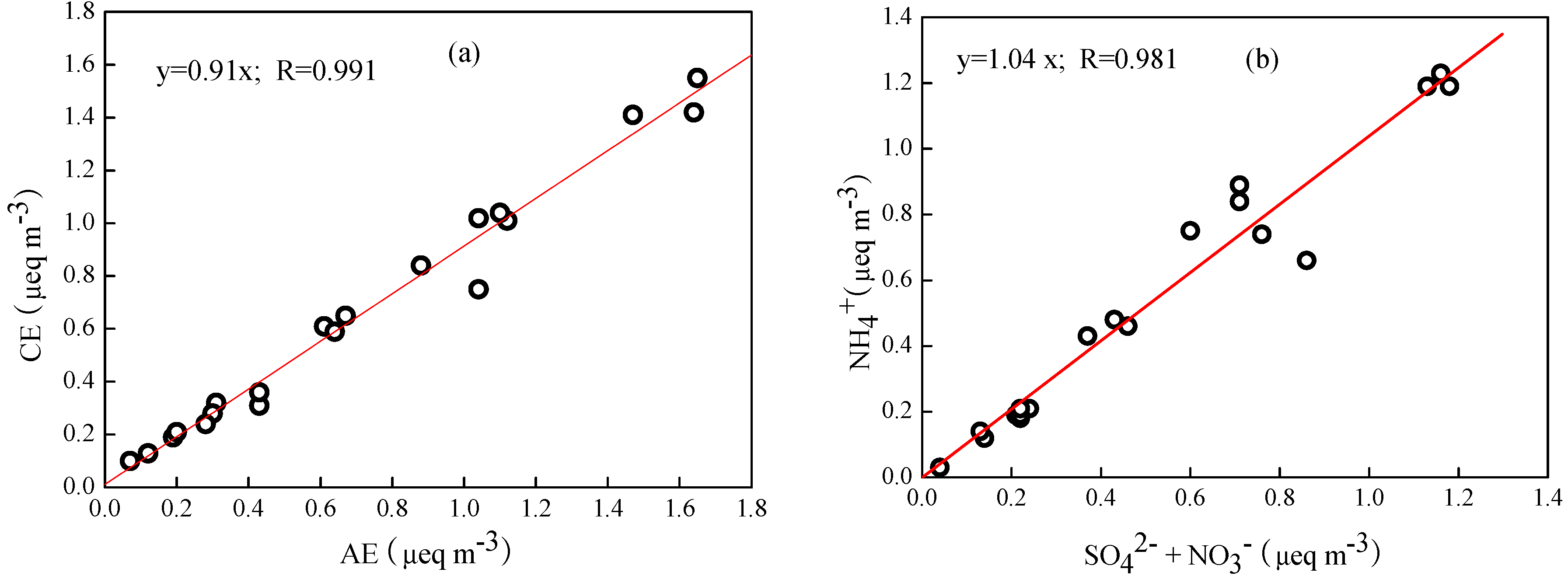
2.3. Quality Control

The fresh quartz filters were pre-heated at 450 °C in a muffle furnace for 6 h to remove any volatile components before sampling. Furthermore, after collection, the samples were sealed in clean plastic bags, and were stored in a freezer at −18 °C before chemical analysis to minimize the evaporation of volatile components. Before and after sampling, the Teflon filters in the first channel were weighed after being equilibrated for 24 h. The artifacts during the sampling and analysis were estimated by a field blank filter.

2.4. Measurements of Aerosol Optical and Meteorological Parameters

BC mass concentration, σsc and meteorological data were measured on the roof of the Physics Building about 30 m above the ground in Peking University, which is about 1 km away from the sampling sites of Tsinghua University. An automatic weather station (Vaisala Ltd., Helsinki, Finland) was used to record wind speed (WS), wind direction, relative humidity (RH), temperature (Temp), and visibility (VR).
σsc was monitored using a single wavelength (525 nm) integrating Nephelometer (M9003, Ecotech, Melbourne, VIC, Australia). This instrument drew ambient air through a heated inlet tube to maintain RH in the Nephelometer chamber below 60%. The scattering intensity over angles from 7° to 170° was measured and integrated to yield the scattering coefficient. Zero calibration was performed every two days with particle-free air to subtract the Rayleigh scattering, while span calibration was carried out every month using R-134 gas.
BC mass concentration was measured with an Aethalometer (AE-16, Magee Scientific, Berkeley, CA, USA). The principle of this instrument to calculate the BC concentration is based on the attenuation of an incident beam at a wavelength of 800 nm caused by the particles loaded in the quartz filter. No size-selective inlet was used for both the nephelometer and aethalometer. Considering the negligible contribution of coarse particles to light extinction, the measured σsc can be approximately attributed to the PM2.5.

2.5. Data Analysis

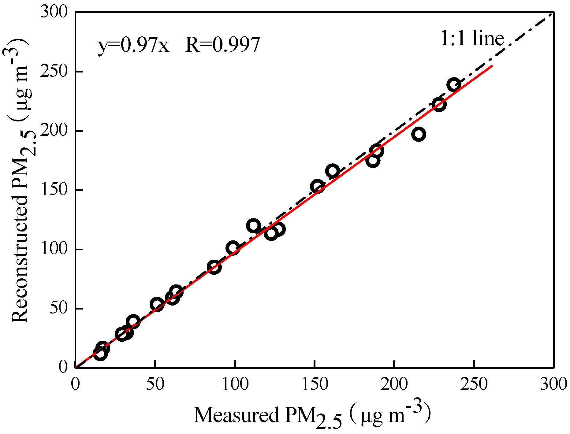
2.5.1. Reconstruction of PM2.5 Mass

PM2.5 components can be grouped as follows: secondary inorganic aerosols (SNA), OM, EC, fine soil (FS), and chloride salt (CS). SNA is the sum of SO42−, NO3, and NH4+, and OM is derived from multiplying OC concentrations by a factor of 1.6 to account for unmeasured atoms according to Xing et al. [23], which demonstrated that the calculated OM/OC mass ratio in summer was relatively high (1.75 ± 0.13) and in winter was lower (1.59 ± 0.18) in PM2.5 collected from 14 Chinese cities. Beijing is far from the coastal oceans, and sea salt is not transported to Beijing, thus it has a minor contribution to PM2.5 in Beijing. The CS was considered instead of sea salt, and estimated by summing concentrations of Cl, K+, and Na+ according to Zhang et al. [12].
The concentrations of FS are often estimated by assuming the oxides of the elements mainly associated with soil (Al2O3, SiO2, K2O, CaO, FeO, Fe2O3, and TiO2), which is calculated as follows [24]:
[FS] = 2.20[Al] + 2.49[Si] + 1.63[Ca] + 2.42[Fe] + 1.94[Ti]

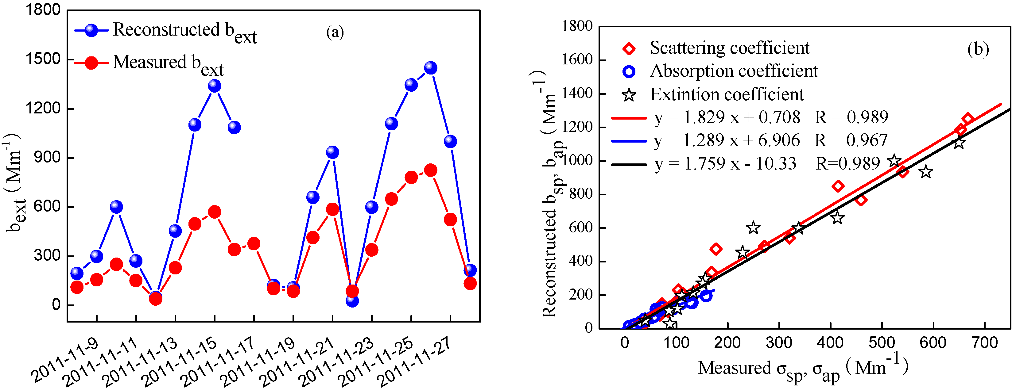
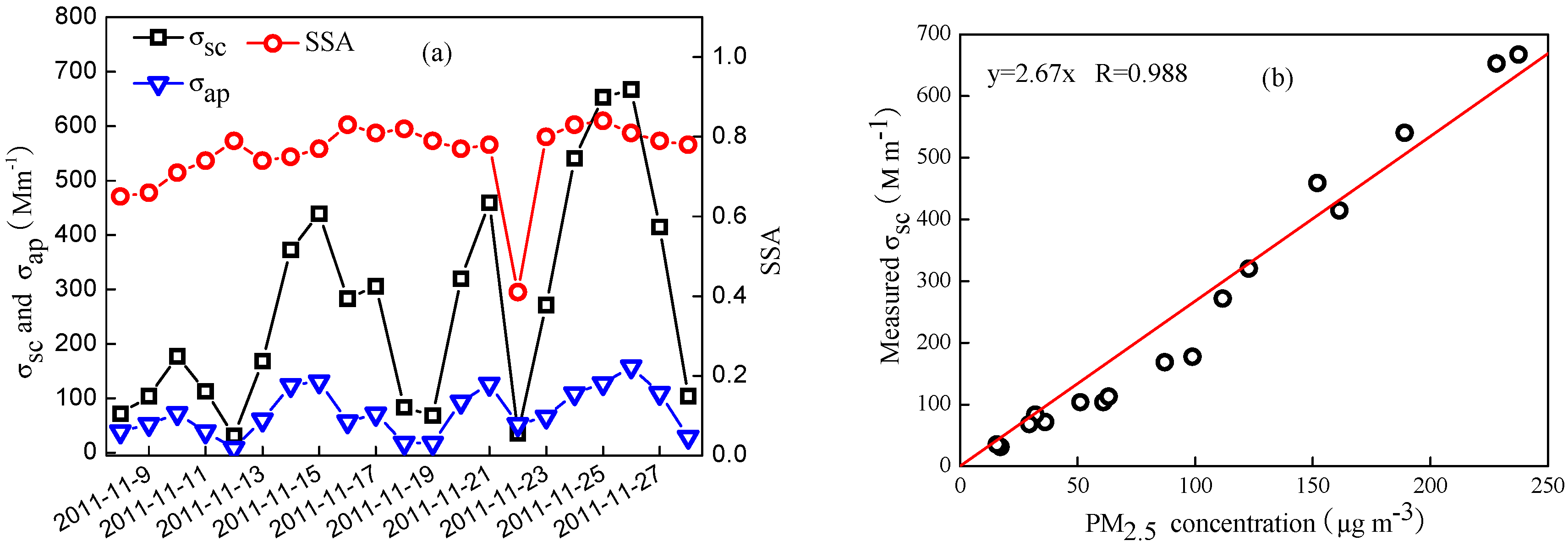
2.5.2. Reconstruction of the Light Extinction Coefficient

According to the revised IMPROVE algorithm, the reconstructed bext is shown from the following equation assuming an externally mixed aerosol [20]:
b e x t = b s p + b a p + b a g + b s g         2.2 × f s ( R H ) × [ S m a l l ( N H 4 ) 2 S O 4 ] + 4.8 × f L ( R H ) × [ L arg e ( N H 4 ) 2 S O 4 ]            + 2.4 × f s ( R H ) × [ S m a l l N H 4 N O 3 ] + 5.1 × f L ( R H ) × [ L arg e N H 4 N O 3 ]            + 2.8 × [ S m a l l O M ] + 6.1 × [ L arg e O M ]            + 10 × [ E C ] + 1 × [ F i n e S o i l ] + 1.7 × f s s ( R H ) × [ S e a S a l t ] + 0.6 × [ P M 2.5 ~ 10 ]            + 0.33 × [ N O 2 ( p p b ) ] + R a y l e i g h S c a t t e r i n g
The algorithm divides the concentrations of SO42−, NO3, and OM into small and large-sized fractions. The size modes are described by log-normal mass size distributions with geometric mean diameter and geometric standard deviations. The fraction of a component in the large- or small-sized mode was estimated by an empirical approach [20]. The apportionment of the total concentrations of (NH4)2SO4 into the concentrations of the small and large size fraction in PM2.5 is accomplished using the following equations:
[ L arg e ( N H 4 ) 2 S O 4 ] = [ T o t a l ( N H 4 ) 2 S O 4 ] 20 μ g . m 3 × [ T o t a l ( N H 4 ) 2 S O 4 ] , f o r [ T o t a l ( N H 4 ) 2 S O 4 ] < 20 μ g . m 3
[ L arg e ( N H 4 ) 2 S O 4 ] = [ T o t a l ( N H 4 ) 2 S O 4 ] , f o r [ T o t a l ( N H 4 ) 2 S O 4 ] > 20 μ g . m 3
[ S m a l l ( N H 4 ) 2 S O 4 ] = [ T o t a l ( N H 4 ) 2 S O 4 ] [ L arg e ( N H 4 ) 2 S O 4 ]
Similar equations are used to apportion total NH4NO3 and total OM concentrations into small and large size fractions. The water growth adjustment term fs(RH), fL(RH) for small and large size distribution of (NH4)2SO4 and NH4NO3, and fss(RH) for sea salt are used according to the water growth curves provided by Pitchford et al. [20].
According to the revised IMPROVE method, SO42− and NO3 are assumed to be fully neutralized by NH4+ in the forms of (NH4)2SO4 and NH4NO3, respectively. Therefore, (NH4)2SO4 mass is estimated by the SO42− mass multiplied by a factor of 1.38, and the NH4NO3 mass is estimated by the NO3 mass multiplied by a factor of 1.29.
In order to compare with the reconstructed bext calculated using Mie theory at 550 nm, σsc measured at 525 nm with the integrating nephelometer should be converted to that at 550 nm according to the method by Jung et al. [16].
σ s c ( 550 n m ) = σ s c ( 525 n m ) * ( λ ( 550 n m ) λ ( 525 n m ) ) α
where α is the scattering Angström exponent, an average α value of 1.18 determined in Beijing during the summer of 2012 by Tian et al. [18] was used in the present study.
σab at 550 nm was calculated based on BC concentration following the equation:
σab = K × [BC]
where K is the conversion factor, which was set to 8.1 m2∙g−1 in this study according to a previous study [25].
The single scattering albedo (SSA) is defined as the ratio of the aerosol scattering coefficient to the extinction coefficient at a known wavelength, as derived from the formula:
S S A = σ s c σ s c + σ a b

3. Results and Discussion

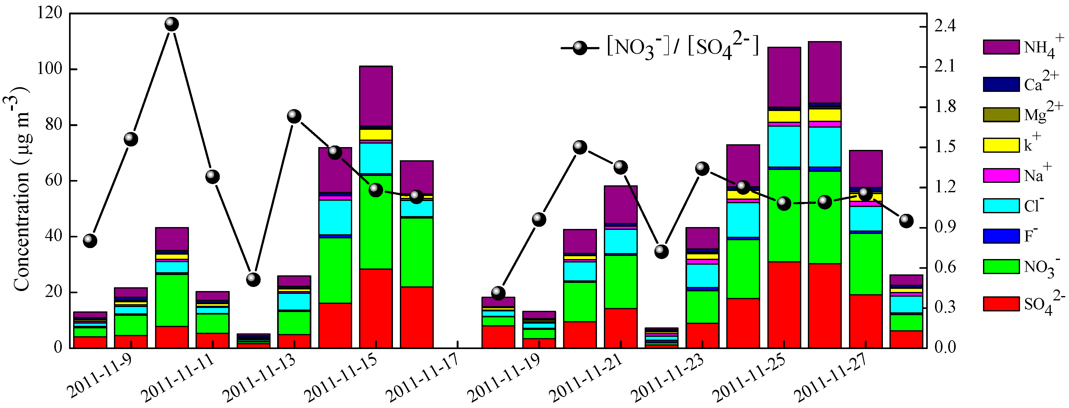
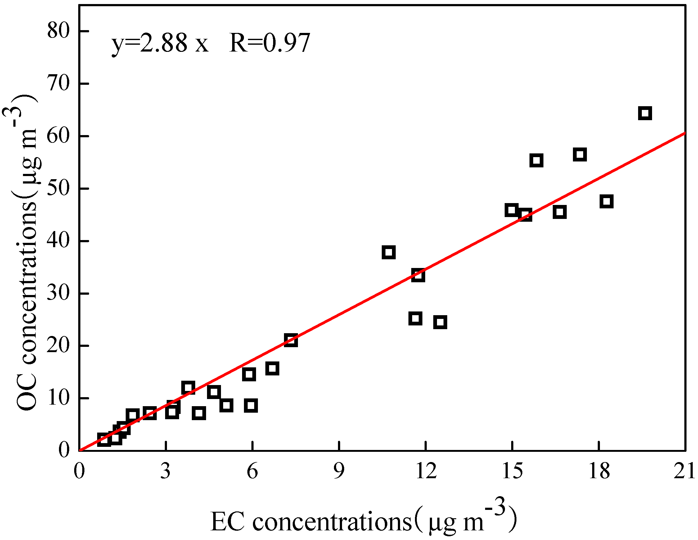
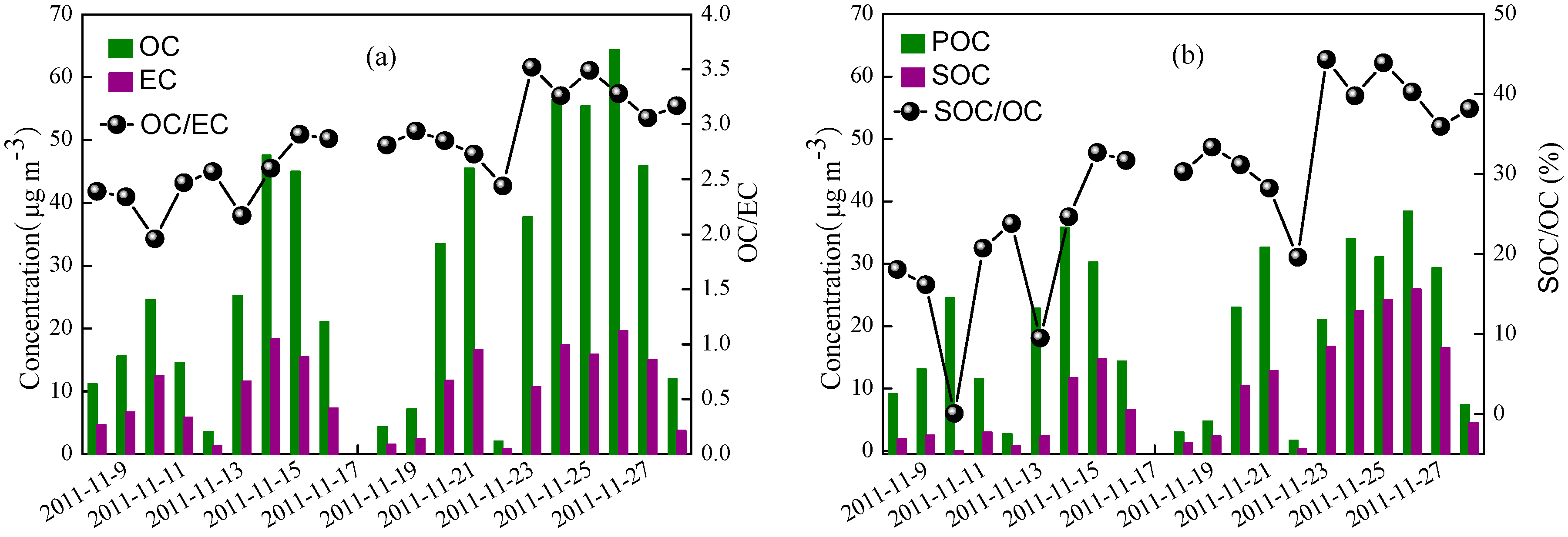
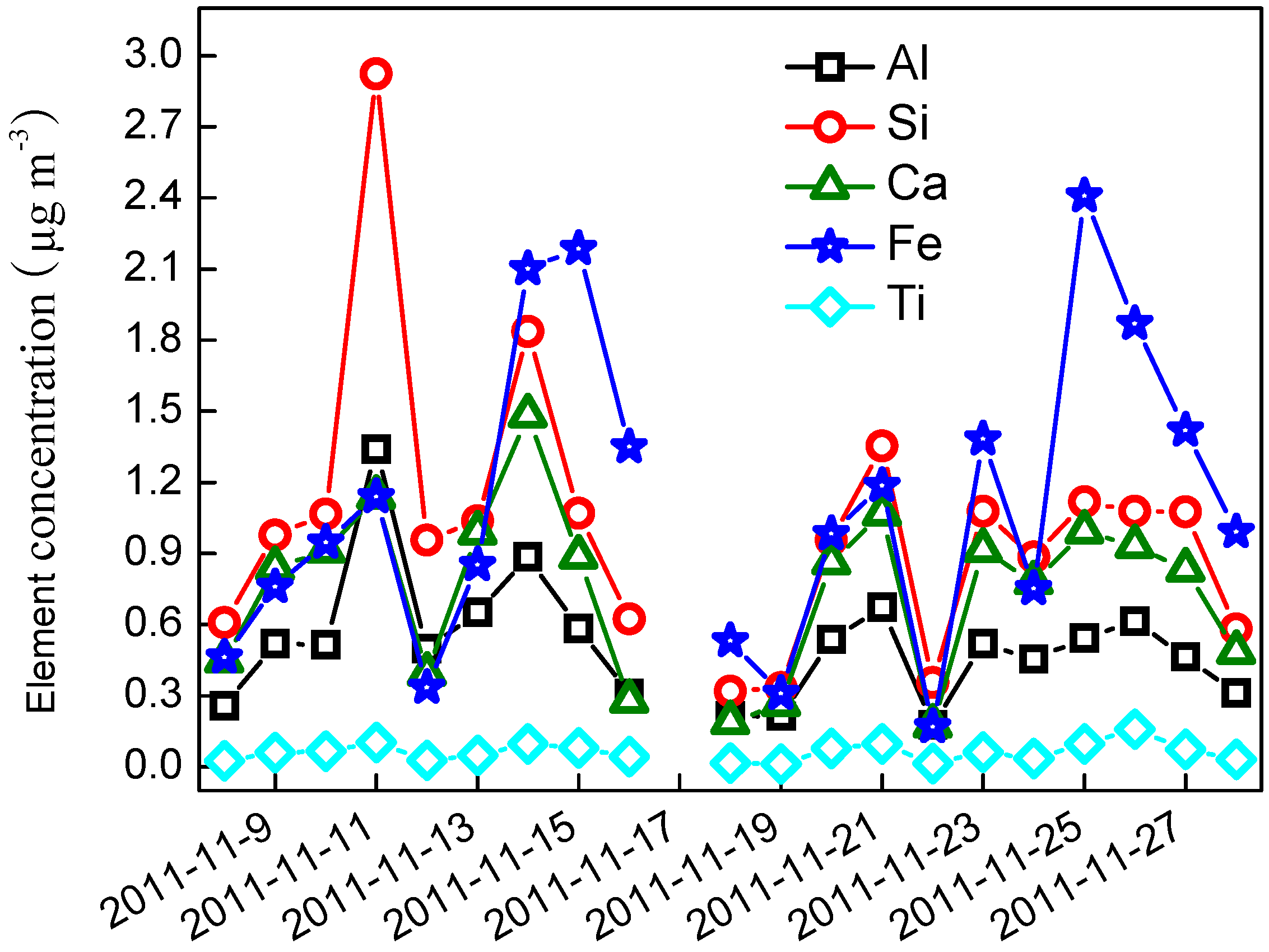
3.1. PM2.5 Chemical Compositions

The time series of daily PM2.5 mass concentrations and the meteorological parameters, including RH, temperature, and WS are shown in Figure 1. The mass concentrations of PM2.5 ranged from15.6–237.5 μg∙m−3 and averaged 111.2 ± 73.4 μg∙m−3. Compared with other studies conducted in urban Beijing, the average PM2.5 concentration in this study was lower than that measured during autumn of 2006 (194.2 μg∙m−3) [26] and 2009 (135 μg∙m−3) [12], while comparable with that observed during the same season in 2005 (115.0 μg∙m−3) and 2012 (106.9 μg∙m−3) [27]. There were sixty percent of days with daily PM2.5 mass concentration exceeding the China Ambient Air Quality Standards(75 μg∙m−3). The highest PM2.5 mass concentration occurred on 26 November, which was associated with the high relative humidity and low wind speed.
Figure 1. Daily variations of PM2.5 mass concentration and meteorological parameters.
Atmosphere 06 00164 g001
The temporal variations of nine water-soluble inorganic ions (WSIIs) are presented in Figure 2. The average concentration of total nine ions was 46.9 ± 33.8 μg∙m−3, accounting for 41.5% of PM2.5 mass concentration. NO3 was the most abundant species in WSIIs with an average concentration of 14.7 ± 11.2 μg∙m−3, followed by SO42− (12.2 ± 9.63 μg∙m−3), NH4+ (9.13 ± 7.26 μg∙m−3), and Cl (6.62 ± 4.62 μg∙m−3), accounting for 28.9%, 25.6%, 17.7%, and 14.6% of WSIIs, respectively. The rest of K+ (1.66 ± 1.41 μg∙m−3), Na+ (0.95 ± 0.52 μg∙m−3), Ca2+ (0.81 ± 0.32 μg∙m−3),F (0.61 ± 0.34 μg∙m−3), and Mg2+ (0.25 ± 0.18 μg∙m−3) each had a minor contribution to the WSIIs, totally accounting for 13.2% of WSIIs. SNA typically constituted 33.5%–87.1% of the total WSIIs and 15.3%–46.0% of PM2.5, respectively.
Figure 2. Daily variations of water-soluble ions and [NO3]/[SO42−] ratios.
Atmosphere 06 00164 g002
NO3 and SO42− are mainly formed by atmospheric reactions of precursor gases such as NOx and SO2. Generally, SO2 emits from coal combustion, while NOx is the result of any type of combustion such as coal-fired power plants and automobiles. The mass ratio [NO3]/[SO42−] has been used to identify the influence of the stationary and mobile sources of sulfur and nitrogen [28]. The [NO3]/[SO42−] ratio ranged from 0.41–2.42, with an average value of 1.19. It was higher than that of values (around 0.68) measured in Beijing from 2001–2006 [26,29,30,31], but rather more comparable to those observed in recent years [12]. As illustrated in Figure 2, the ratio was usually lower during weekend days (12, 18–19 November) than on workdays, indicating that the higher [NO3]/[SO42−] ratio in the present study was probably associated with the rapid increase of motor vehicles in recent years. According to the statistics from the China Vehicle Emission Control Annual Report in 2013, the amount of vehicles reached 5 million in Beijing by 2012, which was an increase of about three times compared with the amount of vehicles in 2001 [32].
Previous study showed that Cl might be derived from coal combustion when the Cl/Na+ equivalent concentration ratios were larger than the mean ratio (1.17) for sea water. The ratios of Cl/Na+ were in the range of 1.6–11.6 with a mean value of 6.63 during the study period, implying that Cl may be originated from coal combustion rather than sea spray [12].
The equivalent molar ratio of total cations to total anions (CE/AE) ranged from 0.71–1.40, with an average value of 0.95 ± 0.14 during the study period. Figure 3 illustrates the scatter plots of the sum of cations versus anions. Results showed that the slope was slightly lower than 1, implying that the fine particles collected in the study period were weakly acidic. Moreover, the ratios of [NH4+]/[SO42− + NO3] were close to 1, demonstrating that SO42− and NO3 were fully neutralized by NH3. Therefore, the dominant chemical form of SO42− was (NH4)2SO4 rather than NH4HSO4, which can be estimated by the SO42− mass concentration multiplied by a factor of 1.38, while NO3 existed as NH4NO3, and can be estimated by the NO3 mass concentration multiplied by a factor of 1.29.
Figure 3. Relationships of equivalent concentrations of cations versus anions (a) and [NH4+] versus [SO42− + NO3] (b).
Atmosphere 06 00164 g003
As illustrated in Figure 4, OC varied from 2.1 to 64.3 μg∙m−3, averaging 27.5 ± 19.9 μg∙m−3, while EC ranged from 0.86 to 19.6 μg∙m−3, averaging 9.62 ± 6.24 μg∙m−3. The contribution of OC and EC to PM2.5 were 24.5% and 8.96%, respectively. Such levels of OC and EC were close to those observed in the same season in recent years [10,26,30,33], whereas lower than those measured ten years ago [29,34].
Figure 4. Variations of OC, EC, and OC/EC (a) as well as primary organic carbon (POC), secondary organic carbon (SOC), and SOC/OC (b).
Atmosphere 06 00164 g004
The relationships between OC and EC can be used to identify the origins of carbonaceous particles [35,36]. As shown in Figure 5, strong correlations between OC and EC were observed with a correlation coefficient of 0.97, indicating that OC and EC were likely derived from the same major primary sources during the campaigns. On the other hand, the OC/EC ratios did not vary distinctly during the study period, especially during the space heating days. The ratios ranged from 1.96–3.52, averaging 2.79, and were very close to the value of 2.7 from coal combustion suggested by Watson et al. [37]. This pointed to the fact that OC and EC likely originated mainly from coal combustions. Furthermore, the mean OC/EC ratio was higher than 2, indicating that SOC might be present during the study period [38].
Figure 5. Relationships of OC and EC concentrations.
Atmosphere 06 00164 g005
The method of EC-tracer has been widely used to estimate the SOC concentration since it was first introduced by Castro et al. [9,39]. This approach suggested that samples having the lowest OC/EC ratio contained almost exclusively POC. Then, the concentration of SOC can be estimated by the following formula:
POC = EC × (OC/EC)min
SOC = OC – POC
where (OC/EC)min was the value of the lowest OC/EC ratio. Based on the (OC/EC)min of 1.63, the SOC concentrations varied from 0.02–25.9 μg∙m−3 with an average value of 9.03 μg∙m−3. As illustrated in Figure 4, it is interesting to note that the concentrations of SOC were still high with low temperature during the study period except on 10, 12 and 22 November. This may be caused by the combination of the high precursor emission due to the largely increased coal combustion for residential heating and low wind speed (averaging 0.79 m∙s−1), which was favorable for the pollutants accumulation and formation of secondary organic aerosol. The low temperature was not favorable for the gas to particle conversion, whereas the frequent inversion conditions were likely favorable for the formation of SOC [40].
Daily variations of crustal elements are shown in Figure 6. Five crustal elements have a similar variation as the PM2.5 mass concentrations. Their concentrations varied significantly from day to day. The average concentration for Al, Si, Ca, Fe, and Ti was 0.51 ± 0.26, 1.01 ± 0.58, 0.74 ± 0.36, 1.10 ± 0.64, and 0.06 ± 0.03 μg∙m−3, respectively. Increasing wind speed could be expected to increase the concentrations of crustal elements, but the concentration of the five elements had a weak correlation with the wind speed (R < 0.4) in the present study. However, when the wind speed exceeded 1.5 m∙s−1 (11 and 18 November), the concentrations of crustal elements were higher than those on any other day. The FS mass concentration was estimated by summing the above five crustal elements plus oxygen for the normal oxides as Equation (1). The average mass concentrations of FS were 7.66 ± 3.62 μg∙m−3, ranging from 1.99–15.1 μg∙m−3, and accounting for 9.42% of PM2.5.
Figure 6. Time series of crustal elements concentration.
Atmosphere 06 00164 g006

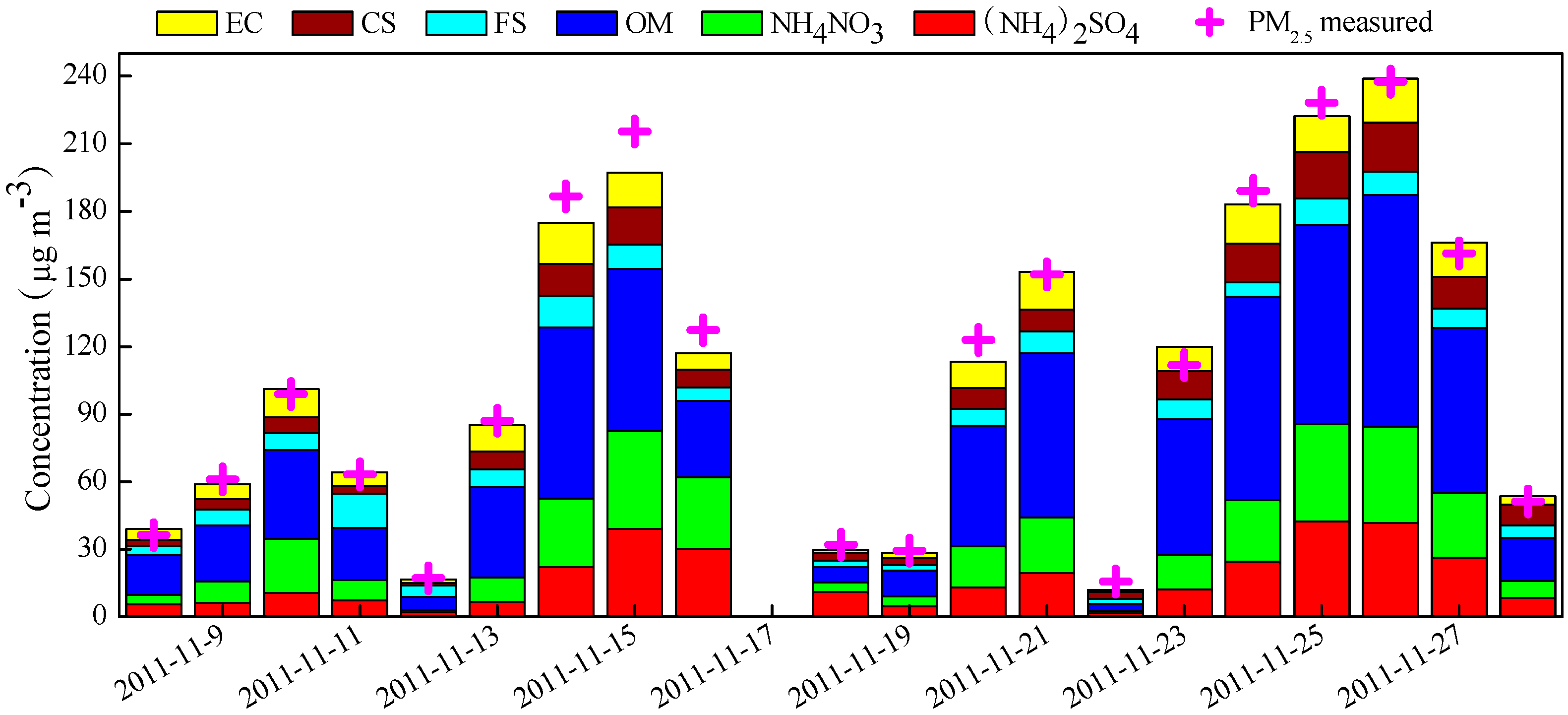
3.2. PM2.5 Mass Balance

The reconstructed PM2.5 mass concentrations were close to the measured ones with strong correlation (Figure 7), indicating that the reconstruction of PM2.5 could be reasonable. Nevertheless, a few biases were observed in the reconstructed PM2.5 mass. Water absorption of the water-soluble components may lead to positive biases and overestimate the PM2.5 mass, while the volatilization of NH4NO3 and volatile organic matter may result in negative biases. Moreover, the conversion used to estimate OM from OC also caused an uncertainty in calculating the PM2.5 mass.
Figure 7. Scatter plots of measured and reconstructed PM2.5 mass concentrations.
Atmosphere 06 00164 g007
Figure 8 presents the reconstructed chemical compositions in PM2.5. On average, the fractions of major chemical compositions followed the order of OM > NH4NO3 > (NH4)2SO4 > FS, CS, and EC. OM was the most abundant component in PM2.5 (averaging 45.8 ± 31.7 μg∙m−3), accounting for 39.4% of PM2.5. The contribution of FS (averaging 7.66 ± 3.62 μg∙m−3), CS (averaging 9.47 ± 6.24 μg∙m−3), and EC (averaging 9.97 ± 6.28 μg∙m−3) to PM2.5 was similar, each approximated to 9%. The percentage of SNA (30.2%) was much higher than the three species of FS, CS, and EC, but slightly lower than that of OM. The percentages of (NH4)2SO4 and NH4NO3 (averaging 16.7 ± 13.2 and 19.0 ± 14.4 μg∙m−3, respectively) were 14.9% and 15.4%, respectively. Compared with the results determined over the same period in earlier years [11], it is noted that the percentage of SNA in our study decreased by 3%–10% compared with that measured during 2003–2007, while the OM fraction rose about 5%.
Figure 8. Daily variations of the reconstructed chemical composition in PM2.5.
Atmosphere 06 00164 g008

3.3. Analysis of Aerosol Optical Properties

The time series of daily averaged optical properties including σsc, σap, and SSA are shown in Figure 9. Daily σsc ranged from 31.1–667 Mm−1, with a mean value of 270 ± 200 Mm−1, while σap was in the range of 8.24–158.0 Mm−1, with a mean value of 74.3 ± 43.4 Mm−1. The mean σsc value was considerable lower than that measured in urban Beijing in 2009 and during 2005–2006 [41,42], but higher than that obtained at a suburban site (Changping) and rural site (Shangdianzi) [15]. Compared with the results mentioned above, the mean σap value was lower than that measured in 2009 as well, but higher than that during 2005–2006. The increased σap in recent years is likely attributable to the rapid increase of vehicle pollution, since vehicular exhaust was one of the primary factors affecting aerosol absorption. The mean value of SSA was 0.76, which was comparable with the results determined in Beijing during 2005–2006 [42] and in 2009 [41].
MSE is an important parameter for estimating radiative forcing of aerosols and chemical extinction budgets for visibility impairment. Generally, there are two methods to estimate MSE, i.e., measurement method and multilinear regression method [43]. MSE was defined as the ratio of measured σsc to aerosol mass concentration according to the measurement method. One alternative method can also be used by regression of the measured σsc against aerosol mass concentration. Since the RH in the nephelometer was maintained below 60% and the PM2.5 mass concentrations were measured at RH of 40%, those days with RH below 50% were selected for regressing to minimize the impact of particle hygroscopic growth on σsc. According to the measurement method, daily MSE varied from 1.70–3.02 m2∙g−1, with a mean value of 2.32 ± 0.44 m2∙g−1. It is noted that a strong correlation between the measured σsc and PM2.5 mass concentration was observed with a high correlation coefficient of 0.988 (Figure 9). The slope was 2.67 from a linear regression, which was slightly higher than the value obtained by the measurement method, also found by Titos et al. [43]. Compared to that measured in urban Beijing by Zhao et al., and Jing et al. [41], the relative lower MSE in our study was likely related to the heavily polluted events.
Figure 9. The time series of daily averaged aerosol optical properties (a) and relationship between the measured σsc and PM2.5 concentration (b).
Atmosphere 06 00164 g009

3.4. Chemical Apportionment of the Aerosol Optical Parameters

In order to appoint the contribution to the visibility impairment, bext was reconstructed based on the chemical compositions of aerosol. In the present study, the extinction effect by fine particles was studied, while the contributions of gases were excluded because they only accounted for a small fraction (about 2%–4%) of bext [44]. The impact of sea salt on bext was ignored since Beijing is about 150 km away from the East China’s coastal oceans. Moreover, the contribution of coarse mass to bext was not included because of lack of the concentrations of coarse matter. Then, the revised IMPROVE formula of Equation (2) was modified as follows:
b e x t = 2.2 × f s ( R H ) × [ S m a l l ( N H 4 ) 2 S O 4 ] + 4.8 × f L ( R H ) × [ L arg e ( N H 4 ) 2 S O 4 ]            + 2.4 × f s ( R H ) × [ S m a l l N H 4 N O 3 ] + 5.1 × f L ( R H ) × [ L arg e N H 4 N O 3 ]            + 2.8 × [ S m a l l O M ] + 6.1 × [ L arg e O M ]            + 10 × [ E C ] + 1 × [ F i n e S o i l ]
The measured and reconstructed bext are illustrated in Figure 10. It is found that the measured bext were considerably lower than the reconstructed value, especially during the heavily pollution levels. The deviation varied from 18.1%–140%, with an average value of about 70%. Jung et al. [45] also found that the bext was overestimated by 36.7% based on the revised IMPROVE algorithm. However, a few other studies using the IMPROVE formula found that there existed a good correlation between the measured and reconstructed bext, and the slopes were close to 1.0 in Shanghai [19] and Guangzhou [4]. Compared to the results conducted in Shanghai, a lower MAE (7.7) was used to calculate bap. If the same value of 7.7 was used in the present study, the biases would decrease by 8%. Additionally, the MSE used to calculate bext in Guangzhou was much higher than the value in the present study. Thus, it can be deduced that a lower MSE than the value adopted according to the revised IMPROVE algorithm in the present study should be used to reconstruct bext, which may result in a reconstructed bext approximately equal to the measured bext. Although more locally-derived MSE and MAE were necessary for effectively reconstructing the bext, we did not obtain these values in the present study due to lack of the amount of in situ and sampling data.
Figure 10. The temporal variations of measured and reconstructed bext (a) and the correlation between measured and reconstructed optical parameters (b).
Atmosphere 06 00164 g010
Although the reconstructed bext was higher than that measured one, both were correlated well (R = 0.989), so did bsp and bap (Figure 11). Therefore, the relative contribution of each chemical composition to bext can also be analyzed by the modified IMPROVE algorithm. As shown in Figure 11, OM, (NH4)2SO4, NH4NO3 and EC were the dominant contributors, accounting for 97.7% of bext together, while the contribution of FS was small, accounting for only 2.3% of bext. On average, OM was the largest contributor to the bext, accounting for 44.7% of bext, while SNA accounted for 34.4% of bext. (NH4)2SO4 and NH4NO3 contributed 16.4% and 18.0% of bext, respectively. Our results were different from those determined in Beijing in previous studies conducted in summer [16,18,46], which showed that (NH4)2SO4 and NH4NO3 were the largest contributor to the bext.
Figure 11. Relative contributions of each chemical composition in PM2.5 to bext.
Atmosphere 06 00164 g011

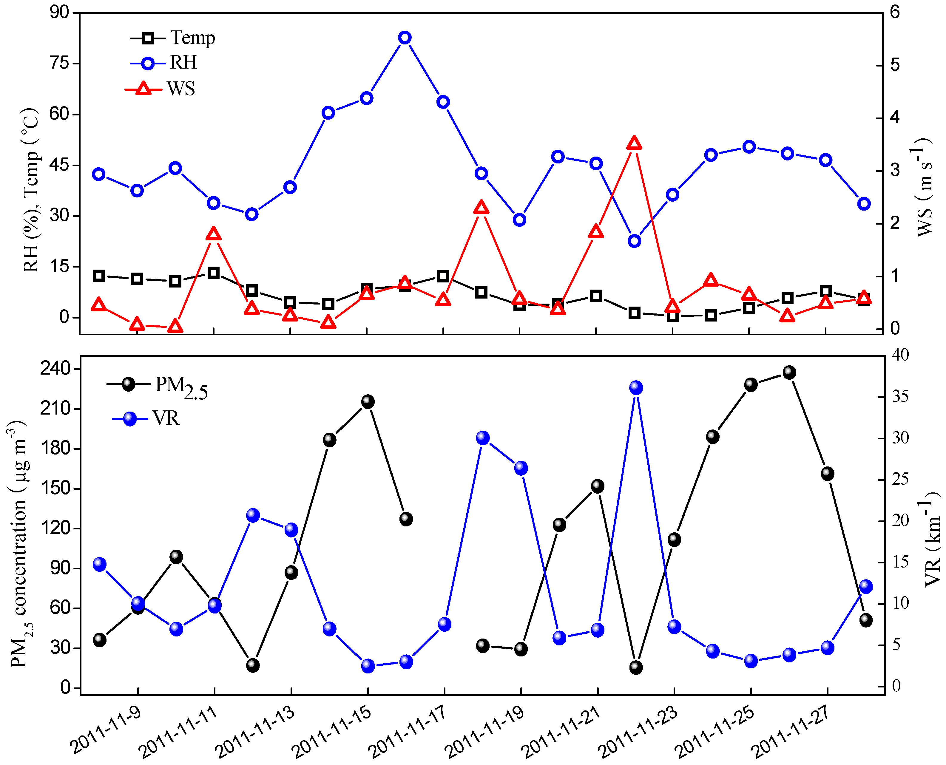
3.5. Typical Pollution Episodes

As shown in Figure 1, four obvious pollution episodes were observed during the campaign, with the visibility deteriorating to less than 10 km. They were observed on 9–11 November, 14–17 November, 20 and 21 November, and 23–27 November. Obviously, in the first pollution period, pollutants accumulated gradually from 8–10 November, with daily PM2.5 mass concentration increasing from 36.3–98.8 μg∙m−3, and then decreasing dramatically to 17.1 μg∙m−3. All the chemical components increased with PM2.5 mass, especially for NO3, which increased by six times compared with the value on 8 November. Furthermore, it can be found that during the pollution accumulation period, the wind speed was less than 0.5 m∙s−1. On 11 November, strong wind was favorable for dispersion of the pollutants and accumulation of the crustal material. Moreover, 12 November was weekend, and the reduction of vehicles may also contribute to the lower concentration of PM2.5. From an extinction perspective, in the first pollution stage, σsc increased from 71.6–177.2 Mm−1, while σap varied little, implying that the visibility degradation was mainly caused by the rapid increase of SNA.
In the second pollution period from 12–19 November, daily PM2.5 mass concentration increased from 17.1–215.5 μg∙m−3, with the maximum value occurring on 15 November, and then plunging to 32.0 μg∙m−3 within three days. As illustrated in Figure 1, it can be found that the wind speeds were very low from 12–15 November, and in favor of the accumulation of the pollutants. On the other hand, the RH increased from 30% to 82%, which was favorable for the formation of SNA. Residential heating starting in the middle of November might be the primary reason for the heavier pollution in the second stage. As shown in Figure 2, the concentration of Cl on 13 November had a dramatic increase compared with the previous days, approximately to 10 times higher than that on 12 November. Chloride may be essentially contributed by coal combustion in Beijing during the heating season. Thus, the high PM2.5 mass concentration was mainly associated with coal combustion. In fact, the concentrations of OC and EC during 13–27 November were much higher than those before 12 November. The sharp increase of OC and EC also verified the influence of coal combustion on the increase of PM2.5 mass concentration. Unlike the first pollution stage, σap on the most heavy pollution day (15 November) was about 15 times higher than that on the clean days. Meanwhile, σsc rose from 31.0–439.2 Mm−1, with a similar growth rate as σap. As shown in Figure 11, during the second pollution episode, the contribution of OM and EC to bext decreased from 54.2% and 25.6% to 32.7% and 11.5% as the pollutants accumulated, respectively, while the contribution of SNA to bext increased from 18.3%–54.8% on the accumulation period. On 16 November, although the mass concentration of PM2.5 reduced by 40%, the visibility was still less than 3 km, which was ascribed to the largest contribution of SNA to bext. As presented in Figure 11, the contribution of SNA reached up to 73.7% whereas that of OM and EC decreased to 26.7% to bext. The PM2.5 mass concentration had a significant decrease on 18 November due to rain and strong wind (Figure 1).
Based on the analysis of a typical pollution episode, it can be concluded that the secondary formation of aerosol was more important than the carbonaceous pollution for the haze formation in Beijing. In the other two pollution periods, a similar trend of the chemical composition to that during the second pollution stage was observed. In general, the pollution accumulation was in accordance with the increase of the SNA, OC and EC concentrations under stable weather conditions until arrival of strong wind.

4. Conclusions

During the heating period from 8–28 November 2011, aerosol optical properties as well as chemical compositions were investigated simultaneously in Beijing. Daily PM2.5 mass concentration varied from 15.6–237.5 μg∙m−3 and presented a mean value of 111.2 ± 73.4 μg∙m−3. Among the chemical components in PM2.5, NO3 was the most abundant species in WSIIs with an average concentration of 14.7 ± 11.2 μg∙m−3, followed by SO42−, NH4+, and Cl, accounting for 28.9%, 25.6%, 17.7%, and 14.6% of WSIIs, respectively. The rest of K+, Na+, Ca2+, F, and Mg2+ have a minor contribution to the WSIIs, accounting for 13.2% of WSIIs together.
The mean σsc, σap and SSA values at 550 nm were 270 ± 200 Mm−1, 74.3 ± 43.4 Mm−1 and 0.76 during the entire observation period, respectively. Both of the σsc and σap increased significantly during the pollution accumulation episode. The bext were estimated by the revised IMPROVE formula based on the chemical compositions of PM2.5. Compared with the measured σsc and σap, the reconstructed bext was overestimated, but had a strong correlation with a high correlation coefficient of 0.989. OM was the largest contributor, accounting for 44.7% of bext, followed by NH4NO3, (NH4)2SO4, with minor contribution from soil dust (2.3%).
Pollution episodes in Beijing were strongly influenced by both emissions and meteorological conditions. Pollutant was accumulated in calm or weak winds while diffused under strong wind conditions. Additionally, the coal combustion for residential heating was another major reason for the heavy pollution during the sampling period. Four typical pollution episodes during the study period were observed, it was found that NH4NO3 and (NH4)2SO4 were the largest contributor to the bext rather than carbonaceous components during the pollution accumulation episodes, implying that the secondary inorganic pollutants were more important than the carbonaceous pollution for heavy pollution formation. Therefore, the reduction of their precursors such as SO2, NOx and NH3 could effectively improve the visibility in Beijing.

Acknowledgments

This study was supported by the National Natural Science Foundation of China projects (41075093, 41275121 and 41375123), the “Strategic Priority Research Program” of the Chinese Academy of Sciences (KJZD-EW-TZ-G06-04), the Ministry of Environmental Protection of China (201209007), State Environmental Protection Key Laboratory of Sources and Control of Air Pollution Complex (SCAPC201310), Jiangsu Key Laboratory of Atmospheric Environment Monitoring and Pollution Control of Nanjing University of Information Science and Technology, and Jiangsu Province Innovation Platform for Superiority Subject of Environmental Science and Engineering (KHK1201). The authors thank Lian-fang Wei, Jin-lu Dong, and Rong Zhang for their contributions to the field and laboratory work.

Author Contributions

The work was completed with collaboration between all the authors. The corresponding author designed the research theme, organized the PM2.5 sampling with Xinghua Li, checked the experimental results, and designed the manuscript with Huanbo Wang. Huanbo Wang analyzed the data, interpreted the results and wrote the manuscript. Xinghua Li was in charge of PM2.5 sampling and collected all relevant data, and Chengcai Li was in charge of observation of optical parameters. Junji Cao was in charge of inorganic elements analysis. Yongliang Ma and Kebin He provided analyses of water-soluble ions and OC/EC. Guangming Shi was involved in relevant data interpretation and discussion.

Conflicts of Interest

The authors declare no conflict of interest.

References

  1. Wang, Q.Y.; Cao, J.J.; Tao, J.; Li, N.; Su, X.O.; Chen, L.W.A.; Wang, P.; Shen, Z.X.; Liu, S.X.; Dai, W.T. Long-term trends in visibility and at Chengdu, China. PLoS One 2013. [Google Scholar] [CrossRef]
  2. Zhang, X.Y.; Wang, Y.Q.; Niu, T.; Zhang, X.C.; Gong, S.L.; Zhang, Y.M.; Sun, J.Y. Atmospheric aerosol compositions in China: Spatial/temporal variability, chemical signature, regional haze distribution and comparisons with global aerosols. Atmos. Chem. Phys. 2012, 12, 779–799. [Google Scholar] [CrossRef]
  3. Shen, G.F.; Xue, M.; Yuan, S.Y.; Zhang, J.; Zhao, Q.Y.; Li, B.; Wu, H.S.; Ding, A.J. Chemical compositions and reconstructed light extinction coefficients of particulate matter in a mega-city. In the western Yangtze River Delta, China. Atmos. Environ. 2014, 83, 14–20. [Google Scholar] [CrossRef]
  4. Tao, J.; Zhang, L.M.; Ho, K.F.; Zhang, R.J.; Lin, Z.J.; Zhang, Z.S.; Lin, M.; Cao, J.J.; Liu, S.X.; Wang, G.H. Impact of PM2.5 chemical compositions on aerosol light scattering in Guangzhou—The largest megacity in south China. Atmos. Res. 2014, 135, 48–58. [Google Scholar] [CrossRef]
  5. Chen, J.; Qiu, S.S.; Shang, J.; Wilfrid, O.M.F.; Liu, X.G.; Tian, H.Z.; Boman, J. Impact of relative humidity and water soluble constituents of PM2.5 on visibility impairment in Beijing, China. Aerosol Air Qual. Res. 2014, 14, 260–268. [Google Scholar]
  6. Ramanathan, V.; Feng, Y. Air pollution, greenhouse gases and climate change: Global and regional perspectives. Atmos. Environ. 2009, 43, 37–50. [Google Scholar] [CrossRef]
  7. Ma, X.; Yu, F.; Luo, G. Aerosol direct radiative forcing based on GEOS-Chem-APM and uncertainties. Atmos. Chem. Phys. 2012, 12, 5563–5581. [Google Scholar] [CrossRef]
  8. Yang, F.; Huang, L.; Duan, F.; Zhang, W.; He, K.; Ma, Y.; Brook, J.R.; Tan, J.; Zhao, Q.; Cheng, Y. Carbonaceous species in PM2.5 at a pair of rural/urban sites in Beijing, 2005–2008. Atmos. Chem. Phys. 2011, 11, 7893–7903. [Google Scholar] [CrossRef]
  9. Yang, F.M.; He, K.B.; Ma, Y.L.; Zhang, Q.; Cadle, S.H.; Chan, T.; Mulawa, P.A. Characterization of carbonaceous species of ambient PM2.5 in Beijing, China. J. Air Waste Manag. 2005, 55, 984–992. [Google Scholar] [CrossRef]
  10. Zhao, P.S.; Dong, F.; He, D.; Zhao, X.J.; Zhang, X.L.; Zhang, W.Z.; Yao, Q.; Liu, H.Y. Characteristics of concentrations and chemical compositions for PM2.5 in the region of Beijing, Tianjin, and Hebei, China. Atmos. Chem. Phys. 2013, 13, 4631–4644. [Google Scholar] [CrossRef]
  11. Yang, F.; Tan, J.; Zhao, Q.; Du, Z.; He, K.; Ma, Y.; Duan, F.; Chen, G.; Zhao, Q. Characteristics of PM2.5 speciation in representative megacities and across China. Atmos. Chem. Phys. 2011, 11, 5207–5219. [Google Scholar] [CrossRef]
  12. Zhang, R.; Jing, J.; Tao, J.; Hsu, S.C.; Wang, G.; Cao, J.; Lee, C.S.L.; Zhu, L.; Chen, Z.; Zhao, Y.; et al. Chemical characterization and source apportionment of PM2.5 in Beijing: Seasonal perspective. Atmos. Chem. Phys. 2013, 13, 7053–7074. [Google Scholar] [CrossRef]
  13. Xu, J.W.; Tao, J.; Zhang, R.J.; Cheng, T.T.; Leng, C.P.; Chen, J.M.; Huang, G.H.; Li, X.; Zhu, Z.Q. Measurements of surface aerosol optical properties in winter of Shanghai. Atmos. Res. 2012, 109, 25–35. [Google Scholar] [CrossRef]
  14. Yan, P.; Tang, J.; Huang, J.; Mao, J.T.; Zhou, X.J.; Liu, Q.; Wang, Z.F.; Zhou, H.G. The measurement of aerosol optical properties at a rural site in northern China. Atmos. Chem. Phys. 2008, 8, 2229–2242. [Google Scholar] [CrossRef]
  15. Zhao, X.J.; Zhang, X.L.; Pu, W.W.; Meng, W.; Xu, X.F. Scattering properties of the atmospheric aerosol in Beijing, China. Atmos. Res. 2011, 101, 799–808. [Google Scholar] [CrossRef]
  16. Jung, J.; Lee, H.; Kim, Y.J.; Liu, X.G.; Zhang, Y.H.; Hu, M.; Sugimoto, N. Optical properties of atmospheric aerosols obtained by in situ and remote measurements during 2006 Campaign of Air Quality Research in Beijing (CAREBeijing-2006). J. Geophys. Res.: Atmos. 2009. [Google Scholar] [CrossRef]
  17. Garland, R.M.; Yang, H.; Schmid, O.; Rose, D.; Nowak, A.; Achtert, P.; Wiedensohler, A.; Takegawa, N.; Kita, K.; Miyazaki, Y.; et al. Aerosol optical properties in a rural environment near the mega-city Guangzhou, China: Implications for regional air pollution, radiative forcing and remote sensing. Atmos. Chem. Phys. 2008, 8, 5161–5186. [Google Scholar] [CrossRef]
  18. Tian, P.; Wang, G.F.; Zhang, R.J. Impacts of aerosol chemical compositions on optical properties in urban Beijing, China. Particuology 2014. [Google Scholar] [CrossRef]
  19. Huang, G.H.; Cheng, T.T.; Zhang, R.J.; Tao, J.; Leng, C.P.; Zhang, Y.W.; Zha, S.P.; Zhang, D.Q.; Li, X.; Xu, C.Y. Optical properties and chemical composition of PM2.5 in Shanghai in the spring of 2012. Particuology 2014, 13, 52–59. [Google Scholar] [CrossRef]
  20. Pitchford, M.; Malm, W.; Schichtel, B.; Kumar, N.; Lowenthal, D.; Hand, J. Revised algorithm for estimating light extinction from improve particle speciation data. J. Air Waste Manag. 2007, 57, 1326–1336. [Google Scholar] [CrossRef]
  21. Chow, J.C.; Watson, J.G.; Chen, L.W.A.; Chang, M.C.O.; Robinson, N.F.; Trimble, D.; Kohl, S. The IMPROVE_A temperature protocol for thermal/optical carbon analysis: Maintaining consistency with a long-term database. J. Air Waste Manag. 2007, 57, 1014–1023. [Google Scholar] [CrossRef]
  22. Xu, H.M.; Cao, J.J.; Ho, K.F.; Ding, H.; Han, Y.M.; Wang, G.H.; Chow, J.C.; Watson, J.G.; Khol, S.D.; Qiang, J.; et al. Lead concentrations in fine particulate matter after the phasing out of leaded gasoline in Xi’an, China. Atmos. Environ. 2012, 46, 217–224. [Google Scholar] [CrossRef]
  23. Xing, L.; Fu, T.M.; Cao, J.J.; Lee, S.C.; Wang, G.H.; Ho, K.F.; Cheng, M.C.; You, C.F.; Wang, T.J. Seasonal and spatial variability of the OM/OC mass ratios and high regional correlation between oxalic acid and zinc in Chinese urban organic aerosols. Atmos. Chem. Phys. 2013, 13, 4307–4318. [Google Scholar] [CrossRef]
  24. Malm, W.C.; Sisler, J.F.; Huffman, D.; Eldred, R.A.; Cahill, T.A. Spatial and seasonal trends in particle concentration and optical extinction in the United States. J. Geophys. Res.: Atmos. 1994, 99, 1347–1370. [Google Scholar] [CrossRef]
  25. Barnard, J.C.; Kassianov, E.I.; Ackerman, T.P.; Johnson, K.; Zuberi, B.; Molina, L.T.; Molina, M.J. Estimation of a “radiatively correct” black carbon specific absorption during the Mexico City Metropolitan Area (MCMA) 2003 field campaign. Atmos. Chem. Phys. 2007, 7, 1645–1655. [Google Scholar] [CrossRef]
  26. Zhou, J.M.; Zhang, R.J.; Cao, J.J.; Chow, J.C.; Watson, J.G. Carbonaceous and ionic components of atmospheric fine particles in Beijing and their impact on atmospheric visibility. Aerosol Air Qual. Res. 2012, 12, 492–502. [Google Scholar]
  27. Sun, K.; Qu, Y.; Wu, Q.; Han, T.T.; Gu, J.W.; Zhao, J.J.; Sun, Y.L.; Jiang, Q.; Gao, Z.Q.; Hu, M.; et al. Chemical characteristics of size-resolved aerosols in winter in Beijing. J. Environ. Sci. 2014, 26, 1641–1650. [Google Scholar] [CrossRef]
  28. Arimoto, R.; Duce, R.A.; Savoie, D.L.; Prospero, J.M.; Talbot, R.; Cullen, J.D.; Tomza, U.; Lewis, N.F.; Jay, B.J. Relationships among aerosol constituents from Asia and the North Pacific during Pem-West A. J. Geophys. Res.: Atmos. 1996, 101, 2011–2023. [Google Scholar] [CrossRef]
  29. Duan, F.K.; He, K.B.; Ma, Y.L.; Yang, F.M.; Yu, X.C.; Cadle, S.H.; Chan, T.; Mulawa, P.A. Concentration and chemical characteristics of PM2.5 in Beijing, China: 2001–2002. Sci. Total Environ. 2006, 355, 264–275. [Google Scholar] [CrossRef] [PubMed]
  30. Wang, S.X.; Xing, J.; Chatani, S.; Hao, J.M.; Klimont, Z.; Cofala, J.; Amann, M. Verification of anthropogenic emissions of China by satellite and ground observations. Atmos. Environ. 2011, 45, 6347–6358. [Google Scholar] [CrossRef]
  31. Wang, Y.; Zhuang, G.S.; Tang, A.H.; Yuan, H.; Sun, Y.L.; Chen, S.A.; Zheng, A.H. The ion chemistry and the source of PM2.5 aerosol in Beijing. Atmos. Environ. 2005, 39, 3771–3784. [Google Scholar] [CrossRef]
  32. Wang, R.S.; Xiao, H.; Bai, T.; Wang, Y.J.; Qian, L.Y. The amount of vehicles by “China vehicle emission control annual report in 2013”. Environ. Sustain. Dev. 2014, 2014, 88–90. [Google Scholar]
  33. Cheng, Y.; Engling, G.; He, K.B.; Duan, F.K.; Ma, Y.L.; Du, Z.Y.; Liu, J.M.; Zheng, M.; Weber, R.J. Biomass burning contribution to Beijing aerosol. Atmos. Chem. Phys. 2013, 13, 7765–7781. [Google Scholar] [CrossRef]
  34. Yang, F.; He, K.; Ye, B.; Chen, X.; Cha, L.; Cadle, S.H.; Chan, T.; Mulawa, P.A. One-year record of organic and elemental carbon in fine particles in downtown Beijing and Shanghai. Atmos. Chem. Phys. 2005, 5, 1449–1457. [Google Scholar] [CrossRef]
  35. Cao, J.J.; Lee, S.C.; Chow, J.C.; Watson, J.G.; Ho, K.F.; Zhang, R.J.; Jin, Z.D.; Shen, Z.X.; Chen, G.C.; Kang, Y.M.; et al. Spatial and seasonal distributions of carbonaceous aerosols over China. J. Geophys. Res.: Atmos. 2007. [Google Scholar] [CrossRef]
  36. Turpin, B.J.; Huntzicker, J.J. Identification of secondary organic aerosol episodes and quantitation of primary and secondary organic aerosol concentrations during SCAQS. Atmos. Environ. 1995, 29, 3527–3544. [Google Scholar] [CrossRef]
  37. Watson, J.G.; Chow, J.C.; Houck, J.E. PM2.5 chemical source profiles for vehicle exhaust, vegetative burning, geological material, and coal burning in northwestern Colorado during 1995. Chemosphere 2001, 43, 1141–1151. [Google Scholar] [CrossRef] [PubMed]
  38. Chow, J.C.; Watson, J.G.; Lu, Z.Q.; Lowenthal, D.H.; Frazier, C.A.; Solomon, P.A.; Thuillier, R.H.; Magliano, K. Descriptive analysis of PM2.5 and PM10 at regionally representative locations during SJVAQS/AUSPEX. Atmos. Environ. 1996, 30, 2079–2112. [Google Scholar] [CrossRef]
  39. Castro, L.M.; Pio, C.A.; Harrison, R.M.; Smith, D.J.T. Carbonaceous aerosol in urban and rural European atmospheres: Estimation of secondary organic carbon concentrations. Atmos. Environ. 1999, 33, 2771–2781. [Google Scholar] [CrossRef]
  40. Sheehan, P.E.; Bowman, F.M. Estimated effects of temperature on secondary organic aerosol concentrations. Environ. Sci. Technol. 2001, 35, 2129–2135. [Google Scholar] [CrossRef] [PubMed]
  41. Jing, J.S.; Wu, Y.F.; Tao, J.; Che, H.Z. Observation and analysis of near-surface atmospheric aerosol optical properties in urban Beijing. Particuology 2014. [Google Scholar] [CrossRef]
  42. He, X.; Li, C.C.; Lau, A.K.H.; Deng, Z.Z.; Mao, J.T.; Wang, M.H.; Liu, X.Y. An intensive study of aerosol optical properties in Beijing urban area. Atmos. Chem. Phys. 2009, 9, 8903–8915. [Google Scholar] [CrossRef]
  43. Titos, G.; Foyo-Moreno, I.; Lyamani, H.; Querol, X.; Alastuey, A.; Alados-Arboledas, L. Optical properties and chemical composition of aerosol particles at an urban location: An estimation of the aerosol mass scattering and absorption efficiencies. J. Geophys. Res.: Atmos. 2012. [Google Scholar] [CrossRef]
  44. Cao, J.J.; Wang, Q.Y.; Chow, J.C.; Watson, J.G.; Tie, X.X.; Shen, Z.X.; Wang, P.; An, Z.S. Impacts of aerosol compositions on visibility impairment in Xi’an, China. Atmos. Environ. 2012, 59, 559–566. [Google Scholar] [CrossRef]
  45. Jung, J.; Lee, H.; Kim, Y.J.; Liu, X.G.; Zhang, Y.H.; Gu, J.W.; Fan, S.J. Aerosol chemistry and the effect of aerosol water content on visibility impairment and radiative forcing in Guangzhou during the 2006 Pearl River Delta campaign. J. Environ. Manag. 2009, 90, 3231–3244. [Google Scholar] [CrossRef]
  46. Li, X.H.; He, K.B.; Li, C.C.; Yang, F.M.; Zhao, Q.; Ma, Y.L.; Cheng, Y.; Ouyang, W.J.; Chen, G.C. PM2.5 mass, chemical composition, and light extinction before and during the 2008 Beijing Olympics. J. Geophys. Res.: Atmos. 2013, 118, 12158–12167. [Google Scholar] [CrossRef]

