Seasonal and Diurnal Variations of Total Gaseous Mercury in Urban Houston, TX, USA

Abstract

Total gaseous mercury (THg) observations in urban Houston, over the period from August 2011 to October 2012, were analyzed for their seasonal and diurnal characteristics. Our continuous measurements found that the median level of THg was 172 parts per quadrillion by volume (ppqv), consistent with the current global background level. The seasonal variation showed that the highest median THg mixing ratios occurred in summer and the lowest ones in winter. This seasonal pattern was closely related to the frequency of THg episodes, energy production/consumption and precipitation in the area. The diurnal variations of THg exhibited a pattern where THg accumulated overnight and reached its maximum level right before sunrise, followed by a rapid decrease after sunrise. This pattern was clearly influenced by planetary boundary layer (PBL) height and horizontal winds, including the complex sea breeze system in the Houston area. A predominant feature of THg in the Houston area was the frequent occurrence of large THg spikes. Highly concentrated pollution plumes revealed that mixing ratios of THg were related to not only the combustion tracers CO, CO₂, and NO, but also CH₄ which is presumably released from oil and natural gas operations, landfills and waste treatment. Many THg episodes occurred simultaneously with peaks in CO, CO₂, CH₄, NO_x, and/or SO₂, suggesting possible contributions from similar sources with multi-source types. Our measurements revealed that the mixing ratios and variability of THg were primarily controlled by nearby mercury sources.

1. Introduction

Mercury is a toxic environmental pollutant [1]. It is mobilized from deep reservoirs in the Earth to the atmosphere, where it then deposits to terrestrial systems and water bodies. Mercury in the water can be transformed into methylmercury, a much more toxic form that accumulates in fish and shellfish [2]. Humans are exposed to mercury poisoning mainly by consuming contaminated seafood. In these processes, the atmosphere serves as a major pathway for mercury transport from sources to receptors. Thus, it is important to quantify and characterized mercury in the atmosphere. In the atmosphere, mercury exists in three chemical forms: gaseous elemental mercury (GEM = Hg°), gaseous oxidized mercury (GOM), and particulate bound mercury (PBM). Gaseous elemental mercury is the most abundant chemical from, which accounts for about 95% of total atmospheric mercury [3,4,5].

Atmospheric mercury is emitted from both natural and anthropogenic sources. Natural sources include volcanoes and geothermal areas, mercury enriched soils, wild fires, and the ocean [6,7,8,9,10,11,12]. Major anthropogenic sources include coal combustion, industrial and commercial boilers, electric arc furnaces, cement production, and waste treatment facilities [13]. The National Emission Inventory (NEI) from the U.S. Environmental Protection Agency (EPA) reports that 59 tons out of 61 tons of total mercury emissions in the U.S. are from stationary sources. Combustion of fossil fuels is considered as the major anthropogenic source of atmospheric mercury; coal-fired utility boilers alone account for 49% of anthropogenic emissions [13]. The sources of atmospheric mercury are just beginning to be characterized and quantified; large uncertainties remain in various mercury sources, such as on-road vehicles, oil refineries, and other industrial facilities [14,15,16,17].

Ambient mercury levels have been assessed through careful measurements. A 10-year (1995–2005) measurement at 11 sites from the Canadian Atmospheric Mercury Measurement Network (CAMNet) reported that the averaged THg (THg = GEM + GOM) concentration was 1.58 ng∙m⁻³ (177 ppqv) [18]. Long-term measurements have also been conducted at two European background sites [19]. The 6-year (1998–2004) mean of THg concentration at these coastal sites were of 1.72 ng∙m⁻³ (193 ppqv) and 1.66 ng∙m⁻³ (186 ppqv) at Mace Head, Ireland and Zingst, Germany, respectively. In a recent review, Sprovieri et al. [20] concluded that the current background concentration of atmospheric mercury was 1.5–1.7 ng∙m⁻³ (168–190 ppqv) in the Northern Hemisphere.

The temporal and spatial variations of atmospheric mercury are of critical importance as it can help to understand the physical transformations of mercury species or chemical sources and sinks. A study of CAMNet data showed a common diurnal pattern for most rural sites with minimum concentrations right before sunrise and maximum concentrations around solar noon, which was attributed to nighttime depletion in the lowermost atmosphere [21]. A recent report on the U.S. Atmospheric Mercury Network (AMNet) found similar pattern [22]. GEM dissolution into dew at night and re-volatilization in the early morning were considered to be dominant factors controlling this diurnal pattern, which was similar to the results for New Hampshire reported by Mao and Talbot [23,24].

In urban areas, however, the mixing ratios of atmospheric mercury, and its seasonal and diurnal variation patterns are very different from rural sites, due to complex anthropogenic emissions, topography and meteorology. The averaged GEM concentration in urban Detroit was reported to be 2.5 ng∙m⁻³ (280 ppqv) for 2004 [25]. The seasonal variation pattern showed the highest seasonal GEM concentration in summer and the lowest concentration in winter, which was different from most rural site measurements [21,22]. A study in urban Birmingham, Alabama, reported averaged GEM concentration of 2.12 ng∙m⁻³ (237 ppqv) for the 2005–2008 period [26]. Measurements in Salt Lake City showed that the median GEM concentration was 226 ppqv for the 2009–2010 period [22], which was also higher than many rural site measurements.

In general, four different diurnal patterns are frequently reported in the literature, concerning the relative importance of surface emission rate versus the deposition rate: (1) Mercury steadily decreases at night and reaches its minimum level just before sunrise, then gradually increases to reach a maximum level at noon or in the early afternoon. The decrease at night may be related to dry deposition or uptake by wet surfaces. This pattern was observed frequently at rural and remote areas, such as some of the CAMNET and AMNet sites. (2) Mercury accumulates overnight under the influence of a low nocturnal boundary layer, and reaches its maximum before sunrise, followed by a rapid decrease after sunrise and a daily minimum in the afternoon. This pattern most commonly occurs in urban sites where strong local and regional emissions are predominant [27,28,29]. (3) Mercury rapidly increases right after sunrise, followed by a gradual decrease in the later hours. The rapid increase after sunrise was due to the erosion of the residual layer with elevated mercury concentrations brought down to the surface. This pattern likely occurs in rural or suburban areas, and some urban areas with special topographies [26,30,31,32]. (4) Mercury exhibits very small diurnal variation at elevated sites above the nocturnal boundary layer [33], and in the marine environment [23,34].

This study characterized the seasonal and diurnal variations of total gaseous mercury (THg = GEM + GOM) in the Houston area, and investigated the factors governing those changes. Understanding mercury pollution in the Houston area is complex and unique because of its distinct industrial emissions and changing meteorological conditions. Approximately 400 refineries surround the Galveston Bay in Houston, and a multitude of other industrial facilities are distributed across the region. Numerous mercury sources were reported in the 2008 EPA NEI [35] in this area (Figure 1). The Formosa Plastics Company, located to the southwest of Houston, was reported to have 1.068 metric tons of mercury emissions per year. The W.A. Parish plant, one of the largest coal-fired electrical generating plants in the U.S., is located southwest of Houston and emits 265 kg/yr. Several mercury sources, such as oil refineries and waste treatment facilities, are congregated in the Houston Ship Channel area, the vicinity to the northeast and east of our monitoring site. To the southeast of Houston, Texas City also has industrial facilities that are reported as mercury sources. The Houston-The Woodlands-Sugar Land is the fifth-largest metropolitan area in the U.S. with over 6 million people [36]. There is a dense highway/roadway network with heavy traffic in the metropolitan area. In addition to these large number of potential mercury sources, the meteorological conditions, especially the bay and sea breezes complicate the regional and local transport of mercury.

Atmospheric mercury was observed in the Houston area for the first time during the Texas Air Quality Study II (TexAQS II, 2005–2006). Measurements on the Moody Tower (MT) observing site on the University of Houston campus captured extremely high concentrations of PBM (79 pg∙m⁻³) downwind of the Galveston Bay refinery complex [37]. During TexAQS II concentrated plumes of GEM (up to 28,000 ppqv or 250 ng∙m⁻³) were observed repeatedly in the Houston Ship Channel area and once in the Beaumont-Port Arthur area [38]. However, no continuous measurements were reported from this metropolitan area to quantify the average ambient levels and temporal variations. In fact, few long-term ambient mercury measurements are available for urban environments. Our group has been conducting measurements of atmospheric mercury in the Houston area since August 2011. This study is our first report based on 14 months of continuous measurements. Our aim is to provide important information on mercury pollution in a heavily polluted urban area to help evaluate the regional mercury budget, and further facilitate regional modeling and policy-making processes.

Figure 1. Facility emission sources around MT site from 2008 NEI facility data. A satellite image of the red box area is provided in the supporting material (Figure S1) for details of Houston Ship Channel area.

Figure 1. Facility emission sources around MT site from 2008 NEI facility data. A satellite image of the red box area is provided in the supporting material (Figure S1) for details of Houston Ship Channel area.

2. Results and Discussion

2.1. Seasonal and Diurnal Variations

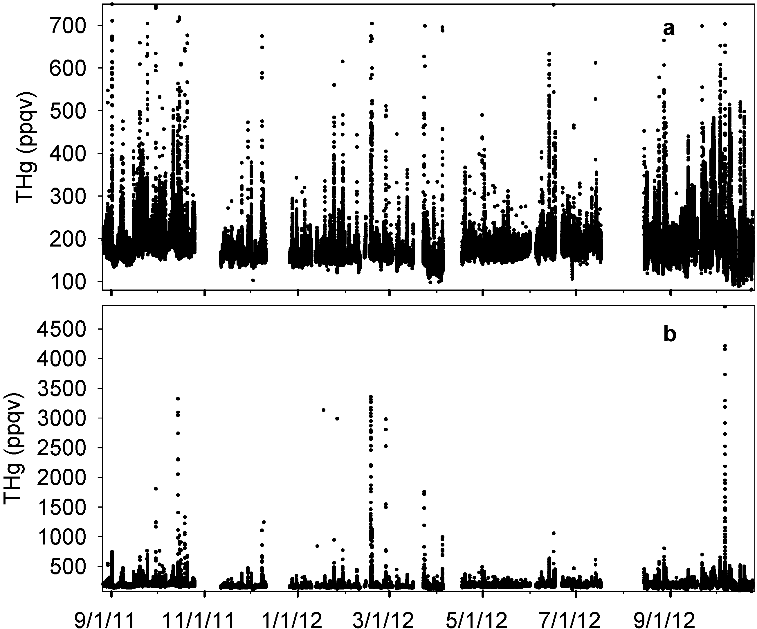
The complete time series of THg is presented in Figure 2. The median level of THg in Houston was 172 ppqv (181 ± 63 ppqv for mean ± S.D.) during our observation period (see Figure S2 and Table S1 for more statistical details), which was in agreement with the current background level in the Northern Hemisphere [20], but slightly lower than other urban sites with mercury levels higher than 2 ng∙m⁻³ (224 ppqv) [22,25,28,39,40]. The majority of THg observations fell within the range of 148 ppqv (10th percentile) to 215 ppqv (90th percentile). The maximum THg mixing ratio, however, was as high as 4876 ppqv, exceeding 25 times the current global background level. The minimum level was 80 ppqv, which occurred with southerly wind that brought cleaner air from the Gulf of Mexico into urban Houston. A prominent feature of THg in the Houston area was the frequent occurrence of large THg spikes (Figure 2b). From 14-month measurements, we documented 81 well-developed spikes with THg levels higher than 300 ppqv, 34 of which were higher than 500 ppqv. Extremely large peaks with THg levels higher than 1000 ppqv were observed 12 times, and six of them were higher than 3000 ppqv. The time scale of elevated mercury in these spikes ranged from 30 minutes to a few hours. As a consequence of the THg spikes, the standard deviations of our data reached 63 ppqv, which was comparable with other urban sites measurements, such as Salt Lake City (95 ppqv [22]) and Reno (45–90 ppqv [39]).

Figure 2. Complete time series of THg from MT measurements. (a) and (b) show the same data with different ranges in y axis.

Figure 2. Complete time series of THg from MT measurements. (a) and (b) show the same data with different ranges in y axis.

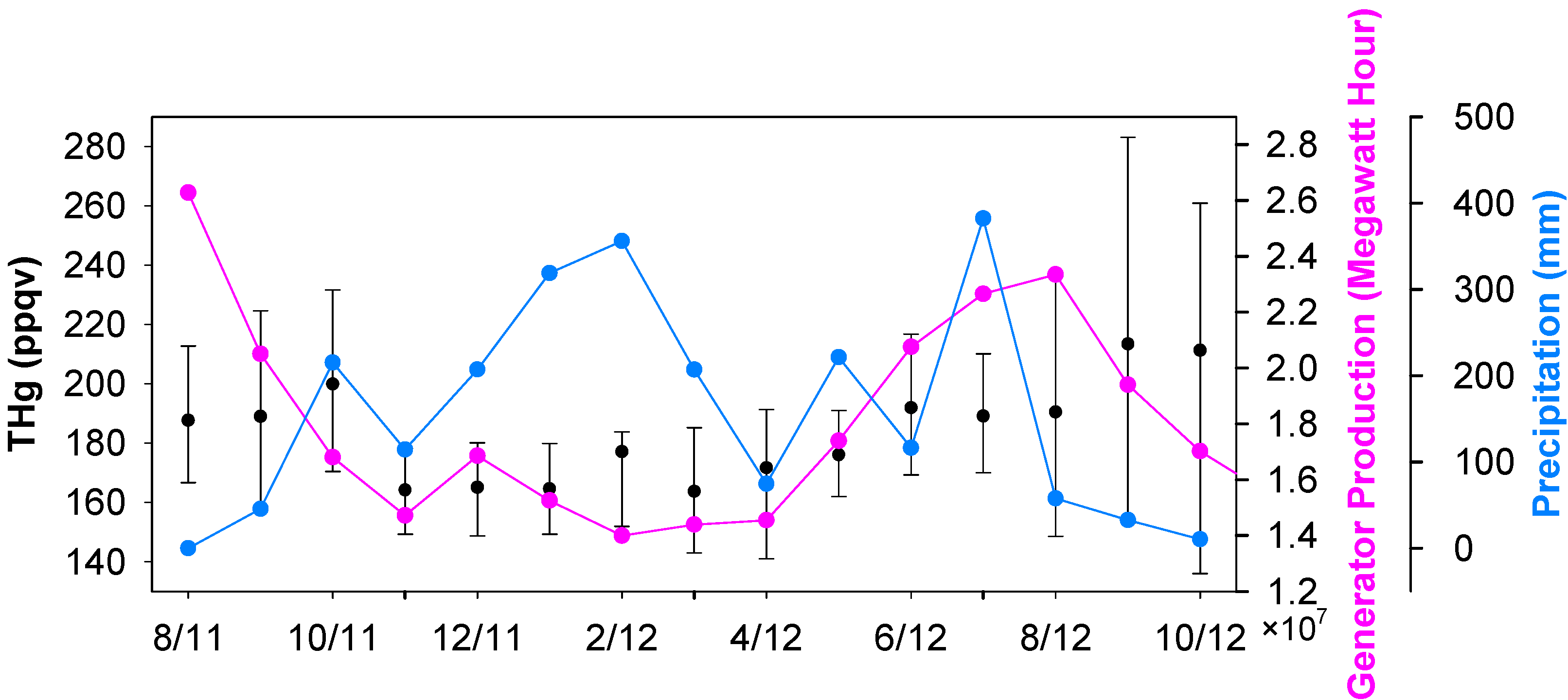
Seasonal median levels of THg were 178 ppqv (179 ± 54 ppqv for mean ± S.D.), 161 ppqv (161 ± 80 ppqv), 172 ppqv (172 ± 26 ppqv), and 185 ppqv (186 ± 32 ppqv) for fall 2011, winter 2011, spring 2012 and summer 2012, respectively. The monthly median THg values are displayed in Figure 3. Unlike many other ambient mercury measurements, which show higher mercury in winter time [21,22], high THg in Houston area occurred in the warm seasons (June to October). It is obvious that the frequent occurrences of large THg spikes during the warm seasons, especially in August, September and October, contributed to the elevated THg levels. The great enrichments in episodic THg spikes suggested that the large pollutant plumes originated from the nearby industrial/urban emission sources. Mercury emissions from anthropogenic sources are closely linked to energy production, especially from coal-fired power plants, the largest anthropogenic mercury source in U.S. [13]. Enhanced energy production is expected in the Houston area in summer and fall. The high ambient air temperature requires energy to operate air-conditioning units. As a consequence, the ambient THg levels may increase. To illustrate this point, the state-level energy data achieved from Energy Information Administration (EIA) is presented in Figure 3. The monthly total energy produced in warm months was 50%–100% higher than in the cold months (The correlation coefficient between monthly median THg and monthly median energy production is 0.735, which is statistically significant (p ≤ 0.005)). Besides the fluctuations in mercury sources, we noticed some changes in potential sinks. Mercury deposition in rain water has been commonly reported [41,42,43], indicating rainfall as an important removal mechanism for atmospheric mercury. The precipitation in Houston was observed to be consistently higher in the period from December 2011 to March 2012 (Figure 3), which coincided with low wintertime THg.

Figure 3. Monthly medians of THg, energy production and precipitation.

Figure 3. Monthly medians of THg, energy production and precipitation.

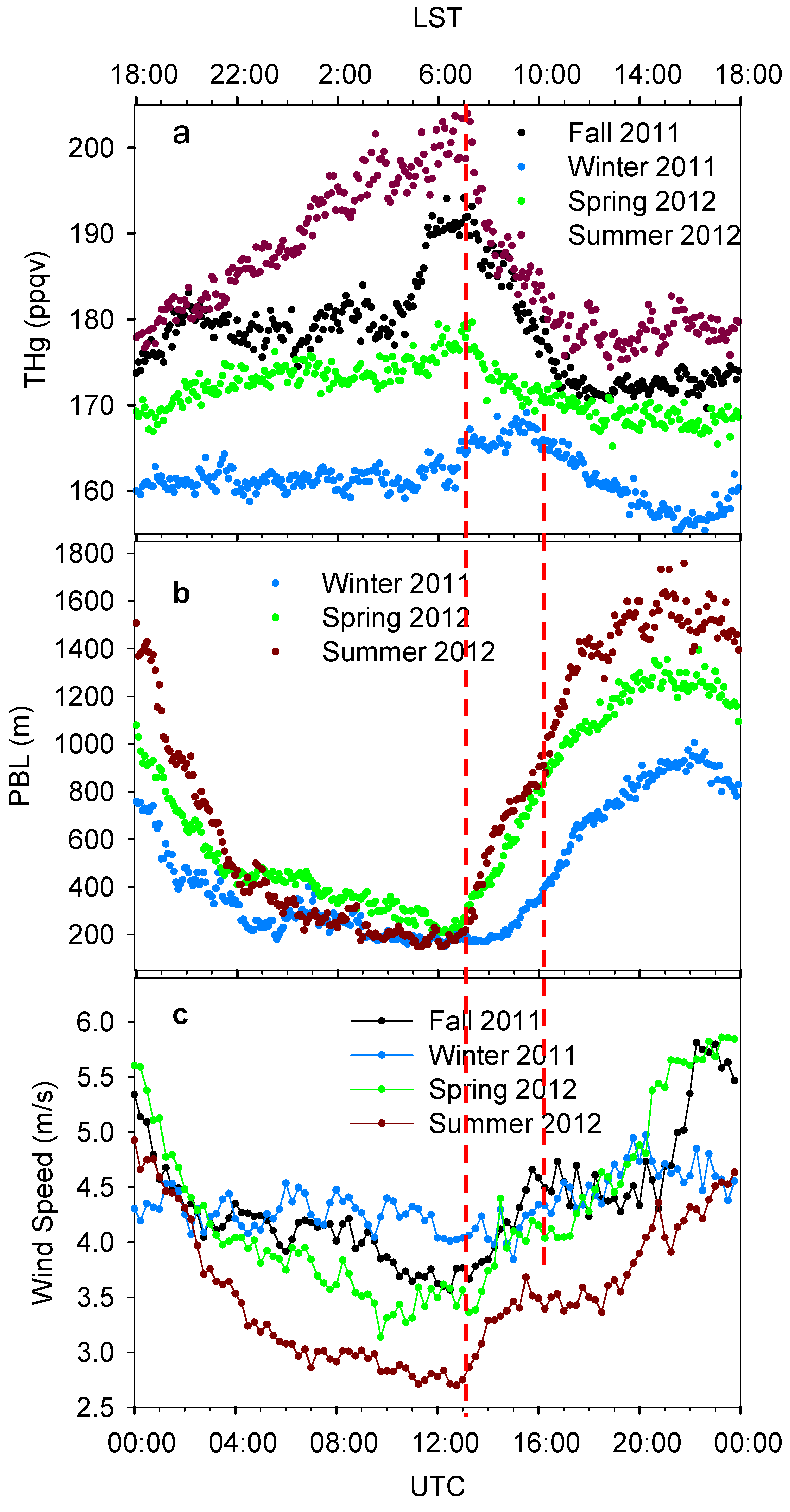
Precipitous day-to-day peaks and valleys variations were also observed as another outstanding feature of THg signal. Hourly median THg mixing ratios are displayed in Figure 4a. Despite the differences in variation amplitudes, diurnal variation patterns in fall, winter and spring were generally similar. Their diurnal patterns show a period with increasing THg levels starting around 16:00–18:00 local standard time (LST) and lasting for 2–4 hours, followed by a period with relatively constant THg levels. A sharp enhancement of THg levels started at around 04:00 LST, and then the THg reached a daily maximum at 07:00–09:00 LST. The summer diurnal pattern, however, appeared to be very different from other seasons. The THg level in summer gradually increased throughout the whole night and reached its maximum at about 07:00 LST, indicating an accumulation process of THg. Summertime had the highest THg mixing ratios during a day, and the largest diurnal variation amplitude (about 30 ppqv) among the four seasons. To conclude, the THg levels were higher at night than during the daytime. The maximum levels appeared right before sunrise, followed by rapid decreases after sunrise, and daily minimum shortly after noon. Similar diurnal patterns were observed in other urban cities, such as Guiyang, China [27], Detroit, U.S. [28], and Toronto, Canada [29].

It is interesting to note that the THg mixing ratio reached its diurnal maximum at about 07:00 LST in fall, spring and summer, while it was two hours later in winter. This phenomenon was related to the diurnal development of the PBL (Figure 4b). The PBL heights started increasing at about 06:00–07:00 LST for spring and summer and two hours later for winter. The rapid enhancements of PBL height in early morning can facilitate air mixing in three-dimensions and dilute the ambient THg within the boundary layer, and thus caused striking decreases of THg at the same time. The rate of decrease in summer was the largest (7.0 ppqv∙h⁻¹), compared to those in winter (1.9 ppqv∙h⁻¹), spring (2.6 ppqv∙h⁻¹), and fall (4.6 ppqv∙h⁻¹). The high PBL height in daytime then contributed to the low THg mixing ratios, especially in the afternoon. This phenomenon suggested that the residual layer was not a significant source for THg in Houston; instead, the industrial/urban emissions from the surface were more prominent.

Figure 4. Seasonally diurnal variations of THg (a), PBL height (b) and horizontal wind speed (c). Data shows the median values with 5 min. time interval. The top x axis shows time in LST and the bottom x axis shows time in UTC. LST = UTC − 6:00.

Figure 4. Seasonally diurnal variations of THg (a), PBL height (b) and horizontal wind speed (c). Data shows the median values with 5 min. time interval. The top x axis shows time in LST and the bottom x axis shows time in UTC. LST = UTC − 6:00.

However, some features of the diurnal THg variations cannot only be explained by the PBL height propagations, for example, the summertime THg mixing ratios were the highest during all times of the day even though the daytime PBL heights were the highest. It was observed that the diurnal variations of horizontal wind speeds were anti-correlated with THg levels most of the time (Figure 4c, median wind speeds were calculated using scalar values). High horizontal wind speeds can enhance horizontal mixing of polluted air with cleaner ambient air, and effectively advect the pollutants away from the urban area. The summertime wind speed was the lowest of all seasons, and the especially low wind speeds at night supported the accumulation of THg and caused high summertime THg mixing ratios. In spring, low wind speeds were observed at 04:00–07:00 LST, which probably contributed to the high THg mixing ratios in this period.

The energy production/consumption, precipitation, PBL height, and horizontal wind speed played important roles in the seasonal and diurnal variations of THg; however, we cannot quantify the contribution of each factor from our observations. Regional modeling with a good emission inventory and dynamic processing is necessary for further investigation.

It is unclear whether photochemical reactions play an important role in determining THg mixing ratios in the Houston area. Previous research suggests that the main sink of GEM in the atmosphere is oxidation to GOM [44]. The GOM then can attach to particles and be transformed to PBM. Both GOM and PBM are easily removed from the air via wet and dry deposition [21,45], which will eventually reduce the mixing ratio of THg. From our observations, the diurnal THg mixing ratios remained constant from 12:00 LST to 16:00 LST in fall, spring and summer. During these times, photochemical reactions should be actively changing due to the fluctuations of solar radiation and variations in the abundance of oxidants. The effect of photochemical reactions may be obscured due to complex local emissions and meteorological conditions.

Natural sources can also influence the seasonal and diurnal variations of ambient THg levels; however, we are unable to quantify the contributions of natural emissions in metropolitan Houston due to a lack of direct measurements. However, a large portion of vegetation in the Houston area is evergreen; with no snow in winter, we expect small contributions from natural emissions to the THg seasonal variations.

2.2. Wind Induced Influences

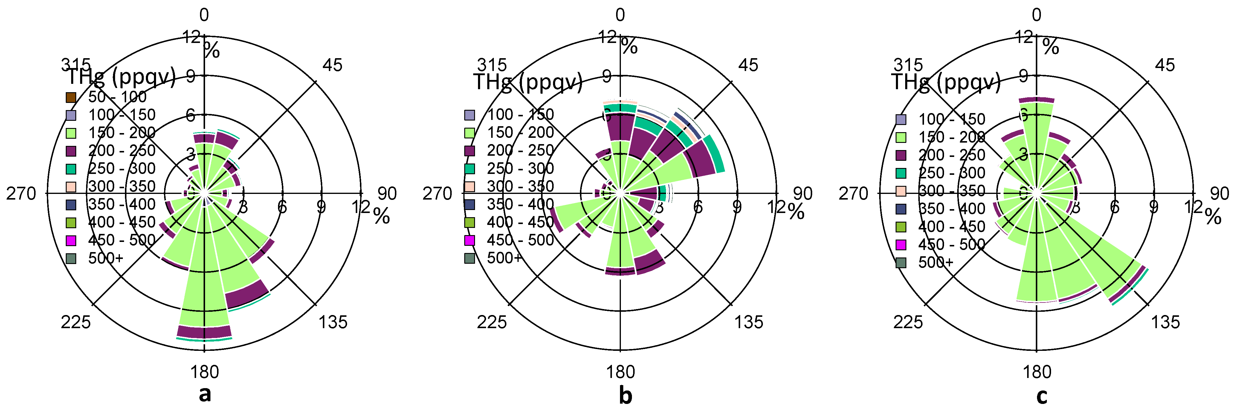
In addition to the wind speed, the wind direction also exerts considerable impacts on THg variations, suggesting the importance of local/regional transport. In Figure 5, the percentage values on the R axis shows the frequency (%) of THg coming from a certain range (22.5°) of wind directions. The predominant wind directions in our observed period were south and southeast directions (120°–190°) (Figure 5a), which were from the Gulf of Mexico. The overall frequency from these directions accounts for about 40%, after summing up the percentage values from 120°–190° directions in Figure 5a. Cleaner air masses with especially low THg levels (<150 ppqv) were observed from these directions. However, the refinery facilities emissions in Texas City may also advected to Houston area as we obtained about 6% of air masses with THg levels higher than 200 ppqv from the same directions.

Figure 5. Complete THg versus wind direction (a), THg versus wind direction in HMP (b), THg versus wind direction in LMP (c). The color scale shows the ranges of THg mixing ratios. The percentage values on the R axis shows the frequency of THg coming from a certain range (22.5°) of wind directions.

Figure 5. Complete THg versus wind direction (a), THg versus wind direction in HMP (b), THg versus wind direction in LMP (c). The color scale shows the ranges of THg mixing ratios. The percentage values on the R axis shows the frequency of THg coming from a certain range (22.5°) of wind directions.

Wind direction in Houston varied diurnally. From Figure 4a, we noticed elevated THg mixing ratios at about 05:00–11:00 LST, and lower mercury mixing ratios at about 12:00–17:00 LST. To evaluate the impacts of shifting wind direction, we defined a daily high mercury period (HMP) of 05:00–11:00 LST and a daily low mercury period (LMP) of 12:00–17:00 LST. Figure 5b,c depict the wind rose for HMP and LMP in 2011 fall, respectively. In the HMP, air masses with high THg levels (200 ppqv) mainly came from north, northeast, and east sectors, where urban and industrial influences were remarkable, especially in the Houston Ship Channel area. In the LMP, air masses mainly came from the south and southeast sectors, where cleaner marine air seemed to dominate. The median THg level in HMP was statistically higher than that in LMP (14 ppqv higher, p ≤ 0.001). Analysis of other seasons (not shown) also suggested similar influences from shifting source regions. It was also observed that consistent northerly winds with high wind speeds (>4 m/s, occurred in December) yielded THg levels ≥ 150 ppqv, and CO levels ≥ 125 ppbv. In comparison, consistent southerly winds with high wind speeds (occurred in April) produced THg levels as low as 120 ppqv and CO levels as low as 85 ppbv. The large discrepancies between southerly air and northerly air highlight the significance of local urban/industrial influences on elevated THg mixing ratios in the Houston area.

The sea breeze exerted significant and complex impacts on THg levels in the Houston area. The sea breeze is driven by diurnally uneven heating in coastal areas, which produces warmer temperatures over land than over water during the day, and cooler land temperatures at night [46]. As a result, a sea breeze is produced when the air flows from the sea to the land at low altitude (<500 m). The low level wind vector then rotates through a clockwise (Northern Hemisphere) cycle under the influence of the Coriolis force [46,47]. As the sea breeze passes through the shoreline, it can bring cleaner marine air to inland areas that can dilute urban/industrial emissions. The sea breeze can also bring back ashore the aged polluted air that was once transported offshore by other wind systems. A detailed analysis on the wind system in Houston area reported that the afternoon sea breeze was responsible for large O₃ enrichment events, by bringing back aged, polluted air masses to the urban area [46].

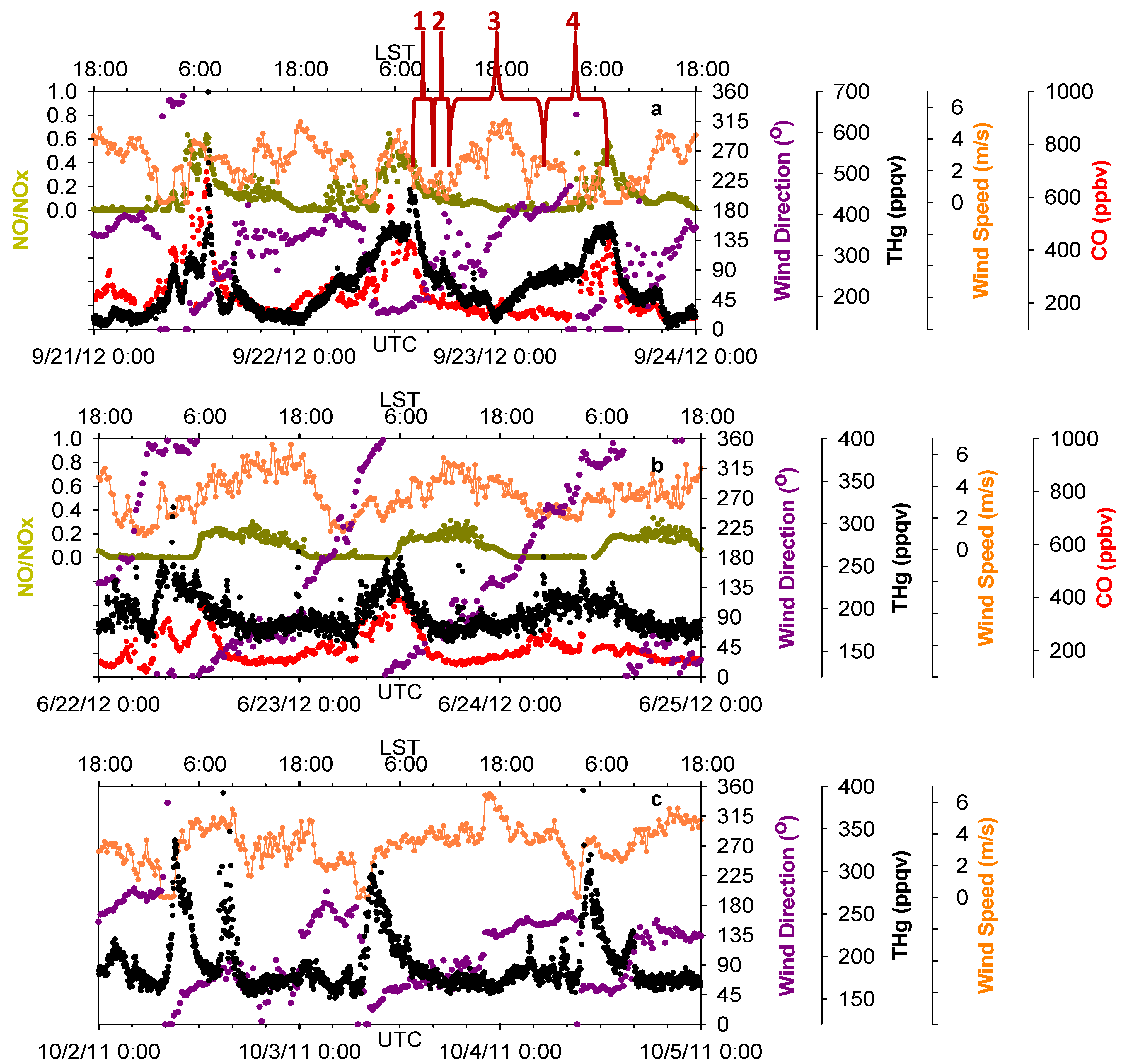
Figure 6. Time series of THg, CO, NO/NO_x, wind speed and wind direction. (a,b,c) show the influences of three common wind patterns on THg levels.

Figure 6. Time series of THg, CO, NO/NO_x, wind speed and wind direction. (a,b,c) show the influences of three common wind patterns on THg levels.

Our observations found similar effects from the bay breezes (from Trinity Bay and Galveston Bay, southeast of MT) and the sea breeze (from the Gulf of Mexico, south of MT). Figure 6a presents an example of sea breeze impacts on THg diurnal variations. Four stages of THg variations with corresponding wind shifts are marked for illustration. In stage one, THg mixing ratios decreased significantly, partially because of the increase in PBL height, and also the northerly winds that were controlling this area and pushing the urban pollutants offshore. In the second stage, the bay breeze and sea breeze built up and intruded inland as southerly winds. The bay breeze and sea breeze then moved into urban Houston, where they met the northerly flow and formed a sea breeze front. With the influence of a sea breeze front, the horizontal wind speeds decreased to less than 2 m/s, causing a stagnant period, which would not favor vigorous air diffusion or transport. In addition, the polluted flow transported offshore then returned back to Houston with the southerly winds. We observed slightly elevated THg and CO in this period. It is known that NO/NO_x can serve as an indicator for the relative age of air masses, because of the short life time of NO. The NO/NO_x values in this stage were less than 0.3, indicating the influences of aged air masses in which NO was oxidized. In this stage, a convergent zone formed where sea breeze front was concentrated. As a result, the updraft can bring polluted air to higher altitudes and enable long-distance transport of THg. In the third stage, the sea breeze moved farther inland and cleaner marine air behind the sea breeze front controlled air quality in the Houston area. The THg levels were observed to be the lowest of the day. In the final stage, the sea breeze faded out at night and northerly wind again controlled this area. Significant enhancement of THg occurred within the nocturnal boundary layer, along with high CO and NO/NO_x (~0.6), indicating the influences of fresh urban/industrial emissions. These four stages occurred frequently day-to-day during the warm season.

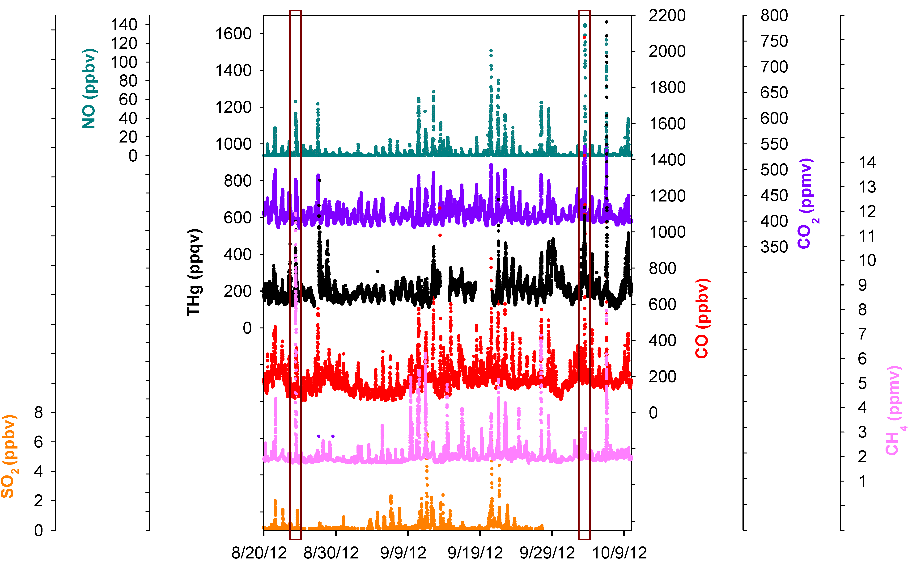
Figure 7. Time series of THg, CO, CO₂, NO, SO₂, and CH₄. The two boxes are comparisons of two episodes with different CH₄ mixing ratios.

Figure 7. Time series of THg, CO, CO₂, NO, SO₂, and CH₄. The two boxes are comparisons of two episodes with different CH₄ mixing ratios.

Another diurnal pattern of THg that also involved the sea breeze is depicted in Figure 6b. Clockwise rotation of wind directions diurnally were accompanied with obvious THg diurnal changes in which daily low THg mixing ratios occurred when winds were southeast and southerly flow dominated. The diurnally 360° changes in wind direction occurred in March through October, but not in November through February. This pattern was documented on about 30 days in our 14-month data span. Another interesting feature we observed in THg diurnal patterns was that THg levels tended to peak right after abrupt changes in wind direction (45 degree change, normally from south winds to north winds), with few exceptions. This condition occurred on 90 days over 14 months, while the wind shifts occurred mostly around 02:00–04:00 LST (Figure 6c). Please note that while sea breeze constantly corresponds with relatively low levels of THg in the afternoon and early evening in Figure 6b,c, the aged plumes were not always observed as in Figure 6a, which may due to the differences in the strength (relative to northerly) and the daily propagation of the sea breeze.

2.3. Relationship of THg with Key Trace Gases

An advantage of this study was that multiple trace gas species were sampled at the same location (MT) along with THg with high time resolutions. Investigating the relationships between THg and other key trace gases can provide important information concerning mercury sources. Figure 7 displaced the time series of SO₂, NO, CO, CO₂, CH₄, and THg. 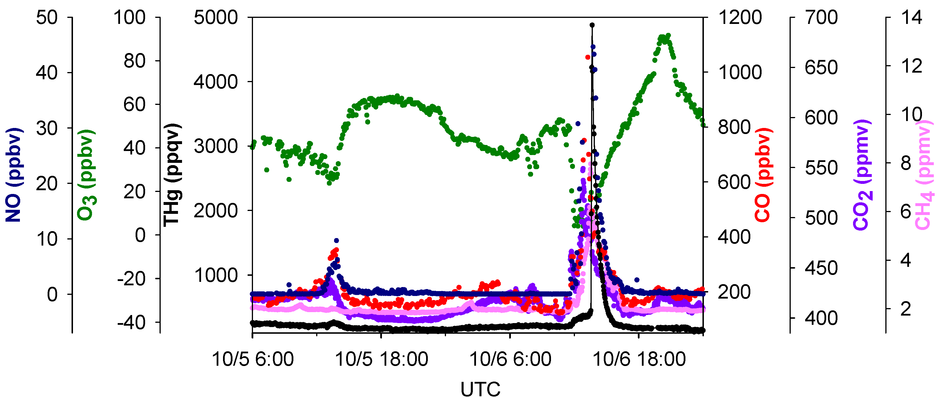A significant feature we noticed was the common co-occurrence of THg peaks with SO₂, NO, CO, CO₂, CH₄ peaks in pollution plumes. A zoom-in picture depicting the maximum THg spike observed during this study is presented in Figure 8. This episode corresponded with air masses coming from the northeast of our sampling site, which is the direction of Houston Ship Channel. This highly concentrated pollution plume with THg mixing ratios as large as 4876 ppqv was related to combustion tracers, such as CO, CO₂, and NO. In addition, this THg peak occurred coincidentally with a peak in CH₄, which is presumably released from oil and natural gas operations, landfills, and waste treatment facilities. In this episode significant enhancements of NO, THg, CO, CO₂, and CH₄ started at 04:30 LST and peaked at 06:45–07:45 LST. The maximum levels of each species in this plume were 4876 ppqv for THg, 1053 ppbv for CO, 45 ppbv for NO, 549 ppmv for CO₂ and 8.0 ppmv for CH₄. The close correspondence between THg and other species in the THg episodes is clearly evident, and thus it is possible that THg came from similar sources as some of the other trace gases. However, the peaks signatures varied greatly in different pollution plumes. Extreme THg peaks sometimes were in conjunction with exceptional large peaks of CH₄ (e.g., Figure 7 left box, 11.8 ppmv), but sometimes with slightly elevated CH₄ (e.g., Figure 7 right box, 3.1 ppmv). Correlations of THg with other trace gases were diffuse overall; correlation coefficients (R values) between THg and those species were low (R < 0.43, see Table S2) albeit their correlations were statistically significant (95%), suggesting the possible contributions from diverse source types in the Houston area.

Figure 8. Time series of THg, CO, CO₂, NO, O₃ and CH₄ in the largest THg plume.

Figure 8. Time series of THg, CO, CO₂, NO, O₃ and CH₄ in the largest THg plume.

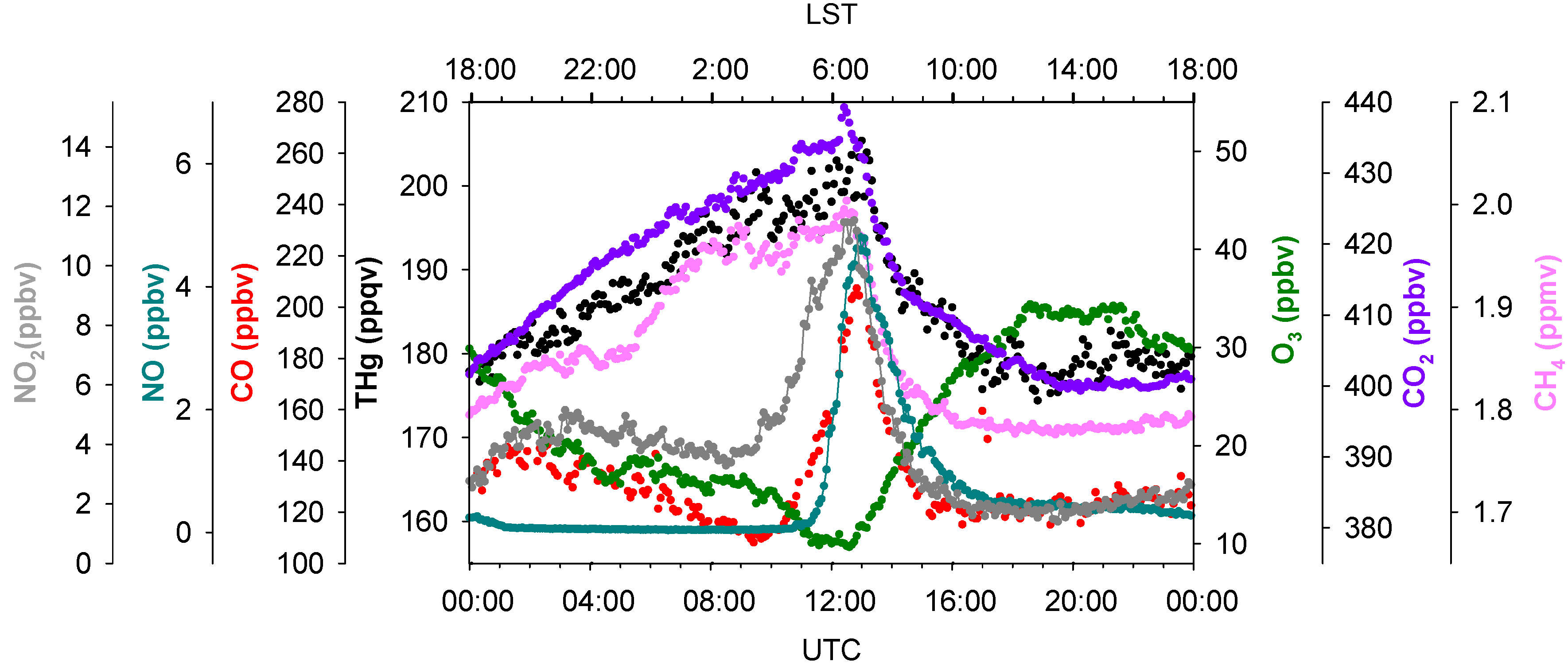
Detailed analyses of diurnal variations of THg and other species can also provide valuable information on mercury sources and sinks. Figure 9 exhibits the summertime diurnal variations of THg, NO, NO₂, CO, O₃, CO₂, and CH₄. Interestingly, THg, CO₂ and CH₄ had similar diurnal patterns; however, it is still difficult to determine whether these patterns were resulting from meteorological forcing, such as PBL height and winds, and/or their similar emission sources. The diurnal patterns of NO, NO₂, and CO, were ubiquitously distinguished from those of THg, CO₂, and CH₄. Vehicle emissions are believed to be the dominant sources of NO, NO₂, and CO in urban areas [48,49]. We noticed that the mixing ratios of CO and NO₂ started increasing simultaneously at 03:30 LST (04:30 Local Daylight Saving Time) and reached their maximums at 06:00–07:00 LST. The mixing ratios of NO started increasing after sunrise, about two hours later compared to NO₂ and CO. Ozone titration was also observed at the same time when elevated CO and NO₂ occurred (note that O₃ photochemistry in this site is limited by VOCs, instead of NO_x [50]). We believe these were traffic signals; NO was emitted by vehicles subsequently titrating O₃ and being converted to NO₂, but without sunlight NO₂ builds up. The diurnal pattern of THg tracked those of CO₂ and CH₄, instead of CO and NO₂, suggested that vehicle emissions may not exert outstanding impacts on THg levels in summer. The importance of vehicle emissions as a THg source is yet to be further investigated.

Figure 9. Diurnal variations of THg, CO, CO₂, NO, NO₂, O₃ and CH₄ in summer 2012. Data shows the median values within a 5 min. time interval.

Figure 9. Diurnal variations of THg, CO, CO₂, NO, NO₂, O₃ and CH₄ in summer 2012. Data shows the median values within a 5 min. time interval.

2.4. Mercury Episodes

As we reported previously, 81 spikes were documented with THg mixing ratios greater than 300 ppqv. We calculated the enhancement ratios (ER) in these plumes to retrieve information about point sources. Enhancement ratios are obtained by dividing the excess species (THg in this study) concentrations measured in a pollution plume by the excess concentration of a reference gas, for example, CO₂, CO and CH₄ in this study. Enhancement ratios are commonly expressed in molar ratios, and the ambient background levels of each gas must be subtracted to get the “excess” values. For example, the ER for THg relative to CO is:

(1)

Enhancement ratio is a different parameter compared to emission ratio because the measurement is conducted from a downwind location instead of at the source. Since THg, CO, CO₂ and CH₄ are not highly reactive species, it is possible that ERs remain close to emission ratios of a specific source in short-distant transport. Further we may assume that pollution plumes coming from the same direction were from the same emission source if they have similar ERs. For ER calculation, we characterized the air masses with the lower 25th percentiles of CO mixing ratios as background air [23], and the corresponding medians values for this part of data were used as the background levels so as to minimize the possible influence of local sinks. Those values were 172 ppqv for THg, 112.6 ppbv for CO, 1.79 ppmv for CH₄, and 403.3 ppmv for CO₂. 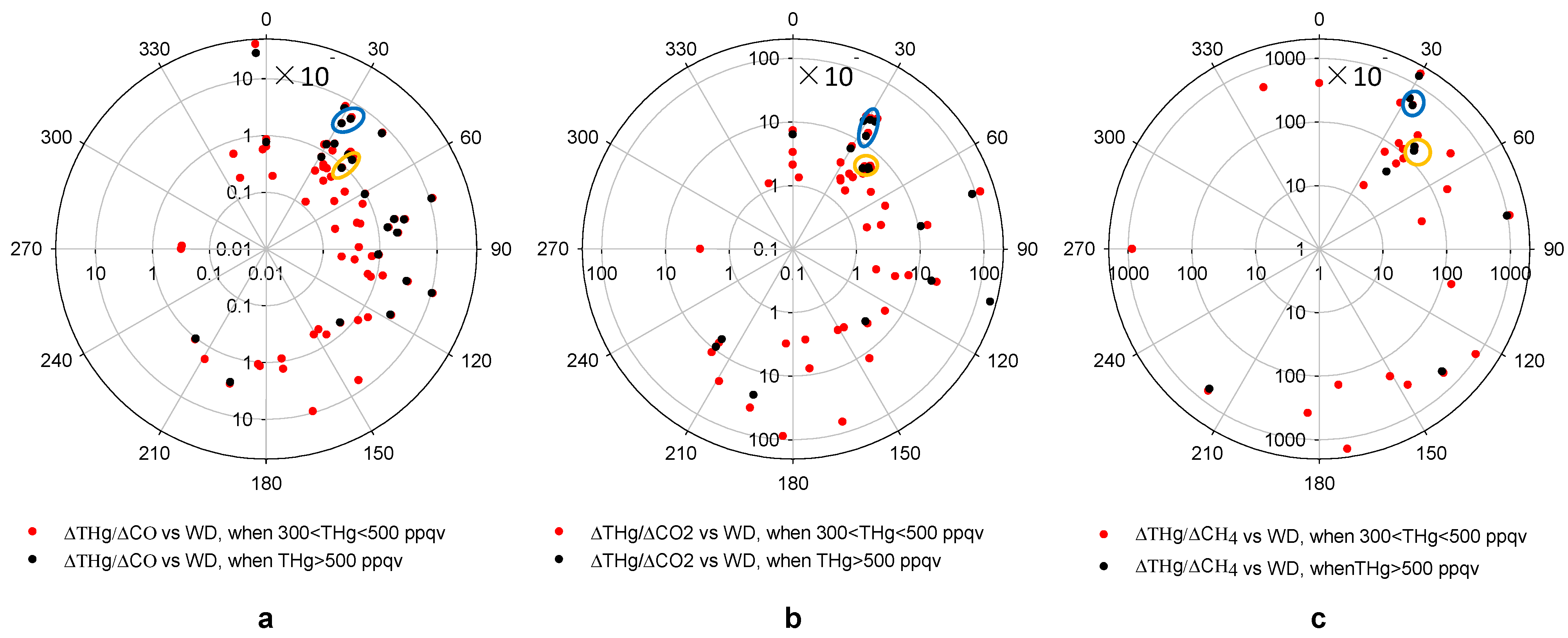Figure 10 presents the ER values for ∆THg/∆CO, ∆THg/∆CO₂ and ∆THg/∆CH₄, versus wind directions. The CO₂ measurements are only available from March 2012 and CH₄ measurements from June 2012. Thus, fewer episodes were available for ∆THg/∆CO₂ and ∆THg/∆CH₄ compared to ∆THg/∆CO.

The patterns of ∆THg/∆CO and ∆THg/∆CO₂ versus wind direction shared some similarities (Figure 10). Pollution plumes with THg mixing ratios higher than 500 ppqv tended to produce higher ERs, compared to those with THg mixing ratios between 300 ppqv and 500 ppqv. A large percentage of THg episodes with high CO or CO₂ mixing ratios originated from the 30°–120° direction, the Houston Ship Channel area. Note that, from Figure 5a, air masses from this direction only accounted for about 17% of the total air mass measured at MT. This means that most THg episodes originated from directions that were the least favored wind directions.

Figure 10. Enhancement ratios versus wind direction in high THg episodes.(a,b,c) show ∆THg/∆CO, ∆THg/∆CO₂ and ∆THg/∆CH₄ versus wind direction, respectively. The yellow circles point out two ERs potentially from the same source at ~40° direction and the blue circles represent another two episodes from a source at ~30° direction.

Figure 10. Enhancement ratios versus wind direction in high THg episodes.(a,b,c) show ∆THg/∆CO, ∆THg/∆CO₂ and ∆THg/∆CH₄ versus wind direction, respectively. The yellow circles point out two ERs potentially from the same source at ~40° direction and the blue circles represent another two episodes from a source at ~30° direction.

For now, we are unable to correlate these pollution plumes with specific sources due to the absence of detailed and accurate source signatures. The EPA NEI [13] provides annual total emissions for THg and CO, and the Greenhouse Gases (GHGs) Emissions Data [51] also provides annual total emissions of CO₂ and CH₄ for significant emission sources. We attempted to compare our ER values with emission ratios calculated from the EPA inventory. In the northeast direction from MT, the direction with a large number of THg episodes, we found only 2 point sources within a short distance (<80 km) from MT that were documented in the 2008 EPA NEI as mercury sources. From the ER versus wind direction plot, we noticed 2 episodes with similar ∆THg/∆CO, ∆THg/∆CO₂ and ∆THg/∆CH₄ values from the 40° direction (Figure 10, yellow circles). Considering the large elevations of THg, CO, CO₂ and CH₄ in these episodes, we suspect that they could be attributed to local sources. A waste treatment facility located about 5 km away from MT in that direction was reported by the 2008 NEI and 2010 GHGs Emissions Data as a source for THg, CO, CO₂ and CH₄. The other point source that was likely associated with another 2 episodes with similar ∆THg/∆CO, ∆THg/∆CO₂ and ∆THg/∆CH₄ values were from the 30° direction (Figure 10, blue circles). We found an iron and steel casting facility from EPA NEI 9 km away from MT. Table 1 shows the comparisons between ER values calculated from observations and emission ratios calculated from the EPA inventory (please note that this iron and steel casting facility is not listed in the 2010 GHGs Emissions Data, which may be due to the fact that the 2010 GHGs Emissions Data does not include sources that have annual emissions of less than 25,000 metric tons of CO₂e. For the emission ratios calculations, we assume the CO₂ and CH₄ emissions from this facility were 25,000 metric tons of CO₂e). The differences between these two ratios were significant, up to a few orders of magnitude. It is highly possible that the EPA emission inventory may have inaccurate estimations of the total emissions. It is also possible that some emission sources may not be documented in the EPA inventory.

Table 1. Comparisons between ER values derived from MT observations and emission factors calculated from EPA Inventory.

Facility	∆THg/∆CO		∆THg/∆CO2		∆THg/∆CH4
	EPA	Observation	EPA	Observation	EPA	Observation
30°, Iron and steel casting (blue circles)	1.77 × 10−5	8.9 × 10−7~1.49 × 10−6	5.04 × 10−7	5.3 × 10−9	9.78 × 10−3	1.40 × 10−7
40°, Waste treatment (yellow circles)	5.70 × 10−8	3.7 × 10−6 ~5.4 × 10−6	1.77 × 10−10	1.3 × 10−8~2.3 × 10−8	1.35 × 10−9	5.0 × 10−7~5.8 × 10−7

Table 1. Comparisons between ER values derived from MT observations and emission factors calculated from EPA Inventory.

Facility	∆THg/∆CO		∆THg/∆CO2		∆THg/∆CH4
	EPA	Observation	EPA	Observation	EPA	Observation
30°, Iron and steel casting (blue circles)	1.77 × 10−5	8.9 × 10−7~1.49 × 10−6	5.04 × 10−7	5.3 × 10−9	9.78 × 10−3	1.40 × 10−7
40°, Waste treatment (yellow circles)	5.70 × 10−8	3.7 × 10−6 ~5.4 × 10−6	1.77 × 10−10	1.3 × 10−8~2.3 × 10−8	1.35 × 10−9	5.0 × 10−7~5.8 × 10−7

3. Experimental Section

Continuous THg measurements were conducted atop Moody Tower (29.71°N, 95.34°W), an elevated site (75 m above ground level) located on the main campus of the University of Houston (Figure 1). This urban site is located about 2–4 km away from major freeways and industrial facilities, and 4–5 km away from downtown Houston. The campus is surrounded by vegetation covered land surfaces. It is 35 km west of the Galveston Bay and 70 km northwest of Galveston, TX and the Gulf of Mexico. The data reported in this study was acquired from 26 August 2011 to 25 October 2012.

Total gaseous mercury was measured with a Tekran 2537A automated instrument. The Tekran instrument uses cold vapor atomic florescence (CVAF) detection in sequential dual channels with 2.5 min. time interval resolution, yielding a detection limit of 5–10 ppqv. A Teflon filter (1 µm pore size) was used to remove aerosols at the entrance of the inlet, and was changed weekly. The sample line was 6 m long and composed of Silco-Steel Sulfinert coated (Restek) stainless steel. We conducted extensive testing of the passing efficiency of GOM through Silco Steel Sulfinert tubing using permeation sources of HgBr₂ and HgCl₂. This tubing passed these two mercury species with 100% efficiency. Heating of the tubing was not required to attain this high passing efficiency. We also tested teflon filters and found 100% passing efficiency at the flow rates used for sampling. Instrument calibration was checked weekly using the internal mercury permeation source. The internal standard was verified every six months using a Tekran 2505 unit. Judging from the inter-comparison with 2 other co-located Tekran instruments, the overall precision of this instrument was ± 10% [34]. The accuracy of the mercury measurement was estimated to be ± 5%. In this work, mercury is reported using mixing ratios in ppqv so that it is directly comparable with other trace gases. Under Standard Temperature and Pressure conditions, 1 ng∙m⁻³ equals to 112 ppqv. Except for the time series analysis, the THg data was averaged to 5 min. for various comparisons.

Carbon monoxide was measured using a Thermal Environmental (TE) CO Analyzer (48C-TLE). Ozone was measured with a TE O₃ U.V. photometric analyzer (49C). Sulfur dioxide was measured using a TE 43C instrument. The CO, O₃, and SO₂ analyzers shared the same inlet, whose sample lines were around 10–12 m long. Nitric oxide, nitrogen dioxide and NO_x were measured using the TE NO-NO₂-NO_x chemiluminescence analyzer (42C) with a blue light converter to photolyze NO₂ to NO. The inlet of NO-NO2-NOx analyzer was 5 m away from the inlet of inlets of CO, O₃, and SO₂ analyzers, and the sample line was 7.5 m long. These inlets used PFA Teflon tubing, and both of them were about 6 m away from the THg inlet. To maintain accurate measurements, these four instruments were adjusted to zero and the span checked on a daily basis. Multi-point calibration was conducted every two weeks. The original time resolution of CO, O₃, SO₂, NO, NO₂, and NO_x was 10 s, and these data were average to 5 min. in this study. Carbon dioxide was measured using a LI-COR LI-7000 analyzer and CH₄ was measured with a PICARRO G2132-i instrument. Both instruments calibration was checked monthly using standards obtained from Scott-Marrin with ±1% NIST traceable quality. The sample lines of LI-COR and PICARRO instruments were about 6 m long, and their inlets were co-located with THg inlet. The original time resolutions of CO₂ and CH₄ were 1 min. and 1.5 s, respectively. Except for the time series analysis, both dataset were average to 5 min. for comparison to other species.

Basic meteorological parameters, including ambient temperature, wind speed, wind direction, precipitation, relative humidity, and pressure were monitored with a collection of Campbell Scientific sensors with 10 s resolution and averaged to 5 min. for this study.

Planetary boundary layer (PBL) height was measured at another site (29.72°N, 95.34°W), also located on the main campus of University of Houston. This was a ground level site, about 700 m away from Moody Tower site. A Vaisala CL31 Ceilometer was used to measure PBL height with 5 m height resolution, and PBL height was reported every 5 minute. The PBL height measurements from this instrument agreed very well with our radiosonde and ozonesonde measurements. More details concerning the performance and algorithm settings of this instrument are discussed in Haman et al. [52].

4. Conclusions

This study provides the first assessment of mercury pollution in the highly populated and industrial city of Houston, Texas. Our continuous measurements show that the median THg level was consistent with the current global background level; however, a predominant feature of THg in the Houston area was the frequent occurrence of large peaks (≥300 ppqv). The primary focus of this study has been placed on characterizing the seasonal and diurnal variation patterns of THg in Houston. We found that the highest seasonal median THg mixing ratios occurred in summer and the lowest ones occurred in winter. The seasonal patterns of THg were closely linked to the frequency of THg episodes, and also the energy production/consumption and precipitation (rainfall) in the area. Diurnally, the THg levels were higher at night than at daytime. The maximum THg levels appeared right before sunrise, followed by rapid decreases after sunrise. The diurnal variations were clearly under the influence of PBL height and horizontal winds, including the complex sea breeze system in the Houston area. Our results combined with those of Banta et al. [46] suggest a very active influence of the sea breeze in the Houston area, which can either increase or decrease the urban THg levels over a day depending on the position of the sea breeze front.

Special emphasis has been placed on the THg episodes. Highly concentrated pollution plumes originated from urban Houston agglomeration revealed that THg levels were related to the combustion tracers such as CO, CO₂, and NO. The occurrences of THg peaks also coincided with peaks in CH₄, which was presumably released from oil and natural gas operations, landfill, and waste treatments. The frequent co-occurrences of THg episodes with peaks in CO, CO₂, CH₄, NO_x, and/or SO₂ suggested possible contributions from similar sources. We noticed that the majority of the THg episodes were from the Houston Ship Channel Area. When our observed ERs values were compared with the emission ratios calculated from the annual total emissions documented by EPA inventory, we found that the EPA 2008 NEI and 2010 GHGs Emissions Data may not reflect the actual emissions from industrial facilities.

Future work is warranted to quantify the contributions of each factor on THg variations. This study established a strong connection between PBL height and THg mixing ratios, which suggested the possible influence of vertical mixing on THg variations. The influence of local/regional transport was also convoluted by the sea breeze system. We suggest using atmospheric mercury modeling to better understand the complexity and quantify the relative impacts of these factors. The modeling should benefit from good simulations of PBL development and sea breeze circulation, as well as a good estimation of mercury emissions. Consider the current uncertainty in EPA emission inventory, we also recommend further investigations on urban/industrial emissions using our mobile laboratory.

References and Notes

1. United States Environmental Pretention Agency. Mercury Study Report to Congress 1997. Available online: www.epa.gov/mercury/report.html (accessed on 07 March 2014).
2. United States Environmental Pretention Agency. Health Effect of Mercury. Available online: http://www.epa.gov/hg/effects.htm (accessed on 07 March 2014).
3. Lindberg, S.E.; Stratton, W.J. Atmospheric mercury speciation: Concentrations and behavior of reactive gaseous mercury in ambient air. Environ. Sci. Technol. 1998, 32, 49–57. [Google Scholar] [CrossRef]
4. Valente, R.J.; Shea, C.; Humes, K.L.; Tanner, R.L. Atmospheric mercury in the great smoky mountains compared to regional and global levels. Atmos. Environ. 2007, 41, 1861–1873. [Google Scholar] [CrossRef]
5. Choi, H.D.; Holsen, T.M.; Hopke, P.K. Atmospheric mercury (Hg) in the adirondacks: Concentrations and sources. Environ. Sci. Technol. 2008, 42, 5644–5653. [Google Scholar] [CrossRef]
6. Ferrara, R.; Mazzolai, B.; Lanzillotta, E.; Nucaro, E.; Pirrone, N. Volcanoes as emission sources of atmospheric mercury in the mediterranean basin. Sci. Total Environ. 2000, 259, 115–121. [Google Scholar]
7. Sigler, J.M.; Lee, X. Recent trends in anthropogenic mercury emission in the northeast united states. J. Geophys. Res.: Atmos. 2006. [Google Scholar] [CrossRef]
8. Xin, M.; Gustin, M.S. Gaseous elemental mercury exchange with low mercury containing soils: Investigation of controlling factors. Appl. Geochem. 2007, 22, 1451–1466. [Google Scholar] [CrossRef]
9. Friedli, H.R.; Radke, L.F.; Lu, J.Y.; Banic, C.M.; Leaitch, W.R.; MacPherson, J.I. Mercury emissions from burning of biomass from temperate north american forests: Laboratory and airborne measurements. Atmos. Environ. 2003, 37, 253–267. [Google Scholar] [CrossRef]
10. Friedli, H.R.; Radke, L.F.; Prescott, R.; Hobbs, P.V.; Sinha, P. Mercury emissions from the august 2001 wildfires in washington state and an agricultural waste fire in oregon and atmospheric mercury budget estimates. Glob. Biogeochem. Cy. 2003. [Google Scholar] [CrossRef]
11. Mason, R.P.; Sheu, G.R. Role of the ocean in the global mercury cycle. Glob. Biogeochem.Cy. 2002. [Google Scholar] [CrossRef]
12. Pirrone, N.; Hedgecock, I.M.; Cinnirella, S.; Sprovieri, F. Overview of major processes and mechanisms affecting the mercury cycle on different spatial and temporal scales. In Proceedings of European Research Course on Atmospheres (ERCA 9)—From the Global Mercury Cycle to the Discoveries of Kuiper Belt Objects, Grenoble, France, 11 January–12 February 2010; EDP Sciences: Grenoble, France, 2010; pp. 3–33. [Google Scholar]
13. United States Environmental Pretention Agency. 2008 National Emission Inventory Technical Support Document. Available online: http://www.epa.gov/ttnchie1/net/2008inventory.html (accessed on 07 March 2014).
14. Conaway, C.H.; Mason, R.P.; Steding, D.J.; Flegal, A.R. Estimate of mercury emission from gasoline and diesel fuel consumption, san francisco bay area, california. Atmos. Environ. 2005, 39, 101–105. [Google Scholar] [CrossRef]
15. Won, J.H.; Park, J.Y.; Lee, T.G. Mercury emissions from automobiles using gasoline, diesel, and lpg. Atmos. Environ. 2007, 41, 7547–7552. [Google Scholar] [CrossRef]
16. Landis, M.S.; Lewis, C.W.; Stevens, R.K.; Keeler, G.J.; Dvonch, J.T.; Tremblay, R.T. Ft. Mchenry tunnel study: Source profiles and mercury emissions from diesel and gasoline powered vehicles. Atmos. Environ. 2007, 41, 8711–8724. [Google Scholar]
17. Wilhelm, S.M. Estimate of mercury emissions to the atmosphere from petroleum. Environ. Sci. Technol. 2001, 35, 4704–4710. [Google Scholar] [CrossRef]
18. Temme, C.; Blanchard, P.; Steffen, A.; Banic, C.; Beauchamp, S.; Poissant, L.; Tordon, R.; Wiens, B. Trend, seasonal and multivariate analysis study of total gaseous mercury data from the canadian atmospheric mercury measurement network (CAMNet). Atmos. Environ. 2007, 41, 5423–5441. [Google Scholar] [CrossRef]
19. Kock, H.H.; Bieber, E.; Ebinghaus, R.; Spain, T.G.; Thees, B. Comparison of long-term trends and seasonal variations of atmospheric mercury concentrations at the two european coastal monitoring stations mace head, ireland, and zingst, germay. Atmos. Environ. 2005, 39, 7549–7556. [Google Scholar] [CrossRef]
20. Sprovieri, F.; Pirrone, N.; Ebinghaus, R.; Kock, H.; Dommergue, A. A review of worldwide atmospheric mercury measurements. Atmos. Chem. Phys. 2010, 10, 8245–8265. [Google Scholar] [CrossRef] [Green Version]
21. Kellerhals, M.; Beauchamp, S.; Belzer, W.; Blanchard, P.; Froude, F.; Harvey, B.; McDonald, K.; Pilote, M.; Poissant, L.; Puckett, K.; et al. Temporal and spatial variability of total gaseous mercury in canada: Results from the canadian atmospheric mercury measurement network (CAMNet). Atmos. Environ. 2003, 37, 1003–1011. [Google Scholar] [CrossRef]
22. Lan, X.; Talbot, R.; Castro, M.; Perry, K.; Luke, W. Seasonal and diurnal variations of atmospheric mercury across the us determined from amnet monitoring data. Atmos. Chem. Phys. 2012, 12, 10569–10582. [Google Scholar] [CrossRef]
23. Mao, H.; Talbot, R. Speciated mercury at marine, coastal, and inland sites in new england—Part 1: Temporal variability. Atmos. Chem. Phys. 2012, 12, 5099–5112. [Google Scholar] [CrossRef] [Green Version]
24. Mao, H.; Talbot, R.; Hegarty, J.; Koermer, J. Speciated mercury at marine, coastal, and inland sites in new england—Part 2: Relationships with atmospheric physical parameters. Atmos. Chem. Phys. 2012, 12, 4181–4206. [Google Scholar] [CrossRef] [Green Version]
25. Liu, B.; Keeler, G.J.; Dvonch, J.T.; Barres, J.A.; Lynam, M.M.; Marsik, F.J.; Morgan, J.T. Urban-rural differences in atmospheric mercury speciation. Atmos. Environ. 2010, 44, 2013–2023. [Google Scholar] [CrossRef]
26. Nair, U.S.; Wu, Y.; Walters, J.; Jansen, J.; Edgerton, E.S. Diurnal and seasonal variation of mercury species at coastal-suburban, urban, and rural sites in the southeastern united states. Atmos. Environ. 2012, 47, 499–508. [Google Scholar] [CrossRef]
27. Feng, X.B.; Shang, L.H.; Wang, S.F.; Tang, S.L.; Zheng, W. Temporal variation of total gaseous mercury in the air of guiyang, china. J. Geophys. Res.: Atmos. 2004. [Google Scholar] [CrossRef]
28. Liu, B.; Keeler, G.J.; Dvonch, J.T.; Barres, J.A.; Lynam, M.M.; Marsik, F.J.; Morgan, J.T. Temporal variability of mercury speciation in urban air. Atmos. Environ. 2007, 41, 1911–1923. [Google Scholar] [CrossRef]
29. Song, X.; Cheng, I.; Lu, J. Annual atmospheric mercury species in downtown toronto, Canada. J. Environ. Monit. 2009, 11, 660–669. [Google Scholar] [CrossRef]
30. Snyder, D.C.; Dallmann, T.R.; Schauer, J.J.; Holloway, T.; Kleeman, M.J.; Geller, M.D.; Sioutas, C. Direct observation of the break-up of a nocturnal inversion layer using elemental mercury as a tracer. Geophys. Res. Lett. 2008. [Google Scholar] [CrossRef]
31. Weiss-Penzias, P.; Gustin, M.S.; Lyman, S.N. Observations of speciated atmospheric mercury at three sites in nevada: Evidence for a free tropospheric source of reactive gaseous mercury. J. Geophys. Res.: Atmos. 2009. [Google Scholar] [CrossRef]
32. Peterson, C.; Gustin, M.; Lyman, S. Atmospheric mercury concentrations and speciation measured from 2004 to 2007 in Reno, Nevada, USA. Atmos. Environ. 2009, 43, 4646–4654. [Google Scholar] [CrossRef]
33. Sigler, J.M.; Mao, H.; Sive, B.C.; Talbot, R. Oceanic influence on atmospheric mercury at coastal and inland sites: A springtime noreaster in new england. Atmos. Chem. Phys. 2009, 9, 4023–4030. [Google Scholar] [CrossRef]
34. Mao, H.; Talbot, R.W.; Sigler, J.M.; Sive, B.C.; Hegarty, J.D. Seasonal and diurnal variations of hg degrees over new england. Atmos. Chem. Phys. 2008, 8, 1403–1421. [Google Scholar] [CrossRef]
35. United States Environmental Pretention Agency. 2008 National Emission Inventory. Available online: http://www.epa.gov/ttnchie1/net/2008inventory.html (accessed on 07 March 2014).
36. United States Census. Annual Estimates of the Population. Available online: http://www.census.gov/popest/data/metro/totals/2012/ (accessed on 07 March 2014).
37. Brooks, S.; Luke, W.; Cohen, M.; Kelly, P.; Lefer, B.; Rappenglueck, B. Mercury species measured atop the moody tower tramp site, houston, texas. Atmos. Environ. 2010, 44, 4045–4055. [Google Scholar] [CrossRef]
38. Final Rapid Science Synthesis Report: Findings from the Second Texas Air Quality Study (TexAQS II); A Report to the Texas Commission on Environmental Quality. Available online: http://aqrp.ceer.utexas.edu/docs/RSSTFinalReportAug31.pdf (accessed on 07 March 2014).
39. Stamenkovic, J.; Lyman, S.; Gustin, M.S. Seasonal and diel variation of atmospheric mercury concentrations in the reno (Nevada, USA) airshed. Atmos. Environ. 2007, 41, 6662–6672. [Google Scholar] [CrossRef]
40. Engle, M.A.; Tate, M.T.; Krabbenhoft, D.P.; Schauer, J.J.; Kolker, A.; Shanley, J.B.; Bothner, M.H. Comparison of atmospheric mercury speciation and deposition at nine sites across central and eastern north america. J. Geophys. Res.: Atmos. 2010. [Google Scholar] [CrossRef]
41. Pehkonen, S.O.; Lin, C.J. Aqueous photochemistry of mercury with organic acids. J. Air Waste Manage. 1998, 48, 144–150. [Google Scholar] [CrossRef]
42. Keeler, G.J.; Gratz, L.E.; Al-Wali, K. Long-term atmospheric mercury wet deposition at underhill, Vermont. Ecotoxicology 2005, 14, 71–83. [Google Scholar] [CrossRef]
43. Lombard, M.A.S.; Bryce, J.G.; Mao, H.; Talbot, R. Mercury deposition in southern new hampshire, 2006–2009. Atmos. Chem. Phys. 2011, 11, 7657–7668. [Google Scholar] [CrossRef]
44. Selin, N.E. Global biogeochemical cycling of mercury: A review. Annu. Rev. Environ. Resour. 2009, 34, 43–63. [Google Scholar] [CrossRef]
45. Poissant, L.; Pilote, M.; Xu, X.H.; Zhang, H.; Beauvais, C. Atmospheric mercury speciation and deposition in the bay St. Francois wetlands. J. Geophys. Res.: Atmos. 2004. [Google Scholar] [CrossRef]
46. Banta, R.M.; Seniff, C.J.; Nielsen-Gammon, J.; Darby, L.S.; Ryerson, T.B.; Alvarez, R.J.; Sandberg, S.R.; Williams, E.J.; Trainer, M. A bad air day in houston. Bull. Amer. Meteor. Soc. 2005, 86, 657–669. [Google Scholar] [CrossRef]
47. Darby, L.S. Cluster analysis of surface winds in houston, texas, and the impact of wind patterns on ozone. J. Appl. Meteorol. 2005, 44, 1788–1806. [Google Scholar] [CrossRef]
48. Hao, J.; Wu, Y.; Fu, L.; He, K.; He, D. Motor vehicle source contributions to air pollutants in beijing. Environ.Sci. 2001, 22, 1–6. (in Chinese). [Google Scholar]
49. Parrish, D.D. Critical evaluation of us on-road vehicle emission inventories. Atmos. Environ. 2006, 40, 2288–2300. [Google Scholar] [CrossRef]
50. Luke, W.T.; Kelley, P.; Lefer, B.L.; Flynn, J.; Rappengluck, B.; Leuchner, M.; Dibb, J.E.; Ziemba, L.D.; Anderson, C.H.; Buhr, M. Measurements of primary trace gases and noy composition in houston, texas. Atmos. Environ. 2010, 44, 4068–4080. [Google Scholar] [CrossRef]
51. United States Environmental Pretention Agency. Greenhouse Gas Reporting Program: 2010 Data Sets. Available online: http://www.epa.gov/climate/ghgreporting/ghgdata/2010data.html (accessed on 07 March 2014).
52. Haman, C.L.; Lefer, B.; Morris, G.A. Seasonal variability in the diurnal evolution of the boundary layer in a near-coastal urban environment. J. Atmos. Ocean. Technol. 2012, 29, 697–710. [Google Scholar] [CrossRef]