Spatiotemporal Variability and Multiscale Drivers of Extreme Rainfall in KwaZulu-Natal, South Africa

Abstract

Extreme rainfall events are a major driver of flooding and associated socio-economic impacts in eastern South Africa, where interactions between tropical and mid-latitude circulation systems strongly influence rainfall variability. This study investigated atmospheric drivers of extreme rainfall over KwaZulu-Natal during the 1990–2020 period. Daily and monthly rainfall data from the South African Weather Service were analyzed using spatiotemporal statistical techniques, while atmospheric circulation patterns were examined using NCEP/NCAR and ERA5 reanalysis datasets. The spatiotemporal statistical analysis in this study was implemented using a combination of station-based rainfall analysis, anomaly analysis, composite analysis, and correlation techniques to explicitly quantify spatial patterns and temporal variability. In the context of this study, short duration refers to extreme rainfall events occurring over synoptic timescales, typically lasting from approximately 1 to 3 days (24–72 h). Composite analysis, anomaly diagnostics, and case studies were applied using outgoing longwave radiation, sea-level pressure, geopotential height, wind vectors, and relative humidity fields. Tropical-temperate troughs (TTTs) are also shown to play a significant role, contributing to widespread high-intensity rainfall events. These systems enhance moisture transport and convergence, creating favourable conditions for persistent and spatially extensive precipitation. The results reveal a pronounced west–east rainfall gradient, with enhanced extremes along the eastern escarpment, and show that extreme rainfall is primarily associated with short-duration, high-intensity events. Cut-off lows were identified independently from rainfall using their characteristic circulation and thermal structure. A total of 24 COL events were identified, of which 20 (83.3%) were associated with maximum 24 h rainfall ≥ 50 mm and four (16.7%) produced lower rainfall. COLs occurred throughout the year, with the highest frequency during JJA (45.8%), followed by SON (33.3%). The ENSO-rainfall relationship was strongest during DJF, when the regional rainfall index was significantly negatively correlated with Niño 3.4 anomalies (r = −0.447, p = 0.013), indicating reduced summer rainfall during warmer Niño 3.4 conditions.

1. Introduction

Extreme rainfall constitutes one of the most significant climate-related hazards globally, often resulting in flooding, infrastructure damage, and substantial socio-economic losses [1]. The impacts of extreme precipitation have increased due to both exposure and changes in event intensity [1,2]. In southern Africa, extreme rainfall represents a persistent challenge for disaster risk management, particularly in KwaZulu-Natal, a region characterized by complex topography and dense coastal settlements, and simultaneously the region is subject to strong coupling to moisture transport from the southwest Indian Ocean. However, extreme rainfall and flooding are often driven by synoptic-scale weather systems rather than seasonal rainfall totals alone [3,4]. Key systems include tropical cyclones, tropical-temperate troughs (TTTs), and cut-off lows (COLs) [3,5]. On interannual timescales, large-scale climate modes such as the El Niño–Southern Oscillation (ENSO) exert a strong influence, with El Niño phases typically associated with drought conditions and La Niña phases linked to enhanced rainfall [6]. Despite extensive research, uncertainty remains regarding the relative contribution of these systems to extreme rainfall variability in KwaZulu-Natal, as previous studies have often examined these drivers in isolation or at broader regional scales [4,7,8,9].

Diverging perspectives exist, with some studies emphasizing ENSO as the primary control and others highlighting synoptic-scale systems [4], underscoring the need for integrated multiscale analysis. This study investigates whether extreme rainfall in KwaZulu-Natal is controlled primarily by short-duration synoptic disturbances (COLs, TTTs, and Tropical cyclones) embedded within ENSO-modulated moisture environments, rather than by gradual changes in seasonal accumulation. In this study, long-duration refers to rainfall accumulated over extended temporal scales (monthly to seasonal), characterized by lower-intensity but persistent precipitation driven by large-scale circulation patterns. Daily and monthly rainfall observations from the South African Weather Service and reanalysis datasets (NCEP/NCAR and ERA5) are used to analyze spatiotemporal variability and associated atmospheric circulation patterns. The study aims to improve understanding of multiscale drivers of extreme rainfall and their implications for flood risk.

2. Materials and Methods

2.1. Study Area

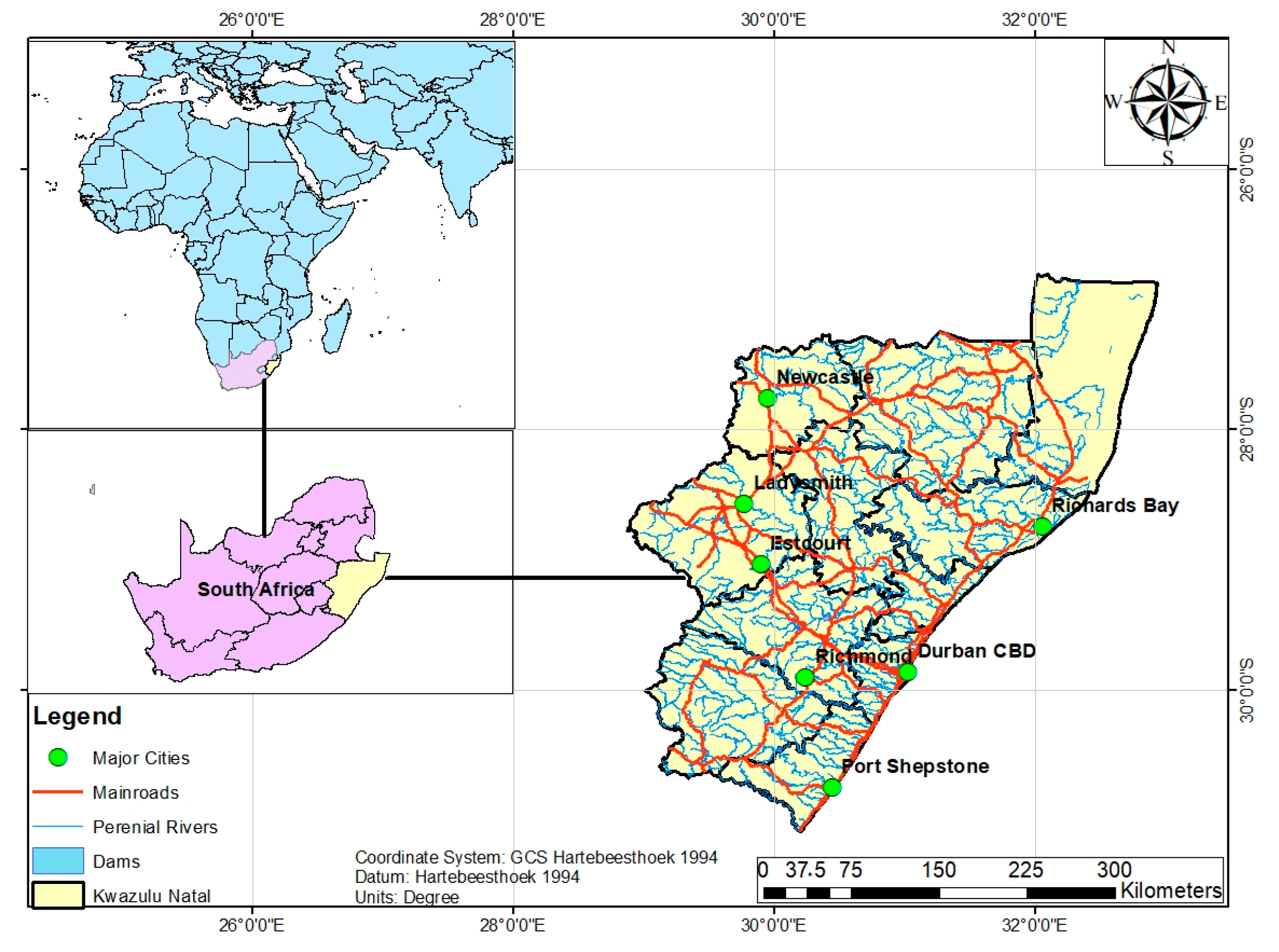
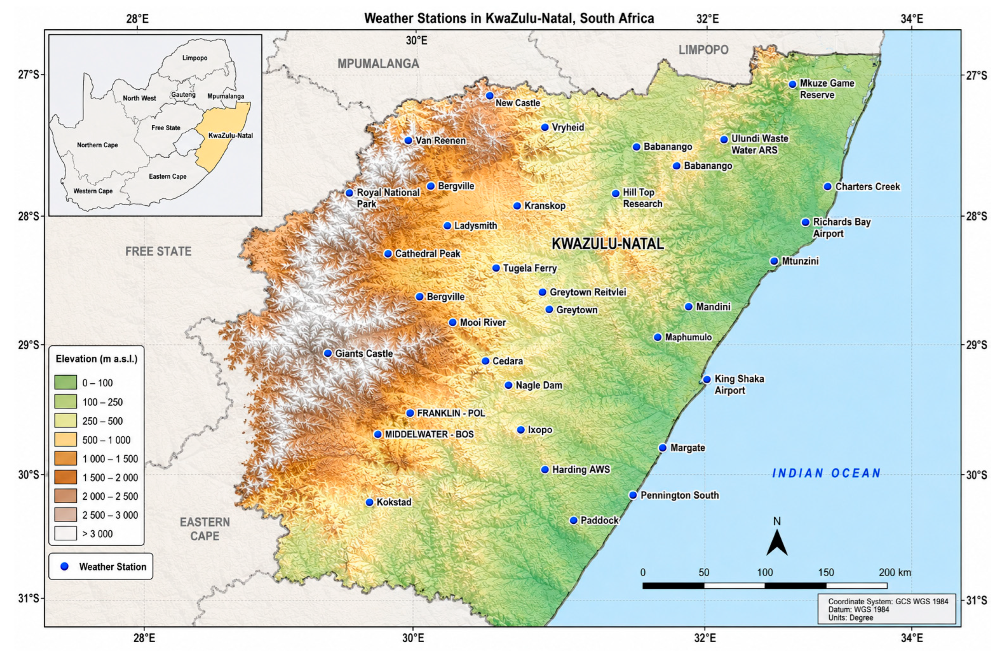
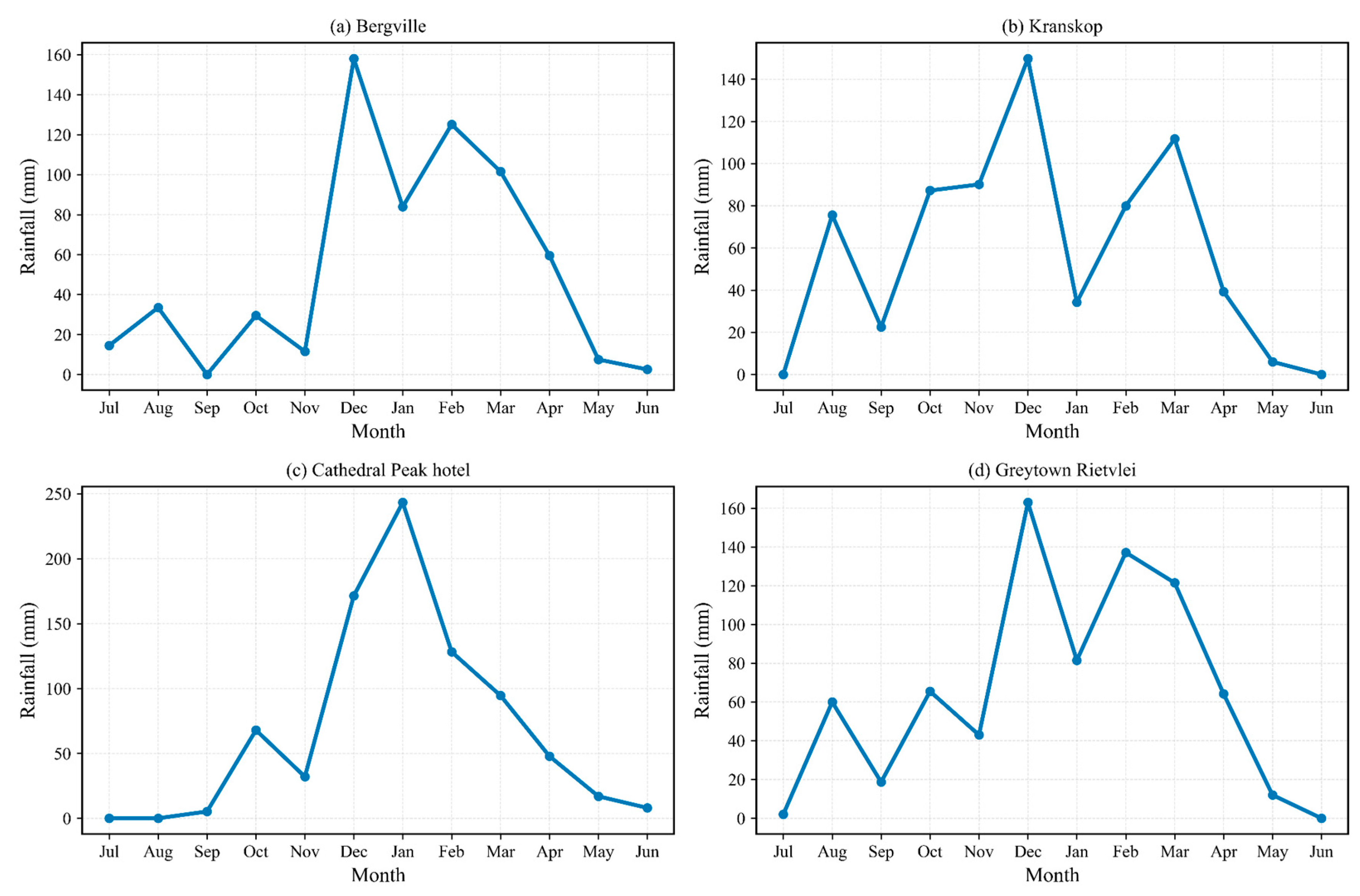
The study focuses on KwaZulu-Natal (KZN), located along the eastern seaboard of South Africa between approximately 26° S–31° S and 29° E–33° E (Figure 1). The region is characterized by complex topography, including the Drakensberg escarpment to the west and a low-lying coastal plain to the east, which strongly influences rainfall distribution and extreme precipitation processes. KwaZulu-Natal lies within the summer rainfall zone of southern Africa and is influenced by moisture transport from the southwest Indian Ocean and the Mozambique Channel. South Africa is predominantly a semi-arid region, with annual rainfall surpassing 600 mm primarily in the eastern areas [10]. Drakensberg mountain range in KwaZulu-Natal constitutes a section of the primary escarpment in the southern region of Africa, extending along the subcontinent’s passive margin. Typically reaching elevations of 2800–3000 m, this escarpment acts as a watershed, delineating the interior basins of Lesotho from the shorter and more precipitous river basins in KwaZulu-Natal. While other areas in South Africa experience summer precipitation, the quantity and timing of peak rainfall are distinct [11]. Western Cape and Northern Cape predominantly receive rain during the winter season, whereas the Cape South Coast is characterized by year-round precipitation [2,12,13]. Despite notable disparities in the annual rainfall patterns, much of the region is subject to rainfall during the austral summer months (December–February), as opposed to the Western Cape Province, which predominantly receives rainfall during the austral winter months (June–August).Bergville and Kranskop stations, as well as Cathedral Peak and Greytown Rietvlei stations, see an earlier peak in rainfall during October (Figure 4a,b). At Cathedral Peak, situated in the Drakensberg, peak rainfall reaches up to 243.3 mm per month in October (Figure 2). During the dry season, the region gets less than 2 mm of rain. However, the summer months are marked by numerous days of heavy downpours.

Moist air moving from the warm Indian Ocean toward the land rises over higher terrain, leading to orographic lifting, which enhances convection, increases atmospheric moisture, soil moisture, and supports dense vegetation [14]. Subsequently, conditions for rainfall are enhanced based on the combination of ideal thermodynamic processes. The province receives an average annual rainfall of more than 800 mm. Large-scale atmospheric systems play an important role in rainfall variability over KwaZulu-Natal, particularly through their influence on low-level moisture conditions [15]. In addition, anomalously strong southerly airflow is characteristic of wetter early-summer conditions (October–December), whereas warmer-than-normal sea surface temperatures east of KwaZulu-Natal contribute to enhanced rainfall during the late-summer period (January–March).

2.2. Reanalysis and Gridded Datasets

Atmospheric circulation fields were obtained from the NCEP/NCAR Reanalysis-2 dataset [16] and the ERA5 reanalysis produced by the European Centre for Medium-Range Weather Forecasts. Data processing and analysis were conducted using Python 3.12 (Python Software Foundation, Wilmington, DE, USA). ArcGIS Pro version 3.4.3 (Esri, Redlands, CA, USA) was used for spatial processing and map production. ERA5 data were used at a spatial resolution of 0.25° × 0.25°, while NCEP/NCAR fields were obtained at 2.5° × 2.5° resolution to maintain consistency with established synoptic climatology studies [17]. Six-hourly reanalysis data were averaged to daily means to correspond with daily rainfall observations. Variables extracted included sea level pressure, geopotential height at 500 hPa, air temperature at 200 hPa, wind vectors at 850 hPa and 500 hPa, relative humidity at 500 hPa and 300 hPa, vertical velocity (omega) at 500 hPa, and outgoing longwave radiation (OLR). Lower-level moisture transport was primarily assessed using the 850 hPa wind fields, while the 500 hPa wind fields were used mainly to characterize mid-tropospheric circulation and steering flow; therefore, 500 hPa winds were not interpreted alone as a direct measure of vertically integrated moisture transport. Daily anomalies were computed by subtracting the 1990–2020 climatological mean from event-specific fields. These variables were also used to identify the complete population of COL systems during 1990–2020 independently of the observed rainfall response. Rainfall observations were subsequently matched to the objectively identified COL events for event classification and impact assessment.

2.3. Weather Stations

Daily rainfall observations from multiple weather stations across KwaZulu-Natal were obtained from the South African Weather Service (SAWS) for the period 1990–2020. Stations were selected to represent a range of elevations, including coastal lowland areas and the central midlands, and only stations with at least 80–95% data completeness over the study period were included. Rainfall observations were collected simultaneously across all stations, enabling consistent spatial and temporal comparison. The South African Weather Service, a member of the WMO, has been responsible for national weather and climate data collection since 1936 and maintains one of the most comprehensive observational networks in the Southern Hemisphere. Elevation influences surface runoff, drainage efficiency, and orographic enhancement of precipitation, with low-lying areas generally exhibiting higher flood susceptibility than elevated regions [17]. Rainfall observations from 34 station records distributed across KwaZulu-Natal were compiled to characterize the spatial and temporal variability of rainfall across the study area (Figure 2). The stations encompass coastal, inland, midlands, and escarpment environments and have varying elevations and data availability (

Table 1. Weather station details over KwaZulu-Natal.

No	Station Name	Latitude	Longitude	Altitude	Availability
1	Bergville	−28.731	29.354	1145	94.88%
2	Kranskop	−28.5756	30.5145	1140	94.32%
3	Cathedral Peak	−28.9476	29.2071	1466	95.18%
4	Giants Castle	−29.2641	29.5223	1759	95.18%
5	Greytown Reitvlei	−29.1156	30.1835	1371	81.00%
6	King Shaka Airport	−29.6108	31.1239	91	92.50%
7	Margate	−30.5131	30.2025	163	99.90%
8	Paddock	−30.7544	30.2577	506	87.70%
9	Van Reenen	−28.3789	29.3853	1683	94.70%
10	Mtunzini	−28.9474	31.7079	41	95.40%
11	Royal National Park	−28.6858	28.9542	1392	97.50%
12	Richards Bay Airport	−28.7378	32.0934	36	94.40%
13	Mkuze Game Reserve	−27.598	32.217	319	95.90%
14	Charters Creek	−28.1978	32.4142	20	97.00%
15	Tugela Ferry	−28.748	30.443	559	95.20%
16	Greytown	−29.083	30.603	1050	98.50%
17	Cedara	−29.541	30.265	1037	99.30%
18	Mooi River	−29.218	30.002	1100	98.20%
19	Nagle Dam	−29.583	30.622	409	99.20%
20	Ulundi Wastewater ARS	−28.347	31.429	540	90.80%
21	Mandini	−29.158	31.402	100	95.90%
22	Ixopo	−30.152	30.074	986	97.30%
23	Kokstad	−30.502	29.394	1316	94.70%
24	Pennington South	−30.399	30.685	70	96.20%
25	FRANKLIN-POL	−30.3175	29.4508	1150	98.00%
26	MIDDELWATER-BOS	−30.3419	29.8706	1400	90.80%
27	Hill Top Research	−28.0688	32.0343	100	97.30%
28	Ladysmith	−28.575	29.7500	1010	95.00%
29	Kranskop Prison	−28.9650	30.8620	1150	94.30%
30	Babanango	−28.3640	31.2060	1000	96.10%
31	New Castle	−27.7685	29.9771	1194	94.70%
32	Vryheid	−27.7773	30.7961	1170	98.00%
33	Harding AWS	−29.8856	29.8856	1050	97.20%
34	Maphumulo	−29.1608	31.0690	650	94.60%

). For the formal long-term trend analysis, four representative stations (Bergville, Kranskop, Cathedral Peak, and Greytown Rietvlei) with sufficiently consistent records were selected for application of the Mann–Kendall test and Sen’s slope estimator. Trend analyses using the Mann–Kendall test and Sen’s slope estimator have been widely applied to assess changes in rainfall and runoff patterns in southern African catchments, including the lower Mzingwane Catchment in Zimbabwe, where rainfall generally showed declining but statistically insignificant trends, while runoff trends varied between stations [16]. The Global Precipitation Climatology Project (GPCP) Version 2.3 rainfall dataset was also employed in this study. This dataset combines rainfall observations from several sources, including satellite and surface-based measurements. It integrates local rain-gauge observations with precipitation estimates derived from passive microwave sensors on polar-orbiting meteorological satellites and infrared (IR) sensors aboard geostationary satellites. The dataset provides monthly precipitation estimates at a spatial resolution of 2.5° × 2.5° for the period 1979–2013. The rain-gauge observations incorporated into GPCP are obtained from the Global Precipitation Climatology Centre Version 7 GPCCv7 [18].

2.4. Spatiotemporal and Statistical Analysis

For the event-based extreme-rainfall analysis, a fixed threshold of ≥50 mm in 24 h was used to classify heavy-rainfall events at the station level. This threshold was applied consistently across the study period and was not derived from seasonal rainfall percentiles. The broad-scale rainfall pattern was assessed using GPCP, while SAWS observations were used to quantify station-level spatial variability. Mean DJF rainfall was calculated for each station and correlated with longitude and latitude using Pearson and Spearman correlation coefficients. The relationship between rainfall and ENSO was assessed using the NOAA Niño 3.4 SST anomaly index. Niño 3.4 is widely used for monitoring ENSO and has been shown to provide a robust measure of ENSO-related climate variability, including rainfall variability over southern Africa [19,20]. Station rainfall anomalies were correlated with Niño 3.4 anomalies at monthly and seasonal scales, with DJF treated as the primary season because of the dominance of summer rainfall in KZN. A regional standardized DJF rainfall index was also developed from the SAWS stations to assess the overall ENSO signal. Statistical significance was assessed at p < 0.05, and the Benjamini–Hochberg false-discovery-rate correction was applied to account for multiple station-level comparisons.

2.5. Composite and Anomaly Analysis

Composite analysis was employed to examine mean atmospheric circulation patterns associated with extreme rainfall events, particularly during La Niña and El Niño phases. Diagnostic fields included sea-level pressure anomalies, geopotential height anomalies, wind vector anomalies, relative humidity, vertical velocity (omega), and OLR. These methods are well established in synoptic climatology and were applied consistently across all case studies to ensure comparability. Composite analysis was conducted for extreme rainfall days, ENSO phase subsets, COL events, and selected case studies. Atmospheric anomalies were computed relative to the 1990–2020 climatological mean. Composite anomaly fields were interpreted as diagnostic descriptions of the mean atmospheric conditions associated with the selected rainfall events and climate-phase subsets. The magnitude and spatial structure of the anomalies were examined descriptively rather than subjected to formal pixel-wise statistical significance testing. Area-averaged diagnostics, including omega and relative humidity, were calculated over predefined regional domains encompassing the eastern escarpment and coastal KwaZulu-Natal to quantify vertical motion intensity and atmospheric moisture conditions during peak rainfall events. For COL analysis, composites and event diagnostics were distinguished between the complete population of identified COLs and the subset associated with extreme rainfall (≥50 mm day⁻¹). This separation was used to examine whether the atmospheric conditions associated with high-rainfall COLs differed from those associated with COLs producing lower rainfall.

2.6. Case Study Approach

A case study methodology was applied to selected tropical cyclones, tropical-temperate troughs, and cut-off low events to examine their synoptic structure, evolution, and rainfall impacts. Following the independent identification of the complete COL population, selected high-rainfall COL events were chosen for detailed case-study analysis. Case-study selection was based on rainfall magnitude and representativeness of the atmospheric structure and was therefore performed after, rather than during, the initial COL identification. Daily reanalysis fields, satellite-derived cloud imagery, and surface rainfall observations were jointly analyzed to assess moisture transport, uplift mechanisms, and system persistence. This approach allows for detailed diagnosis of high-impact events that are not fully captured by climatological averages.

2.7. Data Availability

Meteorological reanalysis datasets are obtained through a collaborative initiative between the National Centers for Environmental Prediction (NCEP), formerly the National Meteorological Center (NMC), and the National Center for Atmospheric Research (NCAR). This partnership, designated as NCEP/NCAR, originated from the Climate Data Assimilation System project. The NCEP/NCAR effort employs continuously updated gridded datasets that depict the atmospheric conditions of the Earth, amalgamating observations and outputs from numerical weather prediction (NWP) models since 1948 [17]. The datasets are provided at 6-hourly intervals, specifically at 00:00 UTC, 06:00 Z, 12:00 Z, and 18:00 Z. The NCEP/NCAR Reanalysis datasets used in this study include outgoing long-wave radiation (a), geopotential height (b), wind vectors (c), relative humidity (d), and omega (e). According to [7], these datasets come from combining data from sources such as surface observations, balloon measurements, aircraft, ships, radiosondes, and satellites. These data go through quality checks before being made available online. The information comes from the NCEP/NCAR Reanalysis-2 (R-2) [21], which features 17 vertical pressure levels ranging from 1000 to 10 hPa. This newer version has fixed known issues from the earlier NCEP Reanalysis 1 (R-1), leading to improved reanalyses for different parameters [21].

Missing data within the daily rainfall records were addressed using within-station temporal interpolation techniques. Although several methods exist for handling data gaps, including regression-based approaches and spatial extrapolation from neighbouring stations [22], this study applied an interpolation method based on temporal information from the same station, using rainfall values from days preceding and following the missing observations. This approach is well suited for short data gaps and has been shown to produce reliable estimates when missing periods span one or a few consecutive days [23]. The choice of this method ensured data continuity while minimizing distortion of extreme rainfall characteristics.

3. Results

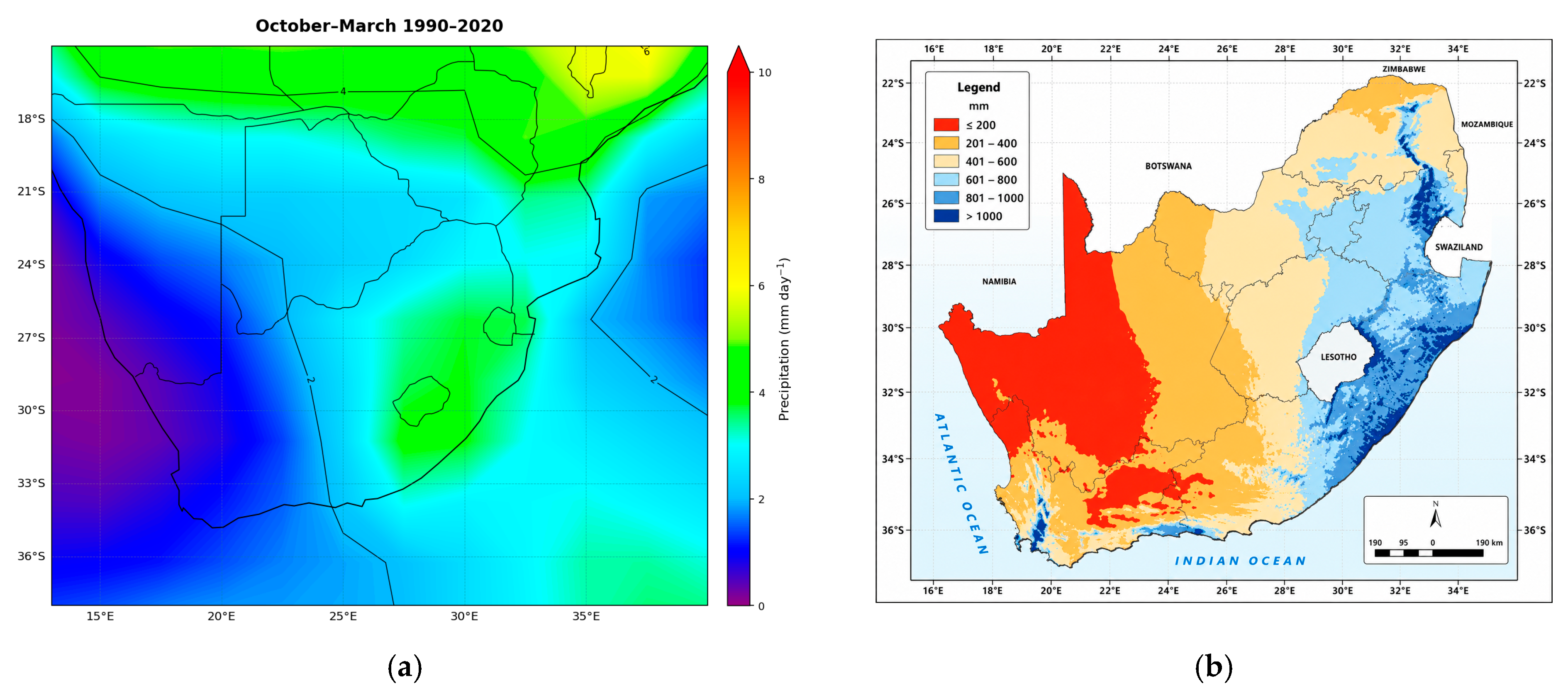
The results of this study demonstrate that extreme rainfall in the region is controlled by multiscale interactions involving large-scale climate variability, synoptic-scale weather systems, and regional topographic controls. The pronounced west–east rainfall gradient identified across the province is consistent with earlier climatological studies and reflects the combined influence of moisture transport from the southwest Indian Ocean and orographic enhancement along the Drakensberg escarpment (Figure 3a). These spatial patterns highlight the heightened vulnerability of eastern and escarpment regions to extreme rainfall and flooding.

3.1. Spatiotemporal Variability of Rainfall

GPCP spatial distribution presented in Figure 3a reveals a pronounced concentration of higher precipitation over the eastern parts of South Africa and adjacent Indian Ocean regions during the summer season (October to March). A distinct rainfall core is evident over KwaZulu-Natal (KZN) and the offshore region, where values exceed approximately 5–6 mm/day, indicating a strong influence of oceanic moisture influx. In contrast, markedly lower rainfall values (below 4–4.5 mm/day) are observed toward the western interior, extending into arid regions of South Africa and Namibia. These GPCP fields indicate a broad west–east rainfall gradient, with precipitation generally increasing toward the eastern coastline. Given the 2.5° × 2.5° spatial resolution of GPCP, this gradient is interpreted as a broad regional-scale precipitation pattern rather than a station-resolved spatial field. The gradient is spatially consistent and highlights the dominance of moisture-bearing systems originating from the southwest Indian Ocean. The localized maximum over eastern South Africa further suggests the role of coastal and topographic enhancement in intensifying rainfall in this region. In Figure 3b, the mean annual precipitation distribution over South Africa reinforces this pattern at a national scale. The eastern escarpment and coastal belt, particularly across KZN, exhibit significantly higher rainfall totals, while the western and southwestern regions remain comparatively dry.

The transition zone between these regions is gradual, reflecting a range rather than an abrupt boundary in rainfall distribution. Temporal variability is also implied in Figure 3a through the spatial pattern of rainfall trends, where regions of enhanced rainfall correspond with areas of persistent summer precipitation maxima. The consistency of higher rainfall over the eastern regions across the 31-year period suggests relative stability in the spatial pattern, despite potential interannual variability. The resolution of the GPCP data highlights the importance of orographic effects (Figure 3a). The eastern escarpment of the Drakensberg promotes the lifting of moist air from the Indian Ocean, influenced by a high-pressure system off the coast of KwaZulu-Natal. While these weather extremes can cause significant damage to infrastructure and result in loss of life, their impacts often extend to agriculture and human health. A recent study by [24] found that flooding is the most frequently occurring weather-related extreme event in South Africa, highlighting the country’s vulnerability to flood-related impacts. There is significant variability in extreme wet seasons over central KwaZulu-Natal, which indicates that this area is particularly prone to severe flooding events during the summer months (Figure 3a). The flood season is often linked to frequent heavy rain spells, making the region more susceptible to floods.

3.1.1. Annual Cycle and Intraseasonal Rainfall Variability

As illustrated in Figure 4, the spatial distribution of rainfall throughout the study area exhibits a markedly seasonal pattern, with 70–80% of the precipitation occurring during the austral summer months from October to March. During this period, monthly rainfall amounts can exceed 100 mm. The onset of rainfall may commence earlier in October, and in exceptional situations, the rainy season may extend into April. On intraseasonal timescales, the rainy season in southern Africa is distinguished by alternating periods of wet and dry conditions [25].

3.1.2. Interannual Variability

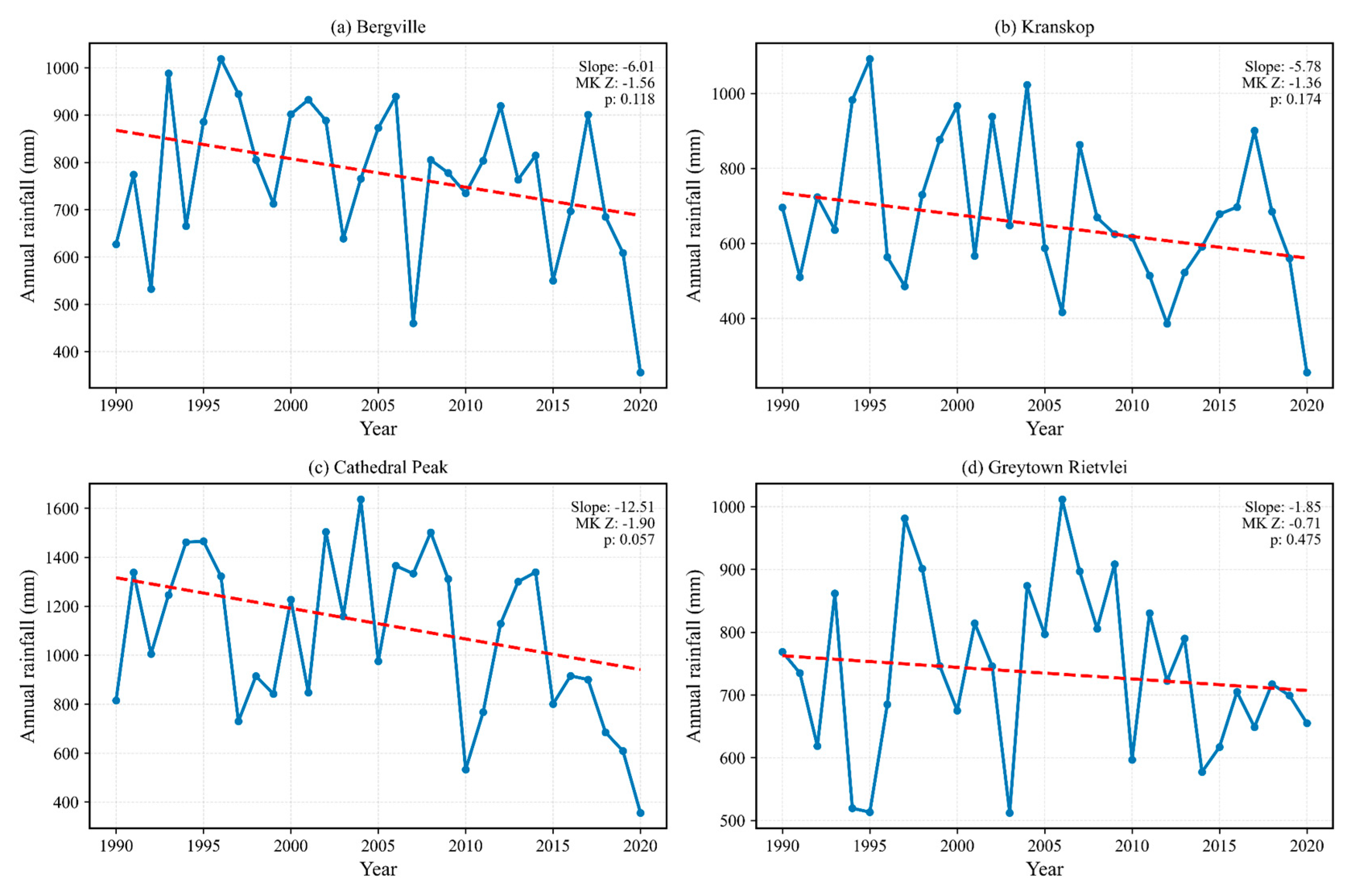
Trend analysis of annual rainfall totals was conducted for four representative stations across KwaZulu-Natal using the Mann–Kendall test and Sen’s slope estimator (Figure 5). All four stations exhibited negative Sen’s slope estimates over the 1990–2020 period, indicating a downward direction in the estimated linear change in annual rainfall. Bergville and Kranskop had Sen’s slope estimates of −6.01 and −5.78 mm yr⁻¹, respectively, while Greytown Rietvlei recorded −1.85 mm yr⁻¹. Cathedral Peak exhibited the largest negative slope of −12.51 mm yr⁻¹. However, the Mann–Kendall tests did not indicate statistically significant monotonic trends at the 95% confidence level. The p-values were 0.118 for Bergville, 0.174 for Kranskop, 0.475 for Greytown Rietvlei, and 0.057 for Cathedral Peak. Although the Cathedral Peak result approached the 0.05 significance threshold, it remained statistically non-significant at the predefined 95% confidence level. Therefore, the negative Sen’s slope estimates are interpreted as the direction and magnitude of the estimated changes rather than as evidence of a statistically established decreasing rainfall trend.

The results consequently indicate that the long-term trend in annual rainfall over the four stations is inconclusive for the 1990–2020 period. The absence of statistically significant Mann–Kendall trends, together with the substantial year-to-year variability evident in Figure 4, suggests that interannual fluctuations are more pronounced than any detectable monotonic change in annual rainfall totals during the study period. The pronounced wet and dry years further demonstrate the variability of annual rainfall across the study region. Accordingly, the analysis does not provide sufficient statistical evidence to conclude that KwaZulu-Natal experienced a significant decline in annual rainfall during 1990–2020. The observed negative slope estimates may indicate a possible downward tendency at the selected stations, particularly at Cathedral Peak, but this interpretation requires further investigation using longer records and additional stations before a regional drying trend can be established. Extreme rainfall intensity and frequency can exhibit substantial interannual variability and periodic wet–dry fluctuations, with the persistence of future trends remaining uncertain [26].

The negative Sen’s slope estimates observed at the four stations indicate a consistent downward direction in the estimated annual rainfall changes; however, the lack of statistical significance means that these estimates cannot be interpreted as evidence of a regional rainfall decline. The large year-to-year fluctuations shown in Figure 5 indicate substantial interannual variability, including pronounced wet and dry years. Such variability may reflect the influence of large-scale climate variability and episodic synoptic-scale rainfall systems, which are examined in subsequent sections. The present trend analysis therefore provides no conclusive evidence of a monotonic long-term decrease in annual rainfall over the selected stations during 1990–2020.

3.2. Large-Scale Climate Drivers of Rainfall Variability

To better understand the mechanisms responsible for the observed interannual rainfall variability across KwaZulu-Natal in Figure 5, large-scale climate drivers were investigated. Previous studies have shown that rainfall variability over southern Africa is strongly influenced by coupled ocean-atmosphere interactions, particularly the El Niño–Southern Oscillation (ENSO), which modulates regional moisture transport, convection, and atmospheric circulation patterns. The El Niño–Southern Oscillation (ENSO) was characterized using both the Southern Oscillation Index (SOI), representing the atmospheric component of ENSO, and the Niño 3.4 sea-surface temperature anomaly index, representing its oceanic component. Niño 3.4 is widely used for monitoring ENSO and has been shown to provide a robust measure of ENSO-related climate variability, including rainfall variability over southern Africa [19,20].

3.2.1. Southern Oscillation and Seasonal Rainfall

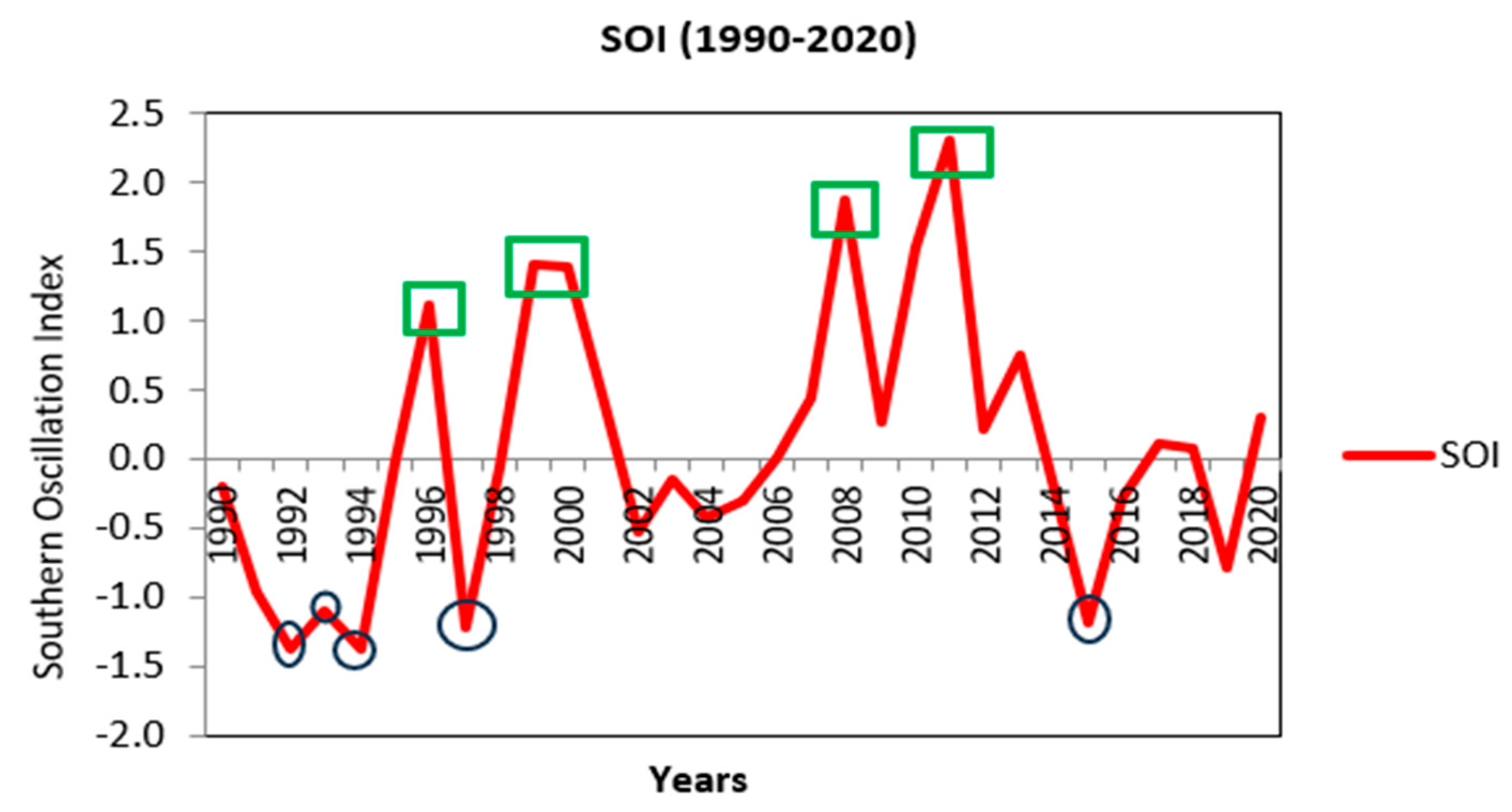
The Southern Oscillation influences the variability of precipitation in the Southern Hemisphere and is associated with the El Niño/La Niña phenomena [20]. The Southern Oscillation Index (SOI) is an atmospheric indicator of ENSO calculated from the standardized anomaly of the mean sea-level pressure difference between Tahiti and Darwin [27]. The time series analysis of the SOI from 1990 to 2020 delineates oscillations between positive phases (La Niña) and negative phases (El Niño), including occasional intervals of neutral conditions (Figure 5). In this study, the identification of El Niño and La Niña phenomena were performed utilizing SOI and the Niño 3.4 index (Figure 6). Correlation analysis was performed between seasonal rainfall totals and the SOI and Niño 3.4 indices for DJF, MAM, JJA, and SON, including contemporaneous (lag 0) and 1–3-month lagged relationships (

Table 2. Seasonal and lagged correlations between the regional rainfall index and ENSO indices (1990–2020).

Seasons	Lag_Months	ENSO_Index	Pearson_r	p_Value	n
DJF	0	Niño 3.4	−0.4473	0.0132	30
DJF	0	SOI	0.2377	0.2059	30
DJF	1	Niño 3.4	−0.4513	0.0123	30
DJF	1	SOI	0.2642	0.1583	30
DJF	2	Niño 3.4	−0.4420	0.0145	30
DJF	2	SOI	0.2382	0.2049	30
DJF	3	Niño 3.4	−0.4187	0.0213	30
DJF	3	SOI	0.2804	0.1334	30
MAM	0	Niño 3.4	−0.1507	0.4185	31
MAM	0	SOI	0.1049	0.5745	31
MAM	1	Niño 3.4	−0.1626	0.3821	31
MAM	1	SOI	0.0998	0.5932	31
MAM	2	Niño 3.4	−0.1707	0.3586	31
MAM	2	SOI	0.1434	0.4416	31
MAM	3	Niño 3.4	−0.1709	0.3665	30
MAM	3	SOI	0.1539	0.4168	30
JJA	0	Niño 3.4	0.3249	0.0745	31
JJA	0	SOI	−0.1838	0.3223	31
JJA	1	Niño 3.4	0.2254	0.2228	31
JJA	1	SOI	−0.1619	0.3842	31
JJA	2	Niño 3.4	0.0742	0.6914	31
JJA	2	SOI	−0.1173	0.5298	31
JJA	3	Niño 3.4	−0.0688	0.7132	31
JJA	3	SOI	−0.0158	0.9327	31
SON	0	Niño 3.4	−0.1736	0.3503	31
SON	0	SOI	0.1578	0.3964	31
SON	1	Niño 3.4	−0.1256	0.5007	31
SON	1	SOI	0.0910	0.6265	31
SON	2	Niño 3.4	−0.0956	0.6090	31
SON	2	SOI	0.0631	0.7360	31
SON	3	Niño 3.4	−0.1083	0.5619	31
SON	3	SOI	0.0401	0.8303	31

). The relationship between ENSO variability and regional rainfall varied by season and lag. The strongest and statistically significant relationships occurred during DJF between the regional rainfall index and Niño 3.4. Significant negative correlations were observed at lags of 0 months (r = −0.447, p = 0.013), 1 month (r = −0.451, p = 0.012), 2 months (r = −0.442, p = 0.014), and 3 months (r = −0.419, p = 0.021). These results indicate that positive Niño 3.4 anomalies were consistently associated with reduced regional summer rainfall across the study area. In contrast, correlations during MAM, JJA, and SON were not statistically significant at the 95% confidence level. The SOI correlations were also not statistically significant for any season or lag. The results therefore indicate that the ENSO-rainfall relationship is strongest and most consistent during the austral summer rainfall season.

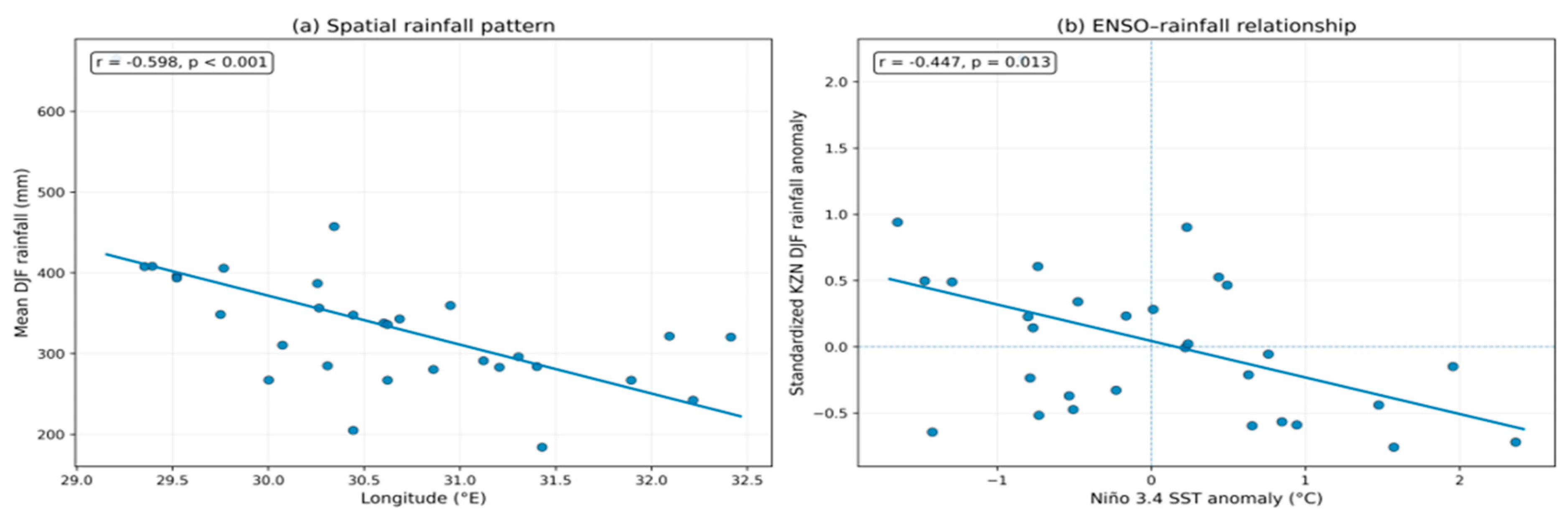
Figure 6 shows the annual Southern Oscillation Index (SOI) during 1990–2020 and highlights the major positive and negative SOI phases identified during the study period. Positive SOI values are generally associated with La Niña conditions, whereas negative values are associated with El Niño conditions. Based on the threshold adopted in this study (SOI ≥ 1 for La Niña and SOI ≤ −1 for El Niño), four major La Niña periods were identified during the study period and 5 major El Niño periods. However, the frequency of SOI phases alone does not establish a direct relationship with extreme flooding. Therefore, the identified La Niña periods were further examined in conjunction with observed rainfall and other relevant climate drivers to assess their contribution to extreme precipitation and flooding over KwaZulu-Natal. The spatial distribution of observed summer rainfall was performed using the SAWS stations included in the study dataset. Mean December–January–February (DJF) rainfall showed a significant longitudinal spatial organization across the station network (Pearson r = −0.598, p < 0.001; Spearman ρ = −0.666, p < 0.001) (Table 2). Rainfall generally decreased towards the eastern longitudes, although substantial station-to-station departures from the fitted relationship were evident. These local departures are consistent with the complex topographic and coastal influences on rainfall across KwaZulu-Natal. The station observations therefore support a broad-scale spatial structure while also demonstrating considerable local variability. The relationship between ENSO and summer rainfall was subsequently evaluated using the Niño 3.4 SST anomaly (Figure 7a,b). Of the 25 stations with at least 10 complete DJF seasons, 22 (88%) showed negative Pearson correlations between DJF rainfall anomalies and Niño 3.4 anomalies, indicating that positive Niño 3.4 conditions were generally associated with reduced summer rainfall (Table 2). Individual station correlations were moderate, with the strongest negative relationships occurring at Paddock (r = −0.436), Empangeni Magistrate (r = −0.414), Kokstad (r = −0.409), and Margate Airport (r = −0.395; p = 0.041) (Figure 7a,b). Because multiple stations were tested, individual p-values were interpreted cautiously; after Benjamini–Hochberg false-discovery-rate correction, no individual station remained significant at q < 0.05. To assess whether the ENSO signal was coherent across the study area rather than controlled by individual stations, standardized DJF rainfall anomalies were averaged across the station network for each season. The resulting regional rainfall index was significantly and negatively correlated with Niño 3.4 (Pearson r = −0.447, p = 0.013; Spearman ρ = −0.480, p = 0.007). This indicates a coherent regional response, whereby warmer Niño 3.4 conditions tend to coincide with below-normal summer rainfall across the KZN station network. The spatial variability of the ENSO response was tested by relating the station-specific ENSO–rainfall correlations to longitude and latitude. Neither longitude (r = −0.087, p = 0.680) nor latitude (r = −0.079, p = 0.707) was significantly related to the strength of the ENSO-rainfall correlation. Thus, while the observed rainfall field has a significant spatial structure, the ENSO influence does not exhibit a statistically significant west–east or north–south gradient. This distinction suggests that the broad-scale ENSO signal is relatively spatially coherent, whereas the spatial distribution of rainfall itself is strongly modulated by local geographic and orographic factors. Figure 7a,b provides complementary evidence: Figure 7a demonstrates the observed spatial organization of DJF rainfall using the SAWS station network, while Figure 7b demonstrates the regional negative association between Niño 3.4 and standardized DJF rainfall.

3.2.2. Outgoing Longwave Radiation Anomalies

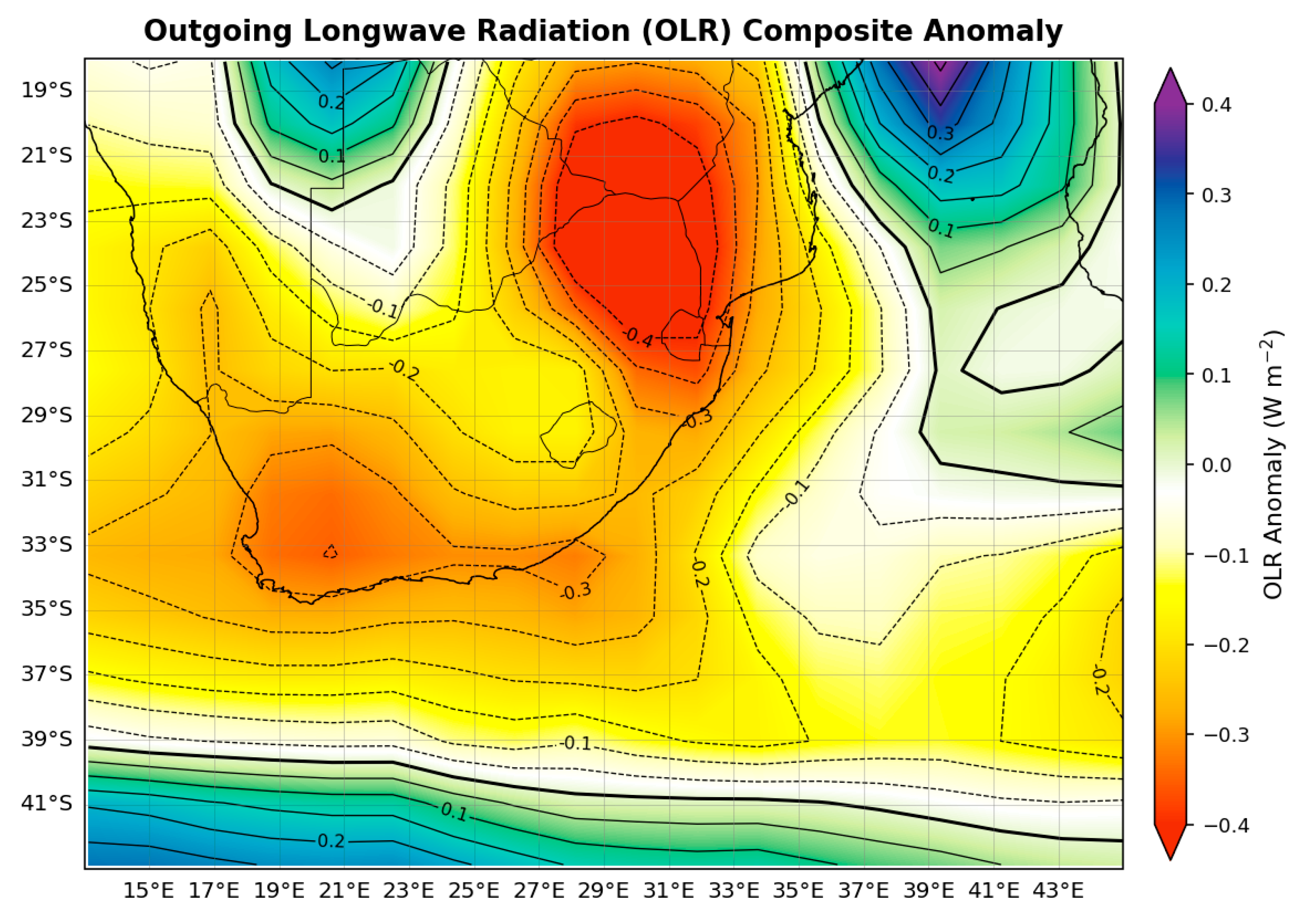
Outgoing longwave radiation (OLR) represents terrestrial radiation emitted to space and is strongly influenced by atmospheric temperature, water vapor, and cloud cover. In the tropics, high OLR values generally indicate relatively clear skies or suppressed convection, whereas low OLR values are associated with high, cold cloud tops characteristic of deep convection and enhanced precipitation [28]. Therefore, in this study, heavy rainfall events may indicate strong negative OLR anomalies, which may result in extreme flooding events. Negative OLR anomalies mainly support this study for extreme flooding events over KwaZulu-Natal. Negative OLR anomalies at 200 hPa were observed over KwaZulu-Natal in late summer (February, March, April) from 1990 to 2020. A detailed analysis of Figure 8 indicates that low OLR values were observed over the coastal areas of KwaZulu-Natal, reflecting enhanced deep convective activity during the late summer season. A detailed analysis of these anomalous years was performed in this study to better understand each case.

3.2.3. Atmospheric Anomalies

An atmospheric anomaly is characterized as the divergence of a quantifiable parameter, such as precipitation or temperature, over a specified temporal duration for a particular geographic region, relative to the long-term average, for instance, a 31-year mean, for that region. Composite analysis was employed for the analysis of anomalies within the mean circulation, often associated with severe flooding events in the study area. Atmospheric anomalies can induce extreme flooding or drought events, which may be connected to oceanic phenomena, such as the spatial fluctuation of Sea Surface Temperature (SST) [29,30]. Circulation anomalies driving extreme flooding events over KwaZulu-Natal are discussed in this section. As shown in Figure 6, the mature years of La Niña events from 1990 to 2020 were associated with tropical cyclones. After a thorough analysis, this study selected cases of tropical cyclones and tropical storms that impacted KwaZulu-Natal from 1990 to 2020.

3.3. Synoptic-Scale Atmospheric Mechanisms

While ENSO and OLR describe the broader climatic conditions favourable for enhanced rainfall, extreme flooding events are ultimately triggered by synoptic-scale weather systems. Therefore, this section examines the contribution of tropical cyclones and associated circulation anomalies to heavy rainfall events over KwaZulu-Natal.

3.3.1. Tropical Cyclone

Tropical cyclones (TCs) are associated with intense winds and heavy rainfall, posing significant hazards. Unpredictable TC paths and extreme rainfall predictions pose notable challenges for traditional weather models [26]. To assess the contribution of tropical systems to extreme rainfall in KwaZulu-Natal, Tropical Cyclone Dineo (February 2017) was selected as a representative case. This event was chosen based on three criteria: The event was selected because of its well-documented regional impacts across southern Africa, the availability of high-resolution observational and satellite datasets, and the substantial socio-economic damage associated with its occurrence. Unlike purely coastal cyclone impacts, Dineo provides a useful example of how decaying tropical systems can still produce significant inland hydrometeorological effects. A historical record indicates that the following tropical cyclones made landfall and influenced southern Africa: Eline (2000), Favio (2007), Dineo (2017), Idai (2019), Kenneth (2019), and Chalane (2020) (

Table 3. Dominant tropical cyclones affecting Southern Africa for 1990–2020. Source: WMO.

Tropical Cyclone	Year	Estimated Damage
Domoina	1984/1985	$100 million USD
Eline	1999/2000	$140 million USD
Favio	2006/2007	$100 million USD
Dineo	2016/2017	$250 million USD
Kenneth	2019/2020	$2 billion USD
Chalane	2019/2020	$50 million USD

). In recent years, countries bordering the Mozambique Channel have experienced several intense and destructive weather events, causing significant social and economic impacts. For example, heavy rainfall associated with Tropical Cyclone Dineo in 2017 resulted in widespread displacement, affecting around 700,000 people, and caused substantial economic losses in Mozambique [31]. The recent tropical cyclones listed below have primarily affected the eastern and coastal regions of the study area after 1990; tropical cyclone Domoina notably impacted the northern part of KwaZulu-Natal.

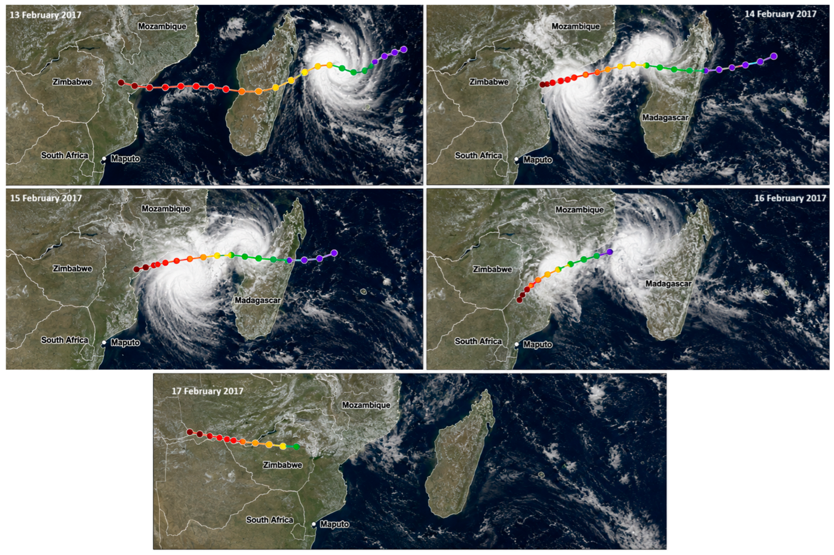
The satellite images show the development and movement of Tropical Cyclone Dineo from 13 to 17 February 2017 (Figure 9). On 13 February, the system was already organized over the Mozambique Channel, and its cloud circulation became more defined as it moved westward. Between 14 and 15 February, Dineo strengthened considerably, with a more compact and well-developed cloud structure as it approached the Mozambican coast. The cyclone reached its strongest stage around 15 February before making landfall in southern Mozambique. After landfall, the system gradually weakened as it moved inland, with the cloud structure becoming less organized on 16 February. By 17 February, the remaining circulation had moved further inland towards Zimbabwe and had lost much of its tropical cyclone structure. By 16 and 17 February, the system weakened further and became a tropical disturbance as it made landfall in South Africa, northeast of KwaZulu-Natal, and later affected Zimbabwe and Botswana. The trajectory of tropical cyclones is strongly influenced by the large-scale environmental steering flow associated with surrounding synoptic-scale pressure systems. In particular, winds in the mid-troposphere, commonly represented by the 500–700 hPa layer, are important in determining tropical cyclone movement. Easterly troughs over the Southwest Indian Ocean (SWIO), notably those that exhibit significant depth, are generally correlated with Pacific La Niña phenomena [32]. During 13–17 February 2017, daily rainfall exceeded 100 mm at several stations, with persistent negative OLR anomalies indicating deep convection. The interaction between the remnant low and large-scale pressure gradients enhanced northeasterly moisture transport into KwaZulu-Natal. This case illustrates that TC-related flooding is often linked to moisture persistence and slow system translation rather than peak wind intensity alone. The cyclone made landfall over Mozambique, South Africa, and Botswana, where its remnants intensified local flooding, leading to extreme weather conditions (Figure 9). As shown in Figure 9, Meteosat satellite images of Tropical Cyclone Dineo between 13 and 15 February 2017 show the extensive cloud cover associated with the storm (Figure 9).

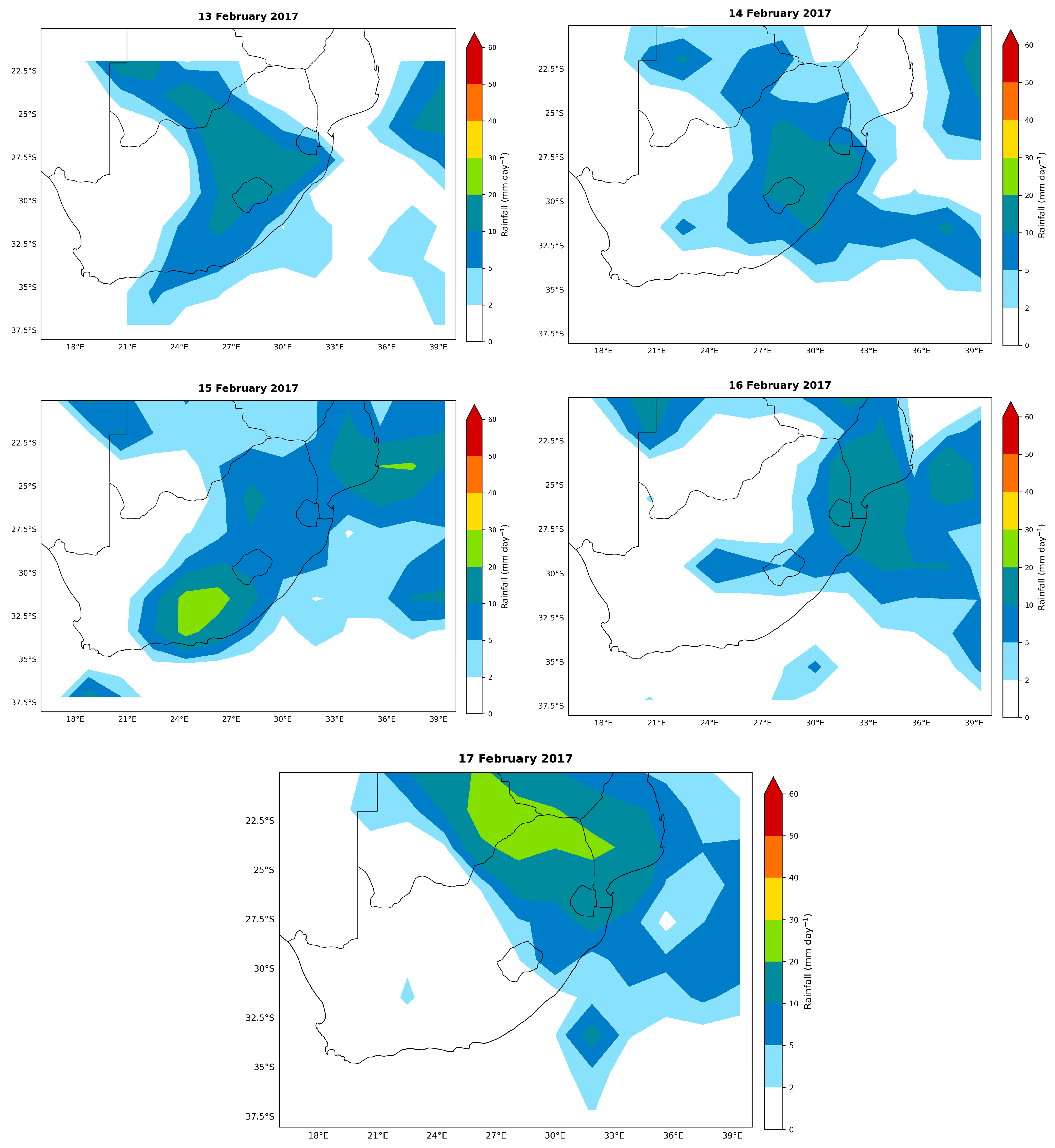
As illustrated in Figure 9, on 13 February 2017, the mean surface precipitation was below 10 mm while Tropical Cyclone Dineo was positioned over the South Indian Ocean. As the system advanced towards the mainland on 14 February 2017, the study region experienced more than 14 mm of rainfall. Extreme flooding events in the northeastern area of KwaZulu-Natal were induced by Tropical Cyclone Dineo, which endured for approximately six days (13–18 February), impacting Mozambique, South Africa, and Botswana. Tropical Cyclone Dineo made landfall in southern Mozambique (depicted in Figure 9), where over 22 mm of precipitation was recorded. Tropical cyclones originating in the SWIO and making landfall in Mozambique typically diminish in intensity as they advance westward into the interior of southern Africa. Upon traversing terrestrial regions, these systems generally downgrade to lower-intensity meteorological phenomena, such as former tropical cyclones or remnant lows, owing to the depletion of moisture and energy. Predominantly, these attenuated systems tend to dissipate upon reaching nations like Botswana [33]. Nevertheless, despite the reduction in their potency, these systems are still capable of engendering considerable precipitation inland, significantly contributing to the overall seasonal rainfall of the affected territory [33]. The cyclone’s slow movement and sustained heavy rainfall contributed to prolonged flooding and heightened the risk of landslides in affected inland and coastal areas of KwaZulu-Natal. Other areas affected included Dube Village, Port Durnford, and eNseleni. Several individuals were rescued after their vehicles were swept away. The surface precipitation rate composite mean shows a clear spatiotemporal evolution of rainfall associated with Tropical Cyclone Dineo from 13 to 17 February 2017, with precipitation initially concentrated over southern Mozambique and the Mozambique Channel before shifting progressively inland and south-westward (Figure 10). The highest composite mean precipitation rates, reaching approximately 20–30 mm day⁻¹, are concentrated around southeastern Mozambique and northeastern South Africa, while lower rates occur farther from the cyclone-affected region (Figure 10). By 17 February 2017, the precipitation maximum became more organized over southeastern southern Africa, indicating the progressive south-westward movement of the cyclone and its associated rainfall system.

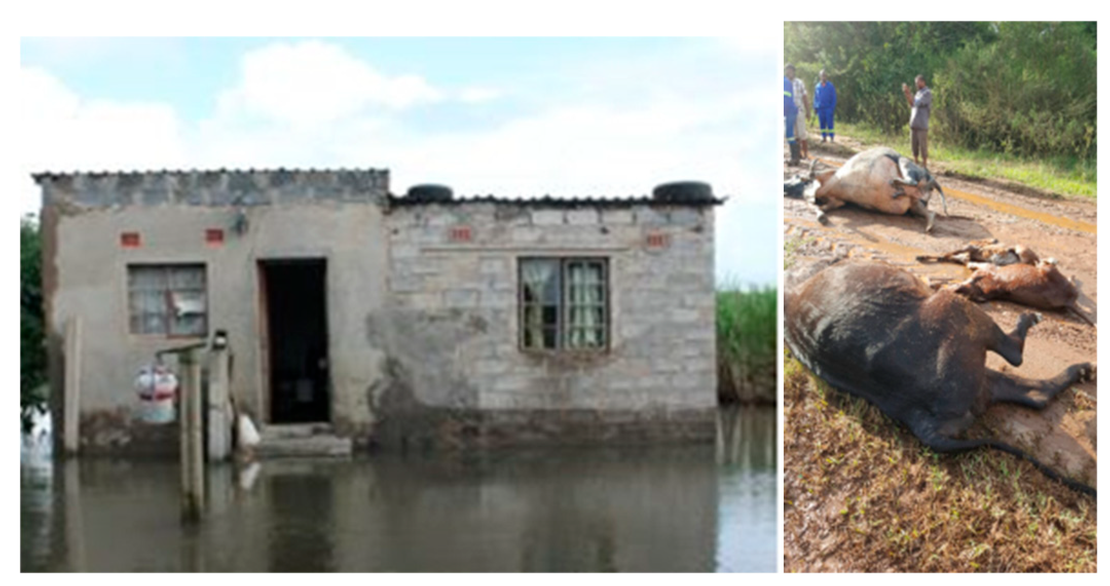
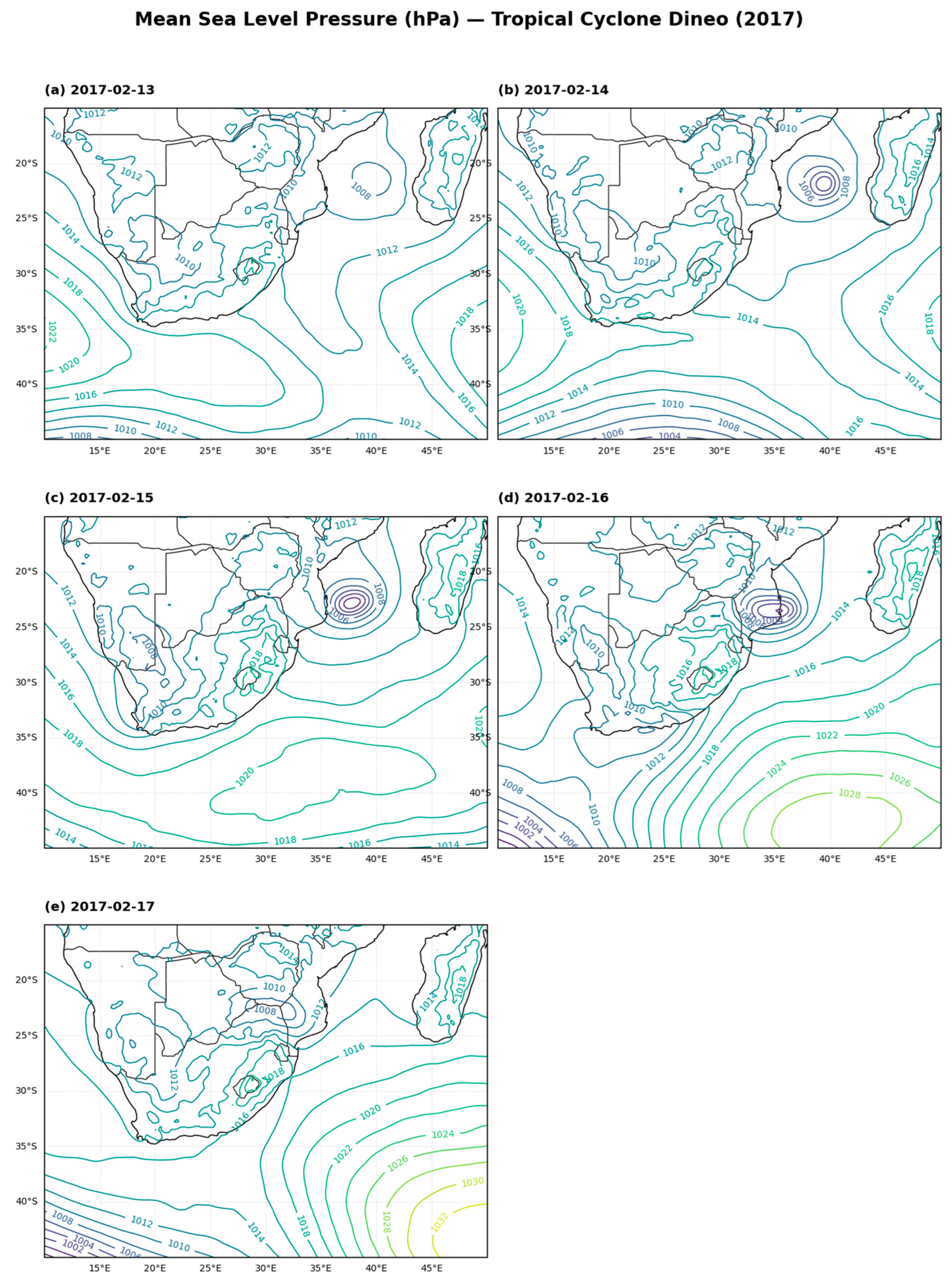
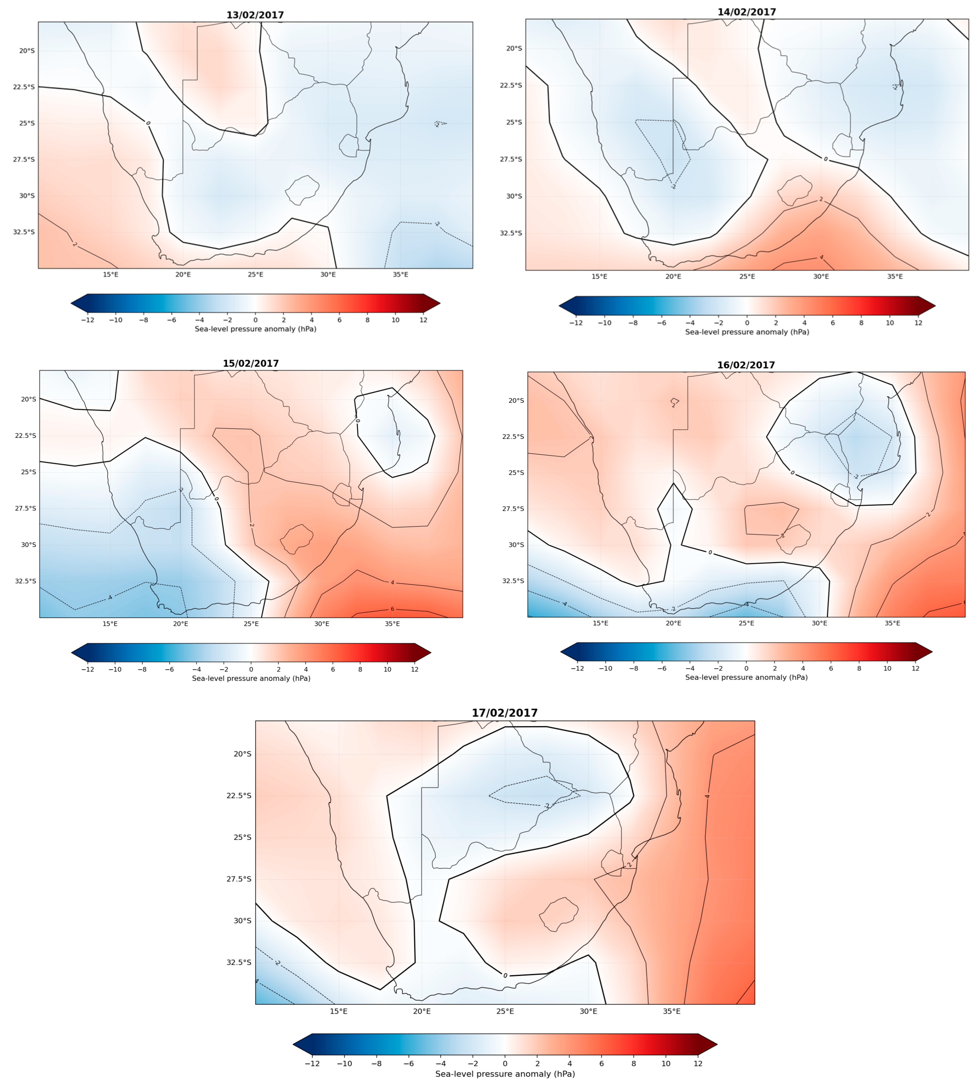
The mean sea level pressure indicates that a continuous high-pressure system prevailed over southern Africa throughout the duration of Tropical Cyclone Dineo’s occurrence (Figure 11). High-pressure systems are crucial in influencing the trajectory of tropical cyclones, as they influence the large-scale wind patterns at mid-tropospheric levels, particularly around the 500 and 700 hPa pressure levels. These steering winds are crucial in determining the trajectory of cyclones, including Dineo, which lasted for at least five days. It is evident from the images the extent of Tropical Cyclone Dineo affected the community (Figure 11). In this instance, we focus particularly on the daily mean sea level pressure and the anomalies connected to Tropical Cyclone Dineo as it moved inland from 13 to 17 February 2017 (Figure 12). The anomalies provide critical insight into how the cyclone’s movement was influenced by the surrounding atmospheric conditions, as well as the severity of the impact once it reached land (Figure 12). By 17 February 2017, the satellite imagery clearly depicts the cloud band linked to the remnant low of the cyclone, which had weakened after making landfall.

The images provide valuable insight into the cyclone’s progression, illustrating both its peak intensity and subsequent dissipation as it moved inland (Figure 12a–e) and sea level pressure anomaly (Figure 13). A cloud band is linked with a tropical cyclone and is important in locating the cyclone centre and is associated with heavy rainfall linked with the system [3]. As shown in Figure 12, Tropical Cyclone Dineo advanced from the SWIO and entered the mainland of Mozambique. It traversed over South Africa and Botswana, covering a considerable region (Figure 12). Sea level pressure anomaly (hPa) on 13–17 February 2017 is depicted on Figure 13 with detailed analysis. The northern part of KwaZulu-Natal was also affected by a remnant low that resulted in substantial rainfall. The SWIO and the Mozambique Channel offer favourable conditions for cyclogenesis, especially from mid to late austral summer, which is the peak period for the development of tropical revolving storms [32].

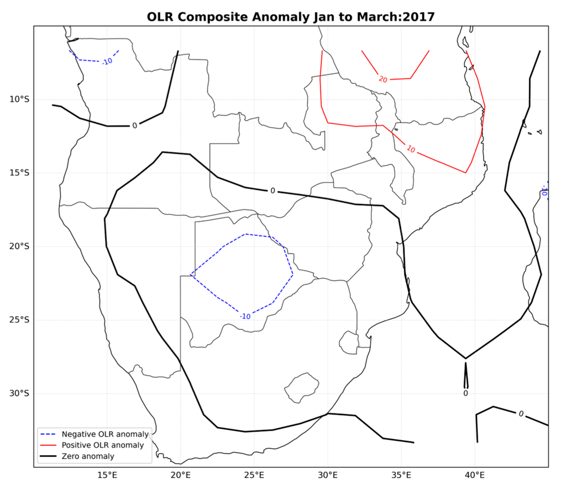
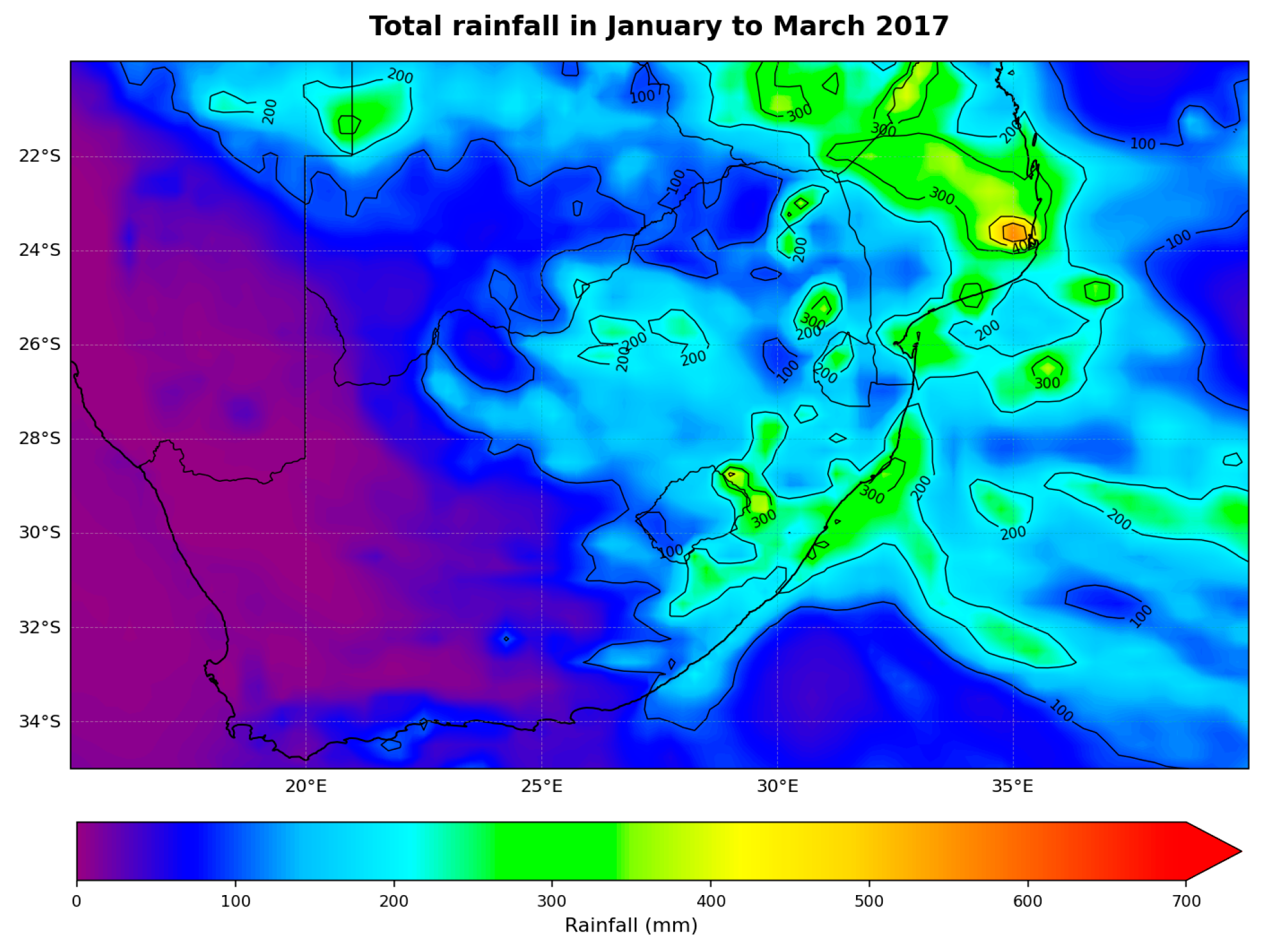
The Outgoing longwave radiation (OLR) was simulated for the months of January, February, and March (JFM) in the year 2017 across the designated study area. In the northern segment of the KwaZulu-Natal province (Figure 14), negative OLR values were observed during this timeframe. Areas identified as being more severely affected by extreme flooding are characterized by low OLR values (Figure 14). Botswana exhibited predominantly low OLR values, indicating that it was among the regions most affected by extreme heavy rainfall. The correlation between low OLR values and regions experiencing heavy rainfall highlights the utility of OLR as an effective indicator in identifying areas prone to extreme weather events in this study (Figure 14). South Africa, along with neighbouring countries such as Mozambique, Botswana, and Zimbabwe, experienced significant flooding during JFM 2017 (Figure 15).

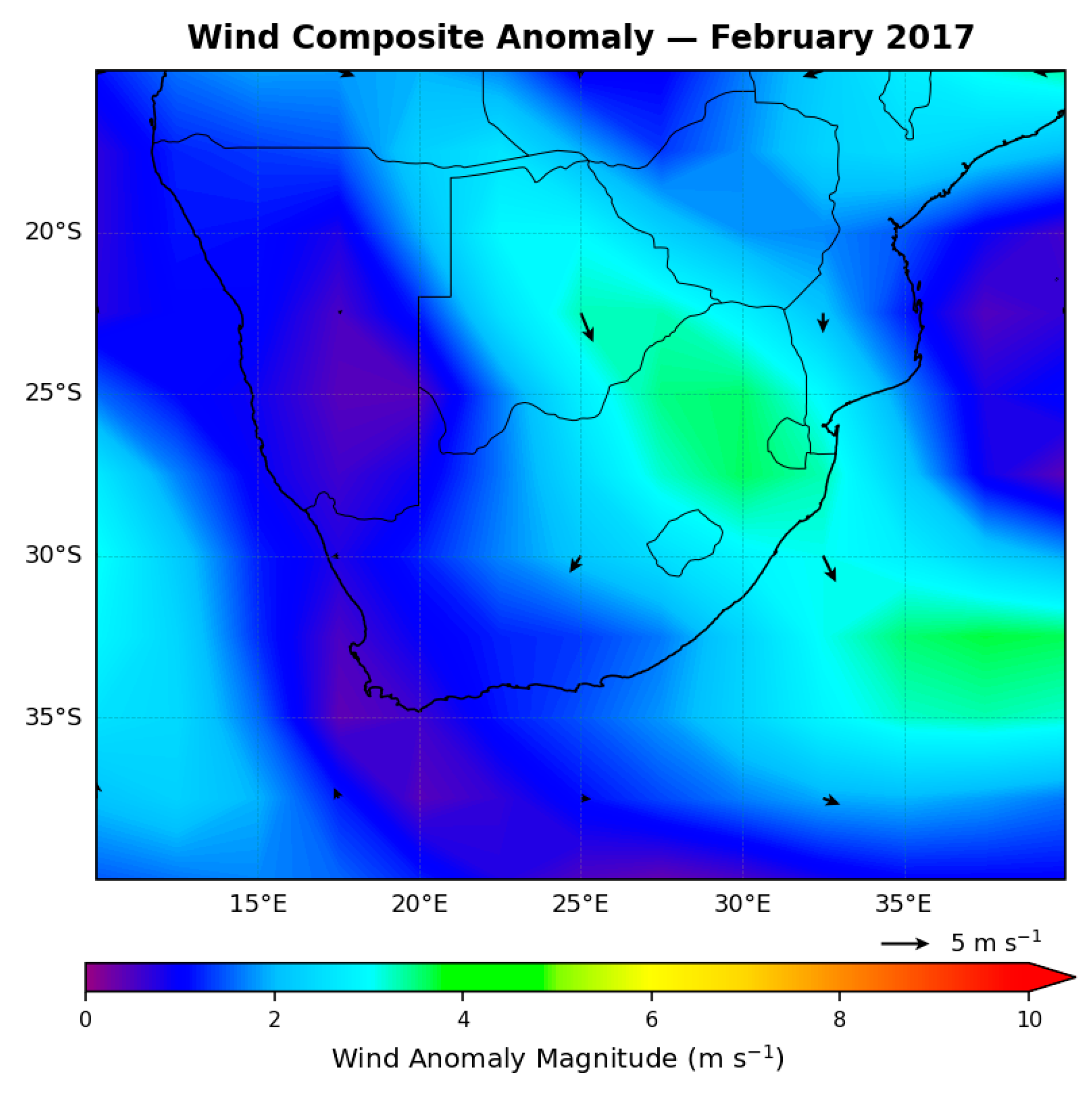
The wind anomalies modelled for February 2017 across the study region are shown in Figure 16. The north-easterly wind vector anomaly significantly contributes to the moisture transport, which sometimes causes extreme rainfall in southern Africa. These wind anomalies are an important element in causing summer flooding in the study area, occurring at both the surface level and the 500 hPa altitude (Figure 16). These anomalies signify deviations from the normal wind patterns and often indicate shifts in atmospheric circulation linked to large-scale weather phenomena. Wind vector anomalies are frequently linked with large-scale climate drivers, particularly latitudinal shifts in the Intertropical Convergence Zone (ITCZ), which enhance the transport of warm, moisture-laden air from the tropical Indian Ocean into southern Africa [32]. These anomalous circulation patterns strengthen low-level moisture convergence and uplift, creating favourable conditions for deep convection, widespread cloud development, and heavy rainfall over the region. These interactions highlight the significance of wind vector anomalies in comprehending the processes behind severe weather and flooding events in the region.

3.3.2. Tropical-Temperate Trough (TTT)

During the austral summer, another principal rainfall-generating mechanism over southern Africa consists of synoptic-scale tropical-temperate troughs (TTTs) [35]. This tropical-temperate trough system generates a cloud band accompanied by atmospheric convection that stretches in a northwest–southeast orientation, enveloping both the terrestrial area and the adjacent SWIO region [3]. Warmer SSTs over the southwest Indian Ocean can enhance moisture availability and transport towards southern Africa, particularly when accompanied by favourable easterly wind anomalies. These conditions increase moisture convergence over the region and can support the development of tropical-temperate troughs, which are important rainfall-producing systems during the austral summer [11].

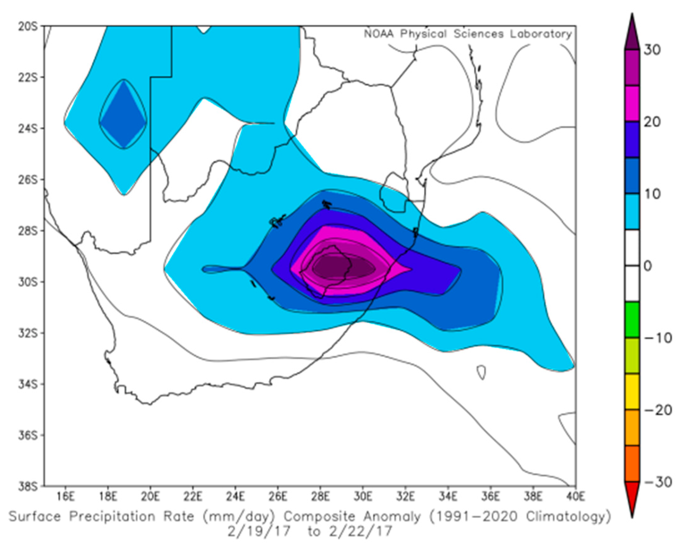
On 19 February 2017, the remnants of Cyclone Dineo were gradually dissipating over the extreme northwestern region of Namibia and were no longer associated with significant cloud formation or intense precipitation. Nonetheless, Dineo exerted a more substantial, though indirect, influence on atmospheric conditions from 19 to 22 February 2017. SAWS also issued a weather warning post on Tropical Cyclone Dineo regarding the expected rainfall over the country. In this case, we have further analyzed the extreme rainfall after 22 February 2017 over the KwaZulu Natal although the focus was on the progression of Tropical Cyclone Dineo.

Table 4. The weather station recorded >100 mm of rainfall from 19 to 22 February 2017. Source: SAWS.

Station Name	Coordinates	Rainfall (mm)
King Shaka Airport	−29.6108 31.1239	119.9
Margate	−28.9474 31.7079	109.4
Paddock	−30.7544 30.2577	110.2
Vanreenen	−28.3789 29.3885	173.0
Mtunzini	−28.9474 31.7079	161.0
Royal National Park	−28.6858 32.0934	183.2
Richards Bay Airport	−28.7378 32.0934	184.2

shows the recorded rainfall exceeding 100 mm from 19 to 22 February 2017 over KwaZulu-Natal.

The analysis indicates that the period following Tropical Cyclone Dineo provided favourable conditions for the development of a tropical-temperate-trough over southern Africa. The interaction between residual tropical moisture and mid-latitude circulation systems likely contributed to the formation of a northwest–southeast oriented cloud band typical of TTTs. This highlights the role of tropical-extratropical coupling in sustaining rainfall beyond the dissipation of tropical systems. The impacts are often more severe when TTTs occur together with other systems such as cut-off lows. For example, during the extreme rainfall event of 16–22 April 2006 over the southern Namib Desert, a cut-off low positioned unusually far north interacted with a TTT located further west than normal [35].

While tropical cyclones can produce intense, short-lived rainfall and widespread flooding over KwaZulu-Natal, their influence does not always end at landfall or dissipation. In several cases, including the post-Dineo period, the remnant circulation and associated moisture plumes interact with mid-latitude systems, creating favourable conditions for the development of tropical-temperate troughs (TTTs). These hybrid systems represent a critical linkage between tropical and extratropical dynamics, often sustaining or even enhancing rainfall over the subcontinent after the weakening of the parent cyclone. Consequently, understanding the transition from tropical cyclone activity to TTT formation is essential for explaining prolonged extreme rainfall episodes over southern Africa.

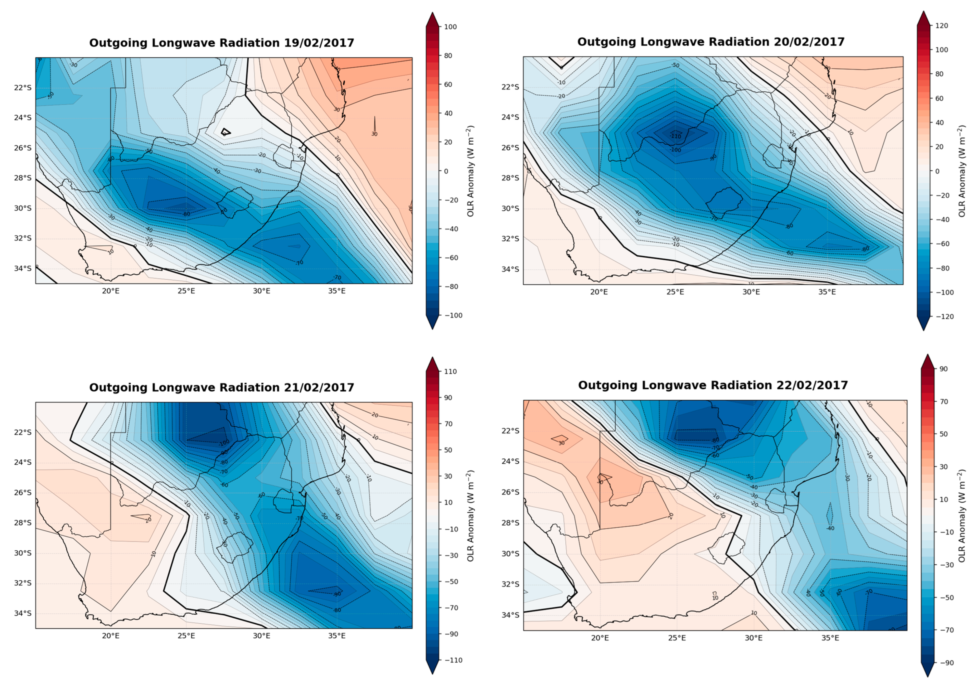
TTT systems originate from the interaction of two distinct meteorological components, both arising from different latitudinal regions [35]. The initial essential component is an upper atmospheric trough, which originates from the temperate mid-latitudes. In Southern Africa, this trough generally traverses the continent, commencing from the southern Atlantic Ocean and advancing eastward. The interaction of tropical and temperate air masses in proximity is a rare event. However, when it does occur, the combined system often has a strong potential to produce significant rainfall. The intense precipitation linked to significant TTT occurrences frequently leads to flooding throughout southern Africa. To better understand the mechanism behind TTT formation, a comprehensive analysis of the daily OLR was performed from 19 to 22 February, with the aim of identifying the cloud bands that are characteristic of these systems.

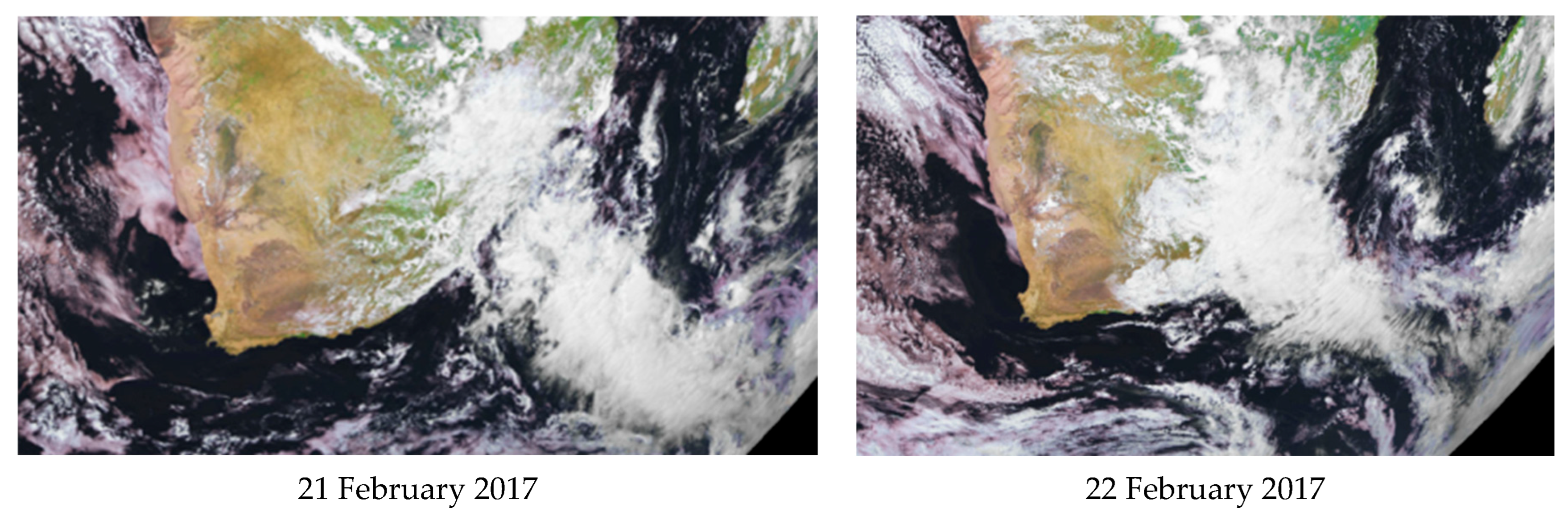
As depicted in Figure 16, negative OLR dominated over KwaZulu-Natal, South Africa, from 19 to 22 February 2017, and covered the Southeast Indian Ocean. TTTs serve as a crucial mechanism for transporting energy (heat), moisture, and momentum toward the poles; they are characterized by an area of increased convergence, typically recognizable by cloud bands [3,32,35]. Despite the incomplete understanding of the physical and dynamic characteristics of these systems at the synoptic scale [2,3,32,35], substantial research has been conducted to elucidate these crucial rain-generating systems, particularly in reference to this case study. The synoptic data from reanalysis, as depicted in Figure 14, show the ridge-trough-ridge configurations spanning both over the South African landmass and the Southeastern Indian Ocean. When TTT develops over a land area, the heating of the continent can support intense storms and heavy rain, unlike when TTT forms over the sea. This is supported by the rainfall analysis in Figure 15, which shows that daily rainfall over South Africa exceeded 20 mm per day from 19 to 22 February 2017. The SAWS surface station data recorded over 100 mm of rainfall at various stations in KwaZulu-Natal, as shown in Table 4.

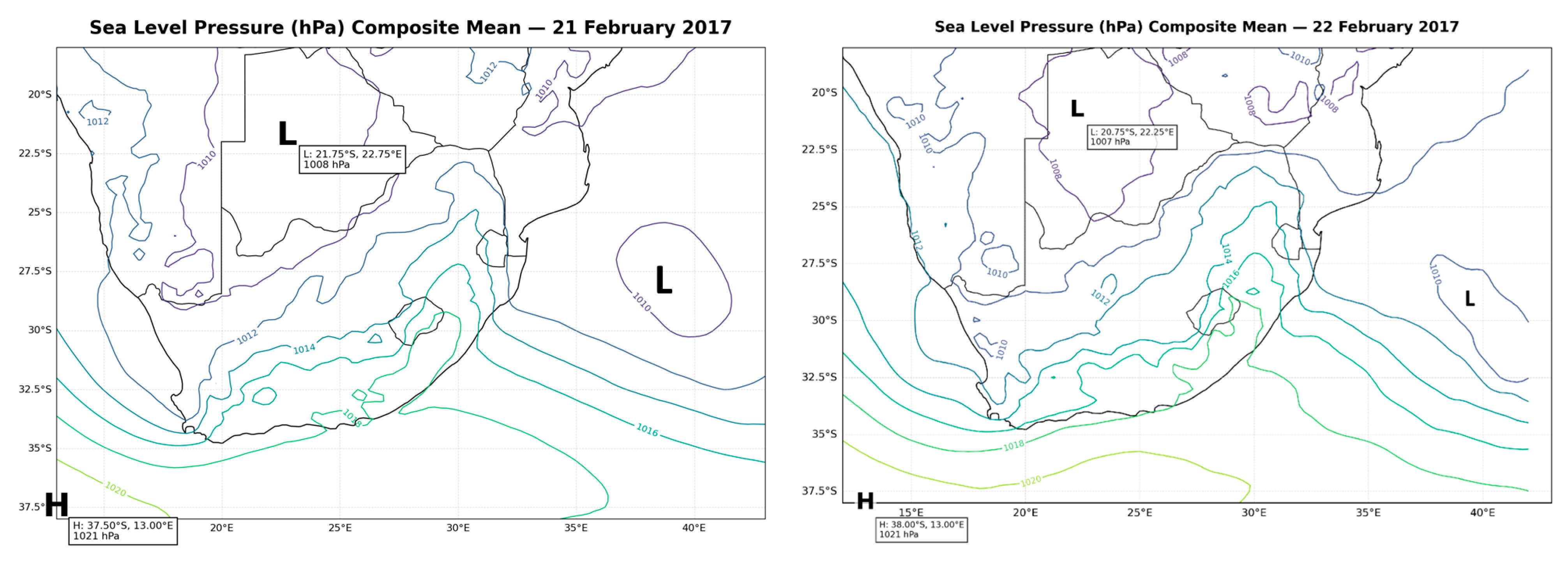
Numerous studies emphasize the correlation between the variability of annual rainfall in southern Africa and the occurrence, positioning, and strength of meteorological events such as TTTs [3]. For instance, during the wet spell from 1 to 7 January 1998, two successive TTTs contributed to over 40% of South Africa’s summer rainfall for that specific season [3]. A positive OLR anomaly over the SWIO is observed during a TTT event (Figure 17), which is normally caused by suppressed convective activity. The observed positive OLR over the SWIO indicates that there is less cloud cover and reduced deep convection over the area. The anomalous cloud band extends from the southeast Indian Ocean to northwest South Africa (Figure 17). It is evident that an area of increased convection is observed over the study region. As shown in Figure 18, the development of the cloud band aligns with sea-level pressure anomalies. Convection is also reduced over the southwest Indian Ocean, with the associated ridge extending from the northwest over KwaZulu-Natal to the southeast Indian Ocean (Figure 18). An anomalous cloud band, showing intensified convective activity, is observed over South Africa (Figure 18 and Figure 19). The characteristics and atmospheric structure of the TTT cloud band align with findings from prior research [9,18,36]. Following the dissipation of Cyclone Dineo, a TTT developed between 19 and 22 February 2017, producing additional rainfall exceeding 100 mm at selected stations. Composite OLR anomalies during this period reveal a northwest–southeast oriented cloud band extending from the tropical interior to the southwest Indian Ocean, characteristic of mature TTT systems. The results confirm that TTTs can prolong and intensify rainfall episodes initiated by tropical disturbances, demonstrating the importance of tropical-extratropical coupling mechanisms. The sea level pressure composite mean shows a persistent low-pressure centre over the northern interior of southern Africa, with the low located near 21.75° S, 22.75° E on 21 February and shifting to approximately 20.75° S, 22.25° E on 22 February 2017 (Figure 20). A broad high-pressure system of about 1021 hPa remains positioned to the southwest, while pressure gradients across southeastern southern Africa indicate the influence of contrasting pressure systems during the period (Figure 20). Overall, the pressure pattern suggests a continued low-pressure circulation over the region, with a slight westward/ northward displacement of the low centre between 21 and 22 February, consistent with changing atmospheric conditions during the cyclone period.

3.3.3. Cut-Off Lows

Cut-off Low (COL) systems were objectively identified independently of rainfall using their characteristic atmospheric circulation and thermal structure. A COL was identified based on the presence of a closed geopotential-height contour at 500 hPa, a cold-core structure at 200 hPa, separation from the main mid-latitude westerly flow, and persistence for at least 24 h. These criteria were applied to the 1990–2020 reanalysis record to identify the complete population of COL systems affecting the study area. Rainfall was not used as a criterion for the initial identification of COL events. Following the identification of the COL population, each event was temporally matched with daily rainfall observations from the SAWS stations. The seasonal distribution shows that COL events were most frequent during JJA (11 events), followed by SON (8), DJF (4), and MAM (1) (

Table 5. Seasonal distribution of identified COL events and their associated rainfall response during 1990–2020.

Seasons	COLs	≥50 mm	<50 mm
DJF	4	3	1
MAM	1	1	0
JJA	11	10	1
SON	8	6	2
Totals	24	20	4

). The maximum 24 h rainfall associated with each COL was then determined and used to classify the rainfall response. COL events associated with rainfall ≥ 50 mm day⁻¹ at one or more stations were classified as COL-associated extreme-rainfall events, while events with maximum rainfall below 50 mm day⁻¹ were retained as non-extreme-rainfall COL events (

Table 6. Identified COL events and associated maximum 24 h rainfall over KwaZulu-Natal during 1990–2020.

COL-ID	Dates	Seasons	Maximum Rainfall (mm)	Rainfall Class
COL-01	22–23 September 1993	SON	144.2	≥50 mm
COL-02	16–17 June 1995	JJA	43	<50 mm
COL-03	22–23 December 1995	DJF	60.2	≥50 mm
COL-04	07–09 July 1996	JJA	167.4	≥50 mm
COL-05	11–12 June 1997	JJA	177.6	≥50 mm
COL-06	25–26 October 1999	SON	75.2	≥50 mm
COL-07	15–16 January 2000	DJF	194.6	≥50 mm
COL-08	17-November 2000	SON	127.2	≥50 mm
COL-09	30 August 2001	JJA	50.6	≥50 mm
COL-10	18–20 Jul 2002	JJA	129.4	≥50 mm
COL-11	27 July 2004	JJA	108.4	≥50 mm
COL-12	26 September 2006	SON	153.8	≥50 mm
COL-13	17–18 June 2008	JJA	380	≥50 mm
COL-14	12 November 08	SON	114.6	≥50 mm
COL-15	09–10 June 2011	JJA	84.8	≥50 mm
COL-16	24–26 July 2011	JJA	110.6	≥50 mm
COL-17	7 August 12	JJA	147.4	≥50 mm
COL-18	10 December 2013	DJF	101.8	≥50 mm
COL-19	28–30 September 2014	SON	48	<50 mm
COL-20	24–25 July 2016	JJA	266.6	≥50 mm
COL-21	11–12 October 2017	SON	146.2	≥50 mm
COL-22	22–23 April 2019	MAM	234.6	≥50 mm
COL-23	22 January 2020	DJF	46.8	<50 mm
COL-24	2 October 2020	SON	20.4	<50 mm

). Thus, the 50 mm day⁻¹ threshold was used to classify the rainfall response of the identified COL rather than to define the COL population. For each COL event, the date, duration, season, maximum 24 h rainfall, rainfall-producing station, and rainfall classification were recorded (Table 6). Consecutive rainfall days associated with the same synoptic system were treated as a single COL episode when the atmospheric circulation satisfied the COL criteria throughout the event. COLs can generate 24 h rainfall amounts that surpass the usual monthly rainfall totals [37]. Seasonal projections across South Africa have predominantly concentrated on the summer precipitation zones during October to March (e.g., [38]), utilizing ENSO as the principal forecasting variable. It has been observed that there has been a shift in the preferred season for COL events from March–April–May (MAM) to June–July–August (JJA), and a shift in location from the southwest towards the northeast of subtropical southern Africa since the 1980s [1,39]. Cut-off lows (COLs) are cold-cored, synoptic-scale low-pressure systems in the middle and upper troposphere that develop through the detachment of an upper-level trough from the westerly flow. Over South Africa, COLs are commonly identified using closed circulations or geopotential-height minima at the 500 hPa level.

3.3.4. Frequency, Duration and Seasonal Variability of Cut-Off Lows (COLs)

A total of 24 COL events were identified during 1990–2020 using the atmospheric circulation and thermal criteria described in Section 3.3.3 (Table 6). The events occurred across all four austral seasons, with JJA recording the highest frequency (45.8%), followed by SON (33.3%), DJF (16.7%), and MAM (4.2%) (Table 6). The seasonal frequencies represent the occurrence of the identified COL population and were determined independently of rainfall magnitude. The rainfall response was subsequently evaluated for each identified COL. Of the 24 COL events, 20 (83.3%) were associated with maximum 24 h rainfall ≥ 50 mm at one or more SAWS stations, whereas four (16.7%) remained below the 50 mm day⁻¹ threshold. The latter events were retained in the analysis to provide a comparison population between COL occurrence and extreme-rainfall response. The seasonal distribution of COL-associated extreme rainfall was examined separately from the seasonal occurrence of all COLs. This distinction shows that the occurrence of a COL does not necessarily result in extreme rainfall and that the rainfall response depends on additional atmospheric conditions, including moisture availability, vertical motion, circulation persistence, and low-level moisture transport. The highest-rainfall COL events were subsequently selected for detailed case-study analysis to investigate the atmospheric mechanisms associated with particularly intense rainfall responses. The climatological analyses of COLs by [29,40], spanning the periods 1973 to 1982 and 1973 to 2002 respectively, identified a mean annual occurrence of 11 COLs, with the highest frequency recorded during the austral autumn March–April–May (MAM) season.

Consecutive rainfall days associated with the same COL circulation were treated as a single COL episode, and the maximum 24 h rainfall during each episode was used to classify the rainfall response. The threshold of 50 mm/24 h was applied after COL identification and was not used as a criterion for defining the COL itself. Full set of COL is also provided on (Table S1).

4. Case Study Cut-Off Low

Cut-off low events associated with the highest 24 h rainfall for each season were included in the study. The classification of COL systems was based on their circulation patterns, focusing on those events connected to unusual weather conditions and extreme rainfall. The following events were analyzed: 15–16 January 2000, 26 September 2006, and 22–23 April 2019. Each of these events recorded more than 50 mm of rainfall within 24 h and resulted in widespread precipitation. The analysis also considered daily rainfall data from nearby stations, with correlations assessed in relation to their elevation.

4.1. Cut-Off Low on 15–16 January 2000

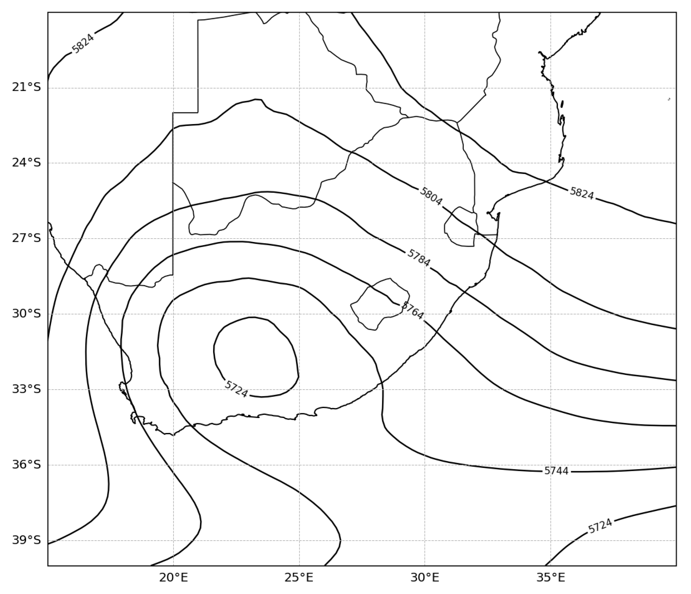
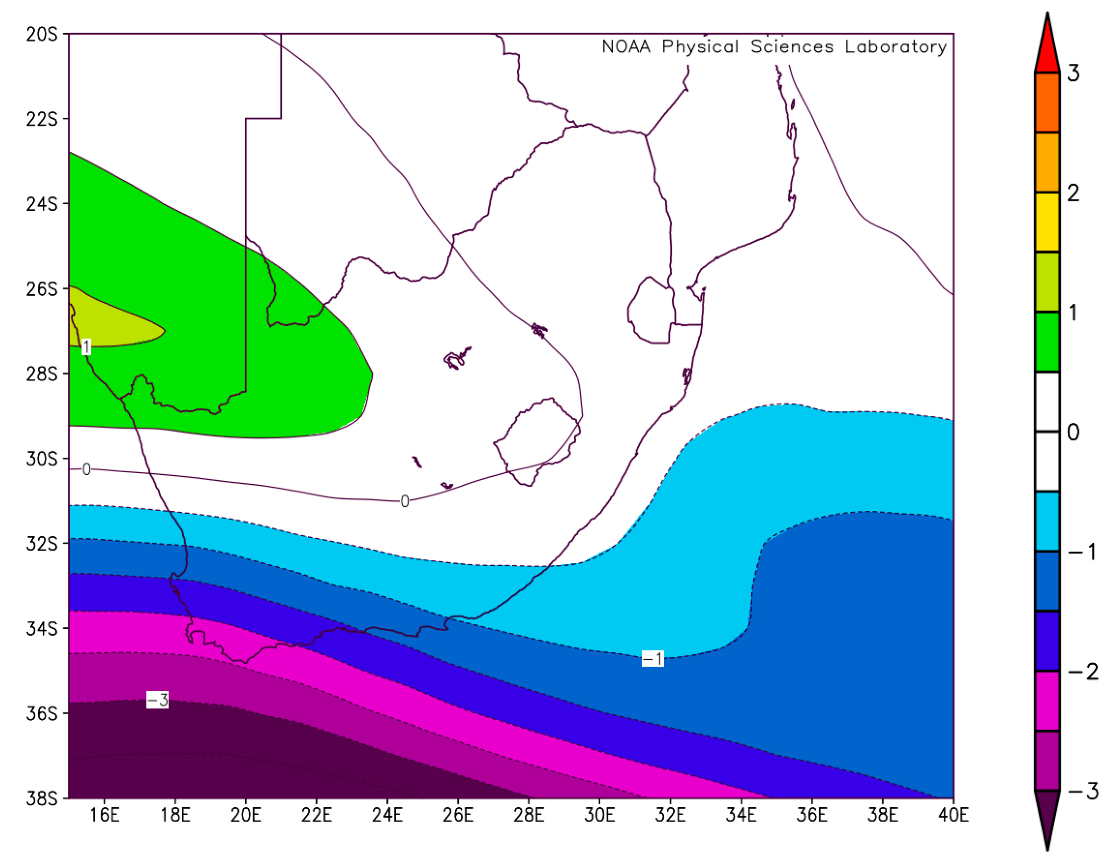
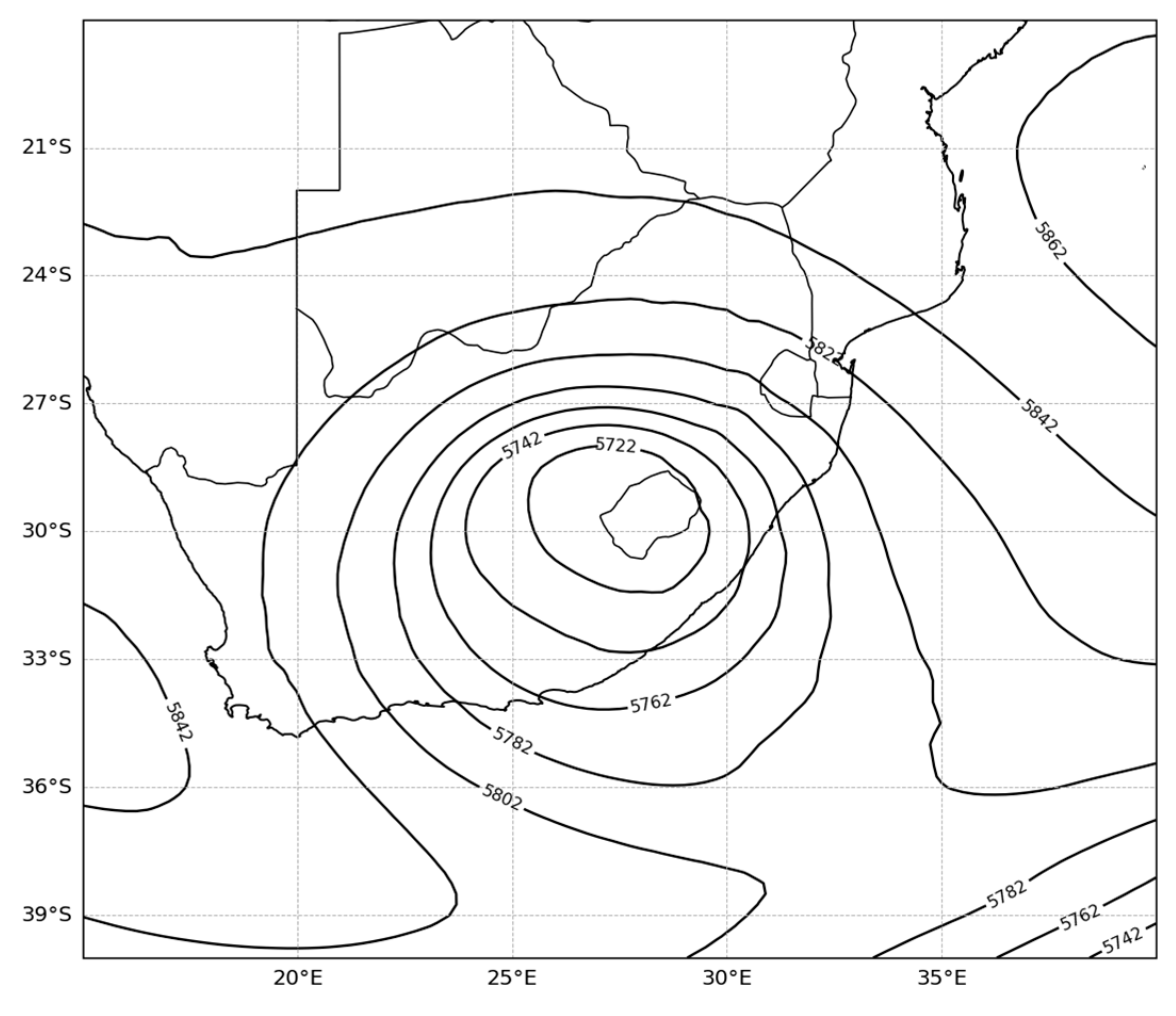
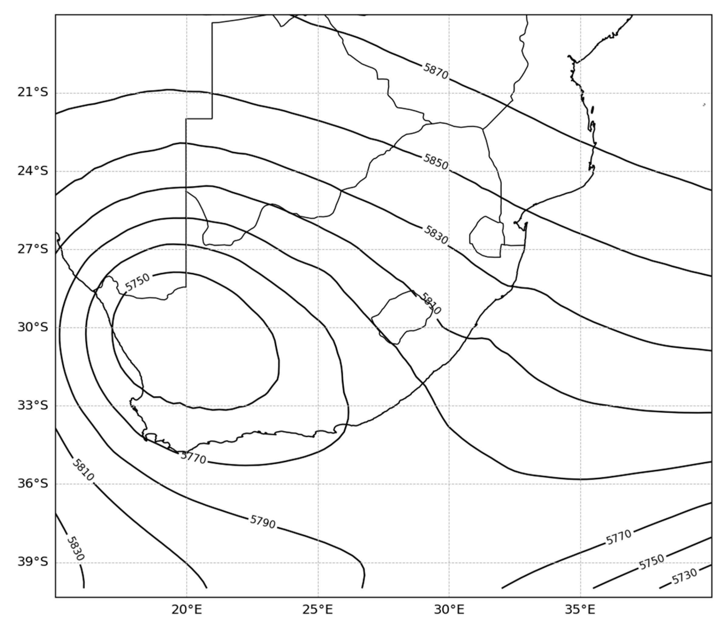
On 15 January, 64.2 mm of rainfall was recorded, followed by a significantly higher total of 194.6 mm on 16 January at the same station, both exceeding the 50 mm threshold within 24 h. As depicted in Figure 21, 500 hPa geopotential height fields during 15 January 2000 show a defined cut-off low-pressure system centered over southern Africa. This altitude, which is approximately equivalent to the middle of the troposphere (around 5.5 km above sea level), serves as an essential layer for analysing large-scale weather patterns such as COLs. Ref. [41] states that cut-off lows that persist for just one or two days are considered brief systems and are usually fast-moving and not very strong but associated with extreme rainfall over a short period. On 15 January 2000, the core of the weather system was sitting over the Western Cape and Eastern Cape provinces (Figure 21). On 15–16 January 2000, anomalously low sea level pressures were observed over southern Africa associated with a cut-off low (COL) system (Figure 22).

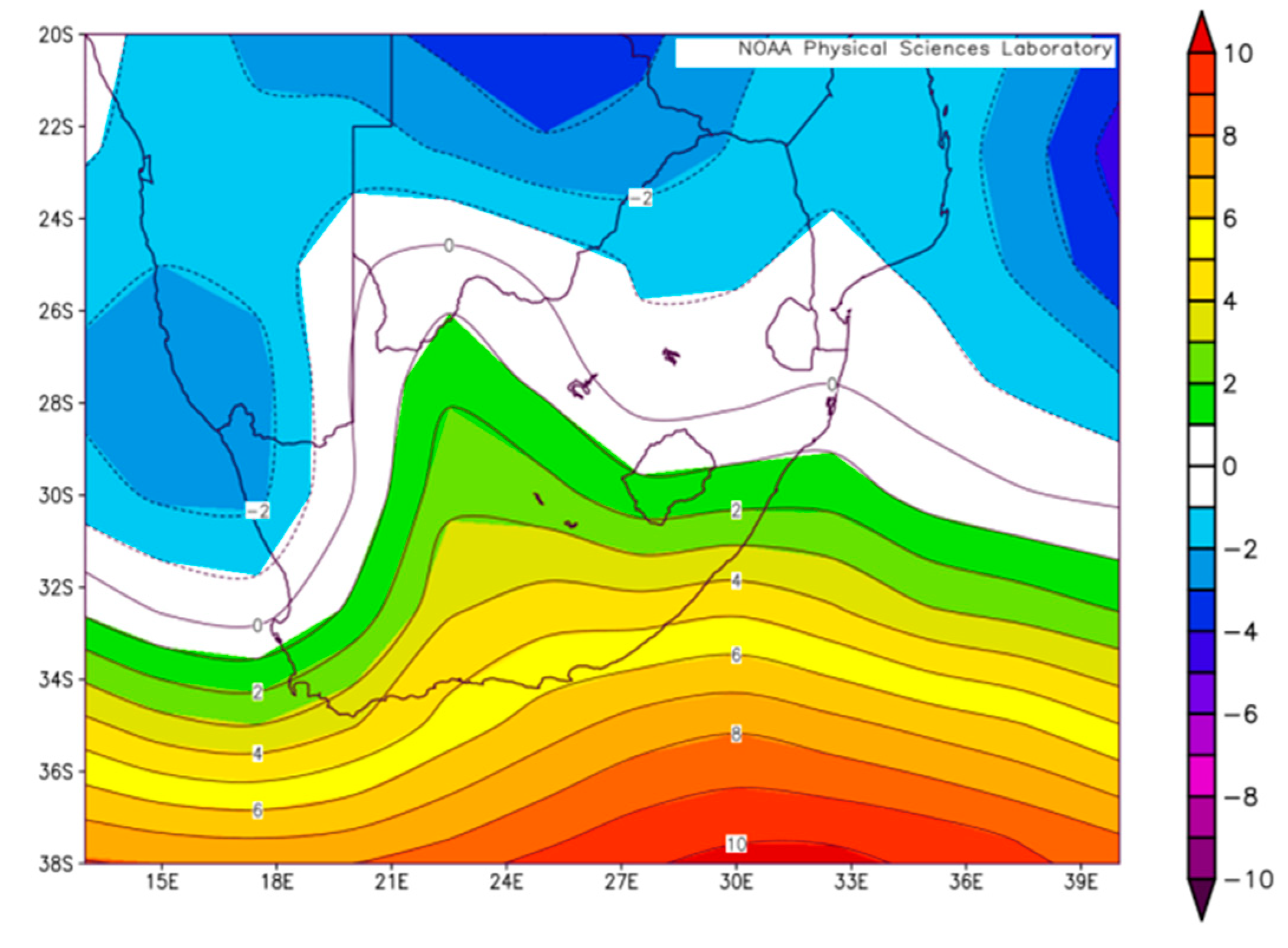
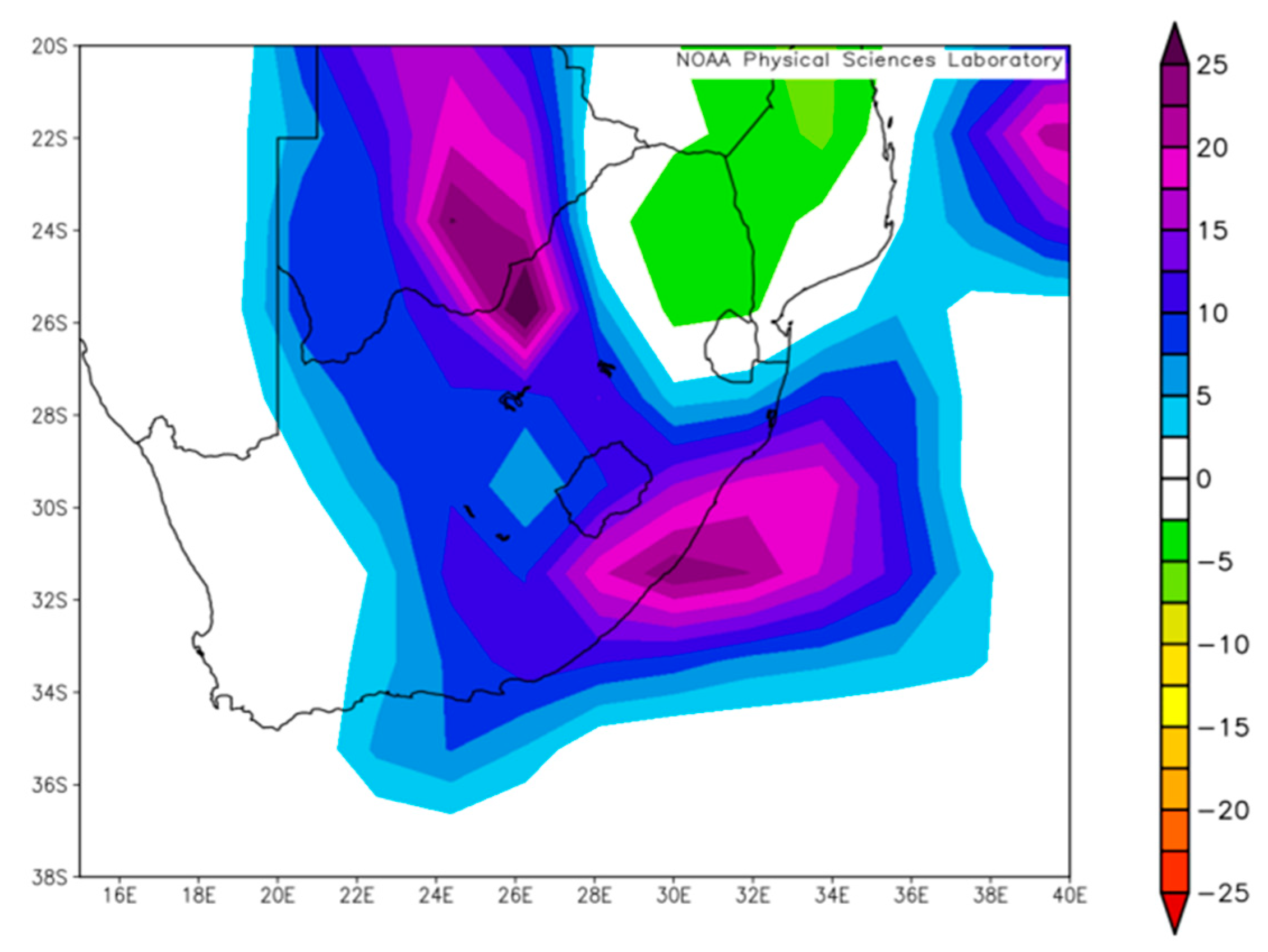
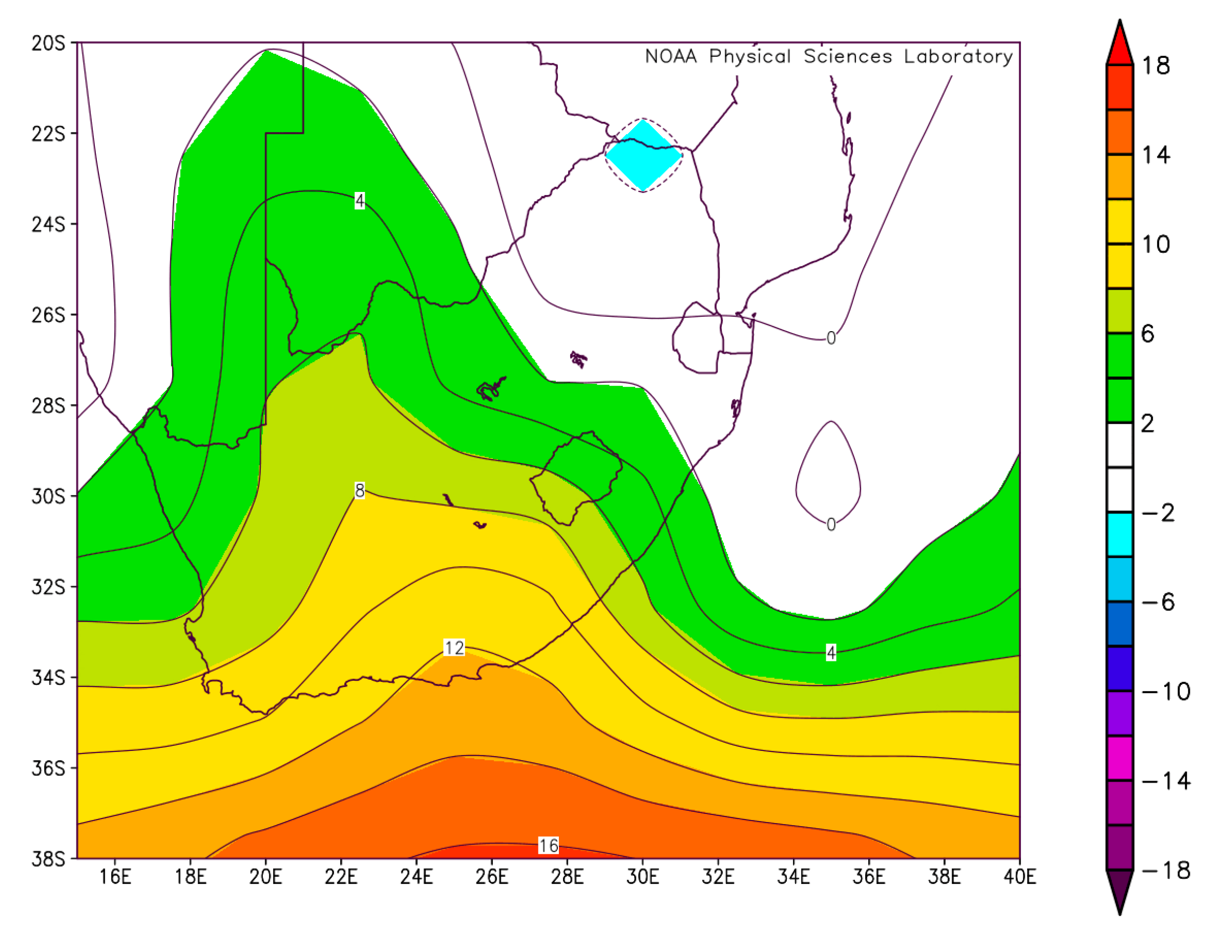
This upper-level disturbance, isolated from the main mid-latitude westerlies, became stationary over the region, creating favourable conditions for prolonged moisture convergence and vertical uplift. As a result, the COL system triggered widespread and intense rainfall, contributing to extreme flooding during this period. The air temperature at 200 hPa as shown on Figure 23, at this level, the COL was characterized by a cold core structure, and temperatures were significantly lower than the surrounding atmosphere. Temperature ranged from −1.2 °C to 1.2 °C. The system brought cold conditions over the southeastern Atlantic Ocean and the eastern part of the Indian Ocean, both characterized by negative anomalies (Figure 23), while the interior of the study area was dominated by positive temperature anomalies. This anomalous air temperature at 200 hPa is a characteristic structure of cut-off low-pressure systems [37]. Satellite-derived composite surface rainfall anomalies indicated accumulations ranging from 5 to 25 mm across these regions (Figure 24). The Paddock weather station within the study area recorded substantial daily rainfall totals of 64.2 mm on 15 January and 194.6 mm on 16 January 2000.

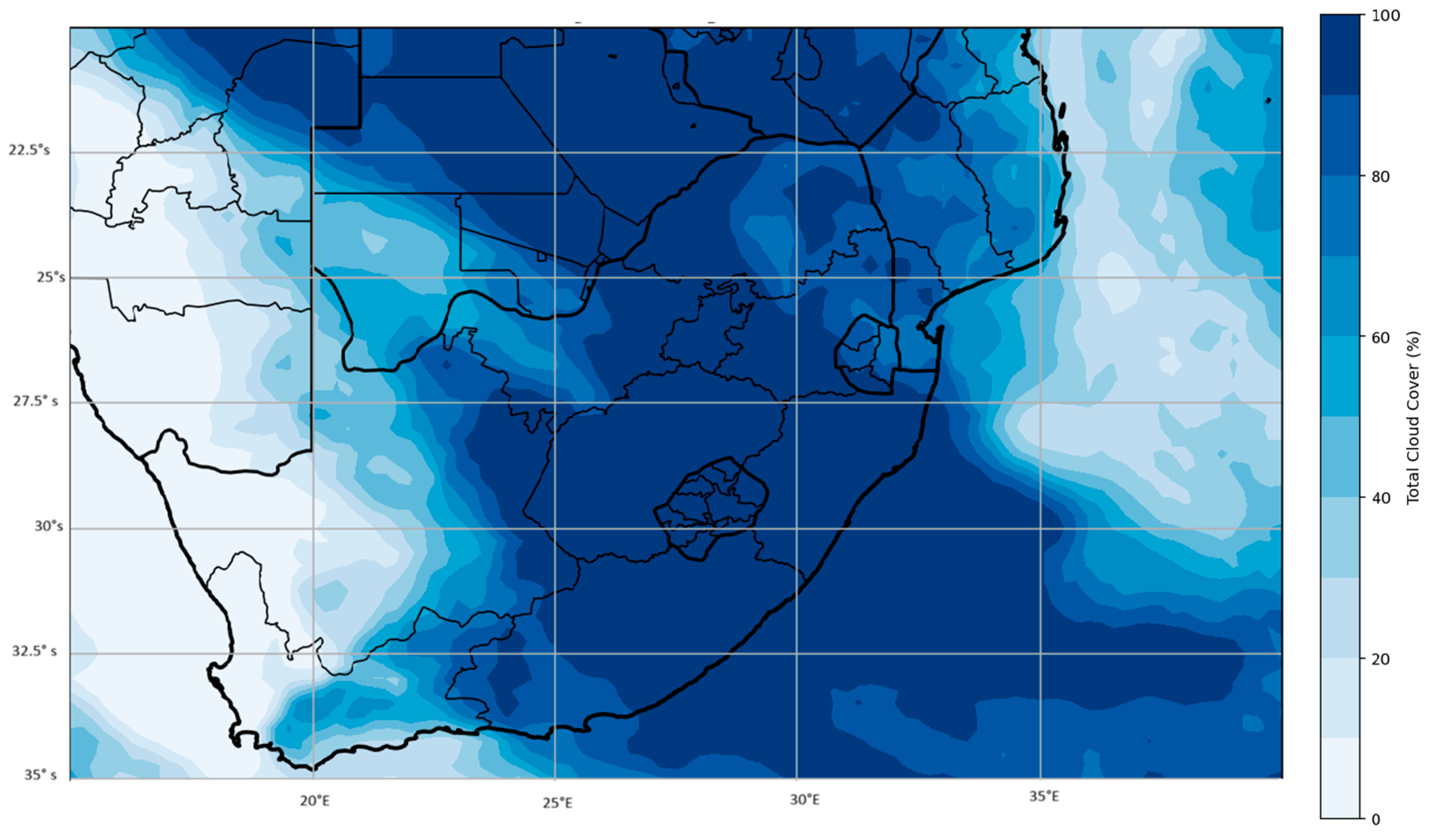
These observations closely aligned with rainfall estimates from the NCEP reanalysis dataset, confirming the accuracy of the satellite and model-based assessments (Figure 23). Area-averaged 500 hPa omega during 15–16 January 2000 reached approximately −0.20 to −0.25 Pa/s over the eastern escarpment region, indicating strong mid-tropospheric uplift relative to the 1990–2020 climatological mean. Concurrently, relative humidity at 500 hPa exceeded 80–85% across much of KwaZulu-Natal, creating a deeply saturated column favorable for sustained convection. The total cloud cover distribution on 15 January 2000 indicates extensive cloudiness (>80%) across much of South Africa, particularly over the central, eastern, and northeastern regions, reflecting widespread deep convective activity (Figure 25). These dynamical and thermodynamic conditions confirm that the extreme rainfall was associated with strong vertical motion combined with high mid-level moisture availability.

4.2. Cut-Off Low on 26 September 2006

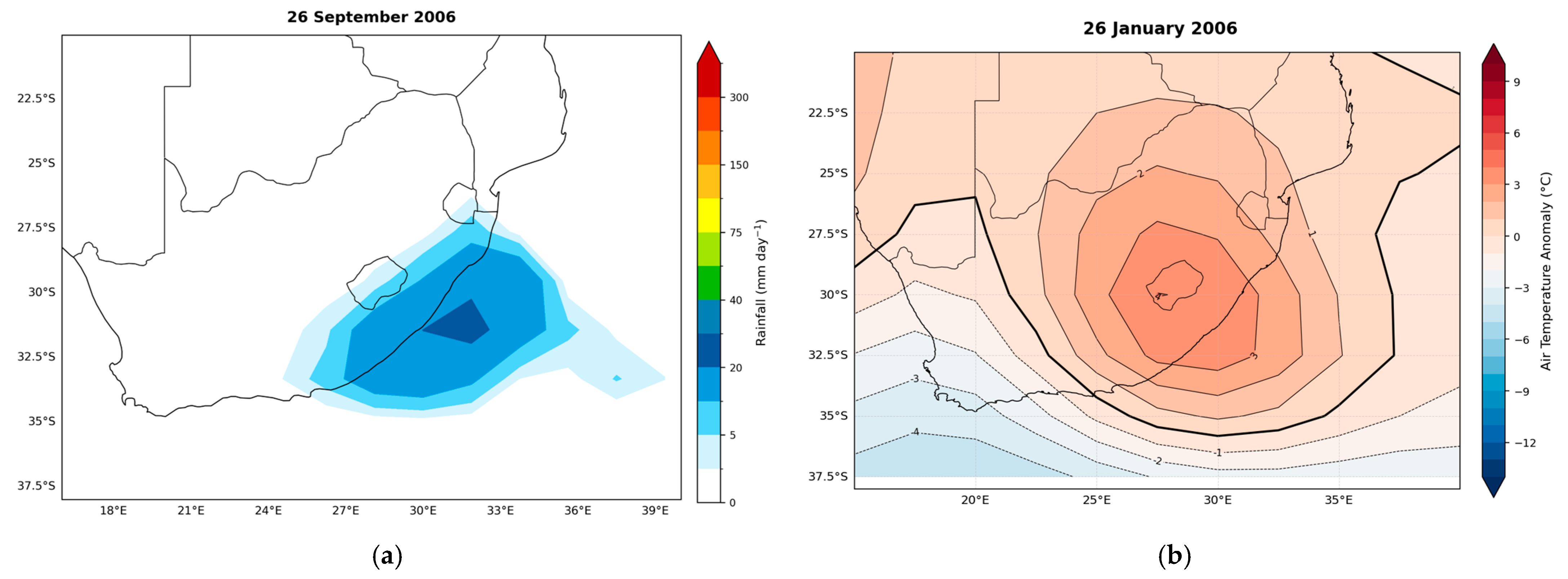
On 26 September 2006, South Africa experienced an extreme rainfall event associated with a cut-off low weather system. Rainfall exceeding 50 mm was recorded at several stations across multiple provinces, particularly in the Eastern Cape and KwaZulu-Natal. This significant meteorological event resulted in widespread heavy rainfall, leading to localized flooding, infrastructure damage, and disruptions to transport services. The area of study is notably impacted by this weather phenomenon, making it a key case for analyzing the effects and patterns of cut-off low systems in the region. In KwaZulu-Natal, one of the weather stations recorded 153.8 mm of rainfall within a 24 h period, and this data is used for analysis in this study. Although short-lived cut-off low systems are often not expected to cause significant societal impacts, this event produced extreme rainfall within a single day, highlighting the potential severity of even brief cut-off low occurrences. Despite its limited lifespan, the system generated rainfall levels typically associated with high-impact weather events. As shown in Figure 26, the 500 hPa geopotential height fields for 26 September 2006 clearly indicate a well-developed cut-off low pressure system positioned over the study area.

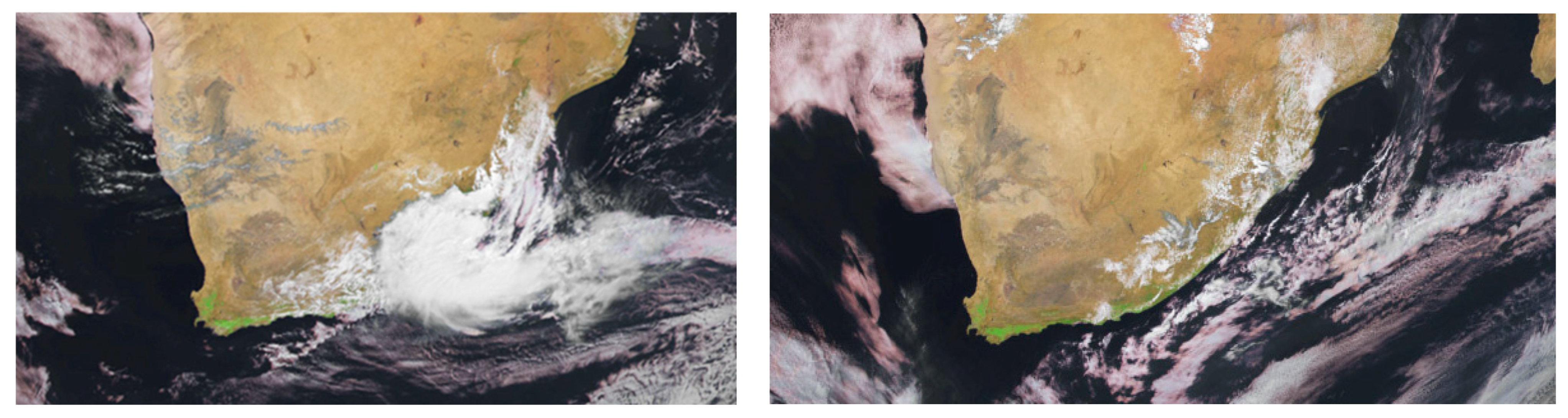
At the 200 hPa pressure level (Figure 27), the center of the COL is characterized by significantly colder air aloft. Over the Eastern Cape and KwaZulu-Natal regions, notably lower temperatures were observed in association with this upper-level system. As the COL was a transient system, valid for only a single day, it nonetheless contributed to notably cooler conditions across the study area. Satellite imagery (Figure 28) reveals dense convective cloud development, particularly cumulonimbus (Cb) clouds, which are typically associated with localized thunderstorms and heavy showers. On the following day, the system progressed eastward into the southwestern Indian Ocean, where it began to dissipate, accompanied by a reduction in rainfall intensity (Figure 29a).

Additionally, high-level cirrus clouds exhibiting hook-like formations were identified, indicating the presence of upper-level divergence and strong outflow often linked to dynamic convective systems. Anomalous rainfall from the NCEP reanalysis (Figure 29a) indicates precipitation anomalies over the Eastern Cape and KwaZulu-Natal, ranging from 5 mm to 21 mm. However, significantly higher totals were recorded by the South African Weather Service (SAWS), with KwaZulu-Natal stations such as Paddock recording 153.8 mm and Margate 102.0 mm over a 24 h period.

These coastal stations highlight the localized intensity of rainfall associated with the COL event. The center of the summer COL exhibited a slightly higher temperature (3 °C) than its surroundings, where temperatures in the Southeast Indian Ocean dropped from 2 °C to −2 °C, the air temperature at 200 hPa, as shown in Figure 29b. During peak rainfall on 26 September 2006, 500 hPa omega values over the eastern coastal belt were estimated at approximately −0.18 to −0.22 Pa/s, indicating significant upward vertical motion despite the system’s short lifespan. Relative humidity at mid-levels exceeded 85% over KwaZulu-Natal, confirming a moisture-rich environment conducive to deep convective development. The combination of strong localized uplift and high atmospheric moisture content explains the intense 24 h rainfall totals recorded at coastal stations.

4.3. Cut-Off Low 22–23 April 2019

The observed cut-off low (COL) system led to extreme rainfall and widespread flooding across parts of South Africa between 22 and 25 April 2019, coinciding with the Easter holiday weekend. During this period, the COL produced sustained and intense precipitation, with recorded rainfall totals ranging from 150 to 200 mm over a 48 h period [41]. The 500 hPa geopotential height field for 22–23 April 2019 shows a well-defined COL over the southwestern interior of South Africa, characterized by closed geopotential height contours centered (Figure 30). Flooding associated with this rainfall event resulted in the displacement of over 40,000 people, more than 500 deaths, and reports of dozens of missing people [42]. Vulnerable communities, townships, informal settlements, and even developed urban areas were severely affected.

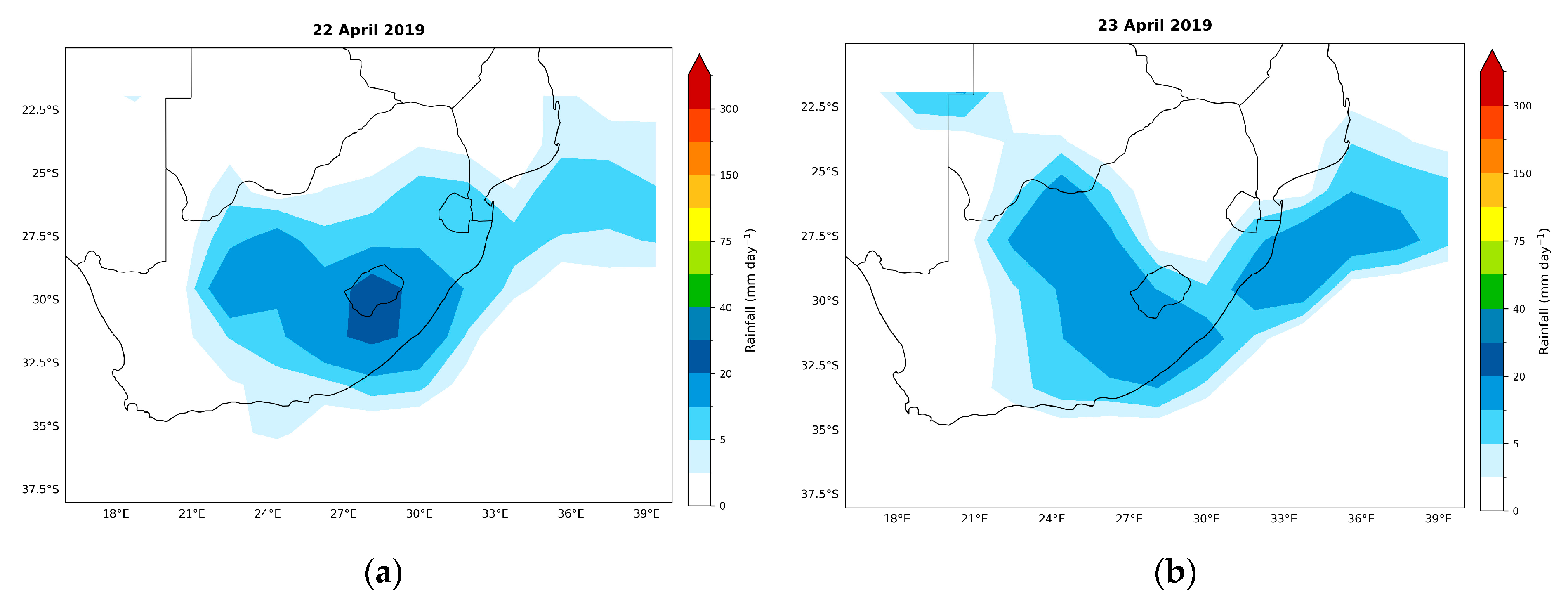
The anomalous rainfall reanalysis image on 22 April 2019 (Figure 31) shows above-average precipitation over the study area, where more than 25 mm was recorded. Daily analyses clearly depict this localized extreme event as moisture convergence, and the uplift resulted in an extreme rainfall event. The extreme and anomalous nature of this rainfall was clearly linked to this cut-off low. In KwaZulu-Natal, one of the stations recorded 234.6 mm of rainfall in 24 h, which correlates with NCEP daily reanalysis data for this case study (Figure 31). The interaction of warm moisture from the Indian Ocean plays a pivotal role, with strong uplift from the upper-level system triggering intense convective rainfall, especially over the eastern parts of South Africa (KwaZulu-Natal, Eastern Cape, Mpumalanga, and Gauteng). This system lasted for two days, causing floods over the study area, as shown in Figure 31a,b, from 22 to 23 April 2019, because the COLs are known as a slow-moving system. The complete station metadata are provided in Table S2.

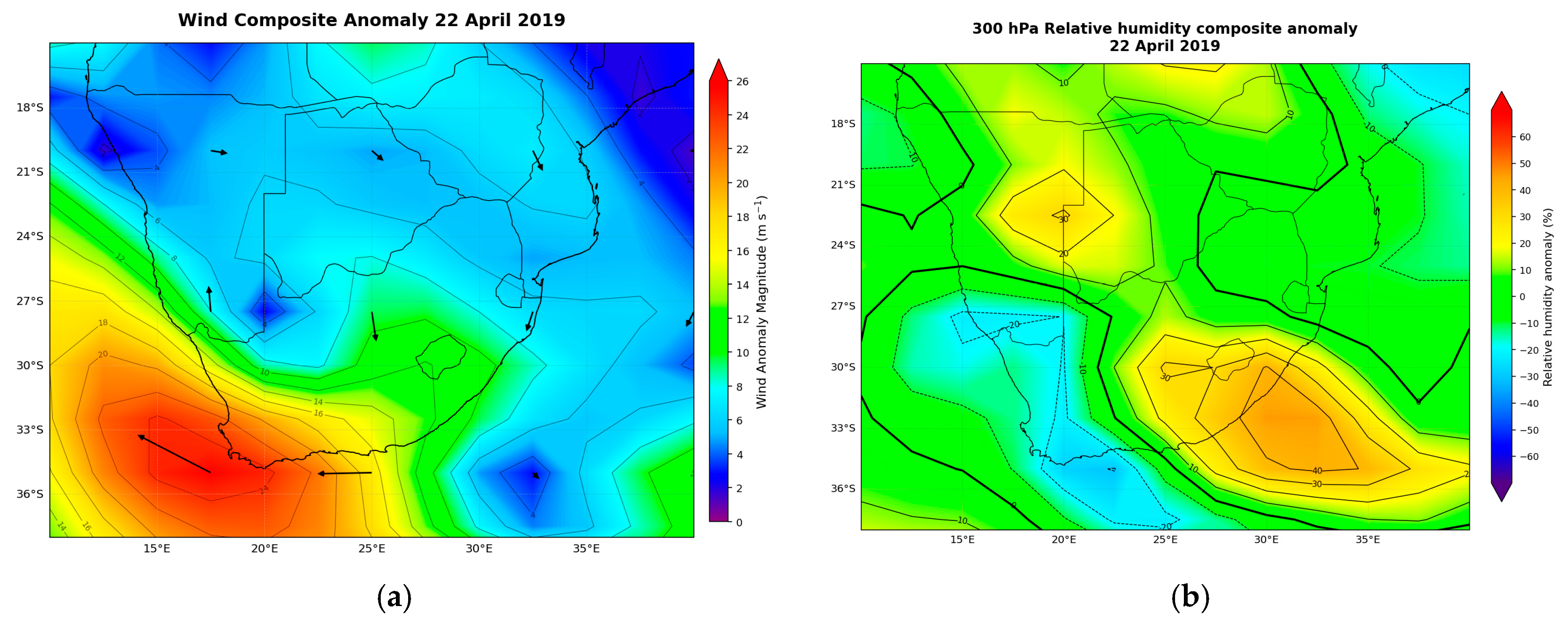
The analysis of 500 hPa wind anomalies from 22 to 23 April 2019 provides important insight into the dynamical processes driving the extreme rainfall event. Wind anomalies are calculated by subtracting the long-term climatological mean wind field for that period from the actual observed or reanalysed wind field on the day. At this level (500 hPa), it shows the steering currents for surface weather conditions and is used to identify vorticity advection. The major driver of extreme rainfall was not the COL in separation, but its interaction with moisture sources Figure 32 over South Africa. As depicted in Figure 32a, the circulation of the wind vector was dominated by northerly to southeasterly wind anomalies in the mainland and East of the Indian Ocean. These anomalous winds act as the large-scale advection of warm, moist, tropical boundary layer air masses from the Southwest Indian Ocean and the Mozambican Channel, resulting in a sustained, onshore moisture flux toward the eastern coastal regions of South Africa [1].

The wind vectors were observed in a north-easterly anomaly, channeling tropical moisture inland and sustaining large-scale uplift through cyclonic vorticity advection (Figure 32a). As the cut-off low covered the escarpment of the Eastern Cape and KwaZulu -Natal, moist north-easterly flow was forced to rise over the escarpment, enhancing rainfall through orographic lift. This is also supported by the study of extreme precipitation and flooding over South Africa, as the steep orography of the eastern escarpment acts as a trigger for deep convection and provides a persistent mechanism for amplifying rainfall under favorable atmospheric conditions [1]. At 500 hPa, Relative Humidity in middle levels was observed between 80 and 90% over the study area southeast of the Indian Ocean, extending to the mainland in Figure 31b from 22 to 23 April 2019. The northern and southern regions of the country experienced below-normal relative humidity conditions Figure 32b less than 30% HR. Wind vector anomalies indicated moisture transport primarily from the southwest Indian Ocean, with limited continental contribution from the western interior.

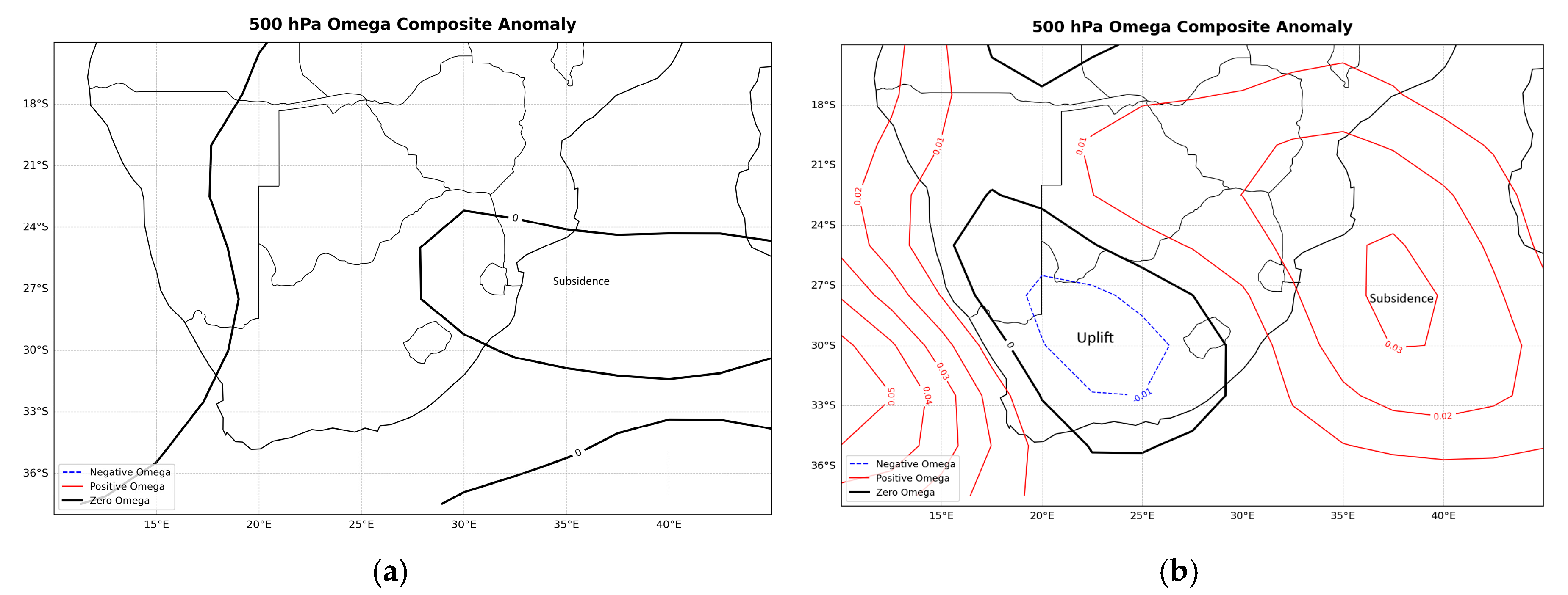
The composite analysis of the cut-off low system, observed Omega (Pa/s) composite anomaly during El Niño seasons from 1990 to 2020, shows that the interior experiences subsidence whilst the uplift region is over the southeastern Indian Ocean (Figure 32b). This shift means that the interior of South Africa lies under subsidence (sinking motion) rather than uplift. In the observed La Niña season, using composite analysis Omega at 500 hPa from 1990 to 2020, COLs tend to dominate over the southern interior and coastal areas over South Africa (Figure 33). In South Africa, La Niña seasons are commonly associated with above-average summer rainfall, as COLs driven by wetter, high-moisture circulation can generate widespread extreme rainfall events. Atmospheric warming is driven by the substantial scale of subsidence in the mainland. The surrounding high-pressure system is also linked with subsidence during a cut-off low, which also brings clear weather conditions, as precipitation does not normally occur in the middle of a high-pressure system. It is also considered in this study that cut-off lows and ENSO are not the same, as the cut-off low life span is 1–2 days or 1–3 days, and ENSO is a seasonal phenomenon. The large-scale subsidence over the interior contributed to atmospheric warming, as subsiding air warms adiabatically.

5. Discussion

The results support a multiscale interpretation of extreme rainfall over KwaZulu-Natal. The absence of statistically significant long-term trends in annual rainfall, combined with the strong seasonal ENSO relationship and the high proportion of identified COLs associated with extreme rainfall, indicates that rainfall risk is not adequately described by changes in seasonal totals alone. Large-scale climate variability, particularly ENSO during the summer season, influences the background moisture and circulation environment, while synoptic disturbances provide the immediate dynamical forcing for heavy rainfall. The COL analysis further demonstrates that even within a population of objectively identified systems, rainfall responses vary substantially, with 20 of 24 events exceeding 50 mm day⁻¹ and four producing lower rainfall. Tropical cyclones and TTTs provide additional pathways through which moisture transport, convergence, and uplift can produce high-impact rainfall. This interaction between background climate state, synoptic forcing, and regional topography provides a more physically consistent explanation for the spatial and temporal variability of extreme rainfall across KwaZulu-Natal. The spatial concentration of extreme rainfall along the eastern escarpment and coastal belt is consistent with studies showing enhanced convective development where onshore northeasterly flow interacts with steep topography [42]. By linking station observations with reanalysis diagnostics (OLR, geopotential height, omega, wind vectors, and relative humidity), this study extends previous work by explicitly demonstrating the dynamical and thermodynamic anomalies associated with these rainfall maxima. The agreement between observed station data and ERA5/NCEP reanalysis fields strengthens confidence in the identified mechanisms.

The ENSO analysis further demonstrates that large-scale climate variability primarily modulates the background rainfall environment rather than directly determining the occurrence of individual extreme events. The strongest and most consistent relationship occurred during DJF, when the regional rainfall index was negatively correlated with Niño 3.4 anomalies at zero- to three-month lags (r = −0.447 to −0.419; p = 0.013–0.021). This indicates that warmer Niño 3.4 conditions were associated with reduced summer rainfall across the regional station network. However, the absence of significant relationships during MAM, JJA, and SON indicates that the ENSO influence is seasonally dependent. The occurrence of high-impact rainfall events during neutral ENSO conditions further demonstrates that ENSO alone cannot explain event timing or intensity. Instead, ENSO appears to provide a large-scale modulation of the moisture and circulation environment within which synoptic systems such as COLs, TTTs, and tropical disturbances operate. This variability provides additional context for the present findings, where La Niña conditions enhanced large-scale moisture availability but did not solely determine the occurrence of extreme rainfall events. Instead, synoptic-scale disturbances governed event timing and intensity, reinforcing the need to integrate seasonal climate outlooks with sub-seasonal and synoptic diagnostics for operational forecasting.

However, the occurrence of several high-impact rainfall events during neutral ENSO conditions supports arguments that synoptic-scale disturbances are the direct rainfall-generating mechanisms, while ENSO modulates the background state [42]. Composite omega analyses further illustrate this multiscale interaction: La Niña enhances atmospheric moisture availability and large-scale uplift potential, while embedded systems such as cut-off lows (COLs), tropical cyclones (TCs), and tropical–temperate troughs (TTTs) act as immediate triggers.

The identification of 20 COL events producing ≥50 mm in 24 h, including the April 2019 event exceeding 200 mm, underscores the uneven contribution of short-duration systems to extreme rainfall totals. Previous studies have identified COLs as major contributors to heavy rainfall and flooding in eastern South Africa [3,29]. However, the seasonal peak identified here in JJA contrasts partially with earlier climatology emphasizing MAM dominance, suggesting possible decadal variability or circulation shifts. While differences in study period may partly explain this discrepancy, the results may also reflect broader circulation changes under a warming climate [43].

Tropical cyclones and TTTs were likewise shown to significantly contribute to extreme rainfall, particularly during late summer. The Dineo case study illustrates how weakening tropical systems can still generate substantial inland flooding when interacting with favourable pressure gradients and sustaining moisture flux convergence. Similarly, TTT-associated cloud bands produced prolonged rainfall exceeding 100 mm at several stations. These findings reinforce the importance of coupled tropical-extratropical dynamics in southern African hydroclimate variability [44,45]. Ref. [46] show that COLs occur throughout the year and can produce anomalously high rainfall, with some systems extending to the surface and producing conditions favourable for extreme rainfall and flooding, particularly where circulation interacts with the South African escarpment.

In the broader climate-risk context, the results highlight that extreme rainfall in KZN is driven more by changes in event intensity and synoptic frequency than by gradual increases in seasonal totals. This distinction aligns with global evidence that disaster losses are increasing due to both enhanced exposure and intensification of extreme events. Under continued atmospheric warming, increased moisture-holding capacity may amplify rainfall intensity even if circulation frequencies remain unchanged. While this study focuses primarily on atmospheric drivers of extreme rainfall, effective disaster risk reduction requires integration of hazard analysis with governance and vulnerability assessment frameworks. Disaster risk reduction in South Africa must adopt a multi-sphere approach, incorporating scientific hazard monitoring, institutional capacity, and community-level resilience. In the context of KwaZulu-Natal, where synoptic-scale disturbances frequently trigger high-impact flooding, the improved understanding of multiscale rainfall drivers presented here provides critical scientific input to support integrated flood risk governance and early warning system strengthening. Therefore, integrating ENSO outlooks with synoptic diagnostics could improve impact-based forecasting and early warning systems.

Future research should extend the analysis beyond 2020 to assess whether observed seasonal shifts in COL dominance persist. High-resolution regional climate modelling would help resolve mesoscale convective processes and orographic enhancement, particularly along the escarpment-coastal interface. Event attribution studies separating thermodynamic (moisture-driven) from dynamic (circulation-driven) contributions would clarify the relative influence of climate change. Finally, coupling meteorological diagnostics with hydrological impact models would improve understanding of how extreme rainfall translates into flood magnitude across heterogeneous catchments. Overall, the findings contribute to the growing body of evidence that multiscale atmospheric coupling governs extreme rainfall variability in eastern South Africa and provide a strengthened scientific basis for climate-informed disaster risk management in KwaZulu-Natal.

6. Conclusions

This study provides a comprehensive assessment of the spatiotemporal variability and multiscale drivers of extreme rainfall in KwaZulu-Natal over the 1990–2020 period. The findings suggest that extreme rainfall is mainly driven by short-duration, high-intensity events associated with synoptic-scale weather systems that develop under favourable large-scale moisture conditions. A key contribution of this study is the integrated evaluation of multiple atmospheric drivers, demonstrating that tropical-extratropical interactions play a dominant role in shaping extreme rainfall variability. Cut-off lows (COLs), tropical cyclones (TCs), and tropical-temperate troughs (TTTs) emerged as the primary synoptic-scale mechanisms triggering extreme rainfall events, highlighting the important role of these systems in modulating rainfall variability over the region. In contrast, large-scale modes such as ENSO primarily influence background moisture conditions rather than directly controlling event occurrence. The variability in the occurrence of cut-off low systems suggests possible shifts in atmospheric circulation patterns with implications for future climate conditions. These findings highlight the limitations of relying solely on seasonal-scale climate predictions for anticipating extreme rainfall events. Instead, improved forecasting requires integrating large-scale climate indicators with real-time synoptic analysis, particularly for rapidly evolving high-impact weather systems. This is especially important for KwaZulu-Natal, where flooding is frequently driven by short-lived but intense atmospheric disturbances. From an applied perspective, this study contributes to the advancement of impact-based forecasting and climate-informed disaster risk management by providing a clearer understanding of the processes driving extreme rainfall. Future research should extend the temporal scope, incorporate high-resolution modelling to better resolve mesoscale processes, and strengthen linkages between atmospheric drivers and hydrological responses to improve projections of flood risk under changing climate conditions. Overall, this study enhances understanding of the multiscale dynamics governing extreme rainfall in eastern South Africa and supports efforts to improve resilience to climate-related hazards.

References

1. Singleton, A.T.; Reason, C.J.C. Variability in the characteristics of cut-off low pressure systems over subtropical southern Africa. Int. J. Climatol. 2007, 27, 295–310. [Google Scholar] [CrossRef] [Scilit]
2. Nicholson, S.E. Climatic and environmental change in Africa during the last two centuries. Clim. Res. 2001, 17, 123–144. [Google Scholar] [CrossRef] [Scilit]
3. Hart, N.C.G.; Reason, C.J.C.; Fauchereau, N. Tropical–extratropical interactions over southern Africa: Three cases of heavy summer season rainfall. Mon. Weather Rev. 2010, 138, 2608–2623. [Google Scholar] [CrossRef] [Scilit]
4. Malherbe, J.; Engelbrecht, F.A.; Landman, W.A.; Engelbrecht, C.J. Tropical systems from the southwest Indian Ocean making landfall over the Limpopo River Basin, southern Africa: A historical perspective. Int. J. Climatol. 2012, 32, 1018–1032. [Google Scholar] [CrossRef] [Scilit]
5. Mann, H.B. Nonparametric tests against trend. Econometrica 1945, 13, 245–259. [Google Scholar] [CrossRef] [Scilit]
6. Erasmus, M. Formation and Development of Tropical Temperate Troughs Across Southern Africa as Simulated by a State-of-the-Art Coupled Model. Master’s Thesis, University of Pretoria, Pretoria, South Africa, 2019. Available online: https://hdl.handle.net/2263/73478 (accessed on 13 June 2025).
7. Fauchereau, N.; Trzaska, S.; Rouault, M.; Richard, Y. Rainfall variability and changes in southern Africa during the 20th century in the global warming context. Nat. Hazards 2003, 29, 139–154. [Google Scholar] [CrossRef] [Scilit]
8. Vigaud, N.; Pohl, B.; Crétat, J. Tropical–temperate interactions over southern Africa simulated by a regional climate model. Clim. Dyn. 2012, 39, 2895–2916. [Google Scholar] [CrossRef] [Scilit]
9. Schneider, D.P.; Deser, C.; Fasullo, J.; Trenberth, K.E. Climate data guide spurs discovery and understanding. Eos Trans. Am. Geophys. Union 2013, 94, 121–122. [Google Scholar] [CrossRef] [Scilit]
10. Grab, S.W.; Nash, D.J. A new flood chronology for KwaZulu-Natal (1836–2022): The April 2022 Durban floods in historical context. S. Afr. Geogr. J. 2024, 106, 476–497. [Google Scholar] [CrossRef] [Scilit]
11. Pook, M.J.; McIntosh, P.C.; Meyers, G.A. The synoptic decomposition of cool-season rainfall in the Southeastern Australian cropping region. J. Appl. Meteorol. Climatol. 2006, 45, 1156–1170. [Google Scholar] [CrossRef] [Scilit]
12. Tyson, P.D.; Preston-Whyte, R.A. The Weather and Climate of Southern Africa, 2nd ed.; Oxford University Press: Cape Town, South Africa, 2000. [Google Scholar]
13. Schulze, R.E. Impacts of global climate change in a hydrologically vulnerable region: Challenges to South African hydrologists. Prog. Phys. Geogr. Earth Environ. 1997, 21, 113–136. [Google Scholar] [CrossRef] [Scilit]
14. Jury, M.R. Meteorology of ‘ridging high’ rainfall over the KwaZulu-Natal coastal plains. Int. J. Climatol. 2023, 43, 7516–7531. [Google Scholar] [CrossRef] [Scilit]
15. Mashao, F.M.; Mothapo, M.C.; Munyai, R.B.; Letsoalo, J.M.; Mbokodo, I.L.; Muofhe, T.P.; Matsane, W.; Chikoore, H. Extreme Rainfall and flood risk prediction over the East coast of South Africa. Water 2023, 15, 50. [Google Scholar] [CrossRef] [Scilit]
16. L’Heureux, M.L.; Tippett, M.K.; Wheeler, M.C.; Nguyen, H.; Narsey, S.; Johnson, N.; Hu, Z.-Z.; Watkins, A.B.; Lucas, C.; Ganter, C.; et al. A relative sea surface temperature index for classifying ENSO events in a changing climate. J. Clim. 2024, 37, 1197–1211. [Google Scholar] [CrossRef] [Scilit]
17. Nyikadzino, B.; Chitakira, M.; Muchuru, S. Rainfall and runoff trend analysis in the Limpopo River basin using the Mann Kendall Statistic. Phys. Chem. Earth Parts A/B/C 2020, 117, 102870. [Google Scholar] [CrossRef] [Scilit]
18. Muofhe, T.P.; Chikoore, H.; Bopape, M.-J.M.; Nethengwe, N.S.; Ndarana, T.; Rambuwani, G.T. Forecasting intense Cut-Off Lows in South Africa using the 4.4 km Unified Model. Climate 2020, 8, 129. [Google Scholar] [CrossRef] [Scilit]
19. Steyn, A.S.; Matladi, T. Assessing the influence of the El Niño–Southern Oscillation phase on rainfall variability in the Gauteng province of South Africa. S. Afr. J. Plant Soil 2023, 40, 133–141. [Google Scholar] [CrossRef] [Scilit]
20. Kanamitsu, M.; Ebisuzaki, W.; Woollen, J.; Yang, S.-K.; Hnilo, J.J.; Fiorino, M.; Potter, G.L. NCEP–DOE AMIP-II reanalysis (R-2). Bull. Am. Meteorol. Soc. 2002, 83, 1631–1643. [Google Scholar] [CrossRef] [Scilit]
21. Acock, M.C.; Pachepsky, Y.A. Estimating Missing Weather Data for Agricultural Simulations Using Group Method of Data Handling. J. Appl. Meteorol. Clim. 2000, 39, 1176–1184. [Google Scholar] [CrossRef] [Scilit]
22. Martins, L.L.; Martins, W.A.; Rodrigues, I.C.A.; Xavier, A.C.F.; de Moraes, J.F.L.; Blain, G.C. Gap-filling of daily precipitation and streamflow time series: A method comparison at random and sequential gaps. Hydrol. Sci. J. 2023, 68, 148–160. [Google Scholar] [CrossRef] [Scilit]
23. Bopape, M.M.; Keebine, G.; Ndarana, T.; Mbokodo, I.L.; Hlahane, K.; Motshegwa, T.; Amha, Y.; Ogega, O.M.; Mfopa, C.; Mahlobo, D.D.; et al. Weather-related disasters in South Africa from 1980 to 2023. Environ. Dev. 2025, 56, 101254. [Google Scholar] [CrossRef] [Scilit]
24. Makarau, A. Intra-Seasonal Oscillatory Modes of the Southern Africa Summer Circulation. Ph.D. Thesis, University of Cape Town, Cape Town, South Africa, 1995. Available online: https://hdl.handle.net/11427/23683 (accessed on 26 August 2025).
25. Wang, X.; Sun, J. The temporal evolution characteristics of extreme rainfall in Shenzhen City, China. Sustainability 2025, 17, 3512. [Google Scholar] [CrossRef] [Scilit]
26. Ropelewski, C.F.; Jones, P.D. An extension of the Tahiti–Darwin Southern Oscillation Index. Mon. Weather Rev. 1987, 115, 2161–2165. [Google Scholar]
27. Schreck, C.J., III; Lee, H.-T.; Knapp, K.R. HIRS Outgoing Longwave Radiation—Daily climate data record: Application toward identifying tropical subseasonal variability. Remote Sens. 2018, 10, 1325. [Google Scholar] [CrossRef] [Scilit]
28. Mason, S.J.; Jury, M.R. Climatic variability and change over southern Africa: A reflection on underlying processes. Prog. Phys. Geogr. Earth Environ. 1997, 21, 23–50. [Google Scholar] [CrossRef] [Scilit]
29. Reason, C.J.C.; Keibel, A. Tropical cyclone Eline and its unusual penetration and impacts over the southern African mainland. Weather Forecast. 2004, 19, 789–805. [Google Scholar] [CrossRef] [Scilit]
30. Bousquet, O.; Barruol, G.; Cordier, E.; Barthe, C.; Bielli, S.; Calmer, R.; Rindraharisaona, E.; Roberts, G.; Tulet, P.; Amelie, V.; et al. Impact of tropical cyclones on inhabited areas of the SWIO basin at present and future horizons. Part 1: Overview and Observing Component of the Research Project RENOVRISK-CYCLONE. Atmosphere 2021, 12, 544. [Google Scholar] [CrossRef] [Scilit]
31. Camargo, S.J.; Emanuel, K.A.; Sobel, A.H. Use of a genesis potential index to diagnose ENSO effects on tropical cyclone genesis. J. Clim. 2007, 20, 4819–4834. [Google Scholar] [CrossRef] [Scilit]
32. Masih, I.; Maskey, S.; Mussá, F.E.F.; Trambauer, P. A review of droughts on the African continent: A geospatial and long-term perspective. Hydrol. Earth Syst. Sci. 2014, 18, 3635–3649. [Google Scholar] [CrossRef] [Scilit]
33. Ratna, S.B.; Behera, S.K.; Ratnam, J.V.; Takahashi, K.; Yamagata, T. An index for tropical temperate troughs over southern Africa. Clim. Dyn. 2013, 41, 421–441. [Google Scholar] [CrossRef] [Scilit]
34. The Zululand Observer. Watch: Crocodiles Come to Hunt Flooded Homesteads. The Zululand Observer. 16 May 2017. Available online: https://www.citizen.co.za/zululand-observer/news-headlines/2017/05/16/watch-crocodiles-come-hunt-flooded-homesteads/ (accessed on 10 September 2025).
35. Walker, N.D. Links between South African summer rainfall and temperature variability of the Agulhas and Benguela Current systems. J. Geophys. Res. Oceans 1990, 95, 3297–3319. [Google Scholar] [CrossRef] [Scilit]
36. Wilks, D.S. Statistical Methods in the Atmospheric Sciences, 3rd ed.; Academic Press: Amsterdam, The Netherlands, 2011. [Google Scholar]
37. Landman, W.A.; DeWitt, D.; Lee, D.-E.; Beraki, A.; Lötter, D. Seasonal rainfall prediction skill over South Africa: One- versus two-tiered forecasting systems. Weather Forecast. 2012, 27, 489–501. [Google Scholar] [CrossRef] [Scilit]
38. Favre, A.; Hewitson, B.; Lennard, C.; Cerezo-Mota, R.; Tadross, M. Cut-Off Lows in the South Africa region and their contribution to precipitation. Clim. Dyn. 2013, 41, 2331–2351. [Google Scholar] [CrossRef] [Scilit]
39. Thoithi, W.; Blamey, R.C.; Reason, C.J.C. April 2022 Floods over East Coast South Africa: Interactions between a Mesoscale convective system and a coastal Meso-Low. Atmosphere 2023, 14, 78. [Google Scholar] [CrossRef] [Scilit]
40. Jury, M.R. Statistics and Meteorology of Cutoff Lows over South Africa 1970–2023. Climate 2024, 12, 152. [Google Scholar] [CrossRef] [Scilit]
41. Richard, Y.; Trzaska, S.; Roucou, P.; Rouault, M. Modification of the Southern African Rainfall Variability/ENSO Relationship since the Late 1960s. Clim. Dyn. 2000, 16, 883–895. [Google Scholar] [CrossRef] [Scilit]
42. Howard, E.; Washington, R.; Hodges, K.I. Tropical Lows in Southern Africa: Tracks, rainfall contributions, and the role of ENSO. J. Geophys. Res. Atmos. 2019, 124, 11009–11032. [Google Scholar] [CrossRef] [Scilit]
43. Engelbrecht, C.J.; Landman, W.A.; Engelbrecht, F.A.; Malherbe, J. A synoptic decomposition of rainfall over the Cape south coast of South Africa. Clim. Dyn. 2015, 44, 2589–2607. [Google Scholar] [CrossRef] [Scilit]
44. Kalnay, E.; Kanamitsu, M.; Kistler, R.; Collins, W.; Deaven, D.; Gandin, L.; Iredell, M.; Saha, S.; White, G.; Woollen, J.; et al. The NCEP/NCAR 40-Year Reanalysis Project. Bull. Am. Meteorol. Soc. 1996, 77, 437–471. [Google Scholar]
45. Ullah, A.; Pohl, B.; Pergaud, J.; Dieppois, B.; Rouault, M. Intraseasonal descriptors and extremes in South African rainfall. Part II: Summer teleconnections across multiple timescales. Int. J. Climatol. 2023, 43, 3799–3827. [Google Scholar] [CrossRef] [Scilit]
46. Xulu, N.G.; Chikoore, H.; Bopape, M.-J.M.; Ndarana, T.; Muofhe, T.P.; Mbokodo, I.L.; Munyai, R.B.; Singo, M.V.; Mohomi, T.; Mbatha, S.M.S.; et al. Cut-off lows over South Africa: A review. Climate 2023, 11, 59. [Google Scholar] [CrossRef] [Scilit]
Figure 1. Study area map, KwaZulu-Natal. Source: ArcGIS Pro 3.4.3 (Esri, Redlands, CA, USA).
Atmosphere 17 00905 g001
Figure 2. Weather stations in KwaZulu-Natal. Source: ArcGIS.
Atmosphere 17 00905 g002
Figure 3. (a) Mean summer GPCP precipitation distribution across southern Africa from October to March during the study period, and (b) mean annual precipitation distribution over South Africa. Source: ARC Institute for Soil, Climate and Water.
Atmosphere 17 00905 g003
Figure 4. Annual cycle and intraseasonal rainfall variability. Source: SAWS.
Atmosphere 17 00905 g004
Figure 5. Interannual rainfall for (a) Bergville, (b) Kranskop station, (c) Cathedral Peak and (d) Greytown Reitvlei (1990–2020). Source: SAWS.
Atmosphere 17 00905 g005
Figure 6. Southern Oscillation Index 1990–2020 showing mature years of El Niño and La Niña.
Atmosphere 17 00905 g006
Figure 7. (a) Observed spatial rainfall and ENSO relationship in KwaZulu-Natal and (b) ENSO-rainfall relationship.
Atmosphere 17 00905 g007
Figure 8. Outgoing longwave radiation (W m−2) from February to April (FMA) in 1990–2020 over the region of Southern Africa. Source: NOAA, NCEP/NCAR reanalysis data.
Atmosphere 17 00905 g008
Figure 9. Meteosat cloud image, Tropical Cyclone Dineo on 14–17 February 2017. Source: Meteosat.
Atmosphere 17 00905 g009
Figure 10. Daily precipitation from 13 to 17 February 2017. Source: NOAA, NCEP/NCAR Reanalysis data.
Atmosphere 17 00905 g010
Figure 11. Photographs captured in King Cetshwayo District Municipality, reproduced from The Zululand Observer [34].
Atmosphere 17 00905 g011
Figure 12. (ae) Sea level pressure composite mean (hPa) on 13–17 February 2017. Source: ERA5 data.
Atmosphere 17 00905 g012
Figure 13. Sea level pressure anomaly (hPa) on 13–17 February 2017. Source: NOAA, NCEP/NCAR reanalysis data.
Atmosphere 17 00905 g013
Figure 14. Outgoing longwave radiation (W/m2) anomalies in JFM 2017. Source: NOAA, NCEP/NCAR reanalysis data.
Atmosphere 17 00905 g014
Figure 15. Total rainfall in JFM 2017. Source: NOAA, NCEP/NCAR reanalysis data.
Atmosphere 17 00905 g015
Figure 16. Wind anomaly vectors at 500 hPa (m/s−1) transporting moisture in February 2017. Source: NOAA, NCEP/NCAR reanalysis data.
Atmosphere 17 00905 g016
Figure 17. Outgoing longwave radiation over Southern Africa and the Southwest Indian Ocean, 19 February 2017. Source: NOAA, NCEP/NCAR reanalysis data.
Atmosphere 17 00905 g017
Figure 18. Anomalous daily rainfall on 19–22 February 2017. Source: NOAA, NCEP/NCAR reanalysis data.
Atmosphere 17 00905 g018
Figure 19. EUMETSAT daily image over Southern Africa on 21–22 February 2017.
Atmosphere 17 00905 g019
Figure 20. Sea level Pressure composite mean (hPa) 21–22 February 2017 (L—Low pressure, H—High pressure). Source: ERA5 data.
Atmosphere 17 00905 g020
Figure 21. Observed geopotential heights at 500 hPa on 15–16 January 2000. Source: ERA5.
Atmosphere 17 00905 g021
Figure 22. Anomalous sea levels (hPa) on 15–16 January 2000, southern Africa. Source: NOAA, NCEP/NCAR reanalysis data.
Atmosphere 17 00905 g022
Figure 23. Air temperatures at 200 hPa (°C) over southern Africa, on 15–16 January 2000. Source: NOAA, NCEP/NCAR reanalysis data.
Atmosphere 17 00905 g023
Figure 24. Composite anomaly rainfall (mm) on 15–16 January 2000. Source: NOAA, NCEP/NCAR reanalysis data.
Atmosphere 17 00905 g024
Figure 25. Cloud cover over South Africa on 15 January 2000. Source: ERA5.
Atmosphere 17 00905 g025
Figure 26. Geopotential heights at 500 hPa over southern Africa on 26 September 2006 (Source: ERA5).
Atmosphere 17 00905 g026
Figure 27. Sea-level pressure anomalies (hPa) at 200 hPa over South Africa on 26 September 2006. Source: NOAA, NCEP/NCAR reanalysis data.
Atmosphere 17 00905 g027
Figure 28. EUMETSAT cloud cover image on 26–27 September 2006. Source: EUMETSAT.
Atmosphere 17 00905 g028
Figure 29. (a). Anomalous daily rainfall (mm) over South Africa and (b) Air temperature at 200 hPa (°C) on 26 September 2006. Source: NOAA, NCEP/NCAR reanalysis data.
Atmosphere 17 00905 g029
Figure 30. Geopotential heights at 500 hPa over Southern Africa, 22–23 April 2019. Source: ERA5.
Atmosphere 17 00905 g030
Figure 31. (a,b) Anomalous daily rainfall on 22–23 April 2019 over South Africa. Source: NOAA, NCEP/NCAR reanalysis data.
Atmosphere 17 00905 g031
Figure 32. (a) Daily wind vectors (m/s) anomaly on 22 April 2019 and (b) relative humidity (%) at 300 hPa on 22 April 2019 over South Africa. Source: NOAA, NCEP/NCAR reanalysis data.
Atmosphere 17 00905 g032
Figure 33. Composite 500 hPa omega anomalies (Pa s−1) during El Niño (a) and La Niña (b) seasons in 1990–2020. Source: NOAA, NCEP/NCAR reanalysis data.
Atmosphere 17 00905 g033