Physical Processes Responsible for Model-Related Forecast Uncertainty for Extreme Cold Events over Southern China Revealed by C-NFSVs-Based Ensemble

Abstract

Prediction of 2 m temperature during extreme cold events remains challenging because it is obtained diagnostically from near-surface atmospheric states and depends on various physical parameterization processes, thereby introducing multiple sources of forecast uncertainty. Our previous study has demonstrated that the Combined Nonlinear Forcing Singular Vectors (C-NFSVs) based ensemble forecasts can effectively characterize forecast uncertainty and recognize the dominant sources. However, the specific dynamical and physical parameterization processes associated with model-related forecast uncertainty remain unclear. In this study, we investigate the sensitivity of model-related 2 m temperature forecast uncertainty within the Weather Research and Forecasting (WRF) model to different dynamical and physical parameterization processes during extreme cold events over southern China. Based on the good reliability of C-NFSVs-based ensemble forecasts, the sensitivities of different temperature tendency terms to model perturbations were diagnosed by comparing the ensemble spreads from experiments using full C-NFSVs and those using only the initial component of C-NFSVs. The results indicate that, for the extreme cold events examined over southern China, the vertical advection and Planetary boundary layer (PBL) parameterization terms in the WRF model exhibit the strongest sensitivities to model perturbations, suggesting their close association with model-related 2 m temperature forecast uncertainty. This sensitivity may be associated with the roles of these processes in regulating the vertical redistribution of heat and the evolution of lower-tropospheric thermal structures. These findings provide new insights into the processes associated with model-related forecast uncertainty of 2 m temperature. Furthermore, they highlight the need for further investigations of vertical advection and PBL-related processes in the WRF model. Such investigations are expected to improve the understanding of their roles in forecast uncertainty and evaluate their potential implications for improving 2 m temperature forecasts during extreme cold events.

1. Introduction

Extreme cold events represent one of the most disruptive winter weather hazards, characterized by their extensive spatial impacts, rapid temperature declines, and prolonged persistence [1,2,3]. In China, these events frequently affect large areas and can lead to substantial disruptions to both public safety and socioeconomic activities. Their increasing occurrence in recent decades has been highlighted by a series of severe cold events, including the widespread freezing disaster in 2008, the intense cold surges in 2016 and 2018, and more recent episodes during the winters of 2020/2021 and 2023/2024 [4,5,6,7,8,9,10]. The recurrence and severe consequences of these events highlight the importance of improving the accuracy and reliability of extreme low-temperature forecasts, while also motivating efforts to better understand the sources of their forecast uncertainty.

The limited predictability of atmospheric systems poses a fundamental challenge to numerical weather prediction, as small uncertainties in the initial state and imperfections in model representations can progressively amplify during forecast evolution [11,12,13,14]. For extreme cold events, forecast errors in 2 m temperature are particularly important because this variable represents near-surface thermal conditions and is widely used in operational forecasting and impact assessments. However, its prediction remains challenging because it is not directly predicted by the model dynamics but diagnosed from simulated atmospheric states in conjunction with various parameterization schemes [15,16], thereby introducing additional sources of uncertainty into the forecast.

Among the uncertainties, those associated with model errors represent a challenge in numerical weather prediction, as atmospheric models cannot perfectly represent the full complexity of atmospheric processes. Imperfect model formulations can introduce systematic errors and additional uncertainty into forecast evolution [17]. Compared with initial uncertainty, which is mainly associated with observational errors and data assimilation procedures, model uncertainty is more difficult to characterize because it involves various dynamical processes and physical parameterizations within the model. In particular, model uncertainty can arise from numerical errors associated with model integration and finite spatial and temporal resolutions, as well as from simplified representations of unresolved physical processes through parameterization schemes [14,18]. These uncertainties can grow during forecast evolution and contribute to forecast errors, thereby limiting the skill of numerical weather forecasts.

A recent study by Hou et al. investigated the sources of 2 m temperature forecast uncertainty for extreme cold events over southern China using the Combined Nonlinear Forcing Singular Vectors (C-NFSVs) based ensemble forecasts within the WRF model [19]. The study focused on distinguishing whether the forecast uncertainty originated from initial state or model-related errors. The C-NFSVs ensemble forecasting method, originally proposed by Duan et al., generates rapidly growing perturbations by simultaneously considering the evolution of initial state and model perturbations, thereby providing an integrated representation of uncertainty growth associated with both sources [20]. Hou et al. found that, even within individual extreme cold events, different forecast periods could exhibit different dominant sources of forecast uncertainty, with some periods being more sensitive to initial uncertainty, whereas others showed a stronger dependence on model errors [19]. These results highlight the important role of model uncertainty in determining 2 m temperature forecast uncertainty during the extreme cold events. However, the specific dynamical processes and physical parameterization schemes responsible for this model-related uncertainty remain unclear.

Therefore, following the findings of Hou et al. [19], another important question arises: for the events in which forecast uncertainty is primarily associated with model uncertainty, which specific dynamical processes or physical parameterization schemes exhibit the strongest sensitivity to model-related uncertainty within the WRF model? To address this question, the C-NFSVs-based ensemble framework, which has been shown to provide a reasonable estimation of forecast uncertainty, offers a valuable approach for diagnosing the contributions of different model processes.

2. Model, Data and Method

In this section, we briefly introduce the numerical model and the C-NFSVs ensemble forecasting method employed in Hou et al. [19] to provide the necessary background for the following analysis.

2.1. Model and Data

The C-NFSVs perturbations in the study were generated using the Weather Research and Forecasting (WRF) model version 3.9.1 [21]. The model employs 45 vertical levels with a model top at 50 hPa. Different computational domains are adopted for different extreme cold events: the domain for the 2008 event covers 20–70 °N and 60–120 °E, whereas the remaining cases use an expanded domain spanning 20–80 °N and 60–140 °E. These domains are selected to encompass the large-scale circulation systems associated with cold events and the affected regions in southern China while maintaining computational efficiency. The physical parameterization schemes used in the WRF simulations include the Thompson microphysics scheme [22], the RRTMG shortwave and longwave radiation schemes [23], the Tiedtke cumulus parameterization scheme [24], and the Mellor–Yamada–Janjic (MYJ) planetary boundary layer scheme [25]. The WRFV3.9.1 adjoint model is used to obtain the gradients required for C-NFSV generation. To balance accuracy and computational efficiency, C-NFSV perturbations are calculated at 1° resolution and then interpolated to 0.25° for ensemble forecasts. Model integrations are initialized and forced at the boundaries using operational Global Forecast System (GFS) forecasts [26].

2.2. The C-NSFVs Method

The C-NFSVs ensemble members are generated by solving an optimization problem designed to identify perturbations with the largest growth during the forecast [20]:

$$J\left(f_j^{*}\right)=\underset{f_j\in {\mathrm{\Omega }}_j}{\max }||M_T\left(f_j\right)\left(U_0+r{f}_j\right)-M_T\left(U_0\right)|{|}_b,$$

(1)

with

$${\mathrm{\Omega }}_j=\left\{\begin{array}{c}{f}_1\in R^n,\left|\right|f_1|{|}_a\le {\sigma }_f,\\ \{f_j\in \left.R^n\right||\left|f_j\right|{|}_a\le {\sigma }_f,f_j\perp {\mathrm{\Omega }}_k,k=1,\dots ,j-1\},j>1,\end{array} \right.$$

(2)

where $M_T$ denotes the nonlinear integration operator, and $M_T\left(f\right)$ represents the corresponding operator affected by model tendency perturbation $f$, $U_0$ is the initial state. Here, $\left|\right|\cdot |{|}_a$ and $\left|\right|\cdot |{|}_b$ are used to quantify the amplitudes of the perturbations and the objective function $J$, respectively. The C-NFSVs method simultaneously incorporates uncertainties from both the initial state and model. To make this coupled optimization problem computationally tractable, the initial perturbation $u_0$ and model perturbation $f$ are assumed to follow the same spatial structure and evolve along an identical growth direction, which can be expressed as $u_0=rf$. This assumption is based on the fact that both initial and model perturbations are amplified through the intrinsic chaotic dynamics of the atmosphere, causing their evolution characteristics to become increasingly similar during forecast integration [14,27]. Accordingly, a C-NFSVs ensemble can be regarded as a combined perturbation consisting of contributions from the initial perturbation component and the model-related component. The optimization problem is solved using the Spectral Projected Gradient 2 (SPG2) algorithm [28], with the required gradient information calculated using the adjoint WRF model.

It should be noted that, in this study, the C-NFSVs-based ensemble forecasts were generated using the WRF model by introducing perturbations derived from the C-NFSVs optimization. The ensemble consisted of 11 members, including one control forecast and 10 perturbed forecasts, with the ensemble size selected to balance computational efficiency and a sufficient forecast spread. Each perturbed member was produced by adding different C-NFSV perturbations to the initial condition and model tendency terms while keeping the WRF model configuration unchanged.

3. Cases and Experiment Strategy

Three extreme cold events occurring in 2008, 2016, and 2024 are investigated in this study, including eight individual cold periods in total. These cases were selected from prominent events over the past two decades that caused severe impacts over southern China, including the widely recognized 2008 event, the strongest cooling event in 2016, and several recent periods in 2024. These extreme cold events were generally associated with favorable large-scale circulation patterns over Eurasia, characterized by the persistent blocking over the mid-to-high latitudes and enhanced southward transport of cold air. The severe cold event in early 2008 was closely related to a prolonged blocking pattern over the Ural–Siberian region, which facilitated the accumulation and repeated southward outbreaks of cold air, together with enhanced southern branch trough activity that provided additional moisture transport over southern China [4,29,30,31,32]. The January 2016 extreme cold event was associated with an enhanced Eurasian blocking pattern, characterized by a strong blocking high and the southward movement of a cold vortex, which jointly promoted a strong cold-air outbreak affecting southern China [5]. The early 2024 cold event was also characterized by the eastward and southward evolution of an upper-level trough and the strengthening of surface pressure, leading to persistent cold-air transport into eastern and southern China [8,9,10]. These synoptic-scale circulation anomalies provided the large-scale background for the occurrence of the investigated extreme cold events.

The cold periods within each event were identified and separated according to the Chinese national cold wave standard, following previous studies [5,8,9,29]. Detailed information on the cold periods identified in Hou et al. [19], including their durations, corresponding forecast initialization and ending times, and dominant sources of forecast uncertainty, is summarized in

Table 1. Extreme cold periods identified in Hou et al. [19], their corresponding forecast initialization and ending times, and dominant sources of forecast uncertainty.

Event	Cold Period	Initialization Time	Ending Time	Dominant Source of Forecast Uncertainty
January–February 2008	10–16 January	9 January T00	16 January T00	Initial
	18–22 January	15 January T00	22 January T00	Model
	25–28 January	22 January T00	29 January T00	Model
	31 January–2 February	28 January T00	4 February T00	Model
January 2016	21–25 January	18 January T00	25 January T00	Model
January–February 2024	20–22 January	17 January T00	24 January T00	Initial
	13–15 February	10 January T00	17 February T00	Model
	17–22 February	16 February T00	23 February T00	Model

. Based on the identified dominant sources of forecast uncertainty, the cold periods dominated by model uncertainty are selected for the subsequent analysis presented in this study.

The target region in the study for constructing the C-NFSVs objective function was selected over southern China (105° E–120° E, 25° N–35° N), where extreme cold events have substantial impacts. The objective function was designed to maximize the difference in 2 m temperature between the perturbed and control forecasts at the verification time $T$, as expressed in Equation (1). The corresponding WRF model operator is denoted by $M_T$. The perturbation variables optimized in the C-NFSVs calculation include zonal wind, meridional wind, and potential temperature. The magnitude of model perturbations is constrained using an energy norm, which is defined as:

$$||f|{|}_a={{\displaystyle \int }}_D\left[{u^{\prime }}^2+{v^{\prime }}^2+{\left({\displaystyle \frac{g}{\overline{N}\theta }} \right)}^2{{\theta }^{\prime }}^2\right]dD,$$

(3)

where $u^{\prime },v^{\prime }$, and ${\theta }^{\prime }$ represent perturbations in the zonal wind, meridional wind, and potential temperature, respectively. $g$ is the gravitational acceleration, $\overline{N}$ denotes the Brunt-Väisälä frequency, and $\theta =300 \mathrm{K}$ denotes the reference potential temperature used in the energy norm formulation.

In the WRF model, the evolution of potential temperature is governed by the combined effects of dynamical and physical processes [21,33], which can be broadly separated into adiabatic and diabatic contributions. The adiabatic component is primarily associated with transport processes resolved by the model’s dynamical core, including meridional, zonal, and vertical advection of potential temperature. These processes represent the role of large-scale atmospheric circulation in the redistribution of thermal energy. In contrast, diabatic effects arise mainly from subgrid-scale physical processes represented by parameterization schemes. These contributions include latent heating associated with cloud microphysics, radiative heating induced by shortwave and longwave radiation processes, convective heating represented by cumulus parameterization, and turbulent mixing and surface-atmosphere heat exchange processes described by the planetary boundary layer scheme. Therefore, the evolution of potential temperature in the lowest model layer, which directly affects the diagnostic variable of 2 m temperature, can be quantified through the potential temperature budget equation, expressed as:

$${\displaystyle \frac{\partial \theta }{\partial t}}=-u\cdot \nabla \theta +Q_{diabatic}$$

(4)

where $u$ denotes the three-dimensional wind vector, $\nabla \theta$ represents the gradient of potential temperature in the lowest model layer, and $Q_{diabatic}$ denotes the combined contribution of diabatic heating tendencies from the different physical parameterization schemes to the potential temperature tendency in the lowest model layer.

Furthermore, by considering the squared ensemble spread (denoted as $Spr{d}^2$) of both sides of Equation (4) (the detailed calculation of ensemble spread is provided in Appendix A of [19]), the relationship between the uncertainty of total potential temperature tendency and the uncertainties associated with individual dynamical and physical processes can be expressed as:

$$\begin{array}{c}Spr{d}^2\left({\displaystyle \frac{\partial \theta }{\partial t}}\right)=Spr{d}^2\left(u\cdot {\displaystyle \frac{\partial \theta }{\partial x}}\right)+Spr{d}^2\left(v\cdot {\displaystyle \frac{\partial \theta }{\partial y}}\right)+Spr{d}^2\left(w\cdot {\displaystyle \frac{\partial \theta }{\partial z}}\right)\\ +{\displaystyle {\displaystyle \sum }_i}Spr{d}^2\left(Q_{i-diabatic}\right)+Q_{nonlinear}.\end{array}$$

(5)

where the term on the left-hand side, $Spr{d}^2\left({\displaystyle \frac{\partial \theta }{\partial t}}\right)$, represents the squared ensemble spread of the total potential temperature tendency. On the right-hand side, $Spr{d}^2\left(u\cdot {\displaystyle \frac{\partial \theta }{\partial x}}\right)$, $Spr{d}^2\left(v\cdot {\displaystyle \frac{\partial \theta }{\partial y}}\right)$, $Spr{d}^2\left(w\cdot {\displaystyle \frac{\partial \theta }{\partial z}}\right)$ denote the squared ensemble spreads associated with zonal, meridional, and vertical potential temperature advection, respectively. The term ${\displaystyle {\displaystyle \sum }_i}Spr{d}^2\left(Q_{i-diabatic}\right)$ represents the summed squared ensemble spread of potential temperature tendencies contributed by individual diabatic physical parameterization processes.

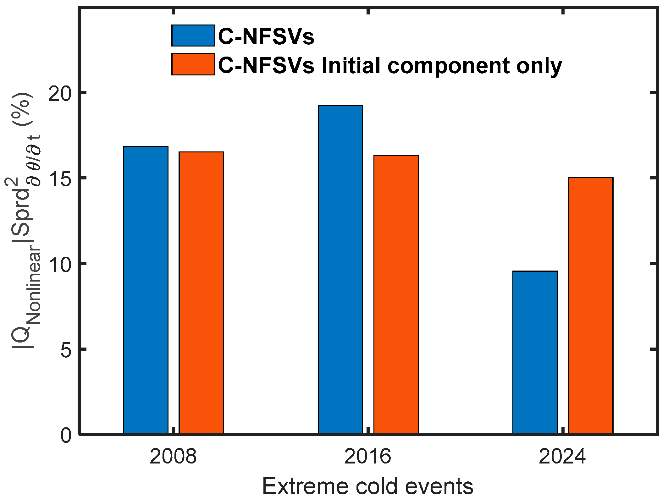
It should be noted that, because the ensemble spread is a nonlinear operator, some additional nonlinear terms appear on the right-hand side of the equation, and these terms are collectively represented by $Q_{nonlinear}$ in this study. To further evaluate the impact of the nonlinear term $Q_{nonlinear}$ on the interpretation of individual tendency terms, we quantified their relative magnitude by calculating the ratio of the nonlinear term to the total squared ensemble spread $Spr{d}^2\left({\displaystyle \frac{\partial \theta }{\partial t}}\right)$. The ratios were examined for the extreme cold events investigated in Table 1. The temporal evolution of this ratio is shown in Figure 1.

As shown in Figure 1, the nonlinear term $Q_{nonlinear}$ accounts for approximately 10–18% of the total squared ensemble spread across the investigated events for the C-NFSVs ensemble. This indicates that the nonlinear/residual term is not entirely negligible, but remains relatively small compared with the total uncertainty budget. Therefore, although the nonlinear term may introduce some uncertainty into the interpretation of individual tendency terms, it is unlikely to dominate the diagnosed sensitivities of the dynamical and physical processes.

Although the actual forecast uncertainty cannot be directly quantified during real-time forecasting, the C-NFSVs-based ensemble spread has been demonstrated to provide a reasonable approximation of forecast uncertainty in Hou et al. [19]. This suggests that the ensemble spreads associated with different terms in the potential temperature budget Equation (4) can be used as an approximation to evaluate their relative sensitivities to forecast uncertainty. Based on this assumption, we further focus on the cold periods identified by Hou et al. as being dominated by model uncertainty in terms of their forecast uncertainty [19] (see Table 1). For these cases, ensemble forecasts are generated using the full C-NFSVs as well as using only the initial components of the C-NFSVs. The effects of model-related processes are diagnosed from the differences in ensemble spreads of individual tendency terms between the full C-NFSVs and the experiments with only its initial component. This comparison allows us to assess how different temperature tendency components contribute to 2 m temperature forecast uncertainty over southern China under the influence of model uncertainty.

4. Contributions of Different Model Processes to 2 m Temperature Forecast Uncertainty Associated with Model Uncertainty

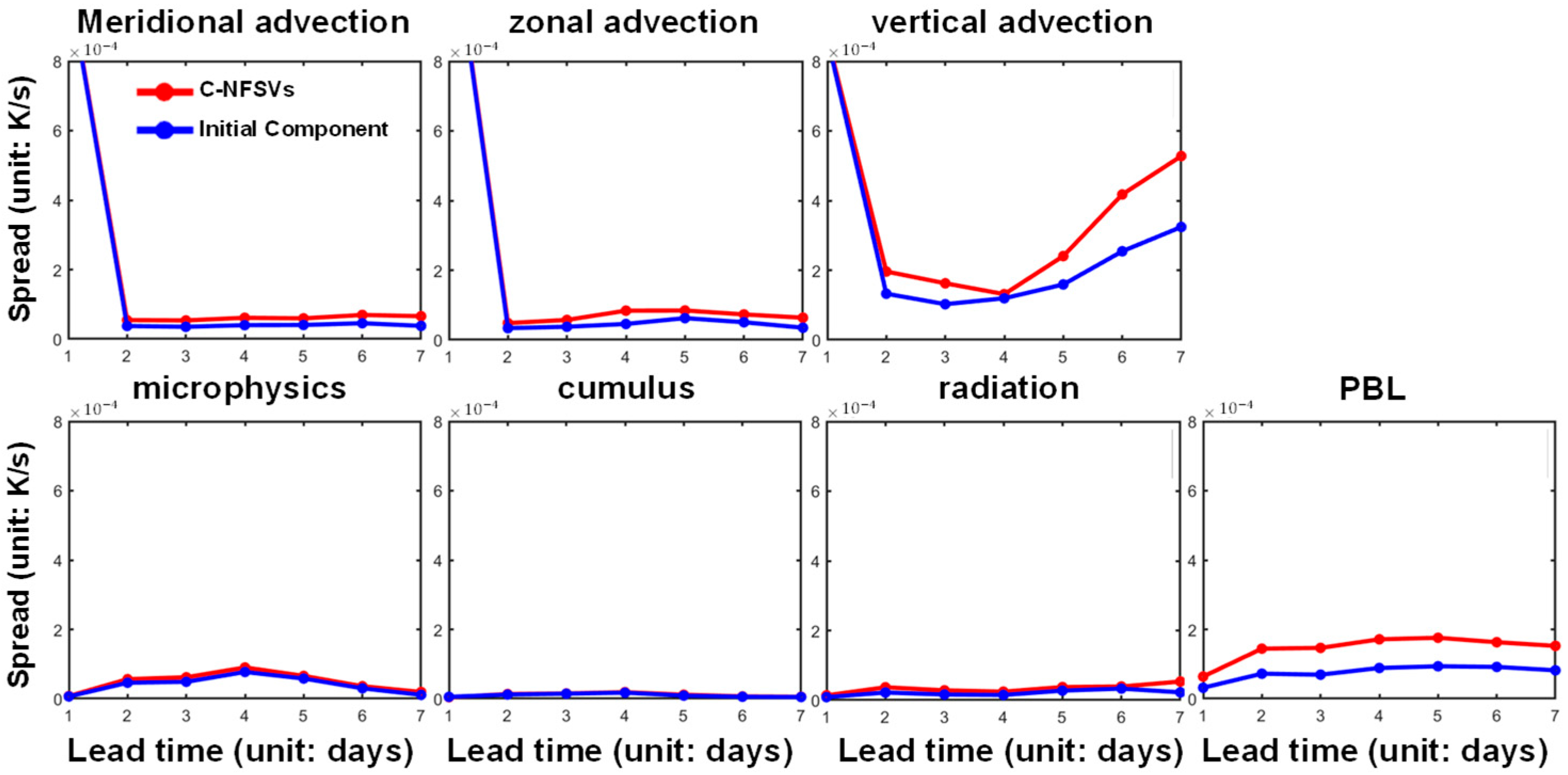
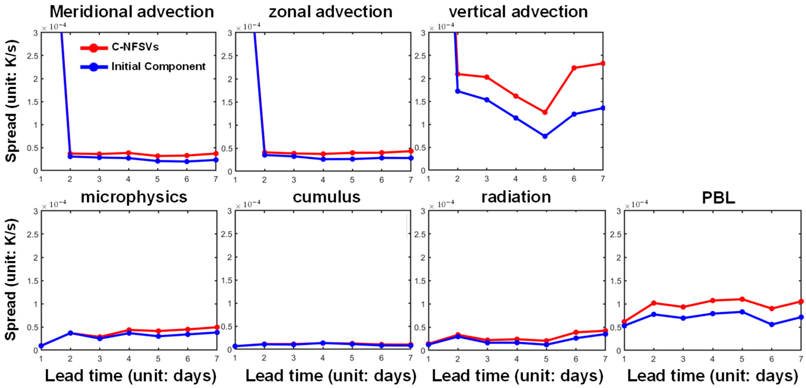
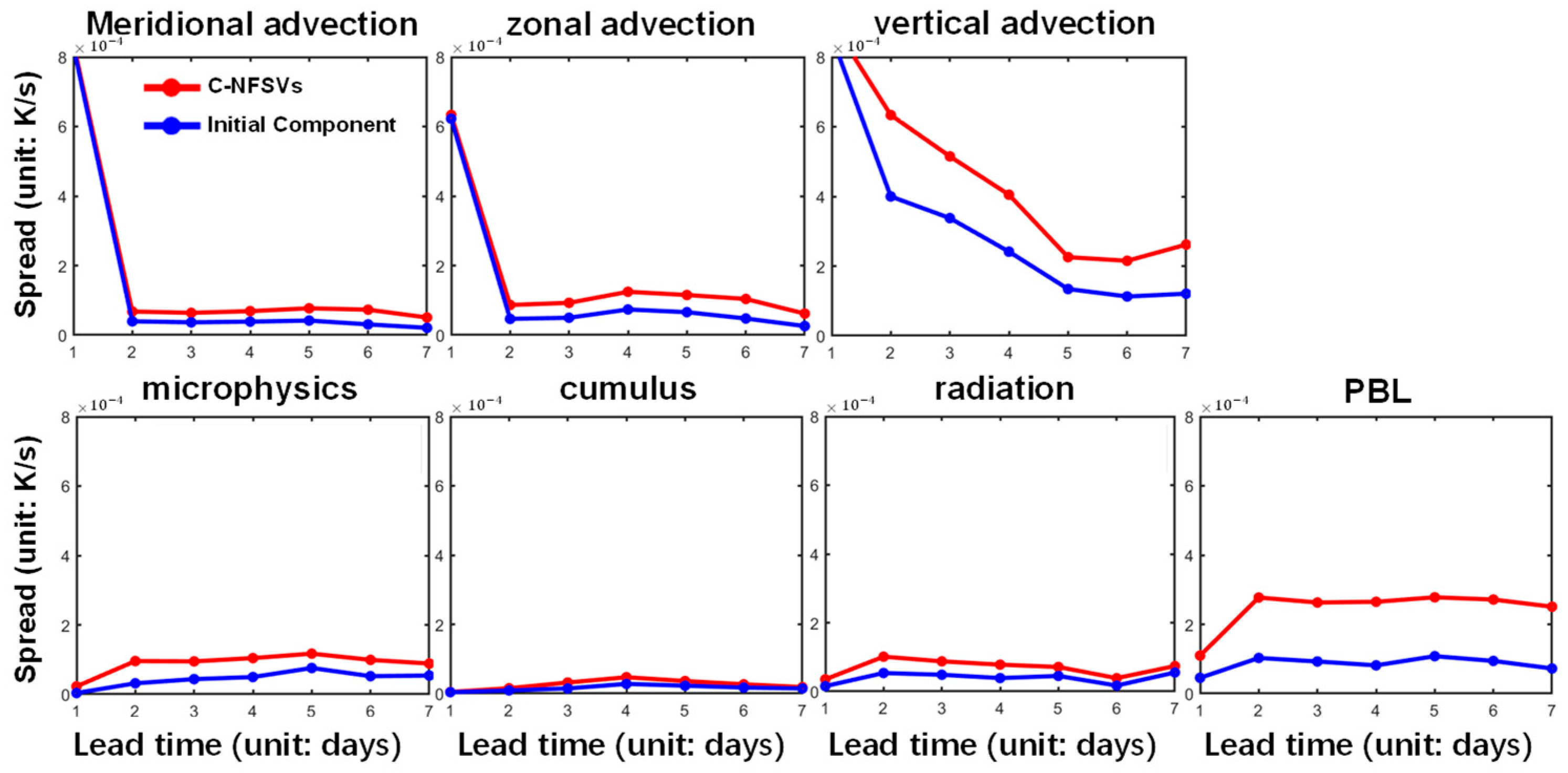
Among the cold periods within the 2008, 2016, and 2024 extreme cold events, those for which forecast uncertainty was dominated by model uncertainty were selected for the analysis presented in this study (Table 1). The temporal evolutions of the area-averaged ensemble spreads of different temperature tendency terms in Equation (5) over southern China are presented in Figure 2, Figure 3 and Figure 4.

As shown in Figure 2, Figure 3 and Figure 4, differences in ensemble spreads are found between the experiments using the complete C-NFSVs perturbations and those using only its initial components. Across the different extreme cold events, these differences are mainly concentrated in the vertical advection term and the planetary boundary layer (PBL) parameterization term. These results indicate that, among the model processes considered in the temperature tendency budget, the vertical transport and PBL parameterization processes make the largest contributions to model uncertainty-related 2 m temperature forecast uncertainty over southern China.

5. Discussion

The enhanced sensitivities of the vertical transport and PBL parameterization terms revealed in Section 4 provide some physical insights into the processes associated with model-related 2 m temperature forecast uncertainty. In the WRF model, the evolution of near-surface temperature is jointly influenced by resolved dynamical processes and subgrid-scale physical processes. Among these processes, the PBL scheme and vertical advection term represent two important mechanisms governing the vertical exchange of heat and momentum in the lower atmosphere. The PBL parameterization primarily represents turbulent mixing and vertical transport processes within the boundary layer, including the redistribution of heat and momentum through turbulent fluxes [25,34]. In contrast, the vertical advection term represents the vertical motion that contributes to the upward or downward transport of atmospheric thermal properties. Therefore, uncertainties in these two processes may be closely associated with changes in the evolution of the lowest model-layer potential temperature, which is closely related to the diagnosed 2 m temperature.

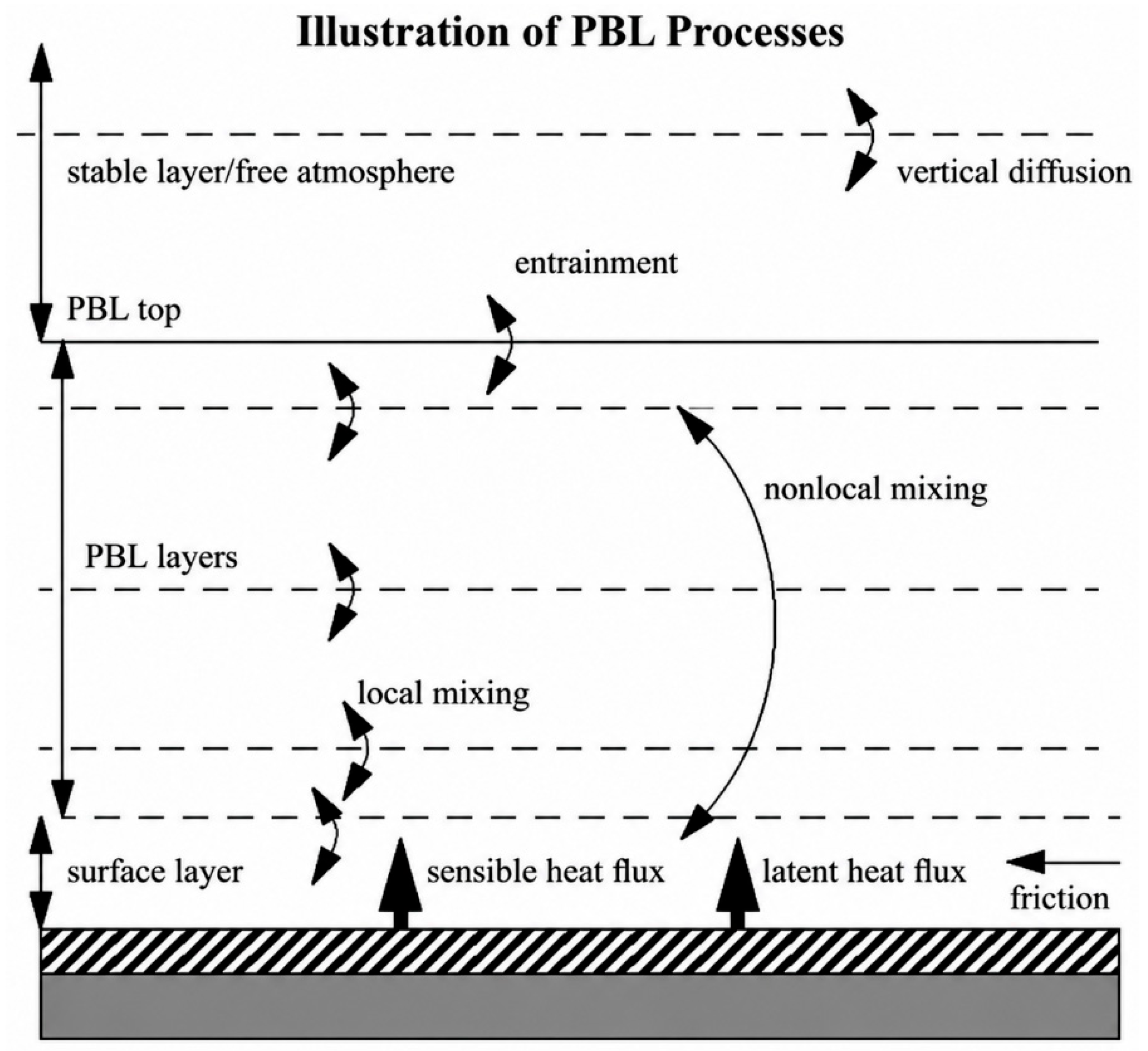
A possible explanation for the closely coupled effects of the PBL scheme and vertical advection term lies in the interaction between thermodynamic and dynamical processes in the lower atmosphere. Figure 5 provides a schematic illustration of the PBL processes represented in the WRF model. As discussed above, the PBL scheme describes the effects of subgrid-scale turbulent mixing and vertical exchanges of heat within the boundary layer. Uncertainties in these processes, such as those associated with atmospheric stability and turbulent mixing intensity, may modify the vertical redistribution of surface sensible heat fluxes and consequently introduce uncertainties into the lower-tropospheric thermal structure. Changes in the lowest-layer potential temperature may modify the atmospheric buoyancy state, which could influence the simulated vertical motion and potentially introduce uncertainties in vertical velocity. Although such thermal perturbations may also influence horizontal winds through dynamical adjustments, their impacts on horizontal temperature transport are expected to be weaker because horizontal advection is primarily controlled by synoptic-scale circulation and large-scale cold-air transport. Since the vertical advection term is directly related to vertical motion through $w\cdot {\displaystyle \frac{\partial \theta }{\partial z}}$, the thermal perturbations associated with PBL uncertainties may be linked to dynamical uncertainties in vertical advection. This potential coupling may provide a plausible physical interpretation of the simultaneous increase in ensemble spreads of the PBL term and the vertical advection term after introducing model perturbations. Furthermore, as a diagnostic near-surface variable, 2 m temperature is derived from the lowest atmospheric model state and surface-layer processes rather than directly predicted by the model. Its evolution therefore depends strongly on both the turbulent exchange of heat between the surface and atmosphere represented by PBL schemes and the transport of colder air from higher levels associated with vertical motion. When uncertainties exist in both processes, their combined effects may modify the lower-atmospheric thermodynamic balance and subsequently influence the evolution of 2 m temperature. It should be noted that the coupling between PBL processes and vertical advection proposed here represents a plausible physical interpretation of the experimental results rather than a mechanism directly demonstrated by the present analysis.

As a preliminary investigation, this study mainly provides a qualitative analysis of the potential impacts of uncertainties in vertical advection and PBL processes on 2 m temperature forecast uncertainty during extreme cold events. Since 2 m temperature is a diagnostic variable rather than a directly predicted model variable, the diagnosis was performed using the potential temperature tendency in the lowest model layer. Therefore, the identified sensitivities should be interpreted as the impacts of these processes on near-surface thermal evolution associated with T2m forecasts rather than a direct decomposition of T2m uncertainty. Furthermore, it should be noted that the identified sensitivity of PBL-related uncertainty is based on the MYJ PBL scheme adopted in the present WRF configuration and may depend on the specific physics configuration. Therefore, further investigations using alternative PBL schemes and model configurations are needed to assess the generality of this finding, better quantify the underlying mechanisms and relative impacts of these processes, and examine whether these results can be extended to other high-impact weather events. Nevertheless, the results presented here highlight the importance of further investigating the representation of these processes in numerical models, which may provide a potential direction for reducing forecast uncertainty associated with model errors and improving the prediction of 2 m temperature during extreme cold events.

6. Conclusions

For extreme cold events, the prediction of 2 m temperature closely linked to societal impacts remains a major challenge. Previous studies have shown that C-NFSVs-based ensemble forecasts can provide a reliable estimation of their forecast uncertainty and distinguish the relative contributions of initial and model errors to forecast uncertainty. However, the specific dynamical and physical parameterization processes responsible for model-related forecast uncertainty remain insufficiently understood. In this study, for the cold periods in the 2008, 2016, and 2024 extreme cold events, where model error was identified as the dominant source of forecast uncertainty, we further investigated the sensitivity of 2 m temperature forecast uncertainty to different dynamical and physical parameterization processes within the WRF model.

Ensemble forecasts generated with complete C-NFSVs perturbations were compared with those including only its initial component, and the differences between the two experiments were used to assess the sensitivity of forecast uncertainty to model perturbations. Specifically, since 2 m temperature is a diagnostic variable derived from atmospheric model states rather than a directly predicted model variable, the temperature tendency of the lowest model layer was used as a proxy to diagnose the sensitivity of different model processes to forecast uncertainty. This approximation is based on the fact that the potential temperature in the lowest model layer provides a representation of the near-surface atmospheric thermal state and is closely related to the evolution of 2 m temperature. However, it should be noted that the potential temperature does not exactly represent T2m, which is diagnostically derived considering surface conditions and near-surface atmospheric stratification.

The results indicate that the impacts of model uncertainty on 2 m temperature forecasts are not uniformly distributed among different temperature tendency terms. Among the processes considered, the vertical advection term and the PBL parameterization term exhibit the most pronounced differences between the two scenarios for the extreme cold events examined in this study, suggesting that 2 m temperature forecasts are particularly sensitive to uncertainties in these processes over southern China. A possible explanation is that the PBL parameterization and vertical advection jointly regulate the vertical exchange and redistribution of heat in the lower atmosphere. Uncertainties in PBL processes may modify the lower-tropospheric thermal structure and potentially influence vertical motion through thermodynamic–dynamic coupling, which provides a plausible explanation for the associated changes in vertical advection uncertainty. This interaction may explain the closely linked increases in ensemble spreads of these two temperature tendency terms when model perturbations are introduced.

Overall, this study provides a preliminary investigation into how uncertainties in different model processes are associated with model-related forecast uncertainty in extreme cold events. The results highlight the importance of further investigating the representation of vertical advection and PBL-related processes in the WRF model. Such efforts may provide further insights into the reduction in model-related forecast uncertainty and the improvement of 2 m temperature predictions during extreme cold events.

References

1. Wang, Z.; Ding, Y. Climate change of the cold wave frequency of China in the last 53 years and the possible rea-sons. Chin. J. Atmos. Sci. 2006, 30, 1068. (In Chinese) [Google Scholar]
2. Liu, W.; Huang, S.; Li, D.; Wang, C.; Zhou, X.; Chen, S. Spatiotemporal computing of cold wave characteristic in recent 52 years: A case study in Guangdong Province, South China. Nat. Hazards 2015, 79, 1257–1274. [Google Scholar] [CrossRef] [Scilit]
3. Ryti, N.R.I.; Guo, Y.; Jaakkola, J.J.K. Global association of cold spells and adverse health effects: A systematic re-view and meta-analysis. Environ. Health Perspect. 2016, 124, 12–22. [Google Scholar] [CrossRef] [Scilit] [PubMed]
4. Tao, S.Y.; Wei, J. Severe snow and freezing-rain in January 2008 in southern China. Clim. Environ. Res. 2008, 13, 337–350. (In Chinese) [Google Scholar]
5. Jiang, Q.; Ma, X.; Wang, F. Analysis of the January 2016 atmospheric circulation and weather. Meteorol. Mon. 2016, 42, 514–520. (In Chinese) [Google Scholar] [CrossRef]
6. Xu, R.; Zhang, T.H.; Rao, X.Q.; You, Y. Analysis of the December 2018 atmospheric circulation and weather. Meteorol. Mon. 2019, 45, 437–443. (In Chinese) [Google Scholar] [CrossRef]
7. Chi, X.; Ma, X.; Jiang, Q.; Yuan, Y.; Guan, L. Analysis of the December 2020 atmospheric circulation and weather. Meteorol. Mon. 2021, 47, 381–388. (In Chinese) [Google Scholar] [CrossRef]
8. Xie, C.; Gui, H.; You, Y. Analysis of the January 2024 atmospheric circulation and weather. Meteorol. Mon. 2024, 50, 514–520. (In Chinese) [Google Scholar] [CrossRef]
9. Xu, X.; Zhang, F. Analysis of the February 2024 atmospheric circulation and weather. Meteorol. Mon. 2024, 50, 642–648. (In Chinese) [Google Scholar] [CrossRef]
10. Yu, X.; Fei, H.; Wang, X. Some issues concerning the large area rainstorm, snowstorm, sleet, freezing rain and severe convection event over China from 17 to 23 February 2024. Meteorol. Mon. 2024, 50, 1033–1042. (In Chinese) [Google Scholar] [CrossRef]
11. Lorenz, E.N. The predictability of a flow which possesses many scales of motion. Tellus 1969, 21, 289. [Google Scholar] [CrossRef] [Scilit]
12. Lorenz, E.N. Atmospheric predictability experiments with a large numerical model. Tellus 1982, 34, 505. [Google Scholar] [CrossRef] [Scilit]
13. Vannitsem, S.; Toth, Z. Short-term dynamics of model errors. J. Atmos. Sci. 2002, 59, 2594–2604. [Google Scholar] [CrossRef] [Scilit]
14. Nicolis, C.; Perdigao, R.A.; Vannitsem, S. Dynamics of prediction errors under the combined effect of initial con-dition and model errors. J. Atmos. Sci. 2009, 66, 766–778. [Google Scholar] [CrossRef] [Scilit]
15. Persson, A.; Grazzini, F. User guide to ECMWF forecast products. Meteorol. Bull. 2007, 3. 153. [Google Scholar]
16. Préaux, D.; Dombrowski-Etchevers, I.; Gouttevin, I.; Seity, Y. On the proper use of screen-level temperature measurements in weather forecasting models over mountains. Geosci. Model Dev. 2025, 18, 8723–8749. [Google Scholar] [CrossRef] [Scilit]
17. Palmer, T.N.; Shutts, G.J.; Hagedorn, R.; Doblas-Reyes, F.J.; Jung, T.; Leutbecher, M. Representing model uncer-tainty in weather and climate prediction. Annu. Rev. Earth Planet. Sci. 2005, 33, 163–193. [Google Scholar] [CrossRef] [Scilit]
18. Du, J.; Berner, J.; Buizza, R.; Charron, M.; Houtekamer, P.; Hou, D.; Jankov, I.; Mu, M.; Wang, X.; Wei, M.; et al. Ensemble methods for meteorological predictions. In Handbook of Hydrometeorological En-semble Forecasting; Springer: Berlin, Germany, 2018; pp. 1–52. [Google Scholar] [CrossRef] [Scilit]
19. Hou, Y.; Duan, W.; Han, Z. Recognizing sources of forecast uncertainty in extreme cold events: The C-NFSVs method. Adv. Atmos. Sci. 2026, 43, 1362–1378. [Google Scholar] [CrossRef] [Scilit]
20. Duan, W.; Ma, J.; Vannitsem, S. An ensemble forecasting method for dealing with the combined effects of the initial and model errors and a potential deep learning implementation. Mon. Weather Rev. 2022, 150, 2959–2976. [Google Scholar] [CrossRef] [Scilit]
21. Skamarock, W.C.; Klemp, J.B.; Dudhia, J.; Gill, D.O.; Barker, D.M.; Duda, M.G.; Huang, X.-Y.; Wang, W.; Powers, J.G. A Description of the Advanced Research WRF Version 3; NCAR Technical Note NCAR/TN-475+STR; National Center for Atmospheric Research: Boulder, CO, USA, 2008. [Google Scholar]
22. Thompson, G.; Field, P.R.; Rasmussen, R.M.; Hall, W.D. Explicit forecasts of winter precipitation using an improved bulk microphysics scheme. Part II: Implementation of a new snow parameterization. Mon. Weather Rev. 2008, 136, 5095–5115. [Google Scholar] [CrossRef] [Scilit]
23. Iacono, M.J.; Delamere, J.S.; Mlawer, E.J.; Shephard, M.W.; Clough, S.A.; Collins, W.D. Radiative forcing by long-lived greenhouse gases: Calculations with the AER radiative transfer models. J. Geophys. Res. 2008, 113, D13103. [Google Scholar] [CrossRef] [Scilit]
24. Tiedtke, M. A comprehensive mass flux scheme for cumulus parameterization in large-scale models. Mon. Weather Rev. 1989, 117, 1779–1800. [Google Scholar] [CrossRef] [Scilit]
25. Janjić, Z.I. The step-mountain Eta coordinate model: Further developments of the convection, viscous sublayer, and turbulence closure schemes. Mon. Weather Rev. 1994, 122, 927–945. [Google Scholar] [CrossRef] [Scilit]
26. Global Forecast System (GFS). Available online: https://www.ncei.noaa.gov/products/weather-climate-models/global-forecast (accessed on 13 August 2026).
27. Vannitsem, S. The role of scales in the dynamics of parameterization uncertainties. J. Atmos. Sci. 2006, 63, 1659–1671. [Google Scholar] [CrossRef] [Scilit]
28. Birgin, E.G.; Martínez, J.M.; Raydan, M. Nonmonotone spectral projected gradient methods on convex sets. SIAM J. Optim. 2000, 10, 1196–1211. [Google Scholar] [CrossRef] [Scilit]
29. Yang, G.M.; Kong, Q.; Mao, D.Y.; Zhang, F.H.; Kang, Z.M.; Zong, Z.P. Analysis of the long-lasting cryogenic freezing rain and snow weather in the beginning of 2008. Acta Meteorol. Sin. 2008, 66, 836–849. (In Chinese) [Google Scholar]
30. Zhao, S.; Sun, J. Multi-scale systems and conceptual model on freezing rain and snow storm over southern China during January–February 2008. Clim. Environ. Res. 2008, 13, 351–367. (In Chinese) [Google Scholar]
31. Zhou, Q.; Gao, S.; Sun, X. Effects of the Upstream Temperature Anomaly on Freezing Rain and Snowstorms over Southern China in Early 2008. J. Meteorol. Res. 2016, 30, 694–705. [Google Scholar] [CrossRef] [Scilit]
32. Wang, D.; Lv, C.; Li, Y.; Wang, F.; Zhang, N.; Jiang, Z.; Li, Y.; Chen, J.; Wang, Y.; Song, X.; et al. A preliminary analysis of features and causes of the snow storm event over the southern areas of China in January 2008. Acta Meteorol. Sin. 2009, 23, 374–386. [Google Scholar]
33. Skamarock, W.C.; Klemp, J.B. A time-split nonhydrostatic atmospheric model for weather research and fore-casting applications. J. Comput. Phys. 2008, 227, 3465–3485. [Google Scholar] [CrossRef] [Scilit]
34. Mesinger, F. Forecasting upper tropospheric turbulence within the framework of the Mellor-Yamada 2.5 closure. Res. Activ. Atmos. Oceanic Mod. 1993, 18, 4.28–4.29. [Google Scholar]
Figure 1. The temporal-mean ratio of the nonlinear term Q n o n l i n e a r to the total squared ensemble spread S p r d 2 ∂ θ ∂ t during different extreme cold events. The blue and red bars denote the C-NFSVs ensemble and the ensemble using only the initial component of C-NFSVs, respectively, for the 2008, 2016, and 2024 extreme cold events.
Atmosphere 17 00829 g001
Figure 2. Temporal evolution of the ensemble spread of potential temperature tendency terms among ensemble members associated with different dynamical processes and physical parameterization schemes, averaged over three forecast periods that are sensitive to model uncertainty during the 2008 extreme cold event (i.e., 20080115T00–0122T00, 20080122T00–0129T00, and 20080128T00–0204T00). The red lines denote ensemble forecasts generated by superimposing both initial and model perturbations derived from the C-NFSVs, whereas the blue lines represent ensemble forecasts generated by superimposing only the initial perturbation component of the C-NFSVs. The differences between the two ensembles reflect the contribution of model-related uncertainties to the spread of individual tendency terms.
Atmosphere 17 00829 g002
Figure 3. Same as Figure 2, but for the cold period during the 2016 extreme low-temperature event (i.e., 20160118T00-20160125T00).
Atmosphere 17 00829 g003
Figure 4. Same as Figure 2, but for the averaged results of the two cold periods during the 2024 extreme low-temperature event (i.e., 20240210T00-0217T00 and 20240216T00-0223T00).
Atmosphere 17 00829 g004
Figure 5. Schematic diagram illustrating the PBL process in the WRF model, adapted from the WRF Physics and Dynamics tutorial (NCAR-MMM, available at: https://www.youtube.com/watch?v=NPsotmEqTBw (accessed on 13 August 2026)).
Atmosphere 17 00829 g005