The Mahalanobis Distance as a Multivariate Performance Metric for Selecting Physics Parameterizations in Meteorological Simulations

Abstract

Selecting physics parameterizations for meteorological simulations is typically guided by univariate metrics, which are computed separately for each variable and station and frequently yield contradictory rankings and force subjective decisions. Although the Mahalanobis distance (MD) has previously been used for multivariate analysis, to the best of our knowledge, it has not previously been used as a decision criterion for selecting physics parameterizations in meteorological simulations. This study proposes the MD as a single multivariate performance metric that is dimensionless, invariant to measurement scales, and corrects for inter-variable correlations. The framework was demonstrated using 40 meteorological simulations combining microphysics, radiation, surface-layer, planetary boundary layer, and cumulus schemes, evaluated against hourly observations of temperature, relative humidity, and wind at surface stations in the Biobío region, south-central Chile. The traditional univariate metrics nominated different optimal configurations depending on the variable and station. In contrast, the MD identified a single configuration attaining the minimum distance at three of the four stations and the minimum cross-station mean, and revealed that performance was governed primarily by the surface-layer/PBL pairing rather than by microphysics or radiation choices. The MD thus provides an objective, reproducible, and easily interpretable criterion for parameterization selection, directly applicable to meteorological inputs for air quality modeling.

1. Introduction

Air quality models (AQMs) are essential tools for forecasting local pollution episodes and supporting environmental policies. Simulated meteorology plays a decisive role among their inputs; better adjustment of near-surface temperature (T2), relative humidity (RH), wind speed (WS), and wind direction (WD) reduces biases in the transport, dispersion, and photochemical transformation of air pollutants [1,2]. Meteorological models represent complex interactions between the atmosphere and land and ocean surfaces through a suite of physics parameterizations—microphysics, radiation, surface layer, land surface, planetary boundary layer (PBL), and cumulus schemes—whose combination must be tuned for each region and application [3].

Several studies have evaluated the performance of simulated meteorological variables under different parameterizations to identify suitable configurations for regional applications [4,5,6,7,8,9]. In these studies, the selection of the final model configuration was typically supported by comparisons with observational datasets and established performance criteria, thereby providing an objective basis for assessing and reducing uncertainties associated with the numerical simulations. Model performance was generally evaluated separately for each meteorological variable using established statistical metrics, including the root mean square error (RMSE), correlation coefficient (r), fraction of predictions within a factor of two (FAC2), and index of agreement (IOA). Additionally, one of the most referenced studies is the report by Emery et al. [10] which proposed a range of acceptance for meteorological simulation studies and derived their thresholds from a suite of meteorological mesoscale simulations conducted for two Texas ozone episodes. The proposed variable-by-variable acceptance benchmarks are as follows. For T2: mean bias (MB) ≤ ±0.5 K, mean gross error (MGE) < 2.0 K, RMSE < 2.0 K, and IOA ≥ 0.8. For RH: MB ≤ ±10%, MGE < 20%, RMSE < 20%, and IOA ≥ 0.6. For WS: MB ≤ ±0.5 m s⁻¹, MGE < 2.0 m s⁻¹, RMSE < 2.0 m s⁻¹, and IOA ≥ 0.6. Finally, for WD: MB ≤ ±10°, MGE < 30°. However, when a meteorological simulation meets the recommended acceptance criteria for some variables or monitoring locations but not for others, the procedure for selecting a single best parameterization scheme is often not straightforward.

Other integrated evaluation tools, such as Taylor diagrams, the distance between the indices of simulation and observation (DISO), and composite efficiency metrics, have been proposed to summarize different aspects of model performance [11,12]. However, they are generally applied to individual variables and therefore still require an additional aggregation rule when several meteorological variables and stations must be evaluated jointly. This situation motivates the use of a multivariate criterion capable of integrating the performance across several variables and monitoring stations into a single decision framework.

The limitations of applying performance measures to individual variables lie mainly in the difficulty of choosing a forecasting model that simultaneously compares k variables. Some contradictory cases in different variables can be obtained, which leads to subjective judgments in decision-making. Moreover, the Mahalanobis distance (MD), which is a dimensionless measure, can be useful for reducing uncertainties and difficulties in determining the best configuration for meteorological simulation studies.

The Mahalanobis distance is a generalization of the Euclidean distance between k-dimensional vectors [13]. This metric is characterized by considering the scale and correlation of the vector components such that they do not affect distance. It has been used to detect multivariate outliers [14] and perform classification in random samples and time series [15]. The Mahalanobis distance is defined as

$$d_M\left(x,y\right)=\sqrt{{\left(x-y\right)}^{\mathrm{T}}M\left(x-y\right)}\hspace{1em}x,y \in {\mathbb{R}}^k,\hspace{1em}M \in {\mathbb{R}}^{k x k}$$

(1)

where $x$ and $y$ are two k-dimensional vectors, and $M$ is a k × k symmetric positive-definite matrix. Consequently, d_M(x, y) satisfies the properties of a valid distance: (i) positivity, (ii) uniqueness, (iii) symmetry, and (iv) triangular inequality.

Suppose we have the observations x_i, y_i ∈ $\mathbb{R}$^k, i = 1, …, n, where n is the number of valid paired time intervals and each vector contains the k variables at observation i. Let X = (x₁, …, x_n)^T and Y = (y₁, …, y_n)^T, where the superscript T denotes the transpose operator. Consequently, X and Y are n × k matrices, with each row corresponding to one observation and each column corresponding to one variable. Here, n is the number of valid paired time steps.

Considering the differences D_i = x_i − y_i, $i=1$,…, $n$, the average difference vector is defined as follows:

$$\overline{D}={\displaystyle \frac{1}{n}}{\displaystyle \sum _{i=1}^n}{D}_i$$

(2)

$\overline{D}$ corresponds to the average difference between X and Y. Additionally, the variance and covariance matrix (S) of the differences between X and Y is defined as follows:

$$S={\displaystyle \frac{1}{n-1}}{\displaystyle \sum _{i=1}^n}(D_i-\overline{D}){(D_i-\overline{D})}^{{\rm T}}$$

(3)

Thus, the following three cases can be considered.

• M₁ = I_k (the identity matrix of order k)
• M₂ = (diag(S))⁻¹
• M₃ = S⁻¹

Case M₁ corresponds to the Euclidean distance, which is equivalent to the RMSE. Case M₂ corresponds to the Euclidean distance after standardizing the error components by their standard deviations, thus correcting for differences in scale but treating the components as uncorrelated. Case M₃ also accounts for the dependence between the error components. These correlated discrepancies are not treated as independent contributions to the overall distance.

Unlike an average of independently computed univariate performance measures, such as the mean IOA, the Mahalanobis distance jointly and explicitly evaluates the multivariate error vector by accounting for the dependence among its components through the covariance matrix.

Thus, the distance between x_i and y_i is denoted by d_i, which is given by the following equation:

$$d_i=d_M\left(x_i,y_i\right)=\sqrt{{\left(x_i-y_i\right)}^{\mathrm{T}}{S}^{-1}\left(x_i-y_i\right)},\hspace{1em}M=S^{-1}$$

(4)

The resulting vector d = (d₁, … d_n)^T collects the n hourly Mahalanobis distances between the corresponding observed and simulated vectors $x_i$ and $y_i$, respectively. From the distance vector d, we can identify the time points with the largest discrepancies between observed and simulated vectors. Assuming normality, all points that satisfy $d_i^2$ > ${\chi }_{1-\alpha ,k}^2$ are considered far away, where ${\chi }_{1-\alpha ,k}^2$ denotes the (1 − α)-quantile of a chi-squared distribution with k degrees of freedom, k is the number of variables, and α is the significance level. For five variables, $k=5$, and using the conventional significance level $\alpha =0.05$, the corresponding threshold for the Mahalanobis distance is $\sqrt{{\chi }_{\mathrm{0.95,5}}^2}=3.33$. This value provides a reference threshold for identifying large multivariate discrepancies between the simulated and observed vectors.

On the other hand, the distance vector d can also define a unique metric representing the separation between X and Y as follows:

$${∆}^2\left(X,Y\right)={\displaystyle \frac{1}{n}}\sum _{i=1}^n{d}_i^2={\displaystyle \frac{1}{n}}\sum _{i=1}^n{\mathrm{d}}_{\mathrm{M}}^2\left(x_i,y_i\right)$$

(5)

The distance $∆(X,Y)$ defined by Equation (5) is a global measure of the separation between X and Y. Consequently, assuming squared individual Mahalanobis distances have a mean k and variance 2k. Assuming independent observations, ${∆}^2(X,Y)$ has a mean k and variance ${\displaystyle \frac{2k}{n}}$. For sufficiently large n, the central limit theorem provides the following approximate upper reference threshold:

$$∆\left(X,Y\right)>\sqrt{k+z_{1-\alpha }\sqrt{{\displaystyle \frac{2k}{n}}}}$$

(6)

where $z_{1-\alpha }$ denotes the (1 − α)-quantile of the standard normal distribution. This threshold provides a reference for interpreting the magnitude of the global distance under the independence assumption.

In several applications, including air quality, several indicators (variables) are observed over time at one station (fixed point), and the same variables are frequently observed at multiple stations (several fixed geographical points). Since the squared distance defined in Equation (5) is unitless and assuming that there are m stations, we can measure the total discrepancy between a model and the observed values by considering the average of the square root of the defined square distances in Equation (5).

The Mahalanobis distance has been applied to evaluate different topics. González-Arteaga et al. [16] used MD to construct a cardinal dissensus measure for group decision-making, where each agent is represented by a vector of quantitative evaluations over several alternatives. They considered five correlated macroeconomic variables forecast by five institutions, demonstrating the use of MD as a covariance-aware multivariate discrepancy measure. Kumar et al. [17] used MD as a data-driven diagnostic indicator for electronic products by combining multiple normalized and correlated performance parameters into a single system-health measure rather than evaluating each parameter separately. Their approach established a healthy baseline and probabilistic thresholds for transformed MD values using Box–Cox and control-chart methods, and then used residual analysis to isolate the parameter responsible for the fault, demonstrating the usefulness of MD for multivariate monitoring of correlated variables.

Using a similar approach, Puentes et al. [18] applied MD in a bivariate regression framework to forecast daily fine (PM_2.5) and respirable (PM₁₀) particulate matter levels in Santiago, Chile, using it as a diagnostic tool to assess bivariate outliers and the suitability of the assumed data distribution. Their application illustrated how MD can support environmental model diagnostics by identifying atypical cases in correlated response variables, including episodes associated with extreme aerosol levels or large rainfall events.

A similar rationale has been extended from local air-quality diagnostics to industrial process monitoring at the national scale. Tao et al. [19] evaluated the performance of municipal solid waste incinerators at the national level in China by applying MD to monthly multivariate flue-gas emission profiles to identify potential operational errors and risks. They detected 31 outliers in nine of the 37 evaluated plants, even though the monthly average values of regulated pollutants were within the national emission limits. This application is relevant because it shows that MD can reveal hidden abnormal behavior in apparently normal environmental datasets and can support operational decision-making by linking multivariate anomalies to process-stability factors, such as the frequency of waste-load changes. Additionally, an ensemble learning approach based on multiple MD metrics has been applied to detect structural damage in civil engineering structures while mitigating the confounding effects of environmental variability [20].

To the best of the authors’ knowledge, no studies have used MD for meteorological simulations. This study aimed to analyze MD as a robust statistical indicator to obtain the best meteorological simulation performance when various parameterization schemes are evaluated. This proposal standardizes each variable according to its measurement scale and corrects the effect of the correlation between variables, which allows us to identify the real distance between the simulation and the observed values.

2. Materials and Methods

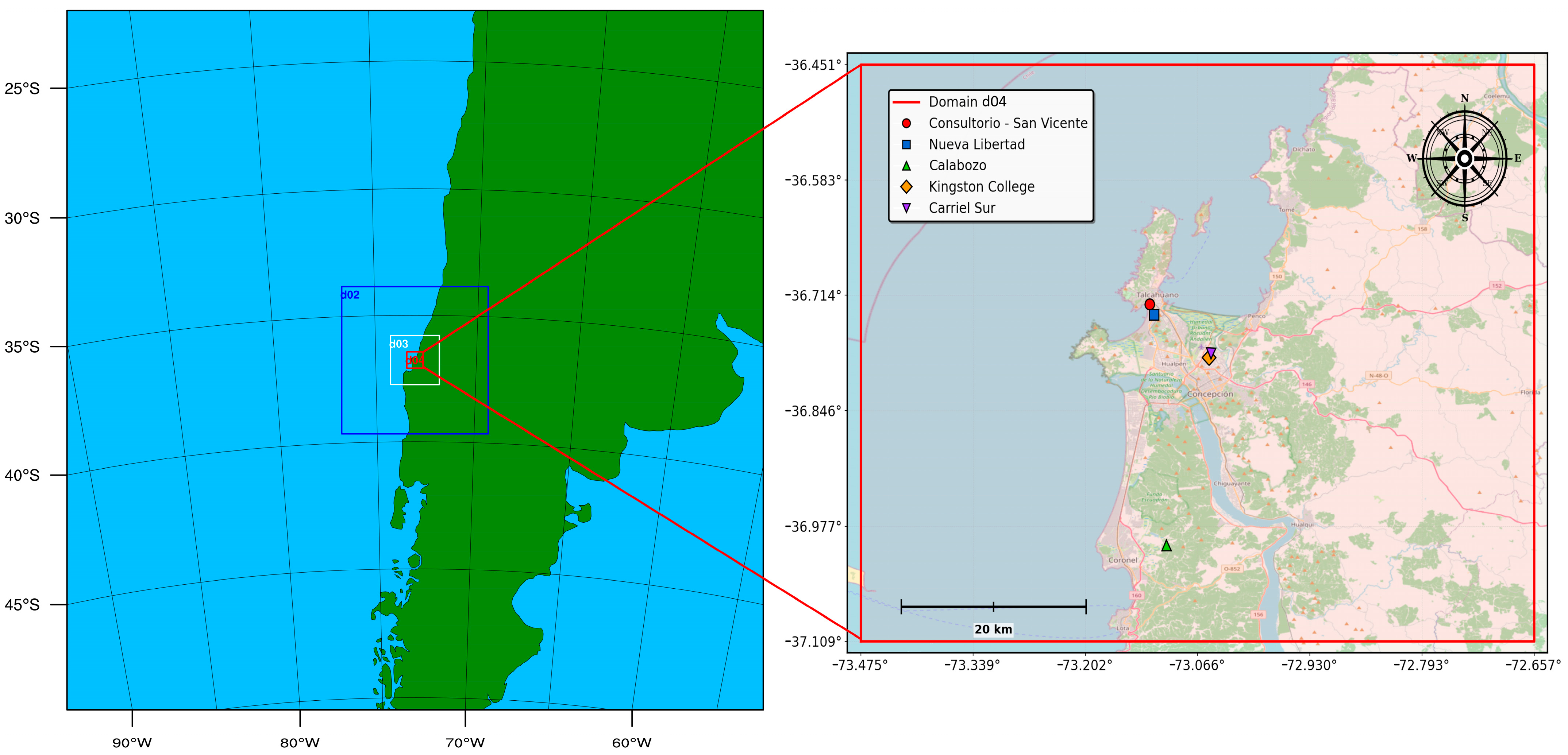
This study used the Weather Research and Forecasting (WRF) model version 4.1 [21] to perform meteorological simulations. This is one of the most commonly used models in recent years, with several improvements. The case study was conducted over the Bio Bio region in south-central Chile, a coastal and topographically complex area where near-surface meteorological fields are relevant for subsequent air-quality applications. The modeling system consisted of four one-way nested domains centered near the Carriel Sur meteorological station, operated by the Chilean Meteorological Office (DMC) in the Hualpén municipality (36.78055° S, 73.06639° W). The horizontal grid resolutions were 27, 9, 3, and 1 km for domains d01 through d04, respectively. Domain d01 contained 115 × 115 grid cells, whereas domains d02, d03, and d04 contained 73 × 73 grid cells. The WRF domain configuration followed a modeling setup previously applied in studies conducted in Chile [22,23]. The spatial configuration of the domains is shown in Figure 1.

The simulation case started on 23 August, from 00:00 until 14 September, 2019, at 21:00. The spin-up period considered was 2 days. This is why the period of analysis for the final decisions started on 25 August.

Parameterization schemes were selected to define a controlled and computationally feasible WRF sensitivity experiment rather than an exhaustive factorial evaluation of all available physical options. The selected configurations included commonly used and physically distinct schemes for microphysics, radiation, surface layer processes, land surface exchange, planetary boundary layer dynamics, and cumulus parameterization. This design provided a representative set of alternative model configurations with different treatments of near-surface meteorology, vertical mixing, cloud processes and radiative transfer. The purpose was to generate a sufficiently diverse ensemble of simulations for evaluating the Mahalanobis distance as a multivariate decision criterion across meteorological variables and monitoring stations. The initial and lateral boundary conditions were obtained from the NCEP Final Analysis dataset (GFS-FNL, ds.082) available from the NCAR Research Data Archive [24].

The parameterizations evaluated are listed in

Table 1. Physical parameterization schemes analyzed.

Parameterization	Variable	Option
Microphysiscs	mp_physics	1 Kessler Scheme 2 Purdue Lin Scheme 3 WRF Single–moment 3–class Scheme 4 WRF Single–moment 5–class Scheme 6 WRF Single–moment 6–class Scheme 7 Goddard Scheme 8 Thompson Scheme 9 Milbrandt–Yau Double Moment Scheme
Radiation Longwave/Shortwave	ra_lw_physics/ra_sw_physics	1 RRTM Longwave Scheme/Dudhia Shortwave Scheme 3 CAM Shortwave and Longwave Schemes 4 RRTMG Shortwave and Longwave Schemes
Surface Layer	sf_sfclay_physics	3 NCEP Global Forecast System Scheme 4 QNSE Scheme 5 MYNN Scheme 91 MM5 Similarity Scheme
Land Surface	sf_surface_physics	2 Unified Noah Land Surface Model
Planet Boundary Layer	bl_pbl_physics	1 Yonsei University Scheme (YSU) 3 NCEP Global Forecast System Scheme 4 Quasi–normal Scale Elimination (QNSE) Scheme 5 Mellor–Yamada Nakanishi Niino (MYNN) Level 2.5 6 Mellor–Yamada Nakanishi Niino (MYNN) Level 3 8 Bougeault–Lacarrere Scheme (BouLac)
Cumulus	cu_physics	1 Kain–Fritsch Scheme 2 Moisture–advection–based Trigger for Kain–Fritsch Cumulus Scheme 3 RH–dependent Additional Perturbation to option 1 for the Kain-Fritsch Scheme

.

In this study, we evaluated a controlled sensitivity subset of WRF physics parameterization combinations, rather than a complete factorial combination of all available schemes, resulting in 40 runs. Details are shown in

Table 2. Combinations of parameterizations for the simulations.

Run	mp_physics	ra_lw_physics/ra_sw_physics	sf_sfclay_physics	bl_pbl_physics	cu_physics
1	3	1	91	1	1
2	3	1	91	1	2
3	3	1	91	1	3
4	1	4	91	1	1
5	3	4	91	1	1
6	1	1	91	1	1
7	2	1	91	1	1
8	4	1	91	1	1
9	7	1	91	1	1
10	8	1	91	1	1
11	9	1	91	1	1
12	1	1	91	1	3
13	2	1	91	1	3
14	4	1	91	1	3
15	7	1	91	1	3
16	8	1	91	1	3
17	9	1	91	1	3
18	1	4	3	3	1
19	3	4	3	3	1
20	7	1	3	3	3
21	7	1	4	4	3
22	7	1	5	5	3
23	7	1	5	6	3
24	7	1	91	8	3
25	6	1	3	3	3
26	6	1	4	4	3
27	6	1	5	5	3
28	6	1	5	6	3
29	6	1	91	8	3
30	7	3	3	3	3
31	7	4	3	3	3
32	6	3	3	3	3
33	6	4	3	3	3
34	7	4	91	1	1
35	7	4	3	3	1
36	6	4	91	1	1
37	6	4	3	3	1
38	6	1	91	1	1
39	6	1	91	1	2
40	6	1	91	1	3

. Consequently, the selected configuration should be interpreted as the best-performing option among the tested schemes, rather than as a universally optimal configuration for the region.

The data obtained from the simulation were compared with those of five monitoring stations, four of which belong to the National Air Quality Information System (SINCA in Spanish) [25] and the other to the Chilean Meteorological Office (DMC in Spanish) [26], as detailed in

Table 3. Meteorological variables at each station.

Station	Location	Variable with Hourly Available Data	Latitude	Longitude
Consultorio San Vicente	Talcahuano	T2, RH, WS, WD	36.724° S	73.124° W
Nueva Libertad	Talcahuano	WS, WD	36.736° S	73.119° W
Calabozo	Coronel	T2, RH, WS, WD	36.999° S	73.104° W
Kingston College	Concepción	T2, RH, WS, WD	36.785° S	73.052° W
Carriel Sur	Hualpén	T2, RH, WS, WD	36.780° S	73.050° W

.

The wind direction was treated as a unit vector, with components in the x-axis (Dir-x) and y-axis (Dir-y).

All five evaluation stations lie within d04 (Figure 1) and are therefore resolved at a 1 km grid spacing. For each monitoring station, the simulated value was extracted from the d04 grid cell containing the station location and paired with the corresponding hourly observation. The observed and simulated data were paired at an hourly resolution using common valid timestamps, after excluding the spin-up period. Missing observational records were excluded from the paired comparisons.

The univariate metrics included the FAC2, RMSE, and IOA. FAC2 and IOA were interpreted as skill metrics, with higher values indicating better agreement, whereas RMSE was interpreted as an error metric, with lower values indicating better agreement. FAC2 was not applied to the absolute temperature because a factor of two criterion is not physically meaningful for this variable. The mathematical definitions of these metrics are provided in Appendix A, Equations (A1)–(A3).

These conventional metrics were used as diagnostic indicators to illustrate how the preferred WRF configuration varied depending on the selected variable, station, and the performance metric. The final multivariate ranking of the tested configurations was performed using the Mahalanobis distance with $k=5$.

3. Results

The following results are presented by comparing the values obtained from the simulation in WRF and the observed data at monitoring stations using the different statistical metrics mentioned above by decomposing the results into two sections. The first section presents traditional univariate performance measures. The second section presents the performance of the meteorological simulation using the Mahalanobis distance as a single decision tool. It should be noted that the relevance of looking at a single statistical metric that immediately compares simulated and observed data for all studied meteorological variables is more convenient than looking for metrics that only consider one performance variable at a time.

3.1. Performance Indicators for Single Variables

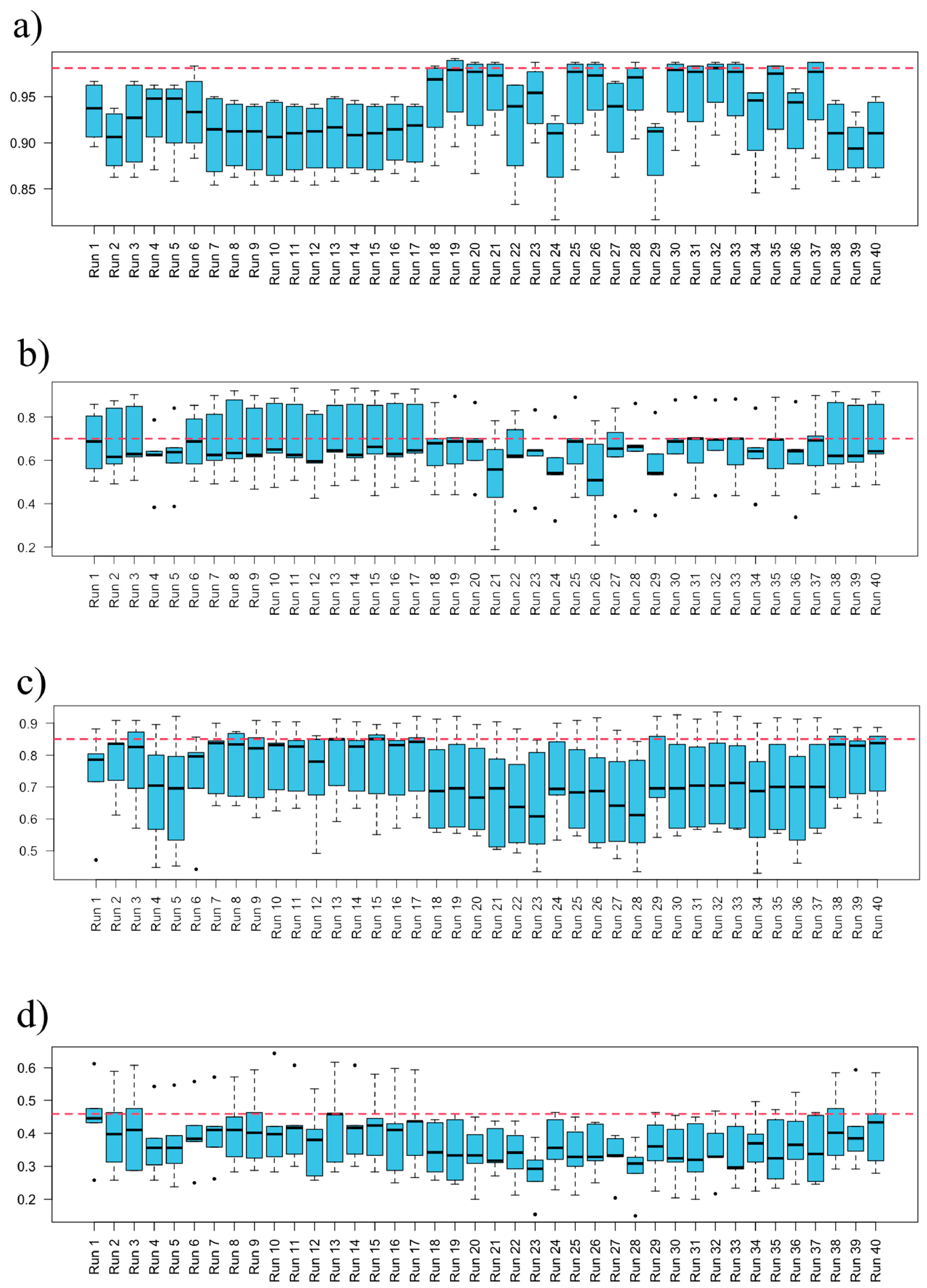
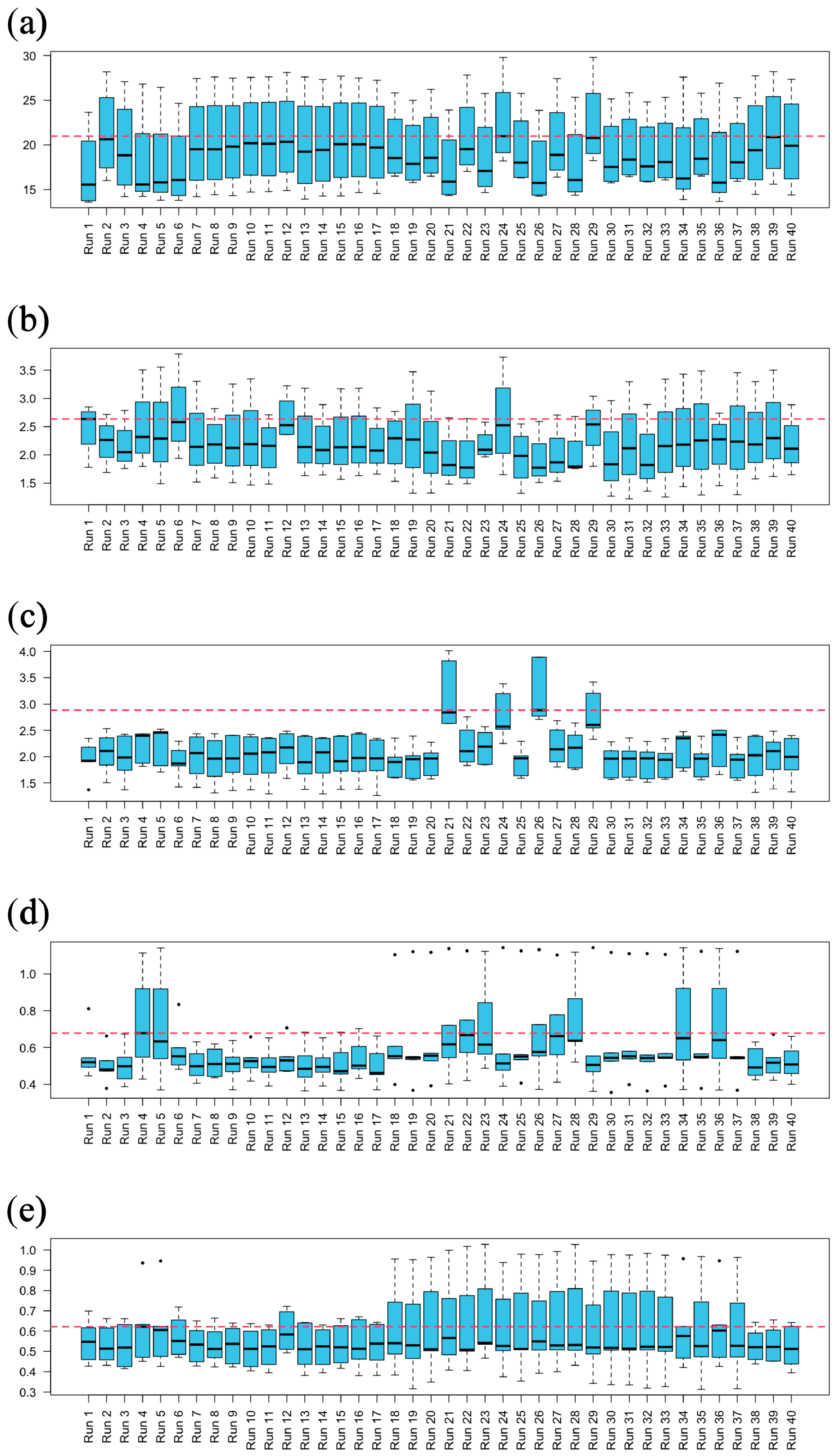
The FAC2 and RMSE distributions across the 40 runs are shown as box plots in Figure 2 and Figure 3, respectively. FAC2 was not computed for the absolute temperature because the factor-of-two criterion is not physically meaningful for this variable when expressed on an absolute temperature scale. Therefore, FAC2 was reported only for the remaining meteorological variables as a complementary diagnostic metric. For relative humidity, FAC2 was maximized by run 32 (highest median value). Analyzing the wind speed results, FAC2 showed that run 31 was the best option, with a slight difference from the other runs, considering the maximum median of the boxplots. In contrast, the results for Dir-x and Dir-y suggested configurations for runs 15 and 13, respectively.

The RMSE, which preserves the physical units of each variable and therefore cannot be compared across variables, nominated a third and again distinct set of configurations: run 1 for relative humidity, run 26 for temperature, run 6 for wind speed, and runs 17 and 22 for Dir-x and Dir-y, respectively. Thus, within the two scale-dependent metrics alone, the identity of the “best” run changed with essentially every variable.

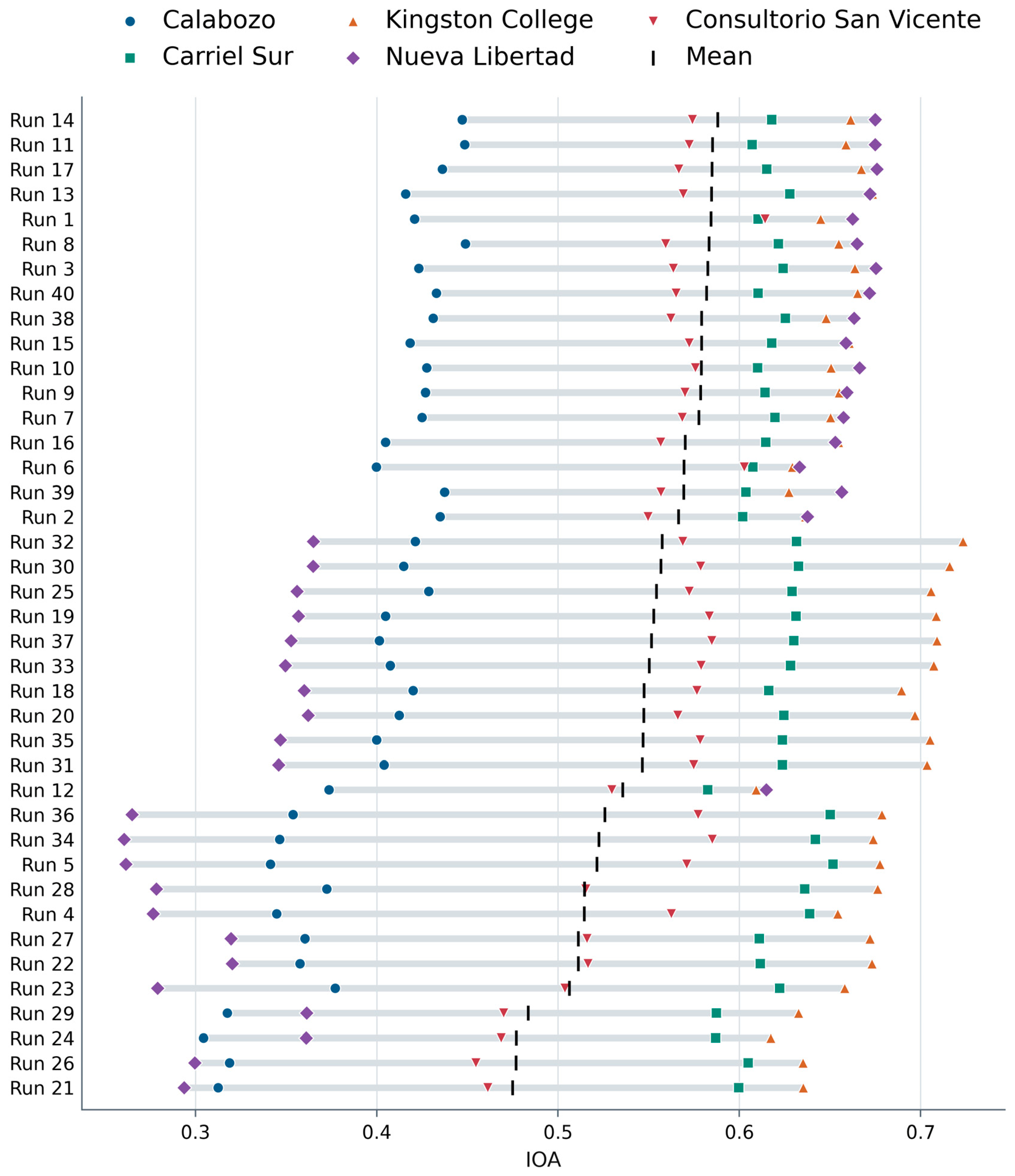
In the case of the IOA, this indicator is dimensionless; therefore, the values obtained for meteorological variables measured on different physical scales are directly comparable and can be averaged without additional scale standardization. Higher IOA values indicate better agreement between the simulated and observed values. Figure 4 shows the obtained values for the IOA metric for all stations and all meteorological variables studied. Additionally, the mean for each run is presented.

The IOA, being dimensionless and bounded in [0, 1], permits aggregation across variables, and the best configuration is the one that maximizes its value. The maximum mean IOA was attained by run 14 (0.588), narrowly ahead of runs 11, 17, 13, and 1 (0.584–0.585). Two features deserve emphasis. First, run 14 did not attain the maximum IOA for any individual variable at any individual station; its leading position is an artifact of averaging heterogeneous partial scores, which illustrates how fragile a simple mean of univariate indices can be. Second, the five leading IOA configurations all share the MM5 surface-layer scheme paired with the YSU PBL scheme—a family that, as shown next, the multivariate criterion does not favor.

Taken together, FAC2, RMSE, and IOA nominated at least eight different optimal runs (1, 6, 13, 14, 15, 17, 22, 26, 31, and 32) depending on the variable and metric consulted. This lack of a consistent, defensible ranking leaves the modeler without an objective basis for selecting a single configuration, with direct consequences for any subsequent pollutant-dispersion simulation that depends on the chosen meteorology. The results indicate that the use of traditional statistical indicators generates results with discrepancies between them, making it difficult to decide on the best meteorological simulation run, which could have a negative impact on the subsequent simulation of pollutant dispersion.

3.2. Mahalanobis Distance Results

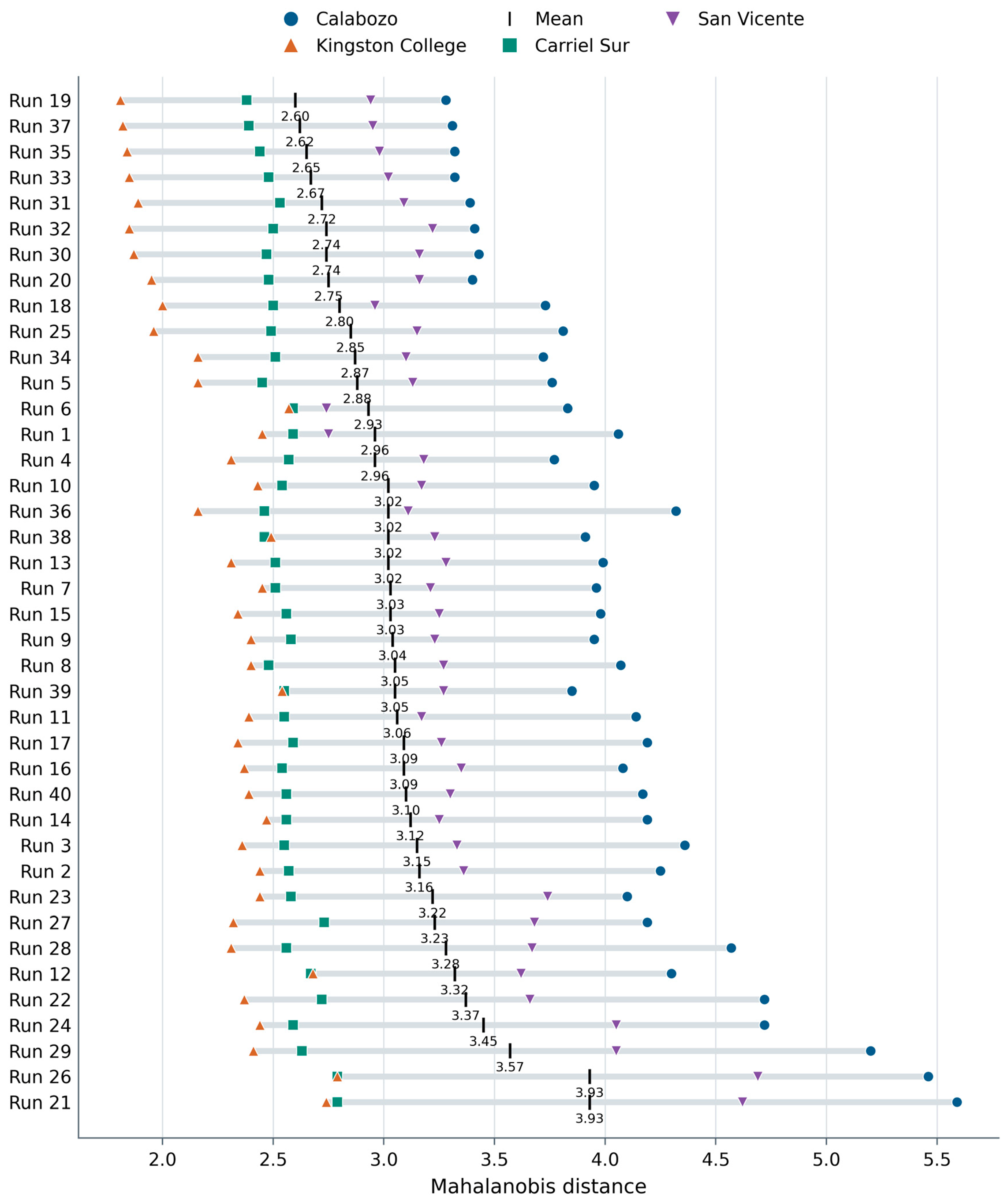
Figure 5 shows the aggregated Mahalanobis distance for each run at the four stations with complete variable coverage (San Vicente, Calabozo, Kingston College, and Carriel Sur), together with the cross-station mean; Nueva Libertad, which records only wind variables, was excluded from the multivariate computation because the metric requires the full set of jointly observed variables. The mean distances ranged from 2.60 to 3.93. Run 19 attained the minimum mean distance and, notably, the minimum per-station distance at three of the four stations (Calabozo 3.28, Kingston College 1.81, and Carriel Sur 2.38); at Consultorio San Vicente it ranked among the leading runs (2.94, versus a best of 2.74). In contrast to the fragmented univariate analysis, the multivariate criterion yields a single, spatially consistent recommendation.

The ranking exhibits a clear physical structure. The ten best runs by mean distance combined the GFS surface-layer scheme with the GFS PBL scheme, while differing freely in microphysics (Kessler, WSM3, and WSM6, Goddard), radiation (RRTM/Dudhia and CAM, RRTMG), and cumulus options. Conversely, the two worst runs (21 and 26; mean 3.93) used the QNSE surface layer/PBL pairing, and the BouLac PBL runs (24 and 29) were ranked near the bottom of the list. The spread attributable to the surface layer/PBL choice (≈1.3 distance units) was roughly an order of magnitude larger than the spread among microphysics or radiation options within the leading PBL family (≈0.1–0.2 units), indicating that these two schemes dominated the near-surface performance in this domain and season.

At the station level, the Calabozo station systematically exhibited the largest distances across all 40 configurations (3.28–5.59), indicating that no parameterization reproduces the joint behavior of the observed variables there as faithfully as at the other sites—a signal that points to a site-specific rather than a configuration-specific limitation. Finally, run 19 attained the lowest aggregated Mahalanobis distance among the 40 configurations, indicating the smallest joint multivariate discrepancy between the simulated and observed variables; lower values across configurations consistently identify the more faithful simulations, with run 19 being the closest to the observed multivariate behavior.

4. Discussion

4.1. The Mahalanobis Distance as a Unified Multivariate Decision Criterion

The central difficulty in parameterization selection is that the univariate performance depends on the target variable. For a fixed metric, the optimal configuration for temperature does not need to coincide with that for relative humidity or wind speed, and, as shown in Section 3.1, changing the metric changes the ranking again. In the present case, FAC2, RMSE, and IOA jointly nominated at least eight different “best” runs. The Mahalanobis distance resolves this fragmentation by construction rather than by post hoc averaging, because its three defining properties map directly onto the three failure modes observed for the univariate metrics. First, the implicit standardization by S⁻¹ removes measurement-scale effects, eliminating the artifact that rendered FAC2 uninformative for temperature and made RMSE incommensurable across variables with different units. Second, the use of the full inverse covariance matrix S⁻¹ accounts for inter-variable correlation, preventing double counting that affects any additive combination of univariate scores. Third, the aggregation in Equation (5) returns a single dimensionless scalar per station that can be averaged across stations sharing the same set of variables and compared across campaigns, models and regions.

Positioning the Mahalanobis distance alongside other comprehensive evaluation methods that have become popular in atmospheric science is enlightening. The Taylor diagram summarizes the correlation, standard deviation, and centered RMSE in a single plane and remains the most widely used tool. However, it assesses one variable at a time and does not, by itself, return a single scalar ranking; a recognized limitation is that it considers only a limited set of metrics and can therefore rank models inconsistently when several skill aspects matter [27].

DISO was proposed to convert the Taylor-diagram information into a single distance by merging the correlation coefficient, mean absolute error, and RMSE in a normalized space, and has since been applied widely to rank climate models and reanalyses and to evaluate physics modifications [11,12]. DISO and the Mahalanobis distance share the same underlying philosophy—collapse a model–observation comparison into one interpretable distance in which smaller is better—but operate on complementary axes. DISO integrates several statistics computed for a single variable, whereas the Mahalanobis distance integrates several variables while correcting for their covariance; the two are, in principle, composable, since a covariance-aware distance could be built over a vector of per-variable DISO scores.

Another relevant composite metric is the Kling–Gupta Efficiency (KGE), which is widely used in hydrological and climatic model evaluation because it combines correlation, bias, and variability into a single interpretable score [28]. However, in its standard formulation, KGE remains a univariate metric: it evaluates one simulated variable against one observed variable at a time. In the present application, KGE would therefore need to be computed separately for each meteorological variable and monitoring station, followed by an additional aggregation rule to obtain a single WRF configuration ranking. This would reintroduce the same decision problem that motivates the use of a multivariate criterion. In contrast, the Mahalanobis distance operates directly on the multivariate discrepancy vector and accounts for the covariance among variables.

Thus, Taylor diagrams, KGE, and DISO are valuable integrated or diagnostic tools, but they primarily summarize the performance attributes for individual variables and require an additional aggregation step when multiple variables and stations are jointly evaluated. The distinctive contribution of the Mahalanobis distance in this study is that it treats the error as a multivariate structure, accounting for inter-variable covariance and scale differences, and under approximate normality, attaches an absolute χ² reference to the resulting distance rather than a purely relative ordering.

4.2. Robustness, Assumptions, and Practical Guidance

The framework has identifiable costs and failure modes, which we state explicitly to guide adoption. First, estimating the covariance matrix S requires a record length n comfortably larger than the number of variables k; with the hourly series used here (n on the order of several hundred per station for k = 5), the estimate is stable, but for short campaigns, a regularized or shrinkage estimator should replace the sample covariance to keep S well conditioned. Second, the sample covariance is sensitive to outliers, and robust plug-in estimators, such as the minimum covariance determinant, are natural replacements; this both stabilizes the distance and connects the present framework to the extensive literature in which the Mahalanobis distance is used for multivariate outlier detection [10] and robust performance evaluation. Third, the metric weights variables according to their joint statistical variability rather than their importance for a given application; when a downstream use is dominated by one variable—wind for the dispersion of a buoyant plume, for instance—a weighted variant of Equation (1) can encode that priority without abandoning the covariance correction. Finally, the χ² threshold and Gaussian limit invoked in Equations (4)–(6) assume approximate normality of the difference series; for strongly skewed variables, a transformation or a bootstrap calibration of the threshold is advisable, and confirming the normality assumption is a sensible pre-processing step in any application.

This consideration becomes particularly relevant when extending the framework to additional meteorological variables. The present analysis was restricted to variables for which available and consistent station observations existed during the simulation period. The Mahalanobis distance framework can be expanded to include other meteorological variables, such as precipitation, cloudiness, or solar irradiance, by increasing the dimension of the multivariate vector. However, this extension is not purely mechanical, because these variables may involve missing data, intermittent behavior, bounded values, skewed distributions, or a larger covariance matrix that requires a sufficient sample size for stable estimation.

Similarly, air pollutants can be evaluated within the same statistical framework, but they should not be mixed directly with meteorological variables in a single Mahalanobis distance calculation, as they represent a distinct downstream response of the modeling system. Therefore, pollutant concentrations would be more appropriately analyzed in an independent multivariate framework.

4.3. Physical Interpretation and Transferability of the Demonstration

Beyond nominating a single configuration, multivariate ranking helps identify which of the physics options varied in this experiment most strongly influenced the near-surface performance in this coastal, topographically complex domain. The leading configurations differed widely in microphysics and radiation but coincided in the GFS surface-layer/GFS PBL pairing, and the ranking deteriorated sharply for the QNSE and BouLac families. Thus, within the parameterization families varied in this study, the surface-layer and boundary-layer schemes had a clearer influence on the multivariate ranking than the microphysics and radiation options included in the tested subset.

This hierarchy, among the parameterization families varied in this study, such as the boundary-layer and surface-layer schemes first, microphysics and radiation second, is physically reasonable for the evaluated variables and the late winter period, because near-surface temperature, humidity, and wind at hourly resolution are governed primarily by the representation of vertical mixing and surface exchange, whereas microphysics differences act mainly on precipitation processes that project only weakly onto these variables over the simulated window. However, this interpretation must be bounded by the experimental design. The land surface scheme was kept fixed across all simulations; therefore, the present study cannot quantify the uncertainty associated with land surface parameterization or its potential interaction with the surface layer and PBL schemes. Because the land surface scheme directly influences heat, moisture, and momentum fluxes, its fixed treatment represents an important limitation of the sensitivity experiment. Consequently, the present result should be interpreted as evidence of the importance of the surface layer/PBL pairing among the schemes varied here, rather than as a general statement that all near-surface parameterizations dominate model performance. Future studies should include multiple land surface schemes to explicitly evaluate this source of uncertainty.

The result is consistent with the broader finding that PBL and surface-layer parameterizations are leading sources of spread in WRF-simulated surface fields, although the specific scheme that performs best is strongly region-dependent: high-latitude and mid-latitude studies have recommended other pairings, such as the MYNN and YSU families, for surface wind and temperature [29]. This apparent disagreement is the point—no configuration is universally optimal, which is precisely why an objective, transferable selection criterion is needed rather than a fixed recommended scheme. We therefore read the present outcome as evidence that the GFS surface-layer/GFS PBL pairing best reproduces the joint variability of the observed surface variables among the configurations tested in this domain and season, not as a general endorsement of that family.

The divergence between the two integrated criteria applied in this study is noteworthy: the mean-IOA ranking preferred the MM5/YSU family (run 14), whereas the Mahalanobis distance favored the GFS/GFS family (run 19). This distinction is significant because these families employ different surface and boundary-layer schemes. The consistently large distances observed at Calabozo underscore the practical advantages of employing a per-station multivariate distance approach. A uniformly high value across all configurations suggests that the mismatch is structural, potentially due to unresolved local circulations at a 1 km resolution, siting effects, or observational issues, rather than being attributable to any single scheme.

4.4. Implications for Air Quality Modeling and Outlook

To the best of our knowledge, the Mahalanobis distance has not been previously used as a decision criterion for selecting physics parameterizations in meteorological simulations. Existing scheme-selection studies rely on univariate benchmarks, Taylor-type summaries, or feature-based scores, and the metric’s prior atmospheric use has been confined to multivariate outlier detection, for example, in particulate matter forecasting [18]. The relevance for air quality modeling is direct. Errors in wind speed and direction propagate into transport and plume impact; errors in temperature and humidity propagate into reaction rates, gas–particle partitioning, and biogenic emissions; and the boundary-layer representation controls the dilution volume available to primary pollutants. Because no single meteorological variable dominates all these pathways, a selection criterion for AQM-oriented meteorology should be inherently multivariate, which is the property of the Mahalanobis distance. A natural next step, beyond the scope of this study, is to propagate the competing configurations through a chemical transport model and verify whether the multivariate meteorological optimum minimizes errors in the simulated pollutant concentrations.

Subsequently, pollutant observations could be incorporated by constructing a separate pollutant-error vector from paired observed and simulated concentrations, for example, for PM_2.5, ozone (O₃), nitrogen dioxide (NO₂), or sulfur dioxide (SO₂). The MD could then be computed independently for this air-quality vector to assess whether the meteorological configuration selected from WRF also improves pollutant predictions. Pollutants should not be mixed directly with meteorological variables in the same WRF-only evaluation vector because their concentrations depend not only on meteorology but also on emissions, chemistry, deposition, and boundary conditions. Thus, pollutant-based MD should be interpreted as a downstream air-quality validation layer rather than as part of the present meteorological selection criterion.

Several limitations bound the demonstration and frame future work. The evaluation covers a single late-winter period over one region and four multivariate stations; the metric itself is season- and region-agnostic, but the specific ranking of configurations is not, so multi-season and multi-region replications are needed before a configuration is adopted operationally. Consistent with this, the MD identified a single configuration attaining the minimum distance at three of the four stations, indicating that genuine spatial heterogeneity in model performance can persist even after the multivariate correction; denser networks would help establish whether this reflects station-specific behavior or sampling noise, and a modeler facing this situation could adopt either a domain-averaged MD across stations or a station-specific configuration for critical individual sites, cross-validated to avoid overfitting.

The 40 configurations followed a sequential screening design rather than a full factorial, chosen for computational feasibility rather than as an inherent requirement of the method; the same MD-based decision framework applied regardless of whether the tested set comprised five, ten, or dozens of configurations. This design leaves scheme interactions outside the sampled combinations unexplored; therefore, we treat the surface-layer/PBL signal identified here as a prioritization hypothesis for a subsequent confirmatory factorial experiment, rather than as an operational recommendation in itself.

No observational nudging was applied, a deliberate choice to evaluate the free-running skill of each configuration, but one that leaves open how the ranking would change under data assimilation. Subject to these caveats, the results support the adoption of the Mahalanobis distance as the primary criterion whenever several meteorological variables at several stations must be evaluated jointly, with the traditional univariate metrics retained in a complementary, diagnostic role. The robust and weighted variants outlined above should be applied when the record is short or the application privileges particular variables.

5. Conclusions

When selecting a WRF configuration using a conventional univariate performance metric, the preferred configuration may depend on the target variable, monitoring station and metric considered. In this study, FAC2, RMSE, and IOA produced different rankings across meteorological variables and stations. These inconsistencies do not imply that traditional metrics are not useful; rather, they show that univariate indicators are better suited for diagnostic interpretation than for selecting a single configuration when several variables must be evaluated jointly.

The Mahalanobis distance provided a complementary multivariate criterion for this decision problem. Its main advantage is that it summarizes the joint discrepancy between simulations and observations while accounting for differences in the measurement scale and inter-variable correlation. Therefore, it allows meteorological variables of different natures, such as temperature, relative humidity, wind speed, and wind direction components, to be evaluated within a common statistical framework.

Among the 40 WRF physics configurations tested in this controlled sensitivity experiment, run 19 yielded the lowest mean Mahalanobis distance and the lowest station-specific distance at three of the four stations included in multivariate calculation. Therefore, run 19 should be interpreted as the best-performing configuration among the tested schemes, rather than a universally optimal configuration for the region. Among the tested configurations, those with lower Mahalanobis distance values were closer to the observed multivariate meteorological behavior, with run 19 attaining the smallest discrepancy.

The multivariate ranking also suggested that, within the parameterization families varied in this study, the surface-layer/PBL pairing had a clearer influence on the performance ranking than the microphysics and radiation options included in the tested subset. However, this interpretation is constrained by the experimental design. The land surface scheme was kept fixed across all simulations; consequently, the present study could not quantify the uncertainty associated with land surface parameterization or its potential interaction with the surface layer and PBL schemes. Thus, the results should not be interpreted as a general statement that all near-surface parameterizations dominate the model performance. Overall, the results support the use of the Mahalanobis distance as a reproducible multivariate decision criterion when several meteorological variables and monitoring stations are evaluated simultaneously.