Machine Learning-Based Hydrological Drought Prediction Integrating Teleconnections and Hydrological Memory in a Semi-Arid Basin, Algeria

Abstract

Hydrological drought forecasting in semi-arid basins is challenging due to the combined influence of meteorological forcing, large-scale atmospheric teleconnections, and basin memory processes, which are rarely jointly analysed within a leakage-free predictive framework. This study addresses this gap by evaluating gradient-boosted trees and neural forecasting models for one-month-ahead prediction of the Standardized Runoff Index (SRI) in two sub-basins of the Wadi Sahaouat Basin, Algeria. The models include gradient-boosted regression trees (GBRT), A-N-BEATS, A-N-HiTS, and TiDE, representing distinct forecasting architectures. Predictors consist of the Standardised Precipitation Index (SPI), seven teleconnection indices (NAO, AO, EAWR, SCAND, MEI, SOI, WeMO), and their one- to three-month lags. Two scenarios are tested: Scenario 1 uses SPI and teleconnection lags only, while Scenario 2 additionally includes lagged SRI values (SRI_lag1–3) to represent hydrological memory. A train-only Variance Inflation Factor (VIF > 10) procedure is applied to remove multicollinearity without data leakage. In Basin 1, SRI lags were excluded due to strong collinearity with SPI lags (r = 0.984), resulting in identical inputs for both scenarios. In Basin 2, SRI lags were retained to assess their predictive contribution. GBRT achieved the best overall performance across both basins and scenarios, with mean RMSE, NSE, and KGE values of 0.0682, 0.9907, and 0.8945, respectively. TiDE ranked second overall, with a mean RMSE of 0.1166, followed by A-N-HiTS in third place with a mean RMSE of 0.1203 and A-N-BEATS with the weakest overall performance, with a mean RMSE of 0.2159. These results indicate that gradient-boosted trees remain highly competitive with neural models for small monthly hydrological datasets and that the value of hydrological memory is basin-dependent and varies according to its independence from concurrent meteorological forcing.

1. Introduction

Drought is a complex and recurrent hydro-meteorological phenomenon characterized by a prolonged deficiency of precipitation that leads to significant reductions in water availability across atmospheric, terrestrial, and hydrological systems [1]. It manifests in multiple forms, including meteorological, agricultural, and hydrological droughts. Each form represents a different stage of water deficit and collectively they exert profound impacts on ecosystems, agriculture, and socio-economic systems [2,3]. In semi-arid regions, where climatic conditions are inherently variable and water resources are already limited, droughts occur more frequently and with greater severity [4]. The combined influence of erratic rainfall patterns, high evapotranspiration rates, and increasing climate variability has further intensified regional vulnerability, making accurate drought assessment and timely prediction a critical priority [5,6].

Traditionally, drought assessment has relied on standardized indices such as SPI, SPEI, and PDSI, along with classical statistical approaches, to quantify drought severity and duration. While these methods provide valuable insights into drought characterization, they are inherently limited in capturing the complex, nonlinear interactions among hydro-meteorological variables [7,8]. These limitations become more pronounced under changing climate conditions, where non-stationarity and the increasing frequency of extreme events challenge the reliability of conventional statistical frameworks [9]. Empirical evidence further highlights these constraints; for instance, Yang et al. (2020) reported that PDSI overestimates global drought-affected areas by approximately 10–20%, despite showing moderate to strong agreement (r ≈ 0.6–0.8) with climate model estimates, with notable regional inconsistencies [10]. Similarly, Jain et al. (2015) demonstrated that although indices such as SPI, EDI, and CZI exhibit strong inter-correlation (r ≈ 0.85–0.95), simpler approaches like rainfall departure fail to adequately represent drought severity, while SPI-12 effectively captures major drought events (e.g., 2002 and 2007) in the Ken River Basin [11]. These findings underscore the need for more robust and adaptive methodologies.

Building upon these advancements, recent years have witnessed a rapid shift toward machine learning (ML) techniques for hydro-meteorological drought assessment and forecasting, owing to their ability to model complex, nonlinear relationships [12,13,14]. Models such as Artificial Neural Networks (ANN), Fuzzy Logic, Coactive Neuro-Fuzzy Inference System (CANFIS), Support Vector Machines (SVM), Adaptive Neuro-Fuzzy Inference System (ANFIS), Random Forest (RF), and Extreme Learning Machines (ELM), along with hybrid and deep learning approaches, have demonstrated strong capabilities in capturing intricate interactions among climatic and hydrological variables. By integrating multi-source datasets including precipitation, temperature, evapotranspiration, soil moisture, and remote sensing variables, ML models significantly enhance drought prediction accuracy and robustness [15,16,17,18,19,20]. For instance, ANN achieved the highest prediction accuracy (NSE ≈ 0.92–0.96; RMSE ≈ 0.10–0.18), outperforming conventional approaches, while SVM and RF also exhibited strong performance (NSE ≈ 0.85–0.93). Further improvements were achieved using hybrid ELM models in the Wadi Mina Basin, with NSE values of approximately 0.95–0.98 and prediction errors reduced by 15–25% [21]. A GAM-based hybrid statistical–machine learning model for meteorological drought forecasting also demonstrated strong predictive performance, with NSE ≈ 0.88–0.94 and RMSE ≈ 0.10–0.20, outperforming traditional statistical models (NSE ≈ 0.75–0.85) and reducing forecast error by approximately 10–25% across different lead times [22]. More recently, Random Forest (RF), Support Vector Machine (SVM), Gradient Boosting Machine (GBM), and Artificial Neural Network (ANN) achieved high predictive accuracy for meteorological drought forecasting, with NSE ≈ 0.90–0.97, RMSE ≈ 0.08–0.18, and MAE ≈ 0.05–0.12, reducing prediction error by approximately 15–25% compared with conventional models in semi-arid regions [23].

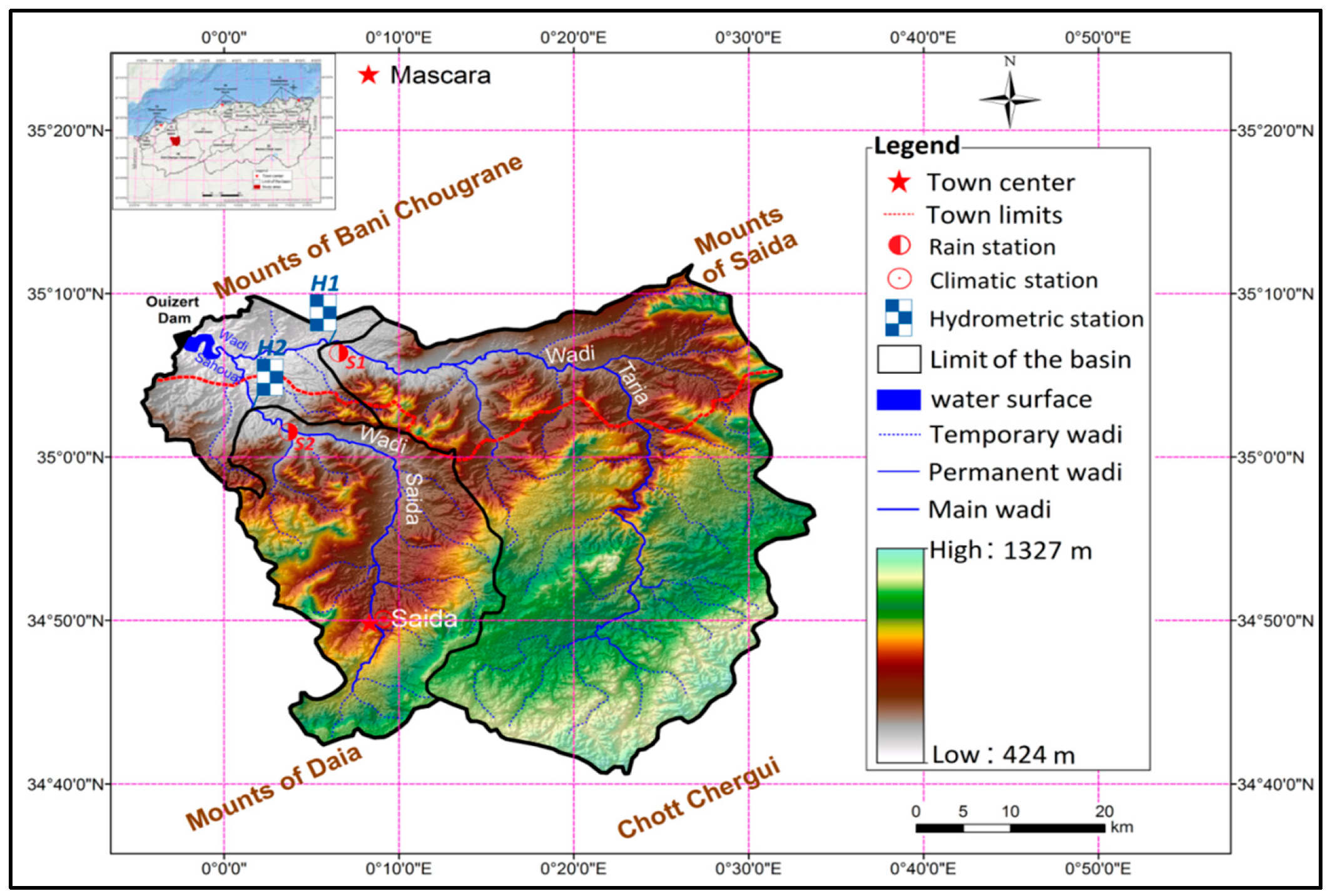
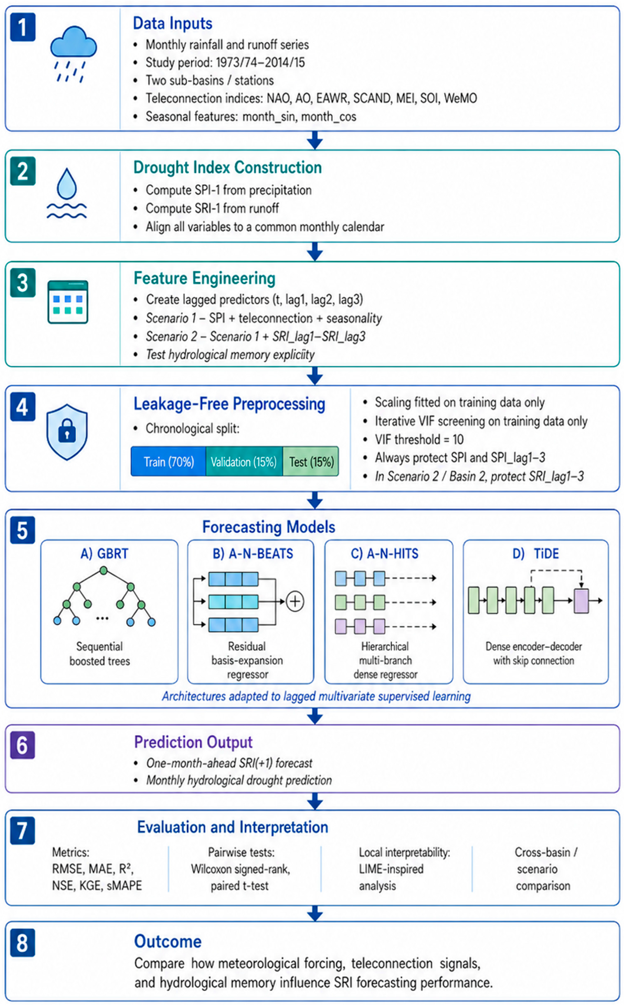
Despite these advancements, significant research gaps remain in integrating lagged multivariate inputs with emerging deep learning architectures for short-term hydrological drought prediction, particularly in data-scarce semi-arid basins. Moreover, limited attention has been given to disentangling the relative influence of atmospheric teleconnections, basin memory, and local meteorological drivers within unified modeling frameworks. The present study aims to develop a lagged multivariate forecasting framework for one-month-ahead prediction of the Standardized Runoff Index (SRI) in the semi-arid Wadi Sahaouat Basin (Algeria) by comparing the performance of gradient-boosted regression trees (GBRT) and advanced neural architectures (A-N-BEATS, A-N-HiTS, and TiDE), while disentangling the relative contributions of meteorological forcing, atmospheric teleconnections, and basin memory processes in hydrological drought prediction.

2. Data and Methodology

2.1. Study Area and Data

The Wadi Sahaouat basin (2140 km²) is a sub-basin of the Macta basin (14,390 km²), located approximately 400 km west of Algiers (Figure 1). The basin is bounded by longitudes 0°07′ E and 0°56′ E and latitudes 35°07′ N and 35°20′ N, and encompasses two main administrative provinces Saida (75% of the total area) and Mascara (25%). The Digital Elevation Model (DEM, 30 m resolution; downloaded from http://earthexplorer.usgs.gov/) indicates that the basin ranges in elevation from 424 m to 1327 m above sea level, with the highest-altitude class (1000–1200 m) covering 35.22% of the total area. The Wadi Sahaouat watercourse is formed by the confluence of Wadi Taria and Wadi Saida, with a total channel length of 98 km, supplying the Ouizert dam reservoir, which has an initial storage capacity of 100 hm³.

Monthly rainfall and runoff records were obtained from the National Agency for Hydraulic Resources (ANRH) as shown in

Table 1. Characteristics of the meteorological (S1–S2) and hydrological (H1–H2) stations used in the study. The table distinguishes the available station archive from the common monthly period used for modelling.

No.	Station Name	Station ID	Sub-Basin	Longitude (°)	Latitude (°)	Altitude (m)	Available Station Archive	Common Modelling Period
S1	Oued Taria	111201	Taria	0°5′42″ E	35°6′ N	498	1973/74–2014/15	January 1979–August 2015, n = 440
S2	Sidi Boubekeur	111102	Saida	0°3′38″ E	35°1′ N	525
H1	Oued Taria	111201	Taria	0°07′ E	35°10′ N	501
H2	Sidi Boubekeur	111129	Saida	0°02′ E	35°05′ N	540

. Although the available station archive extends over 1973/74–2014/15, the forecasting experiments were conducted using the common monthly period shared by the rainfall, runoff, teleconnection, SPI/SRI, and lagged predictor datasets. After temporal alignment and feature construction, the final modelling dataset covered 1979–2015, corresponding to 440 monthly records for each basin. All SPI-1 and SRI-1 calculations, lagged predictor construction, VIF screening, chronological train–validation–test splitting, and model evaluation were therefore performed on this common modelling period.

The climatology of the study area is typically Mediterranean continental. The analysis of the monthly temperatures (T) over 34 years (1977/2010) of the Saida station (ID: 536) showed that July and August are the hottest months of the year, with average temperatures of 27 °C, while January records low temperatures of up to 3.1 °C. The inter-annual average temperature is 16.7 °C. The mean annual relative humidity (RH) is 58%. Monthly RH exhibits a pronounced seasonal pattern, with the lowest values occurring in July (mean: 39%), when monthly averages can decrease to as low as 17% in some years. In contrast, the highest RH values are observed during the winter months (December–February), with monthly means ranging from 68% to 71% and reaching up to 90% in individual years. For the wind speed (Ws), Average monthly wind speeds generally range from 2.4 m/s in September and October to 3 m/s in April. Analysis of sunshine hours at the Saida station shows that the highest level was recorded in July, with an average of 325 h, and the lowest in January, with 183 h. Furthermore, the calculation of corrected potential evapotranspiration showed a maximum value of 139.70 mm and a minimum of 17.80 mm. Summer is the most dominant period of the year, due to the rise in temperature at this time of year. The aridity index, which stands at around 12.94 at the Saida station, reflects a semi-arid climate.

2.2. Drought Index Calculation

The quantitative assessment of drought in this study is conducted using a suite of standardized and multivariate indices, providing a multi-dimensional perspective on water deficits. To ensure computational consistency and transparency, all drought indices, including meteorological and hydrological, were calculated using the PyDRGHT Python 3.11.9 package [24].

2.2.1. Standardized Precipitation Index (SPI)

The Standardized Precipitation Index (SPI) (McKee et al. 1993) is the primary metric used to quantify meteorological drought by assessing precipitation deficits over user-defined timescales [25]. The calculation begins by fitting long-term monthly precipitation data to a probability density function, most commonly the Gamma distribution, given its effectiveness in representing skewed rainfall data [26]. The Gamma distribution is defined by the function:

$$\begin{array}{c}\mathrm{f}\left(\mathrm{x}\right)={\displaystyle \frac{1}{{\mathsf{\beta }}^{\mathsf{\alpha }}\mathsf{\Gamma }\left(\mathsf{\alpha }\right)}}{\mathrm{x}}^{\mathsf{\alpha }-1}{\mathrm{e}}^{-{\displaystyle \frac{\mathrm{x}}{\mathsf{\beta }}}}\end{array}$$

(1)

where α and β represent the shape and scale parameters, respectively, and Γ(α) is the Gamma function. Since precipitation data often includes zero values where the Gamma function is undefined, the cumulative probability H(x) is adjusted using the formula:

$$\begin{array}{c}\mathrm{H}\left(\mathrm{x}\right)=\mathrm{q}+\left(1-\mathrm{q}\right)\mathrm{G}\left(\mathrm{x}\right)\end{array}$$

(2)

where q is the probability of zero precipitation and G(x) is the cumulative probability from the fitted Gamma distribution. Finally, the cumulative probability is transformed into a standard normal variable (Z) with a mean of zero and a variance of one. This standardization allows the SPI to indicate the number of standard deviations an observed precipitation event deviates from the long-term median, with values below −1.0 generally indicating the start of a drought event.

2.2.2. Standardized Runoff Index (SRI)

The SRI serves as a critical indicator for hydrological drought, focusing on surface water availability rather than atmospheric moisture. The computational procedure for the SRI is mathematically analogous to the SPI; however, the input variable is streamflow or runoff data instead of precipitation. This index is particularly valuable because it incorporates hydrological processes such as snowmelt, infiltration, and groundwater lag, which often cause hydrological drought to persist even after meteorological conditions have improved. Runoff data is typically fitted to an appropriate distribution, such as the Log-normal or Gamma distribution, and then transformed into a standard normal distribution. The resulting index provides a standardized measure of water volume within the system, where negative values indicate a deficit in runoff relative to historical norms [27]. The SRI-1 timescale was selected to maintain consistency with the one-month-ahead forecasting framework adopted in this study. While longer timescales (e.g., SRI-3, SRI-6, and SRI-12) are commonly used to characterize seasonal and long-term hydrological drought conditions, the objective of this work was to evaluate short-term drought forecasting performance. Therefore, SRI-1 was considered the most appropriate indicator for the selected prediction horizon. Prior to standardization, runoff observations were examined for low-flow and zero-flow conditions to ensure the suitability of the fitted probability distribution. This procedure improves the reliability of the resulting SRI values and supports robust short-term drought assessment.

2.3. Predictor Design and Input Scenarios

2.3.1. Teleconnection and Seasonal Predictors

All analyses were conducted at the monthly time step. The core drought variables were SPI-1 and SRI-1, representing meteorological and hydrological drought at the same timescale. The teleconnection block comprised monthly series for the North Atlantic Oscillation (NAO), Arctic Oscillation (AO), East Atlantic/West Russia pattern (EAWR), Scandinavian pattern (SCAND), Multivariate ENSO Index version 2 (MEI), Southern Oscillation Index (SOI), and Western Mediterranean Oscillation (WeMO), aligned to a common monthly calendar. Although ENSO-related indices (MEI and SOI) are primarily associated with tropical Pacific variability, they are included due to their ability to influence North Atlantic and Mediterranean climate conditions through large-scale atmospheric teleconnection pathways and delayed circulation responses, which may indirectly modulate precipitation and drought dynamics in the study region. Seasonal structure was encoded through sine and cosine transformations of the calendar month (month_sin, month_cos), which preserve continuity between December and January and are better aligned with the physical periodicity of drought and teleconnection signals than a raw integer month label.

2.3.2. Lagged Predictors and Hydrological Memory

Lags were constructed deliberately rather than exhaustively. For every atmospheric index, the contemporaneous value and the one-, two-, and three-month lags were retained. The same lag depth was applied to SPI and, in Scenario 2, to SRI. This window is physically motivated: meteorological drought propagates into hydrological drought over timescales of weeks to a few months, depending on soil moisture buffering, catchment storage, and runoff response.

Multicollinearity was screened using the Variance Inflation Factor (VIF), computed exclusively on the training partition to prevent information from the validation or test sets from influencing feature selection. The procedure is iterative: at each step, the predictor with the highest VIF above a threshold of 10 is identified [28]; unless protected, it is removed and VIF is recomputed on the reduced set. SPI and its lags (SPI lag1–3) were always protected from removal as the primary meteorological forcing. In Scenario 2 for Basin 2, the lagged SRI values (SRI_lag1–3) were additionally protected to allow the scientific question of whether hydrological memory improves forecasting to be directly tested. Despite this protection, the VIF values of the SRI lags in Basin 2 were elevated (SRI_lag1 = 46.6, SRI_lag2 = 47.0, SRI_lag3 = 43.6), reflecting substantial but not perfect collinearity with SPI lags. In Basin 1, SRI lags were not protected because their VIF exceeded 40 (r = 0.984 collinearity with SPI lags), making their inclusion genuinely redundant. Despite its elevated VIF, SRI was intentionally retained because it represents hydrological memory and was needed to assess its added predictive value.

2.4. Leakage-Free Preprocessing

2.4.1. Chronological Train–Validation–Test Split

Model development followed a strictly chronological split: approximately 70% of the monthly series was assigned to training, the next 15% to validation, and the final 15% to testing. Predictor scaling was estimated from the training subset alone and applied to validation and test data. The same rule governed target scaling in the deep-learning models, ensuring that test scores reflect forward-looking model skill rather than leakage artefacts.

2.4.2. Scaling and VIF Screening

Two input scenarios were designed to isolate a specific hydrological question: is monthly streamflow deficit (SRI) primarily explained by concurrent and antecedent precipitation deficit (SPI) and atmospheric teleconnection forcing, or does the basin’s own recent hydrological history add predictive value beyond what meteorological signals provide?

Scenario 1 used SPI-1 (contemporaneous), SPI_lag1–3, seven atmospheric teleconnection indices and their lags 1–3, plus the two seasonal features, giving a maximum of 34 predictors before VIF screening. No SRI-derived predictor was included. Scenario 2 added SRI_lag1, SRI_lag2, and SRI_lag3, raising the maximum feature count to 37. Both scenarios used identical chronological splits and VIF screening logic; the sole structural difference was whether past SRI values were protected from removal and allowed to enter as predictors (

Table 2. Summary of the forecasting scenarios and corresponding predictor sets used for one-month-ahead SRI prediction. Scenario 2 includes lagged SRI variables in addition to the meteorological, teleconnection, and seasonal predictors considered in Scenario 1.

Scenario	Purpose	Predictors	Target
Scenario 1	Assess whether monthly meteorological drought and atmospheric forcing alone can explain hydrological drought.	NAO, AO, EAWR, SCAND, MEI, SOI, WeMO; lag1–lag3 for all teleconnections; SPI; SPI_lag1–lag3; month_sin; month_cos	SRI
Scenario 2	Assess whether adding lagged SRI values (hydrological memory) improves forecasting beyond Scenario 1.	All Scenario 1 predictors + SRI_lag1, SRI_lag2, SRI_lag3	SRI

).

Atmospheric oscillations influence hydrological drought through both direct meteorological forcing and delayed hydrological responses, as reflected in the variable design and lag structure used in this study. The inclusion of contemporaneous and 1–3 month lagged values of teleconnection indices (NAO, AO, EAWR, SCAND, MEI, SOI, and WeMO) indicates that their effects are not instantaneous but propagate over time. This is consistent with the physical understanding that meteorological drought, represented by SPI, translates into hydrological drought (SRI) over timescales of weeks to several months, depending on soil moisture storage, catchment characteristics, and runoff processes [29]. Previous studies have also shown that large-scale atmospheric circulation patterns significantly influence regional precipitation regimes and, consequently, streamflow variability [30,31]. In this study, results from Scenario 1 suggest that meteorological drought and atmospheric forcing alone can explain a substantial portion of hydrological drought variability, while Scenario 2 demonstrates that incorporating lagged SRI values improves predictions, highlighting the role of hydrological memory. This finding aligns with the understanding that hydrological systems are influenced not only by current atmospheric conditions but also by antecedent states [32,33].

The VIF procedure was used as a leakage-free screening tool, but physically meaningful predictors were allowed to be protected when they were required to test a specific hydrological hypothesis. In Scenario 2, SRI_lag1–3 were introduced to evaluate whether antecedent hydrological conditions add predictive information beyond SPI, teleconnection indices, and seasonality. Therefore, the final predictor sets were not forced to be identical across basins. In Basin 1, SRI lags were removed because they were nearly redundant with SPI lags, indicating that hydrological memory was not separable from meteorological memory at the monthly scale. In Basin 2, SRI_lag1–3 were retained as a controlled sensitivity experiment to quantify the predictive effect of hydrological memory despite high VIF values. Because the study is predictive rather than coefficient-explanatory, high VIF was interpreted as a caution for feature attribution, not as an automatic reason to remove hydrologically meaningful lag variables.

2.5. Forecasting Models

In this study, one tree-based benchmark and three custom neural forecasting variants were evaluated within a one-step-ahead lagged multivariate regression framework. The tree-based benchmark was implemented as GBRT (Gradient-Boosted Regression Trees), while the neural models were constructed as custom implementations inspired by N-BEATS (Neural Basis Expansion Analysis for Interpretable Time Series Forecasting), and N-HiTS (Neural Hierarchical Interpolation for Time Series Forecasting). Unlike their original sequence-based formulations, these architectures were applied to VIF-screened multivariate lagged predictors representing hydroclimatic memory, teleconnection signals, and seasonal covariates. Accordingly, the N-BEATS-inspired model was used as a residual fully connected forecasting block, the N-HiTS-inspired model as a multi-branch hierarchical dense regressor, and the TiDE-inspired model as a dense encoder–decoder regressor with a skip connection. Therefore, the present implementations should be interpreted as architecture-inspired neural regressors rather than exact replications of the original sequence-based forecasting models (Figure 2). For a one-month-ahead forecast, SRI(t + 1) was predicted exclusively from variables available at time t or earlier. No contemporaneous or future information from month (t + 1) was included among the predictors.

2.5.1. Gradient-Boosted Regression Trees (GBRT)

GBRT is a powerful ensemble learning method in which decision trees are trained sequentially, with each new tree learning the residual errors of the previous model to improve overall performance [34]. Due to its ability to capture nonlinear relationships, it is widely used in hydroclimatic forecasting problems [35].

In this study, the monthly lagged predictor set obtained after VIF screening was directly used as input to the GBRT model. Model performance was optimized through a compact hyperparameter search over the number of boosting rounds, learning rate, and tree complexity (max depth) on the validation set. These parameters are also central to modern gradient boosting frameworks [36].

2.5.2. Adapted Neural Basis Expansion Analysis for Time Series (A-N-BEATS)

The N-BEATS-inspired architecture offers a clear advantage through its residual, stacked fully connected structure, which progressively refines the predictive signal via successive nonlinear transformations. This design is well suited to capturing informative patterns in lagged hydroclimatic predictors while preserving a relatively simple and stable feed-forward formulation [37]. The model functions by iteratively decomposing the input into components that enhance both backcast and forecast representations. In this study, a custom NumPy-based implementation was developed in line with the original design principles and applied in a monthly forecasting context using the VIF-screened lagged predictor vector. N-BEATS was selected because drought dynamics often combine smooth, low-frequency variability with short-term anomalies, a structure that aligns naturally with residual basis expansion.

2.5.3. Adapted Neural Hierarchical Interpolation for Time Series (A-N-HiTS)

N-HiTS extends the N-BEATS framework by incorporating hierarchical interpolation and multi-rate processing. The N-HiTS-inspired model introduces a multi-branch architecture that enables the representation of predictor information at different levels of abstraction. This enhances predictive flexibility by allowing the model to capture both dominant patterns and finer-scale variations within lagged hydroclimatic inputs [38]. The architecture comprises three parallel branches operating at sub-sampling rates of 1, 2, and 3, each learning features at a distinct effective resolution before their outputs are combined. This configuration facilitates the separation of seasonal variability from inter-annual teleconnection signals, providing a physically meaningful inductive bias for modelling SPI-to-SRI propagation.

2.5.4. Time-Series Dense Encoder (TiDE)

TiDE is a dense encoder–decoder architecture designed to model multivariate covariates and nonlinear dependencies without relying on attention mechanisms [39]. The model encodes the input through multilayer perceptron blocks and decodes it into the forecast horizon, while a skip connection preserves the direct contribution of exogenous variables. TiDE was included because recent benchmarking studies indicate that carefully structured dense architectures can achieve strong performance when forecasting problems are governed by short memory and compact lag structures. Although N-BEATS, N-HiTS, and TiDE were originally developed as sequence-based forecasting models, they were implemented here as supervised regression models using lagged multivariate input features. As a result, the comparison reflects their behaviour within a tabular, feature-based forecasting framework rather than their original sequence-based formulations. Although the TiDE-based model was also implemented within the same forecasting framework, the original TiDE name was retained because the implemented structure follows the core TiDE formulation more directly. In contrast, the prefix “A-” was used for A-N-BEATS and A-N-HiTS to indicate more substantial architectural adaptations from the original N-BEATS and N-HiTS designs.

2.6. Local Interpretability

To support the physical interpretation of model outputs, a local surrogate explanation module was implemented following the LIME framework [40]. A LIME-inspired approach was applied to interpret the best-performing model at the instance level. For a selected input vector, 300 perturbed samples were generated, and model predictions were obtained for each sample. The distances between perturbed samples and the target instance were calculated, and a Gaussian kernel was used to assign proximity-based weights. A weighted Ridge regression model was then fitted locally, and the resulting coefficients were interpreted as local feature-importance scores (LIME weight), indicating both the direction and magnitude of each predictor’s contribution around the selected prediction.

2.7. Evaluation Metrics and Statistical Tests

Model performance was evaluated using RMSE, MAE, NSE, and KGE. RMSE and MAE quantify absolute forecast error, while NSE represents the proportion of explained variance. NSE and KGE provide hydrologically meaningful performance measures and are more interpretable than generic machine learning metrics when the target variable is a hydroclimatic index [41,42,43]. Statistical differences between model error distributions were assessed using the Wilcoxon signed-rank test and the paired-sample t-test, both applied to the 66-month held-out test set, which was not used during model training or hyperparameter tuning.

$$\mathrm{R}\mathrm{M}\mathrm{S}\mathrm{E}=\sqrt{{\displaystyle \frac{1}{\mathrm{n}}}{\sum }_{\mathrm{i}=1}^{\mathrm{n}}{\left({\mathrm{y}}_{\mathrm{i}}-{\hat{\mathrm{y}}}_{\mathrm{i}}\right)}^2}$$

(3)

$$\mathrm{M}\mathrm{A}\mathrm{E}=\left({\displaystyle \frac{1}{\mathrm{n}}}\right){\sum }_{\mathrm{i}=1}^{\mathrm{n}}\left|{\mathrm{y}}_{\mathrm{i}}-{\hat{\mathrm{y}}}_{\mathrm{i}}\right|$$

(4)

$$\mathrm{N}\mathrm{S}\mathrm{E}=1-\left[{\displaystyle \frac{{\sum }_{\mathrm{i}=1}^{\mathrm{n}}{\left({\mathrm{y}}_{\mathrm{i}}-{\hat{\mathrm{y}}}_{\mathrm{i}}\right)}^2}{{\sum }_{\mathrm{i}=1}^{\mathrm{n}}{\left({\mathrm{y}}_{\mathrm{i}}-{\stackrel{-}{\mathrm{y}}}_{\mathrm{i}}\right)}^2}}\right]$$

(5)

$$\mathrm{K}\mathrm{G}\mathrm{E}=1-\sqrt{{\left(\mathrm{r}-1\right)}^2+{\left(\mathsf{\alpha }-1\right)}^2+{\left(\mathsf{\beta }-1\right)}^2}$$

(6)

$$\mathsf{\alpha }={\displaystyle \frac{\mathsf{\sigma }\hat{\mathrm{y}}}{\mathsf{\sigma }\mathrm{y}}},\mathsf{\beta }={\displaystyle \frac{\mathsf{\mu }\hat{\mathrm{y}}}{\mathsf{\mu }\mathrm{y}}}$$

(7)

Here, y_i represents the observed value, ŷ_i is the predicted value, and ȳ is the mean of the observed values, while n denotes the number of observations. In the KGE metric, r is the correlation between observed and predicted values, α is the ratio of standard deviations and β is the ratio of means. Note that because SRI is a standardized, zero-centred index, the KGE bias-ratio component $\beta ={\mu }_{\widehat{y}}/{\mu }_y$ may become unstable when the observed mean over the test period is close to zero. Therefore, KGE was interpreted together with its components r, α, and β rather than as a standalone performance score.

3. Results

3.1. Basin 1: Forecast Performance

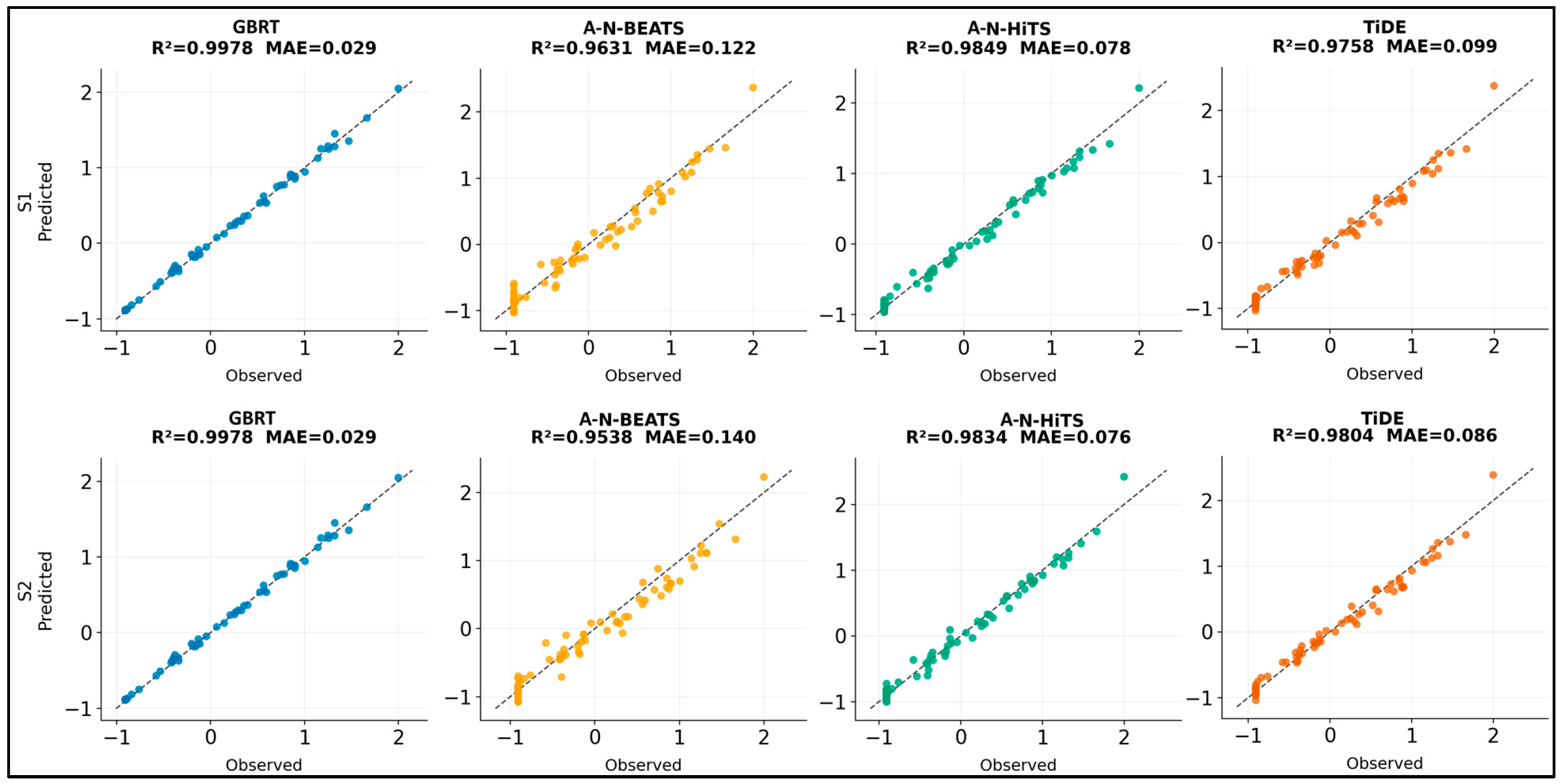
The GBRT model shows the strongest alignment, with NSE values around 0.997–0.998 and a low MAE of approximately 0.029. The points are tightly clustered along the diagonal, indicating that this model reproduces the observed values with relatively small deviations. Based on these findings, GBRT appears to provide the most consistent fit among the models shown.

The A-N-BEATS model demonstrates a slightly weaker performance, with NSE values around 0.95–0.96 and MAE values between 0.12 and 0.14. Although the general trend is still captured, the scatter around the diagonal is more pronounced, suggesting higher variability in the predictions compared to GBRT.

The A-N-HiTS model performs better than A-N-BEATS, with NSE values close to 0.98 and MAE around 0.076–0.078. The points are more tightly distributed along the diagonal, indicating improved predictive accuracy, though still not reaching the level observed in GBRT.

Finally, the TiDE model shows performance comparable to A-N-HiTS, with NSE values around 0.975–0.98 and MAE values ranging from approximately 0.086 to 0.099 (Figure 3). The predictions generally follow the observed values closely, although minor deviations are visible.

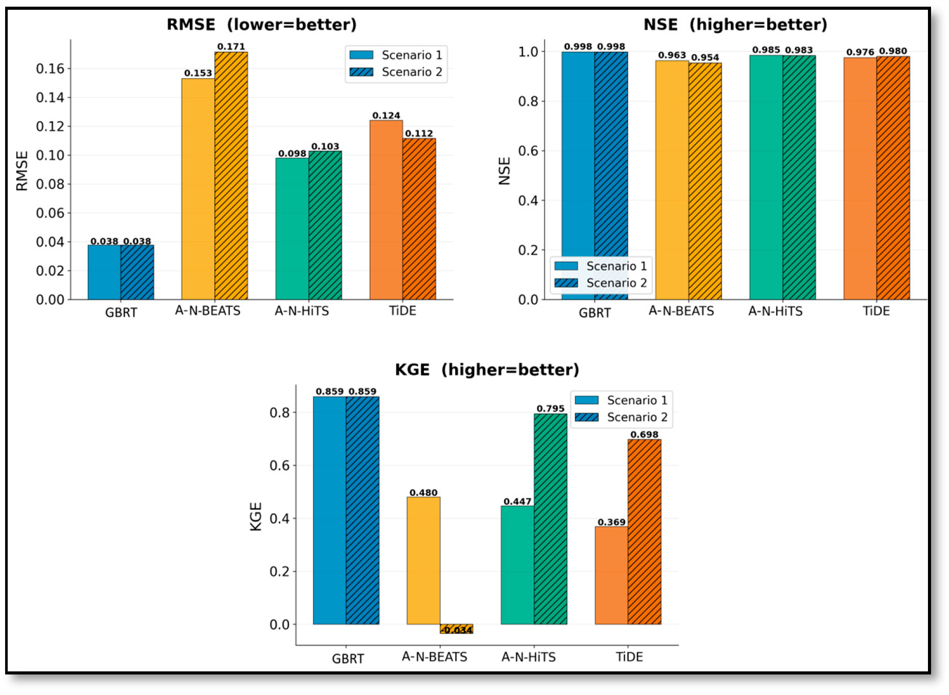
All metrics are computed on the 66-month held-out test set, which was withheld from both training and hyperparameter optimisation. In Scenario 1, GBRT achieved the best performance (RMSE = 0.0377, MAE = 0.0288, NSE = 0.9978, NSE = 0.9978, KGE = 0.8588). N-HiTS ranked second (RMSE = 0.0979, NSE = 0.9849, KGE = 0.4470), followed by TiDE (RMSE = 0.1240, KGE = 0.3695) and A-N-BEATS (RMSE = 0.1531, KGE = 0.4801).

In Scenario 2, VIF screening eliminated all three SRI lags owing to r = 0.984 collinearity with SPI lags; GBRT was therefore trained on an identical feature set and produced identical predictions (RMSE = 0.0377). Among the neural models, N-HiTS slightly worsened to RMSE = 0.1027 (KGE = 0.7948) and TiDE improved to RMSE = 0.1116 (KGE = 0.6976). A-N-BEATS deteriorated substantially (KGE = −0.0338), suggesting that its residual decomposition was destabilised by the autoregressive SPI lag configuration in this basin (

Table 3. Test-set performance metrics and ranking of the forecasting models in Basin 1 under both experimental scenarios.

Scenario	Model	RMSE	MAE	NSE	KGE	Features	Rank
Scenario 1	GBRT	0.0377	0.0288	0.9978	0.8588	32	1
Scenario 1	A-N-HiTS	0.0979	0.0780	0.9849	0.4470	32	2
Scenario 1	TiDE	0.1240	0.0989	0.9758	0.3695	32	3
Scenario 1	A-N-BEATS	0.1531	0.1225	0.9631	0.4801	32	4
Scenario 2	GBRT	0.0377	0.0288	0.9978	0.8588	32	1
Scenario 2	A-N-HiTS	0.1027	0.0757	0.9834	0.7948	32	2
Scenario 2	TiDE	0.1116	0.0864	0.9804	0.6976	32	3
Scenario 2	A-N-BEATS	0.1713	0.1404	0.9538	−0.0338	32	4

).

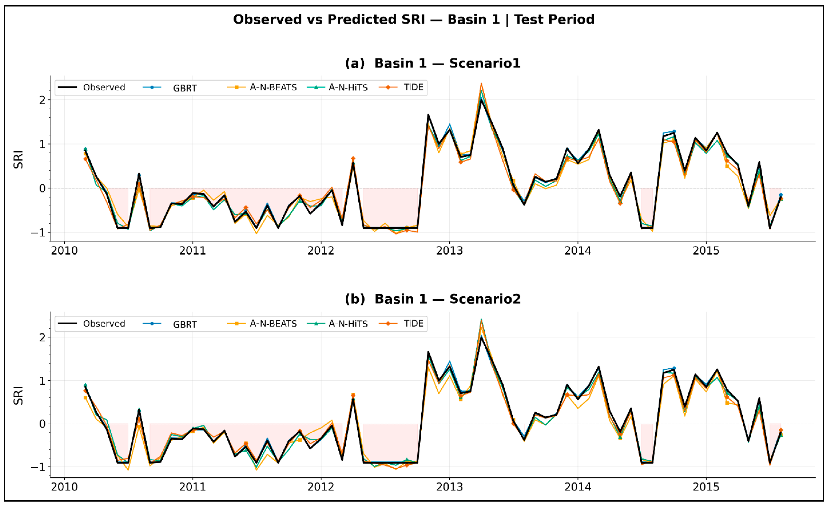
GBRT appears to align more closely with the observed values, showing smaller deviations during both low and high SRI conditions (Figure 4). A-N-HITS and TIDE also reproduce the general variability reasonably well, although some discrepancies are visible at peak events. A-N-BEATS shows comparatively larger deviations, particularly during sudden changes, which may suggest some limitations in capturing abrupt fluctuations.

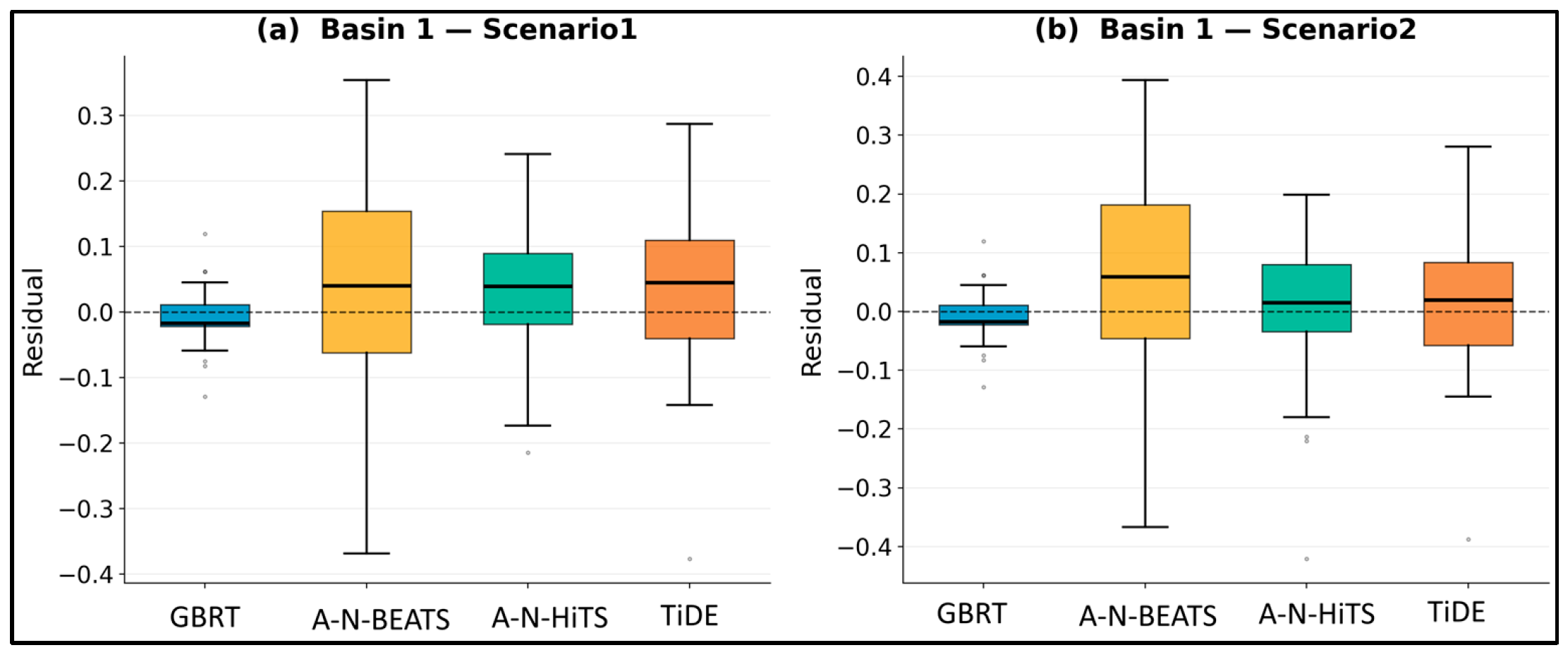
Residual boxplots further illustrate differences in model performance across Basin 1 scenarios (Figure 5). GBRT exhibits the narrowest residual distributions and medians closest to zero, indicating more accurate and stable predictions. A-N-HiTS and TiDE show relatively moderate residual variability, while A-N-BEATS displays the widest spread of residuals and the largest interquartile ranges, suggesting less consistent predictive performance. Although all models produce residuals on both sides of zero, the smaller dispersion observed for GBRT indicates lower prediction errors and greater robustness across the evaluated scenarios.

Residual boxplots and performance metrics provide a quantitative comparison. The residual distributions show that GBRT has a narrower spread centered near zero, which may indicate more stable and less biased predictions (Figure 6). A-N-BEATS displays a wider range of residuals, including more extreme values, implying higher variability. A-N-HiTS and TiDE fall between these two, with moderate dispersion.

The metric plots in Figure 6 support these observations. GBRT consistently achieves the lowest RMSE, along with the highest NSE and KGE values across both scenarios, indicating a closer match to observed data. A-N-HiTS and TiDE demonstrate intermediate performance, with moderate error levels and relatively strong efficiency scores. A-N-BEATS shows higher RMSE and lower NSE and KGE, suggesting comparatively larger deviations from observations.

All models capture the general behavior of SRI-1, but differences in accuracy and error distribution are evident, with GBRT showing more consistent agreement across the presented evaluations.

3.2. Basin 2: Forecast Performance

Basin 2 was analysed using its own SPI-1 and SRI-1 series over the common modelling period January 1979–August 2015, comprising 440 monthly records after temporal alignment and lagged predictor construction. In Scenario 1, GBRT ranked first (RMSE = 0.0985, NSE = 0.9837, KGE = 0.9286). TiDE ranked second (RMSE = 0.1258, KGE = 0.9372), A-N-HiTS third (RMSE = 0.1379, KGE = 0.8980), and A-N-BEATS fourth (RMSE = 0.2918, KGE = 0.8205).

In Scenario 2, SRI_lag1–3 were explicitly retained despite high VIF values (SRI_lag1 = 46.6, SRI_lag2 = 47.0, SRI_lag3 = 43.6). GBRT performance was essentially unchanged (RMSE = 0.0988, KGE = 0.9318), confirming that gradient-boosted trees already exploit the SPI-SRI relationship efficiently. TiDE improved substantially to RMSE = 0.1049 (KGE = 0.9878), the highest KGE recorded across all models and configurations; its encoder–decoder architecture with skip connections appears particularly effective at integrating autoregressive SRI signals with atmospheric covariates. A-N-HiTS achieved RMSE = 0.1428 (KGE = 0.9009). A-N-BEATS improved markedly from Scenario 1 (KGE = 0.8205) to Scenario 2 (KGE = 0.9453), indicating that its residual decomposition blocks can exploit SRI memory even when the direct meteorological signal is the dominant forcing (

Table 4. Test-set forecasting performance of the four models in Basin 2 under Scenario 1 and Scenario 2.

Scenario	Model	RMSE	MAE	NSE	KGE	Features	Rank
Scenario 1	GBRT	0.0985	0.0637	0.9837	0.9286	32	1
Scenario 1	TiDE	0.1258	0.1030	0.9734	0.9372	32	2
Scenario 1	A-N-HiTS	0.1379	0.1152	0.9680	0.8980	32	3
Scenario 1	A-N-BEATS	0.2918	0.2362	0.8568	0.8205	32	4
Scenario 2	GBRT	0.0988	0.0628	0.9836	0.9318	35	1
Scenario 2	TiDE	0.1049	0.0881	0.9815	0.9878	35	2
Scenario 2	A-N-HiTS	0.1428	0.1145	0.9657	0.9009	35	3
Scenario 2	A-N-BEATS	0.2473	0.2029	0.8972	0.9453	35	4

).

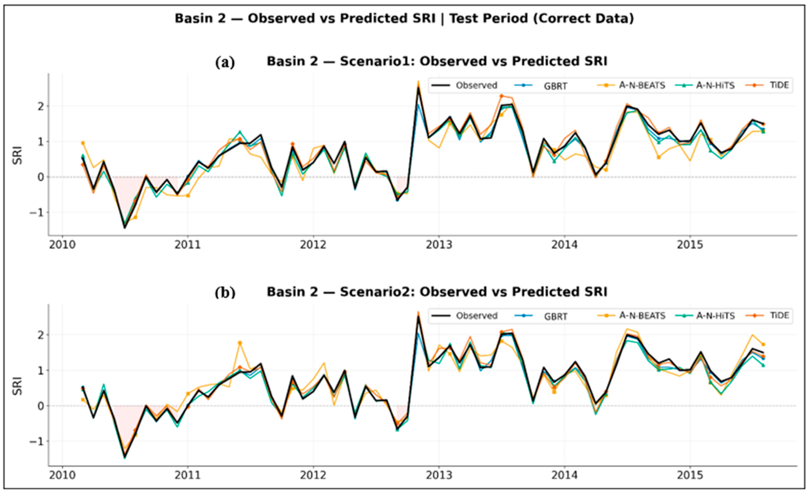
GBRT appears to track the observed series more closely, with relatively small deviations across the test period (Figure 7). A-N-HiTS and TIDE also capture the overall dynamics, although some differences are visible at peak values. A-N-BEATS shows comparatively larger departures, particularly during rapid changes, suggesting some difficulty in representing sharp transitions.

In Figure 8, Scenario 2 includes lagged predictors (SRI_lag1–3), a slight improvement in alignment can be observed for most models. The predictions appear somewhat smoother and closer to the observed series, especially for A-N-HiTS and TIDE. A-N-BEATS still exhibits noticeable deviations, although there is some reduction in extreme mismatches compared to Scenario 1.

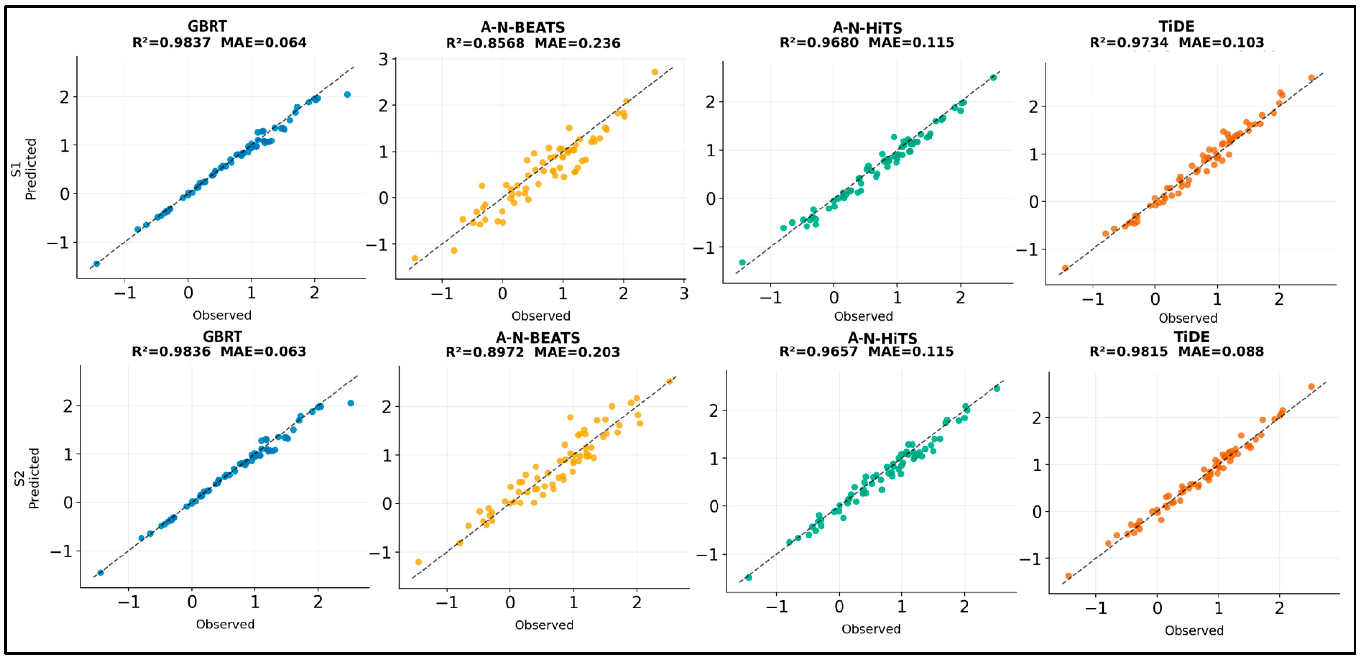
GBRT shows points tightly clustered around the 1:1 line, indicating strong agreement between observed and predicted values (Figure 9). A-N-HiTS and TiDE also demonstrate relatively good alignment, though with more dispersion than GBRT. A-N-BEATS displays a wider spread of points, which suggests higher variability and larger prediction errors. Points above and below the line indicate that both overestimation and underestimation occur across models, but these deviations appear more pronounced for A-N-BEATS.

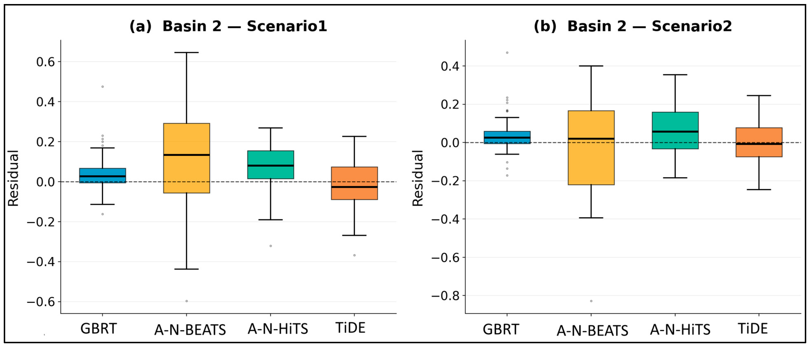
The residual distributions indicate that GBRT has a relatively narrow spread centered near zero, suggesting more stable predictions (Figure 10). A-N-BEATS shows the widest spread, including more extreme residuals, indicating higher variability. A-N-HiTS and TiDE fall in between, with moderate dispersion.

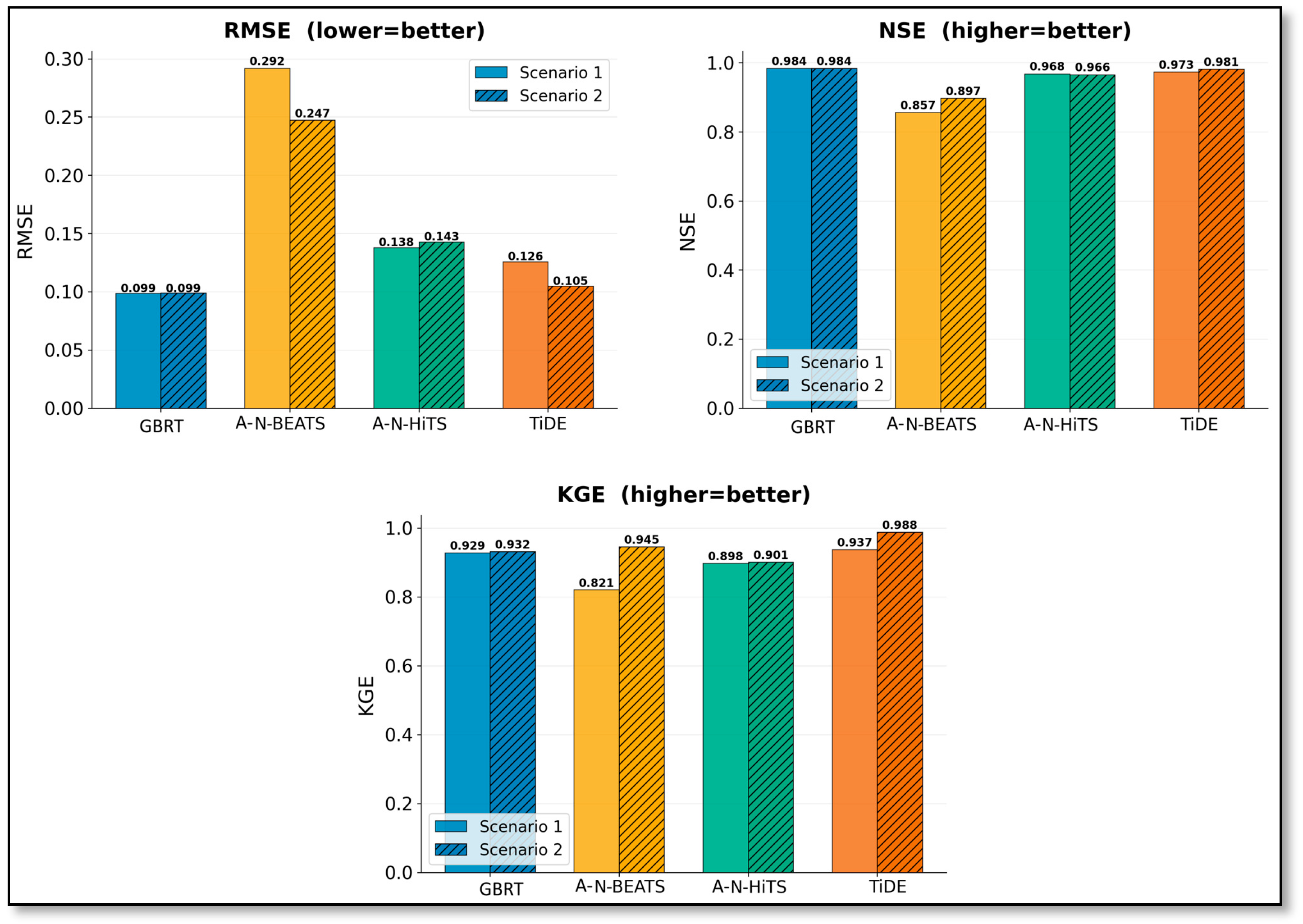
The metric comparisons are consistent with these observations. GBRT achieves the lowest RMSE (0.099), along with high NSE (0.984) and KGE (0.93) values across both scenarios. A-N-HITS and TiDE demonstrate intermediate performance, with moderate error levels and relatively high efficiency scores, and some improvement is visible in Scenario 2. A-N-BEATS shows higher RMSE (up to 0.292), along with comparatively lower NSE and more variable KGE values. All models capture the general behavior of SRI-1 in Basin 2, but their accuracy and consistency differ. GBRT appears to provide a more stable and closer agreement with observations, while A-N-HiTS and TIDE show moderate performance. A-N-BEATS exhibits higher variability and larger deviations, although some improvements are observed when lagged predictors are included in Scenario 2 (Table 5).

The marginal contribution of SRI_lag1–3 was evaluated by comparing Scenario 2 against Scenario 1 on the same held-out test period. In Basin 1, this contribution could not be separately estimated because VIF screening removed the SRI lags, producing effectively the same final input structure. This indicates that, in Basin 1, the antecedent runoff deficit largely overlaps with antecedent precipitation deficit. In Basin 2, however, retaining SRI_lag1–3 revealed a model-dependent hydrological-memory effect. TiDE improved from RMSE = 0.1258 to 0.1049 and KGE = 0.9372 to 0.9878, while A-N-BEATS improved from RMSE = 0.2918 to 0.2473 and KGE = 0.8205 to 0.9453. In contrast, GBRT remained essentially unchanged, suggesting that the tree-based model already exploited the SPI–SRI relationship efficiently. These findings indicate that hydrological memory provides additional predictive value in Basin 2, but the magnitude of this value depends on model architecture and on the degree to which SRI lags contain information not already represented by SPI lags.

For Basin 1, because SRI_lag1–3 was removed by VIF screening, the marginal contribution of SRI lags is not separately estimable. This result is itself hydrologically meaningful: in Basin 1, antecedent meteorological drought and antecedent hydrological drought are almost indistinguishable at the monthly scale.

For Basin 2, the marginal contribution of SRI_lag1–3 was quantified as follows:

Table 5. Comparison of model performance between Scenario 1 and Scenario 2 in Basin 2 and the associated changes in RMSE and KGE.

Model	RMSE Scenario 1	RMSE Scenario 2	ΔRMSE	KGE Scenario 1	KGE Scenario 2	ΔKGE	Interpretation
GBRT	0.0985	0.0988	+0.0003	0.9286	0.9318	+0.0032	Almost no marginal gain; GBRT already captures the SPI–SRI relation efficiently.
TiDE	0.1258	0.1049	−0.0209	0.9372	0.9878	+0.0506	Clear benefit from SRI memory; RMSE decreased by approximately 16.6%.
A-N-HiTS	0.1379	0.1428	+0.0049	0.8980	0.9009	+0.0029	No meaningful RMSE improvement; KGE changed only slightly.
A-N-BEATS	0.2918	0.2473	−0.0445	0.8205	0.9453	+0.1248	Strong improvement, although the model remains less accurate than GBRT and TiDE.

Table 5. Comparison of model performance between Scenario 1 and Scenario 2 in Basin 2 and the associated changes in RMSE and KGE.

Model	RMSE Scenario 1	RMSE Scenario 2	ΔRMSE	KGE Scenario 1	KGE Scenario 2	ΔKGE	Interpretation
GBRT	0.0985	0.0988	+0.0003	0.9286	0.9318	+0.0032	Almost no marginal gain; GBRT already captures the SPI–SRI relation efficiently.
TiDE	0.1258	0.1049	−0.0209	0.9372	0.9878	+0.0506	Clear benefit from SRI memory; RMSE decreased by approximately 16.6%.
A-N-HiTS	0.1379	0.1428	+0.0049	0.8980	0.9009	+0.0029	No meaningful RMSE improvement; KGE changed only slightly.
A-N-BEATS	0.2918	0.2473	−0.0445	0.8205	0.9453	+0.1248	Strong improvement, although the model remains less accurate than GBRT and TiDE.

These results show that the contribution of SRI_lag1–3 is model-dependent. It is small for GBRT, substantial for TiDE and A-N-BEATS, and limited for A-N-HiTS. Therefore, the inclusion of SRI_lag1–3 does not uniformly improve all models, but it reveals that some architectures are more sensitive to autoregressive hydrological memory than others.

3.3. Cross-Basin Model Ranking

Averaging performance metrics across both basins and both scenarios, GBRT ranked first overall (mean RMSE = 0.0682, NSE = 0.9907, KGE = 0.8945). TiDE ranked second (mean RMSE = 0.1166, NSE = 0.9778, KGE = 0.7480), A-N-HiTS third (mean RMSE = 0.1203, NSE = 0.9755, KGE = 0.7602), and A-N-BEATS fourth (mean RMSE = 0.2159, NSE = 0.9177, KGE = 0.5530). TiDE and A-N-HiTS were closely matched on average RMSE and NSE, but TiDE achieved the highest single-configuration KGE of any model (0.9878 in Basin 2, Scenario 2), consistent with its architecture benefiting most when SRI memory is available as a predictor (

Table 6. Overall performance ranking of GBRT, A-N-BEATS, A-N-HiTS, and TiDE based on average evaluation metrics computed across Basin 1, Basin 2, and both forecasting scenarios.

Rank	Model	Mean RMSE	Mean MAE	Mean NSE	Mean KGE
1	GBRT	0.0682	0.0460	0.9907	0.8945
2	TiDE	0.1166	0.0941	0.9778	0.7480
3	A-N-HiTS	0.1203	0.0959	0.9755	0.7602
4	A-N-BEATS	0.2159	0.1755	0.9177	0.5530

).

3.4. Statistical Significance and Local Interpretability

Pairwise differences in model forecast errors were examined using the Wilcoxon signed-rank test and the paired-sample t-test (

Table 7. Exploratory pairwise comparison of forecasting model errors in Basin 1 using the Wilcoxon signed-rank test and paired t-test. The reported p-values are unadjusted and should be interpreted cautiously because monthly residuals may exhibit serial dependence.

Scenario	Model A	Model B	W Stat	W p-Value	t Stat	t p-Value	Sig. (W)	Sig. (t)
Sc. 1	GBRT	A-N-BEATS	145	8.48 × 10−10	−7.754	8.00 × 10−11	Yes	Yes
Sc. 1	GBRT	A-N-HiTS	244	3.73 × 10−8	−6.032	8.52 × 10−8	Yes	Yes
Sc. 1	GBRT	TiDE	154	1.21 × 10−9	−7.402	3.37 × 10−10	Yes	Yes
Sc. 1	A-N-BEATS	A-N-HiTS	499	1.07 × 10−4	4.096	1.19 × 10−4	Yes	Yes
Sc. 1	A-N-BEATS	TiDE	851	0.104	2.136	0.036	No	Yes
Sc. 1	A-N-HiTS	TiDE	737	0.019	−2.215	0.030	Yes	Yes
Sc. 2	GBRT	A-N-BEATS	74	4.42 × 10−11	−9.123	3.01 × 10−13	Yes	Yes
Sc. 2	GBRT	A-N-HiTS	349	1.35 × 10−6	−5.184	2.31 × 10−6	Yes	Yes
Sc. 2	GBRT	TiDE	247	4.15 × 10−8	−6.319	2.72 × 10−8	Yes	Yes
Sc. 2	A-N-BEATS	A-N-HiTS	374	2.97 × 10−6	4.950	5.55 × 10−6	Yes	Yes
Sc. 2	A-N-BEATS	TiDE	464	4.17 × 10−5	4.868	7.54 × 10−6	Yes	Yes
Sc. 2	A-N-HiTS	TiDE	905	0.200	−1.123	0.266	No	No

Note: Significance at alpha = 0.05 is denoted “Yes”.

and

Table 8. Exploratory pairwise comparison of forecasting model errors in Basin 2 using the Wilcoxon signed-rank test and paired t-test. The reported p-values are unadjusted and are used only as supplementary diagnostics.

Scenario	Model A	Model B	W Stat	W p-Value	t Stat	t p-Value	Sig. (W)	Sig. (t)
Sc. 1	GBRT	A-N-BEATS	141	7.21 × 10−10	−7.798	6.66 × 10−11	Yes	Yes
Sc. 1	GBRT	A-N-HiTS	436	1.90 × 10−5	−3.865	2.59 × 10−4	Yes	Yes
Sc. 1	GBRT	TiDE	520	1.84 × 10−4	−3.229	1.95 × 10−3	Yes	Yes
Sc. 1	A-N-BEATS	A-N-HiTS	423	1.30 × 10−5	5.302	1.47 × 10−6	Yes	Yes
Sc. 1	A-N-BEATS	TiDE	271	9.78 × 10−8	6.112	6.20 × 10−8	Yes	Yes
Sc. 1	A-N-HiTS	TiDE	937	0.282	0.916	0.363	No	No
Sc. 2	GBRT	A-N-BEATS	189	4.78 × 10−9	−6.798	3.93 × 10−9	Yes	Yes
Sc. 2	GBRT	A-N-HiTS	392	5.17 × 10−6	−4.148	9.92 × 10−5	Yes	Yes
Sc. 2	GBRT	TiDE	672	5.62 × 10−3	−2.255	0.028	Yes	Yes
Sc. 2	A-N-BEATS	A-N-HiTS	497	1.01 × 10−4	4.354	4.84 × 10−5	Yes	Yes
Sc. 2	A-N-BEATS	TiDE	261	6.86 × 10−8	6.454	1.58 × 10−8	Yes	Yes
Sc. 2	A-N-HiTS	TiDE	783	0.039	2.244	0.028	Yes	Yes

). These tests provide exploratory information on whether the error distributions differ between model pairs. However, because the test data consist of monthly SRI forecasts, the resulting residuals and loss differences may not be fully independent. Therefore, the reported p-values should be interpreted cautiously and should not be treated as standalone proof of model superiority.

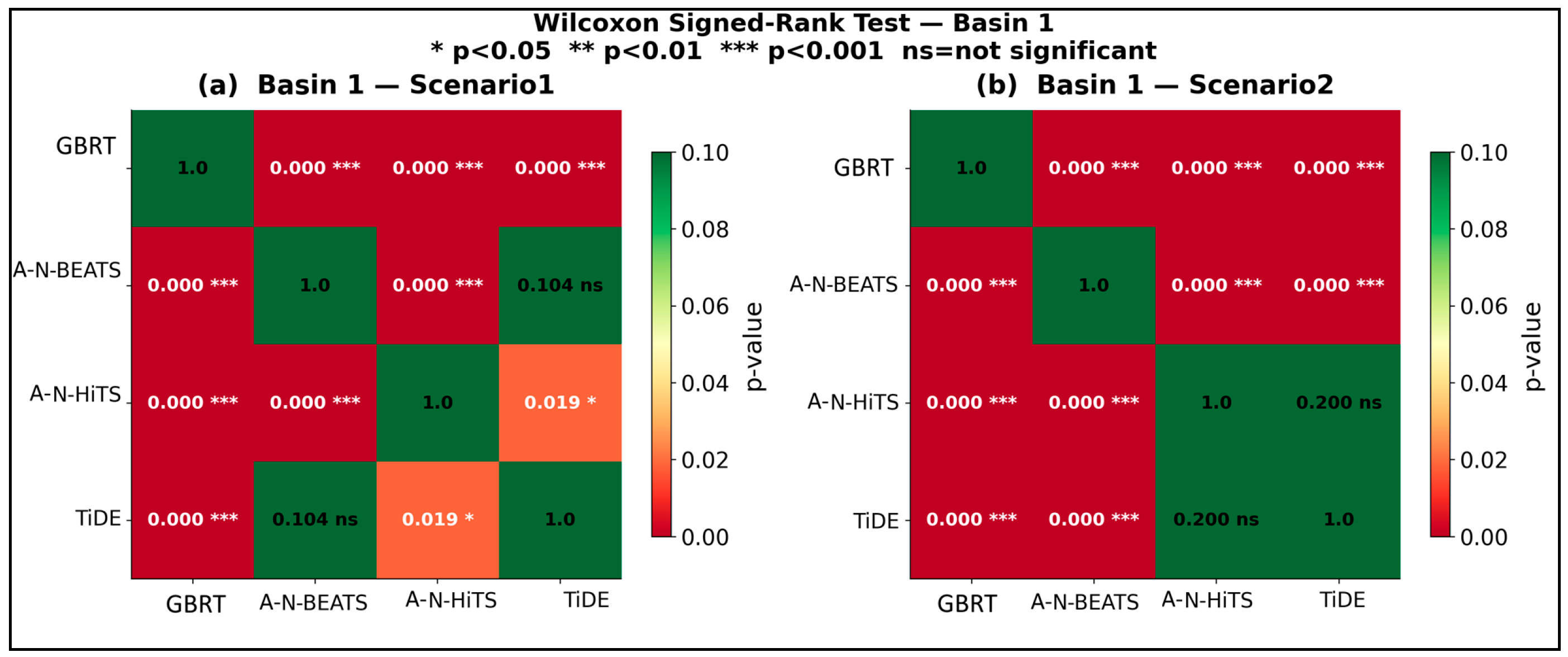
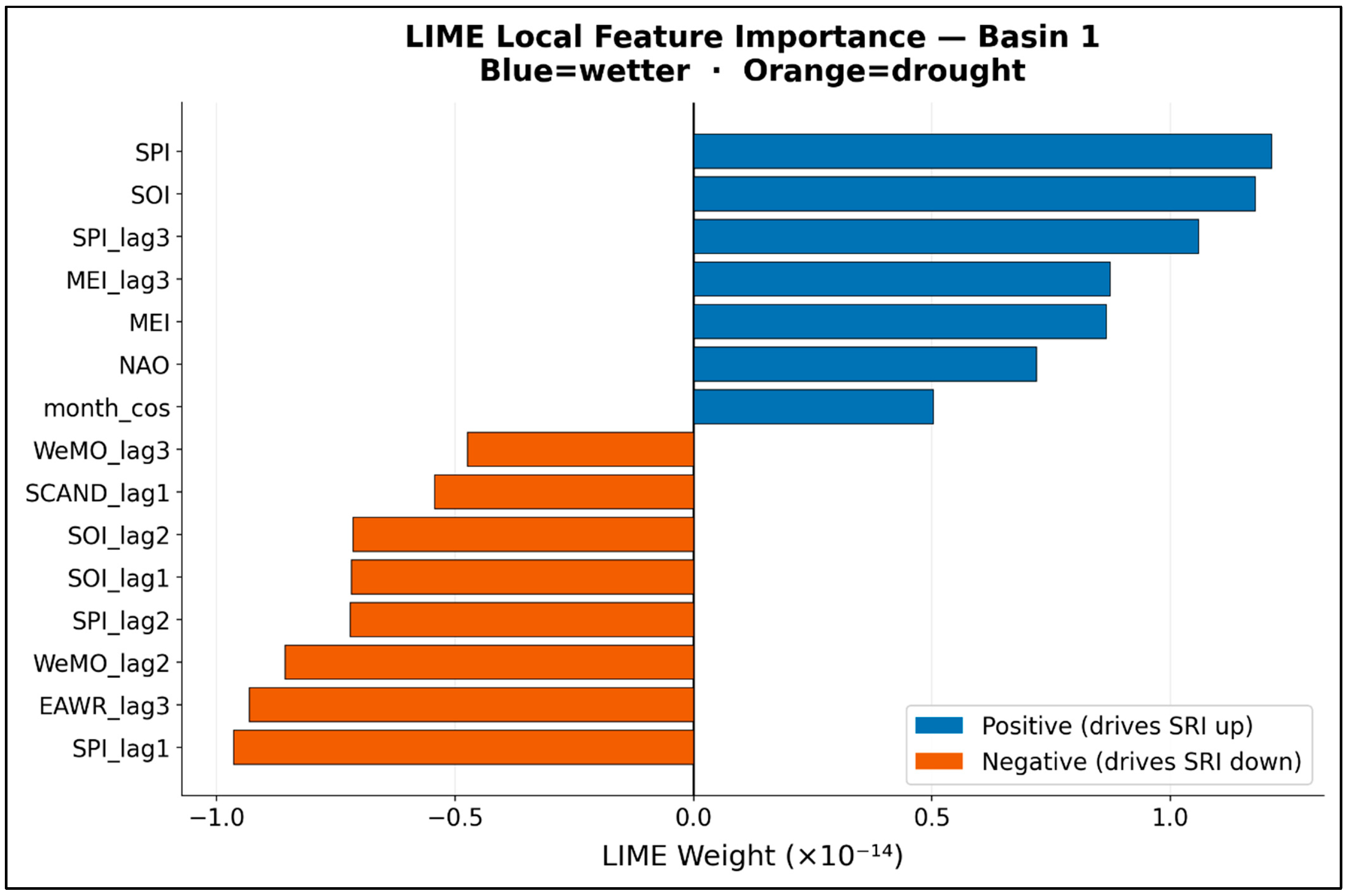
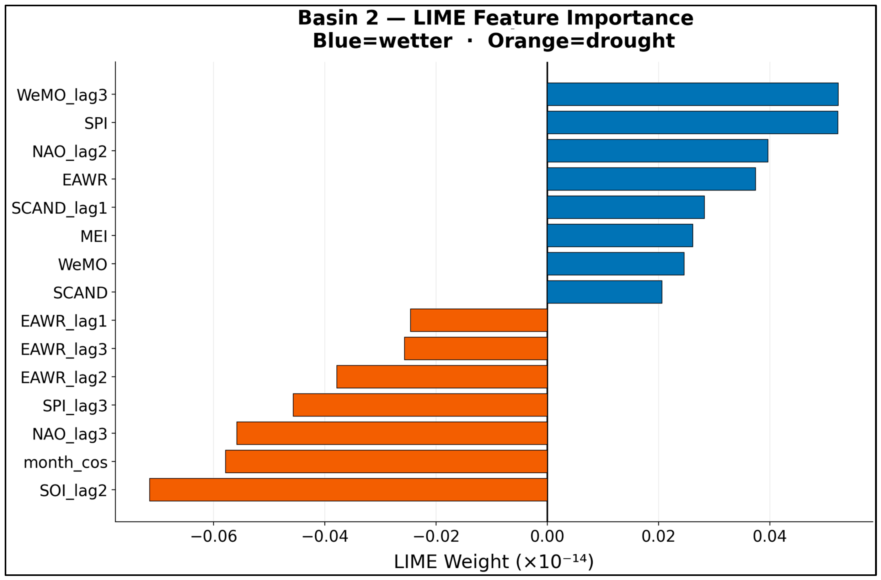
Figure 11, Figure 12, Figure 13 and Figure 14 suggest that while model performances are often statistically distinguishable, some models (particularly A-N-HiTS and TiDE) show comparable behavior under certain scenarios. The LIME analysis indicates that both current and lagged hydro-climatic variables contribute to predictions, with differences in feature importance patterns between basins.

The statistical tests generally support the performance-based ranking, particularly the stronger performance of GBRT in terms of RMSE, MAE, NSE, and KGE. Nevertheless, the interpretation of model differences is based primarily on the consistency of the evaluation metrics across basins and scenarios rather than on raw p-values alone. Cases with marginal p-values, such as TiDE versus A-N-HiTS in some scenarios, are therefore discussed as indicative rather than conclusive.

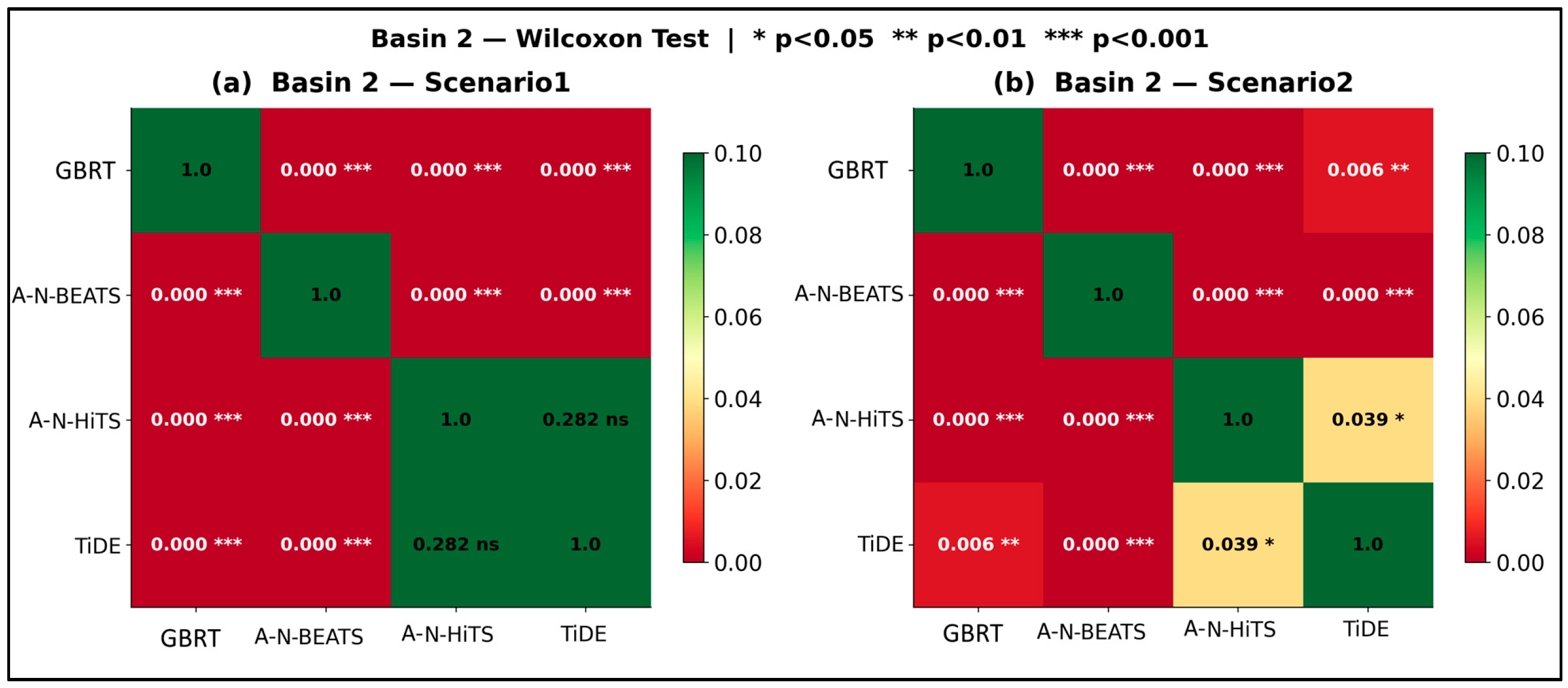
A similar pattern is observed. GBRT again shows statistically significant differences compared to other models in most cases (Figure 12). A-N-HiTS and TiDE appear statistically similar in Scenario 1 (p = 0.282), while in Scenario 2 the difference between them becomes marginally significant (p = 0.039). Additionally, GBRT and TIDE show a small but statistically significant difference in Scenario 2 (p = 0.006), which may suggest some convergence in performance compared to Basin 1. Given the high VIF values of some retained lagged SRI variables in Basin 2, the LIME-based local attributions should be interpreted primarily at the feature-group level rather than as isolated per-variable effects. Therefore, the relative contributions of correlated predictors such as SPI, SPI_lag1, and SPI_lag3 are discussed with caution.

Hyperparameter tuning was performed using a compact grid-search strategy on the validation subset in

Table 9. Optimal hyperparameters selected using the external chronological validation subset. For GBRT, the candidate configuration was selected according to external validation RMSE, while scikit-learn’s internal early-stopping mechanism used only a 10% subset of the training block. For the neural models, early stopping was based on the external validation loss.

Basin	Scenario	Model	Optimal Hyperparameters
Basin 1	Scenario 1	GBRT	n_estimators = 80; learning_rate = 0.05; max_depth = 4; subsample = 0.8
	Scenario 1	A-N-BEATS	hidden = 64; lr = 0.01; epochs = 150; patience = 20; dropout = 0.05; batch = 32
	Scenario 1	A-N-HiTS	hidden = 64; lr = 0.01; epochs = 150; patience = 20; dropout = 0.05; batch = 32
	Scenario 1	TiDE	hidden = 64; lr = 0.01; epochs = 150; patience = 20; dropout = 0.05; batch = 32
	Scenario 2	GBRT	n_estimators = 80; learning_rate = 0.05; max_depth = 4; subsample = 0.8
	Scenario 2	A-N-BEATS	hidden = 64; lr = 0.01; epochs = 150; patience = 20; dropout = 0.05; batch = 32
	Scenario 2	A-N-HiTS	hidden = 64; lr = 0.01; epochs = 150; patience = 20; dropout = 0.05; batch = 32
	Scenario 2	TiDE	hidden = 64; lr = 0.01; epochs = 150; patience = 20; dropout = 0.05; batch = 32
Basin 2	Scenario 1	GBRT	n_estimators = 80; learning_rate = 0.05; max_depth = 4; subsample = 0.8
	Scenario 1	A-N-BEATS	hidden = 64; lr = 0.01; epochs = 150; patience = 20; dropout = 0.05; batch = 32
	Scenario 1	A-N-HiTS	hidden = 64; lr = 0.01; epochs = 150; patience = 20; dropout = 0.05; batch = 32
	Scenario 1	TiDE	hidden = 64; lr = 0.01; epochs = 150; patience = 20; dropout = 0.05; batch = 32
	Scenario 2	GBRT	n_estimators = 80; learning_rate = 0.05; max_depth = 4; subsample = 0.8
	Scenario 2	A-N-BEATS	hidden = 64; lr = 0.01; epochs = 150; patience = 20; dropout = 0.05; batch = 32
	Scenario 2	A-N-HiTS	hidden = 64; lr = 0.01; epochs = 150; patience = 20; dropout = 0.05; batch = 32
	Scenario 2	TiDE	hidden = 64; lr = 0.01; epochs = 150; patience = 20; dropout = 0.05; batch = 32

. The search was intentionally kept small because the available monthly hydrological dataset was limited, and overly broad tuning could increase the risk of overfitting. For GBRT, two parameter combinations were evaluated: (i) n_estimators = 80, learning_rate = 0.05, max_depth = 4, and subsample = 0.8; and (ii) n_estimators = 100, learning_rate = 0.03, max_depth = 5, and subsample = 0.9. For the neural models, two configurations were tested: (i) hidden = 64, learning rate = 0.01, epochs = 150, patience = 20, dropout = 0.05, and batch size = 32; and (ii) hidden = 64, learning rate = 0.005, epochs = 150, patience = 20, dropout = 0.10, and batch size = 32.

The optimal configuration was selected according to the lowest validation RMSE. Early stopping was applied to the neural models by monitoring validation loss, with training stopped when no improvement was observed for 20 consecutive epochs. The maximum number of epochs was set to 150. For GBRT, the scikit-learn GradientBoostingRegressor internal early-stopping mechanism was used with n_iter_no_change = 15 and validation_fraction = 0.1. This internal validation subset was drawn only from the chronological training block and did not include observations from the external validation or test partitions. The external chronological validation set was used only to select the best GBRT candidate configuration based on validation RMSE. In contrast, early stopping for the neural models was performed directly by monitoring the external chronological validation loss. Therefore, the stopping mechanisms were model-specific, but the held-out test set remained completely unused during training, early stopping, and hyperparameter selection. Neural network weights were initialized using seed-controlled He-type random initialization. Therefore, the repeated appearance of identical optimal hyperparameters across basins and scenarios reflects the outcome of the validation-based selection process within a compact search space, rather than the use of arbitrarily fixed parameters.

The LIME-based local surrogate outputs were re-examined because the resulting feature weights were extremely small, approximately on the order of 10⁻¹⁴. At this numerical scale, the apparent ordering of predictors should not be interpreted as a robust local sensitivity ranking. Therefore, the LIME results were not used to draw strong conclusions about the dominance of individual predictors. Instead, Figure 13 and Figure 14 are interpreted only as diagnostic local surrogate outputs with limited explanatory value.

Consequently, the interpretation of model behaviour in this study relies primarily on the leakage-free performance evaluation, scenario comparison, and hydrologically meaningful metrics. The comparison between Scenario 1 and Scenario 2 remains useful for assessing the role of hydrological memory, whereas the LIME results are treated cautiously because the near-zero surrogate coefficients may reflect numerical instability or a degenerate local approximation.

Figure 11. Unadjusted Wilcoxon signed-rank test p-value heatmaps for exploratory pairwise comparisons of forecasting model errors in Basin 1 under Scenario 1 and Scenario 2. The p-values should be interpreted cautiously because monthly residuals may exhibit serial dependence.

Figure 11. Unadjusted Wilcoxon signed-rank test p-value heatmaps for exploratory pairwise comparisons of forecasting model errors in Basin 1 under Scenario 1 and Scenario 2. The p-values should be interpreted cautiously because monthly residuals may exhibit serial dependence.

Figure 12. Unadjusted Wilcoxon signed-rank test p-value heatmaps for exploratory pairwise comparisons of forecasting model errors in Basin 2 under Scenario 1 and Scenario 2. These heatmaps are used as supplementary diagnostics rather than definitive evidence of model superiority.

Figure 12. Unadjusted Wilcoxon signed-rank test p-value heatmaps for exploratory pairwise comparisons of forecasting model errors in Basin 2 under Scenario 1 and Scenario 2. These heatmaps are used as supplementary diagnostics rather than definitive evidence of model superiority.

Figure 13. LIME-based local surrogate output for Basin 1. Positive values indicate local contributions toward higher predicted SRI, whereas negative values indicate local contributions toward lower predicted SRI. Because the LIME weights are extremely small, approximately on the order of 10⁻¹⁴, the apparent feature ordering should be interpreted cautiously and should not be considered a robust predictor-importance ranking.

Figure 13. LIME-based local surrogate output for Basin 1. Positive values indicate local contributions toward higher predicted SRI, whereas negative values indicate local contributions toward lower predicted SRI. Because the LIME weights are extremely small, approximately on the order of 10⁻¹⁴, the apparent feature ordering should be interpreted cautiously and should not be considered a robust predictor-importance ranking.

Figure 14. LIME-based local surrogate output for Basin 2. Blue bars indicate positive local contributions associated with higher predicted SRI, whereas orange bars indicate negative local contributions associated with lower predicted SRI. Because the LIME coefficients are close to numerical zero, the plot is retained only as a diagnostic local explanation and is not used to infer dominant predictor effects.

Figure 14. LIME-based local surrogate output for Basin 2. Blue bars indicate positive local contributions associated with higher predicted SRI, whereas orange bars indicate negative local contributions associated with lower predicted SRI. Because the LIME coefficients are close to numerical zero, the plot is retained only as a diagnostic local explanation and is not used to infer dominant predictor effects.

4. Discussion

This study addresses a critical gap in hydrological drought forecasting by systematically evaluating both ensemble and deep learning approaches within a lagged multivariate supervised learning framework for one-month-ahead prediction of the SRI in two sub-basins of the Wadi Sahaouat Basin, Algeria. Four architecturally distinct models namely GBRT, A-N-BEATS, A-N-HiTS, and TiDE were compared to capture diverse learning paradigms. The predictor framework integrates both local and large-scale climatic drivers, including the SPI and key teleconnection indices such as the North Atlantic Oscillation, Arctic Oscillation, and El Niño–Southern Oscillation, along with their lagged effects. To explicitly assess hydrological memory, two scenarios were designed, with Scenario 2 incorporating lagged SRI, enabling a deeper understanding of antecedent basin conditions.

The dominance of GBRT in Basin 1 is strongly supported by existing literature emphasizing the robustness of ensemble tree-based methods under nonlinear and multicollinear conditions. For instance, Chen and Guestrin (2016) demonstrated the effectiveness of boosting algorithms in handling feature redundancy, while Mosavi et al. (2018) highlighted their superior performance in hydrological applications [44,45]. These findings are further reinforced by regional case studies: Achite et al. (2022) reported that ANN, SVM, and RF achieved high predictive accuracy (NSE up to 0.96), with hybrid ELM models further improving performance (NSE up to 0.98 and error reductions of 15–25%) in Algerian basins, demonstrating the effectiveness of ML approaches under semi-arid conditions [21]. Similarly, Pande et al. (2025) showed that models such as MLP and RF achieved NSE up to 0.96 and NSE > 0.90 with improved lead times, while Basak et al. (2022) highlighted the suitability of data-driven models like Prophet (NSE up to 0.92) in data-scarce regions [23,46]. Furthermore, Li et al. (2023) demonstrated that hybrid approaches (e.g., VMD-MLP, EEMD-RF) significantly enhance drought prediction accuracy (NSE up to 0.97), reinforcing the reliability of advanced ML frameworks across diverse climatic settings [47].

In contrast, the improved performance of deep learning models in Basin 2 under Scenario 2 highlights the critical role of hydrological memory. The exceptional performance of TiDE (KGE = 0.9878) is consistent with findings from Lim and Zohren (2021), who showed that encoder–decoder architectures excel when combining exogenous and autoregressive inputs [48]. This is further supported by the classical work of Hundecha and Bárdossy (2004), which established that hydrological systems exhibit strong temporal persistence [49]. Together with recent hybrid and deep learning studies, these results confirm that while ensemble models provide stable baseline performance, deep learning architectures can outperform them when basin memory is explicitly incorporated.

Despite its robust findings, this study has some limitations. The relatively short temporal dataset may not fully capture long-term variability associated with large-scale climate drivers such as the El Niño–Southern Oscillation and North Atlantic Oscillation. Additionally, the analysis is limited to two semi-arid basins, which may restrict broader applicability. Model performance also depends on feature selection and data quality, and the study does not fully explore global interpretability or causal mechanisms, suggesting avenues for future research.

The very high GBRT NSE values indicate that the monthly SRI series contains a strong predictable component under the selected feature design. However, this should not be interpreted as evidence that hydrological drought in a flashy semi-arid basin is nearly deterministic. Instead, the result likely reflects the combined effects of monthly aggregation, strong SPI–SRI coupling, short-term hydrological memory, and the capacity of GBRT to approximate nonlinear relationships among lagged hydroclimatic predictors. GBRT was included as a strong tree-based machine-learning benchmark against the adapted neural architectures, not as a naive hydrological baseline. Because persistence, climatology, AR(1), and ARIMA-type references were not included in the present experimental design, the absolute NSE values should be interpreted as model-set-specific performance rather than as a complete measure of practical forecasting improvement. Future studies should explicitly quantify the incremental value of the proposed framework relative to persistence and autoregressive baselines using rolling-origin validation and skill scores relative to persistence.

The paired t-test and Wilcoxon signed-rank test results were retained as exploratory diagnostics for pairwise model comparison. However, because the test period consists of monthly SRI forecasts, residuals and loss differences may exhibit serial dependence. Therefore, the raw p-values should not be interpreted as definitive evidence of model superiority.

The present modelling design should be interpreted as a targeted hydrological-memory experiment rather than as an exhaustive algorithmic benchmark. GBRT was included as the main strong tree-based benchmark against the adapted neural architectures. Scenario 2 intentionally incorporated SRI_lag1–3 to test whether antecedent hydrological conditions provide additional information beyond SPI, teleconnection indices, and seasonality. Because monthly SRI contains inherent temporal persistence, the high performance obtained in Scenario 2 should be interpreted with caution: it may partly reflect the exploitation of hydrological autocorrelation rather than a purely independent gain from exogenous predictors. Future work should extend this framework by including persistence, climatology, linear regression, AR/ARIMAX, random forest, XGBoost, and LightGBM under rolling-origin validation to quantify the incremental value of complex models over simple but strong reference forecasts.

A more rigorous time-series-aware significance assessment would require explicit reporting of loss-difference autocorrelation, effective sample size, moving-block bootstrap confidence intervals, and multiple-comparison-adjusted p-values. Since these adjusted quantities are not reported in the present version, they are discussed as a recommended extension rather than as evidence supporting the current conclusions.

The neural forecasting models evaluated in this study were adapted implementations inspired by the original N-BEATS, N-HiTS, and TiDE architectures. Therefore, the reported results should be interpreted as comparisons among the implemented model variants under a common experimental framework rather than definitive assessments of the original architectures. Consequently, conclusions regarding the relative performance of neural and boosting-based approaches are limited to the specific implementations, dataset, and experimental settings considered in this study. Although pairwise statistical tests were used to compare model performance, the results should be interpreted in conjunction with the magnitude of performance differences and their practical relevance. Statistical significance does not necessarily imply hydrologically meaningful improvements, particularly when multiple comparisons are performed and model performance metrics are already near their optimal values. Model evaluation was based on a chronological train–test split designed to preserve temporal consistency and avoid information leakage. While this approach reflects a realistic forecasting framework, additional validation strategies may provide further insight into model robustness. Therefore, the reported findings should be interpreted within the scope of the adopted validation design.

5. Conclusions

This study establishes an operationally relevant framework for monthly hydrological drought forecasting by integrating meteorological drought indicators (SPI), atmospheric teleconnection indices, and lagged SRI variables within a unified, leakage-free modelling pipeline. The results consistently show that gradient-boosted regression trees (GBRT) deliver the highest predictive accuracy across both basins and scenarios (mean RMSE = 0.0682; NSE = 0.9907), confirming their robustness for small-sample hydroclimatic applications with limited monthly observations.

A key finding is that the contribution of hydrological memory is strongly basin-dependent. In Basin 1, SRI lag variables were effectively redundant due to near-perfect collinearity with SPI (r = 0.984), indicating that meteorological forcing alone adequately captures hydrological drought dynamics. In contrast, in Basin 2, the inclusion of SRI lags led to clear performance improvements, most notably for the TiDE-inspired model, where KGE increased from 0.9372 to 0.9878. This result demonstrates that autoregressive runoff information can provide additional predictive value when it is not fully explained by precipitation-driven processes.

From a methodological perspective, the study further demonstrates that neural architectures adapted to lagged multivariate inputs can achieve competitive performance, although their advantages remain constrained under limited data availability and short memory structures. Overall, the findings underscore that effective model selection in hydrological drought forecasting depends not only on model complexity but also on data scale, basin-specific characteristics, and the degree to which hydrological memory contains independent information beyond meteorological forcing.

Although GBRT achieved the highest absolute accuracy among the tested models, its performance should be interpreted within the limits of the selected experimental design. The results suggest that gradient-boosted trees are effective in exploiting the short-term memory and SPI–SRI coupling present in monthly hydrological drought series. However, because persistence, climatology, AR(1), and ARIMA-type baselines were not included, the high NSE values should not be interpreted as standalone evidence of near-deterministic one-month-ahead drought predictability. The practical improvement over simple memory-based forecasts remains an important issue for future work.