1. Introduction
Statistical methods are essential tools for climate prediction, especially for longer lead times [
1,
2,
3]. Compared to traditional linear statistical methods such as multivariate linear regression, machine learning approaches are increasingly employed in climate prediction research due to their ability to capture complex nonlinear relationships [
4,
5,
6,
7]. Moreover, ongoing advancements in prediction systems that employ machine learning methods are consistently pushing the predictive skill ceiling upward [
8,
9,
10].
Unlike many other machine learning domains where model training benefits from abundant data, climate prediction is challenged by the scarcity of observed event samples, owing to the limited availability of reliable observations. For most climate events, the observation period is typically too short (less than 100 years) to yield an adequate quantity of samples used for model training. Addressing the challenge of a limited number of climate event samples, two main approaches are generally adopted. The first approach relies on numerical climate models: if these models can provide simulations that generally match observations, simulated data can be used to expand the training set, making it feasible to employ relatively complex machine learning models [
11,
12,
13,
14]. The other approach uses only observational samples; in this case, simpler machine learning models, typically containing only a few dozen parameters, are preferred, such as the widely applied artificial neural networks (NN) [
15,
16,
17]. This study focuses exclusively on the latter approach. This is primarily because, at the initial stage of investigating specific issues such as model stability, the use of simple models and small datasets minimizes computational costs, which, in turn, facilitates extensive testing and in-depth analysis.
For machine learning models, due to the use of random numbers (i.e., randomness) during the construction process, the final trained model obtained from each run varies (i.e., irreproducibility), resulting in differing model performance, and such instability becomes more pronounced in scenarios with a small sample size [
18,
19,
20]. In recent years, a few studies have highlighted the non-negligible impact of randomness on model performance in such contexts [
21,
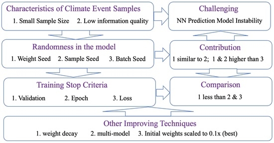
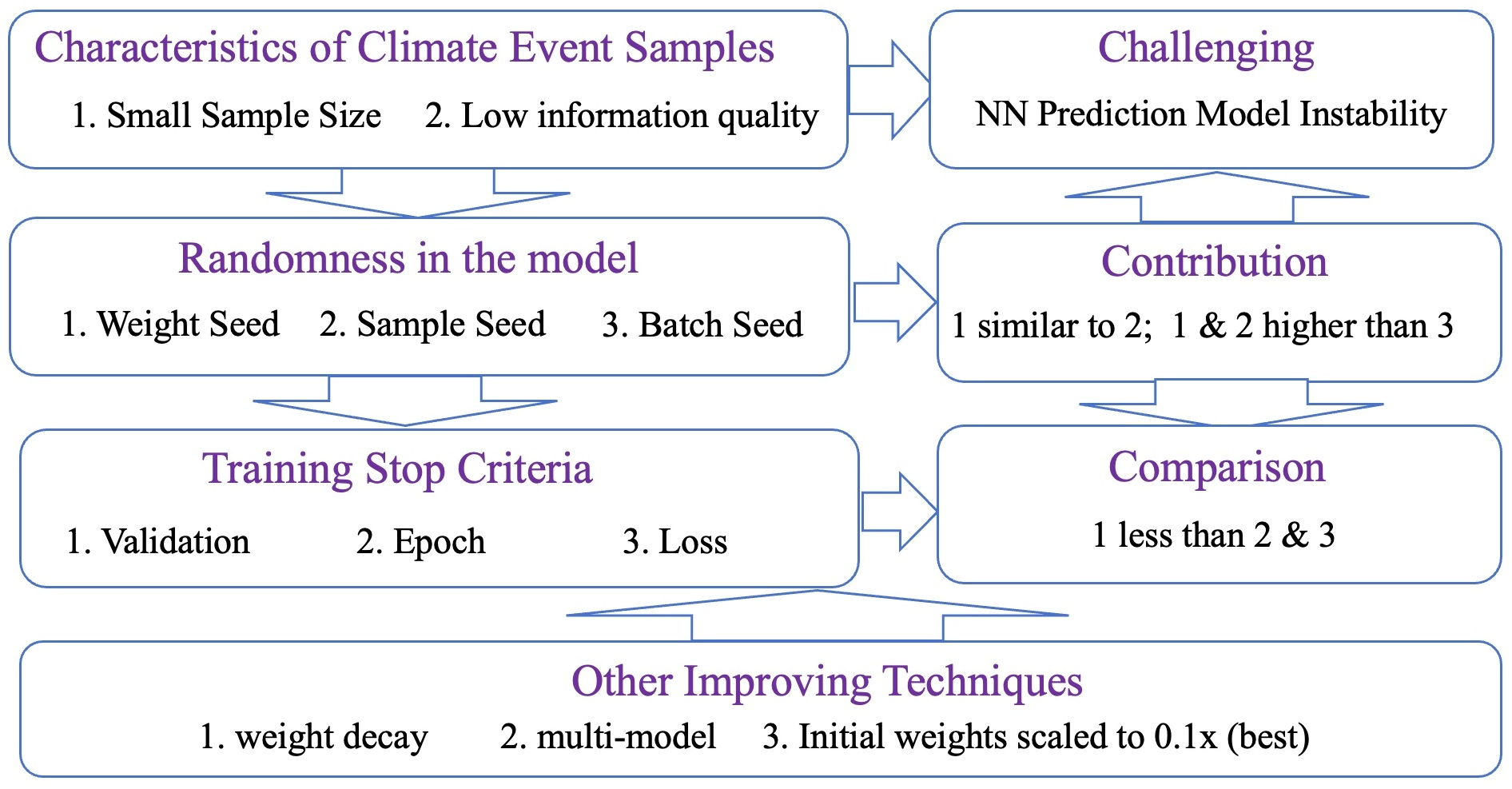
22]. Beyond the challenge of limited sample size, climate event data are also characterized by low information quality. Specifically, the predictors used as model inputs influence the target variables (i.e., predictions) only to a limited extent, implying a weak statistical relationship between them. As an example, consider the prediction of July precipitation over the middle and lower reaches of the Yangtze River (MLYR) using early winter sea surface temperature (SST) anomalies as predictors. Although El Niño-like SST anomalies in the preceding winter increase the likelihood of above-normal July precipitation, there are also years in which precipitation is below normal (e.g., 1966 and 2019). This behavior differs from that observed in many other machine learning applications. In handwritten digit recognition, for instance, images of the digit “1” are consistently associated with the target label “1”. Climate event prediction, by contrast, is intrinsically probabilistic; consequently, insights drawn from other domains may not be applicable here. Motivated by the combined challenges of small sample sizes and low information quality, this study systematically investigates the sources of instability in NN models, quantifies their relative contributions, and proposes targeted mitigation methods, thereby supporting the construction of more robust NN-based climate prediction models.
To facilitate experimental analysis at the preliminary research stage, this study employs a typical climate prediction task by using the prediction of July precipitation in the MLYR based on early winter SST as a case study. This paper is structured as follows.
Section 2 introduces the NN model and experimental setup. Results and analysis are presented in
Section 3.
Section 4 discusses how the findings introduced here can be applied, while
Section 5 concludes the paper.
2. Data and Methods
2.1. Samples for the NN Model
The original station-observed monthly precipitation data from 1951 to 2021 are provided by the National Climate Center of the China Meteorological Administration. First, July precipitation values from all 15 stations in the MLYR region (28.50° N to 32.00° N, 106.48° E to 118.80° E) are averaged into a single value. Next, the decadal trend is removed, and precipitation anomaly percentages are calculated. Finally, these percentages are amplified for extreme events and normalized to the range of −1 to 1; details of this procedure and the underlying rationale are provided in Jiang and Shi (2023) [
23]. Hereafter, this indexed precipitation is denoted as Rain. The original monthly SST data are obtained from the IRI/LDEO Climate Data Library [
24]. Since the primary indicative winter SST signals originate from the Pacific and Indian Oceans [
25,
26], winter mean SST anomalies from the corresponding domain (40° S to 60° N, 30° E to 90° W) are used to extract predictor variables. Following previous studies [
15,
16,
23,
27], SST principal components (PCs) serve as potential predictors. From 1951 to 2021, there were a total of 71 climate events (one per year). Each event corresponds to one sample, consisting of one Rain value (i.e., one predictand) and 30 SST PCs (i.e., 30 potential predictors).
Appendix A provides more details of the sample data. Furthermore, the data values can be downloaded according to the Data Availability Statement.
2.2. The NN Prediction Model
Here, a two-layer NN with relatively few tunable parameters is chosen for the prediction model. The number of nodes in the input layer, first hidden layer, and second hidden layer are denoted as Nx, N1, and N2, respectively. The model outputs only one variable (i.e., the predicted Rain). The default model architecture is configured as Nx = 6, N1 = 8, N2 = 3. The number of predictors used in the NN model cannot exceed 30 (i.e., Nx ≤ 30). Under Nx < 30, the PCs are prioritized based on the absolute value of their linear correlation coefficient (Cor) with Rain, with those having higher correlations selected first.
The NN model employs the tanh activation function. At model initialization, all biases are initialized to zero. Weights are initialized with random values drawn from a normal distribution, with the standard deviation set to
(where n denotes the number of nodes in the layer), similar to the commonly used Xavier initialization [
28]. During model training, the gradient is computed using the backpropagation algorithm with a batch of randomly selected samples. The batch size is set to 10. The initial learning rate is set to 0.01, and it is adaptively adjusted throughout the training process based on gradient dynamics via the Adam optimizer [
29].
During model training, the model’s performance is quantified by a loss function, defined as the Root Mean Squared Error between model predictions and observations (referred to as Loss hereafter). Given the small sample size and the limited predictive power of winter SST for July Rain, excessive model training will inevitably result in overfitting. Considering this, three training stopping criteria are available: Validation, Epoch, and Loss. If the Validation criterion is chosen, the train-dev set (i.e., the raw training set, including validation samples) is first randomly split before model training: two-thirds for model training, and the remaining one-third as the validation set. Both the Epoch and Loss are commonly used early stopping criteria, which do not require the validation set [
30]. Model training is stopped when the preset threshold is reached. To better compare model performance among these three stopping criteria, the default Loss threshold is set to 0.4, and the default epoch number threshold is set to 10. When adjusting the NN architectures or applying stabilization techniques, the default epoch number threshold may need to be adjusted to ensure that the model performance under the three stopping criteria remains approximately comparable.
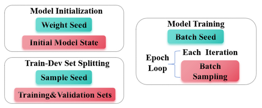
The construction process of the NN model can be divided into three independent procedures.
Figure 1 illustrates the randomness factors and corresponding random seeds in each procedure. Upon entering each procedure, the randomness factors can be controlled by setting a specific random seed. For instance, a given weight seed corresponds to one initial state of the model. The train-dev set splitting procedure is only applied when the Validation stopping criterion is used. During model training, each parameter update (i.e., each iteration) is based on a batch of randomly sampled samples. The batch seed, which is set before training begins, determines the batch sampling sequence for every iteration within each epoch. Overall, by setting these random seeds, the entire model construction process is reproducible.
Two simple techniques that enhance stability are introduced into the model: Weight Decay and Initialization0.1. When the Weight Decay technique is applied, all weights and biases are scaled by a decay factor of (1 − λ) at each iteration. The decay coefficient λ is set to 0.02. The method used here differs from the standard L2 regularization formulation prevalent today (which applies penalties via the loss gradient), representing a relatively older implementation. Unlike off-the-shelf tools, our custom-coded approach allows for more flexible handling of the processing details. If the norm of all model parameters falls below a very small threshold (0.1), the Weight Decay mechanism is disabled by setting λ to 0. Conversely, when the norm is large, λ is doubled to enhance its effect. The Initialization0.1 technique is straightforward: it simply scales all weights from the default initialization down to one-tenth (i.e., 0.1) of their original values. Beyond the value of 0.1, we tested a range of scaling coefficients (1 × 10
−6, 0.05, 0.1, 0.2, and 0.5). Given that performance plateaued below 0.1, we selected 0.1 for this study. In addition to the two techniques mentioned above, ensemble experiments are also employed to enhance the stability of the forecast results. This multi-model ensemble method will be introduced in
Section 2.3.
To facilitate memorization of the NN model’s configuration,
Table 1 lists all configuration options relevant to the subsequent experiments. If there are no specific instructions, the default settings are used. Moreover, the NN model and all its subroutines (e.g., the random number generator) are coded in Fortran by the authors. Technical details can be found in the source code, which is available for download according to the Data Availability Statement.
2.3. Experimental Settings and Evaluation Metrics
The options for the experimental setup are summarized in
Table 2. This study conducts two types of experiments: Single and Ensemble. In an Ensemble experimental run, the only difference between individual ensemble members is the random seeds used, which is consistent with the repeated runs in a Single experiment. In this study, each experiment (both Single and Ensemble) comprises 30 repeated runs. By default, the experiments reported are Single experiments. To demonstrate how different ensemble sizes affect model stability, the number of ensemble members is variable and specified for each corresponding experiment.
Given the differences in model’s performance between the training and testing sets, three experimental strategies have been designed: OnlyTrain, TrainTest, and LOO. In the OnlyTrain strategy, all samples are used to train the model when using the Epoch or Loss training stopping criteria. When the Validation training stopping criterion is adopted, a portion of the samples is reserved as a validation set. In experiments using this strategy, only the model’s performance on the train-dev (training) set is provided. Typically, greater attention is placed on the model’s performance on the test set, as it provides a more rigorous and generalizable assessment of the model’s predictive skill for unseen future events. In the TrainTest strategy, 45 out of the total 71 samples are used as the train-dev (training) set, and 26 as the test set. The results from experiments using this strategy allow for a comparison of the model’s performance between the train-dev (training) and test sets. The LOO strategy refers to the well-known Leave-One-Out cross-validation experiment. In each independent run, it selects one sample as the test set and uses the remaining samples as the train-dev (training) set, repeating this process until every sample has served as the test set once. Compared to the TrainTest experiment, whose results are subject to the influence of the specific train-dev/test set split, the LOO experiment provides a more robust evaluation of the model’s predictive skill.
In addition to the Loss, the model’s performance is also evaluated using the Cor, a metric commonly employed in climate prediction models. To analyze the model stability, each experiment (both Single and Ensemble types) is repeated 30 times, with the only variation being the random seeds used. Each experimental run produces one prediction model (which can be either a single model or an ensemble model), from which a pair of Loss and Cor scores is obtained. The reported Loss and Cor scores are the mean values across all 30 runs, accompanied by their corresponding standard deviations (presented as mean ± std.). Furthermore, an additional metric has been designed to quantify the stability (hereafter Sta). For each sample, a standard deviation value can be calculated based on the model-calculated Rain from these 30 runs. The “Sta” score is defined as the average of these standard deviation values across all samples in the dataset. It is evident that a higher Sta indicates poorer stability. It is worth noting that conducting 30 runs for the LOO experiment entails a significant number of model trainings (71 × 30 = 2130). Undoubtedly, the Sta score becomes more robust with an increasing number of repeated runs. Here, we set the number of runs to 30 to balance accuracy and computational cost. As demonstrated by five preliminary experimental groups, the Sta scores (0.136, 0.129, 0.128, 0.130, and 0.135) remained acceptably consistent. Finally, it is essential to point out that the model stability (instability) discussed in this study specifically refers to the model’s performance (i.e., model-calculated Rain) rather than the model’s parameters (i.e., weights and biases).
3. Results and Analysis
In this section, the impact of randomness factors (i.e., random seeds) on the model construction process is first tested. Next, the relative contribution of each randomness factor to the model instability is assessed. Subsequently, the potential factors influencing model stability are investigated. Finally, techniques for enhancing stability are evaluated.
3.1. Training Process Analysis
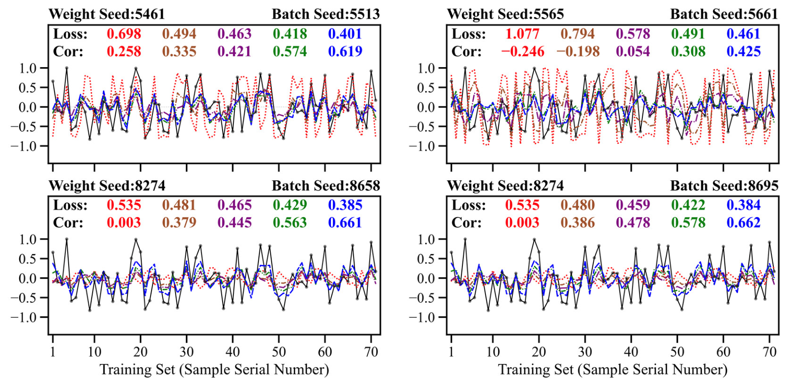
Here, the impact of different weights and batch seeds on the model training process (including both the initial and final states) is demonstrated through the OnlyTrain experiments with the Epoch stopping criterion (
Figure 2). During the first two epochs (brown and purple), the model shows significant improvements in the Loss and Cor scores, which is likely due to the learning rate of 0.01, which is not particularly small. From epochs 5 (green) to 10 (blue), the model-calculated Rain continues to show improvements in scores. However, a closer look at the Rain values (represented by the green and blue lines) reveals that the improvements are no longer pronounced, as the two lines overlap considerably. This suggests that the model performances do not improve in a relevant manner when the epoch number threshold (10) is approached. It is clear that the model’s initial state is entirely controlled by the weight seed. The initial scores (red color) are identical for a given weight seed (8274, the second row). Due to the randomness of the initial states, the Cor scores can be either positive or negative. The loss scores are generally not small (e.g., the first row), with the vast majority being above the standard deviation of the target variable Rain (0.509). Excluding the training process in the lower-right panel (since its Weight Seed is identical to the previous one), the final scores (blue color) of the three models differ markedly (Loss 0.401, 0.461, and 0.385; Cor 0.619, 0.426, and 0.661), likely due to notable differences in their initial states. It appears that a poor initial state likely leads to inferior performance even after 10 epochs of training. The second row shows the variation in the performances and scores for models trained using weight seed 8274 and two different batch seeds. Although the final (10th epoch) Loss and Cor scores vary among these two models (Loss 0.385 and 0.384; Cor 0.661 and 0.662), the differences are not pronounced. Generally speaking, the impact of batch seeds is much less pronounced than that of weight seeds.
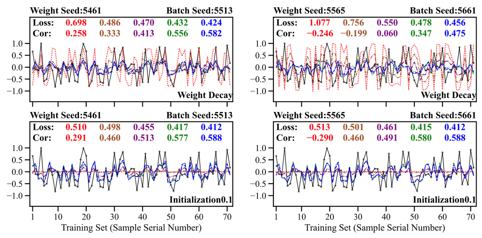
Figure 3 shows training processes with two stabilization techniques. The first row shows two model training processes with Weight Decay. Compared to the two NN models without Weight Decay (the first row of
Figure 2; final score Loss 0.401, Cor 0.619; Loss 0.461, Cor 0.426), the difference in final scores between the two sets of random seeds is reduced (Loss 0.424, Cor 0.582; Loss 0.456, Cor 0.475). With the Initialization0.1 (the second row), all initial weights are scaled by a factor of 0.1 with respect to their original values. As long as the activations remain within the non-saturated (i.e., approximately linear) regime of the tanh function, the signal amplitude is attenuated to roughly 1/1000 of its original scale after propagating through one input layer and two hidden layers. Therefore, with this technique, the initial model-calculated Rain is near zero. In such a scenario, the initial Loss is essentially the standard deviation of Rain (0.509). This is the reason why the obtained two initial Loss values (0.510 for seed 5461, 0.513 for seed 5565) align closely with each other. While the Initialization0.1 technique compresses the initial model-calculated Rain near zero, the Cor scores (0.291 for seed 5461 and −0.290 for seed 5565) do not change considerably compared to the models with the same seeds but without Initialization0.1 (the first row of
Figure 2; 0.258 for seed 5461 and −0.246 for seed 5565). This occurs because linear correlation focuses on the consistency of variation trends between the two sequences rather than their absolute values. Due to the Initialization0.1 technique compressing the initial model-calculated Rain near zero, which makes it nearly unaffected by the weight seed, the final scores from the two different sets of random seeds (Loss 0.412, Cor 0.588; Loss 0.412, Cor 0.588) become nearly identical (the bottom row). Overall, both the Weight Decay and Initialization0.1 techniques could improve the stability of the final trained models.
3.2. Contribution of Different Random Seeds to Model Instability
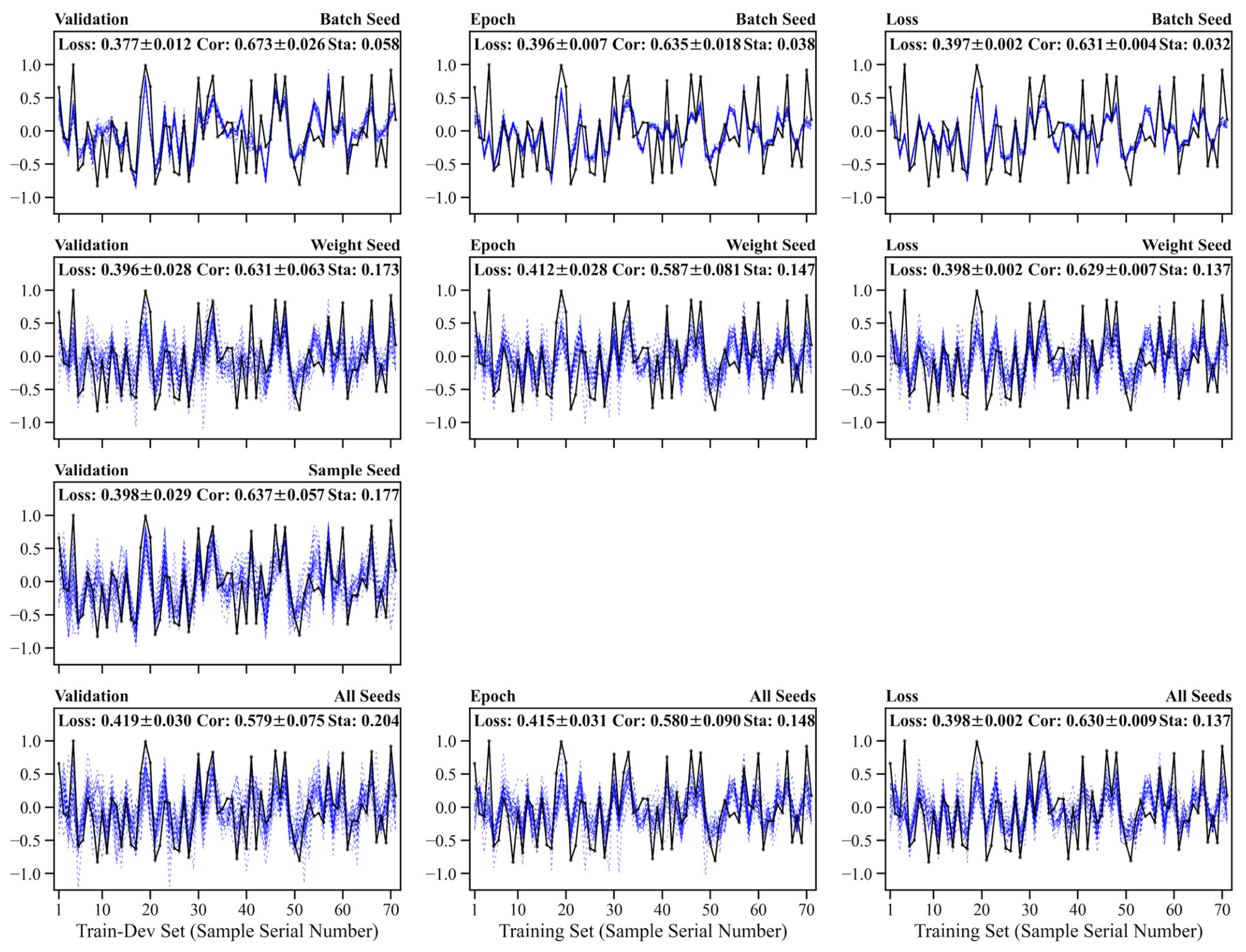
By controlling random seeds as fixed or variable, the impact of a specific random seed on the final trained model can be individually analyzed. Here, the experimental category still adopts OnlyTrain, but all three training stopping criteria are used (
Figure 4).
Regardless of the stopping criteria used, the instability induced by batch seeds (first row, Sta 0.058, 0.038, and 0.032) is considerably weaker than that induced by weight seeds (second row, Sta 0.173, 0.147, and 0.137). Among them, the models using the Validation stopping criterion exhibit stronger instability (Sta 0.058 and 0.173) than those employing either the Epoch (Sta 0.038 and 0.147) or Loss stopping criteria (Sta 0.032 and 0.137). One possible reason is that using the validation set to determine when to stop introduces additional complexity into the model training process, which, in turn, makes it more sensitive to random events. The third row demonstrates how model performance varies with different splits of the train-dev set into training and validation subsets (determined by the sample seed). The model instability induced by sample seeds is obvious, with a comparable magnitude (Sta 0.177) to that from weight seeds (Sta 0.173, second row). The bottom row illustrates the instability contributed by all random seeds. Experiments using both the Epoch and Loss stopping criteria are influenced only by weight seeds and batch seeds. The model instability resulting from these two seeds (Sta 0.148 and 0.137) is similar to that induced by the weight seeds alone (Sta 0.147 and 0.137). For the Validation stopping criterion, the model instability resulting from all random seeds (Sta 0.204) is markedly higher than that induced by any single seed type alone (Sta 0.058, 0.173, and 0.177). Overall, the instability induced by validation seeds or weight seeds is much stronger than that induced by batch seeds. Furthermore, the model demonstrates higher instability when employing the Validation stopping criterion compared to the Epoch or Loss criteria.
This paragraph analyzes the stability from the perspective of the std. values of Loss and Cor scores. Under the Validation and Epoch stopping criteria, the std. value generally tracks Sta, rising and falling with it. In other words, the instability of Loss and Cor scores generally covaries with that of the model-calculated Rain (i.e., Sta). However, this general expectation does not apply when using the Loss stopping criterion. The use of a Loss stopping criterion (threshold = 0.4) truncates the distribution of final Loss scores, artificially clustering them just below 0.4, which naturally results in a very stable Loss score. In the three experiments that used the Loss stopping criterion (first row, second row, and fourth row of the right column), the std. values of Loss scores are all 0.002, regardless of whether the model-calculated Rain exhibits significant instability. Since the Cor score is correlated with the Loss score, it remains relatively stable as well. Specifically, the std. values of the Cor scores are all below 0.009, which are much lower than those from the experiments using the Epoch stopping criterion. It is noteworthy that the Loss stopping criterion contributes to more stable scores on the training set rather than to more stable model performance (i.e., model-calculated Rain). This distinction highlights an important insight: stable loss scores do not necessarily imply stable model behavior.
3.3. Multi-Perspective Analysis of Model Performance
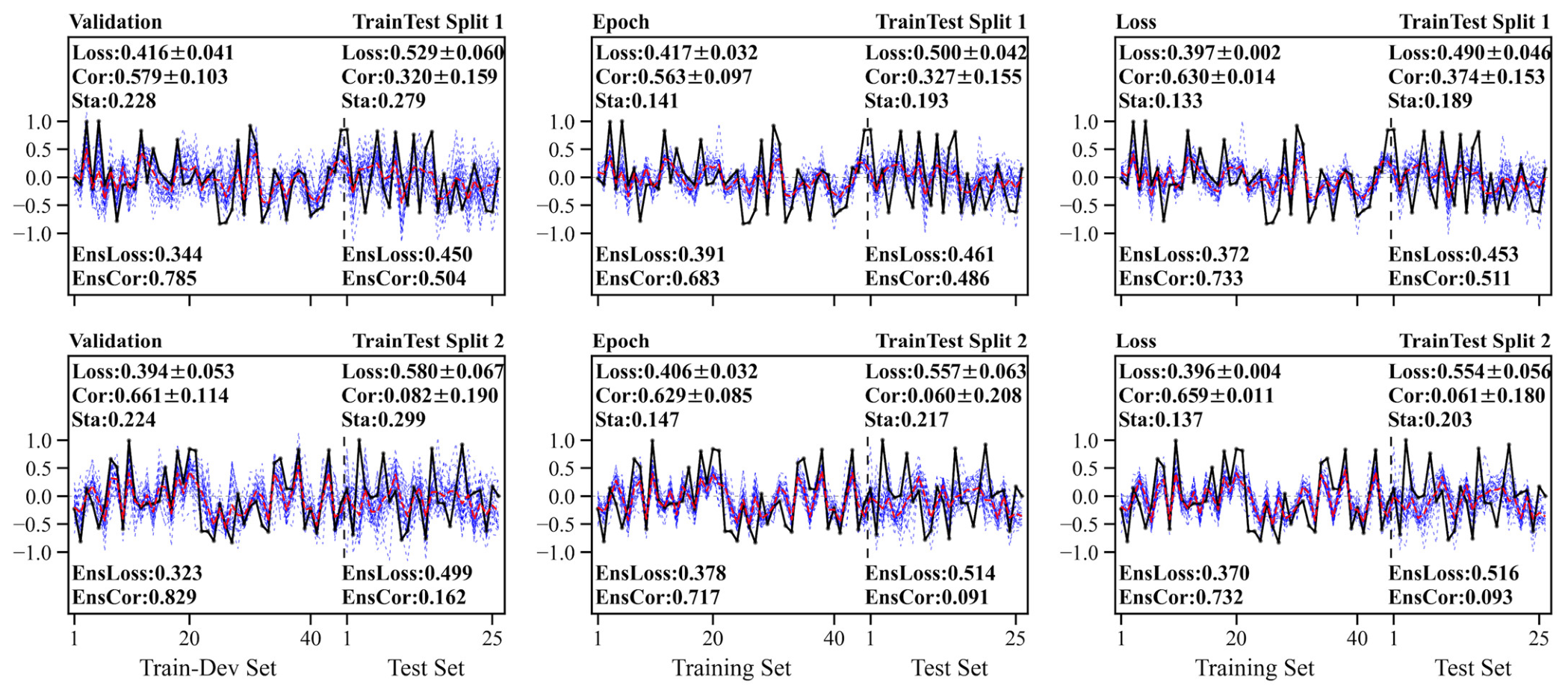
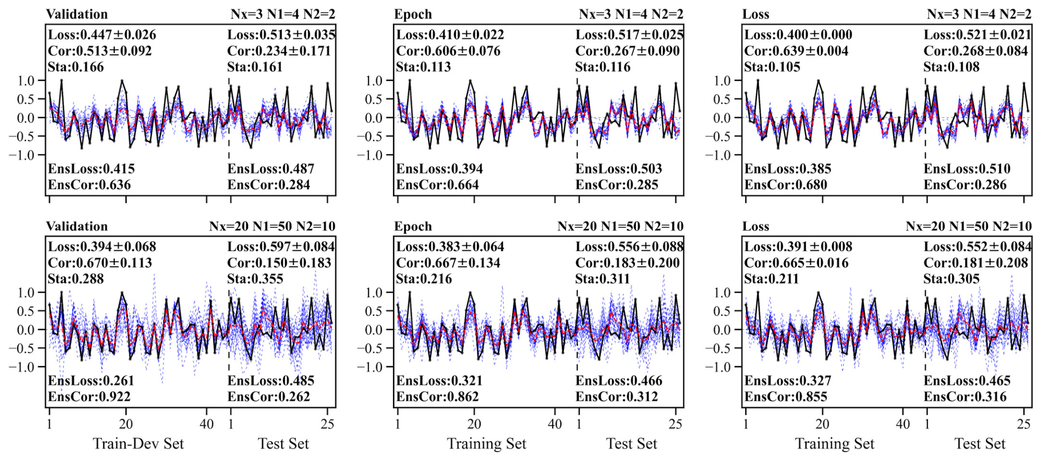
Here, the difference in model stability between the train-dev (training) and test sets is analyzed using the TrainTest category with all random seeds varied (
Figure 5). Considering the potential impact of different train-dev (training) and test set splits, two distinct dataset partitions are presented here. One partition represents a common or typical scenario (first row), while in the other, the model’s scores on the test set are very poor (second row). As expected, the model exhibits noticeably weaker stability (i.e., higher Sta value) on the test set than on the train-dev (training) set, regardless of the dataset partition or stopping criterion used. Moreover, when test set performance is particularly poor, as in the second partition, its stability is also substantially worse. Similar to the above analysis in
Section 3.2, the Validation experiments show worse stability than the Epoch and Loss experiments, on both the train-dev and the test sets.
This paragraph further analyzes the model’s performance from the perspective of the Loss and Cor scores. When the Loss stopping criterion is used, although the Loss and Cor scores are stable on the training set, the std. values on the test set increase markedly, approaching the results calculated from experiments using the Epoch stopping criterion. In the first row of
Figure 5, the model’s scores on the train-dev set from the Validation experiment (Loss 0.416 ± 0.041; Cor 0.579 ± 0.103) are worse than those from the Loss experiment (Loss 0.397 ± 0.002; Cor 0.630 ± 0.014). However, when analyzed based on the average of the model-calculated Rain from these 30 repeated runs (i.e., as one ensemble experiment), the ensemble model scores of the Validation experiment (Loss 0.344; Cor 0.785) are better than those of the Loss experiment (Loss 0.372; Cor 0.733). This suggests that the worst stability of the single model (Validation experiments) might be beneficial for achieving better ensemble model scores. Similarly, although the individual model scores on the test set from the Validation experiment (Loss 0.529 ± 0.060; Cor 0.320 ± 0.159) are worse than those from the Epoch experiment (Loss 0.500 ± 0.042; Cor 0.327 ± 0.155), the ensemble model scores from the Validation experiment (Loss 0.450; Cor 0.504) are better than the Epoch experiment (Loss 0.461; Cor 0.486). At last, it is noteworthy that ensemble averaging can substantially improve the model’s scores, which is consistent with ensemble diversity theory (e.g., Hansen and Salamon 1990; Krogh and Vedelsby 1995) [
31,
32].
The influence of model capacity is illustrated using the experimental results from two distinct NN architectures (
Figure 6): a simple architecture (
Nx = 3,
N1 = 4,
N2 = 2) and a complex architecture (
Nx = 20,
N1 = 50,
N2 = 10). As expected, compared to low-capacity models, high-capacity models exhibit stronger fitting capabilities on the train-dev (training) set but suffer from more severe overfitting issues. In terms of stability (i.e., Sta score), high-capacity models perform markedly worse (higher Sta values) than their low-capacity counterparts, especially on the test set. Low-capacity models maintain similar stability levels on the test and train-dev sets, whereas high-capacity models show a substantial drop in stability on the test set relative to the train-dev set. On the test set, the scores (Loss and Cor) of high-capacity models are markedly worse than those of low-capacity models. However, this conclusion may not hold when evaluated based on ensemble model scores. Taking the Epoch experiments as an example, the ensemble model score with the complex architecture (Loss 0.466; Cor 0.312) is better than that with the simple architecture (Loss 0.503; Cor 0.285). This again indicates that weaker stability may be beneficial for improving scores via ensemble experiments.
3.4. Different Techniques for Enhancing Model Stability
Model ensemble is a commonly used technique to enhance predictive reliability as well as mitigate the instability caused by randomness [
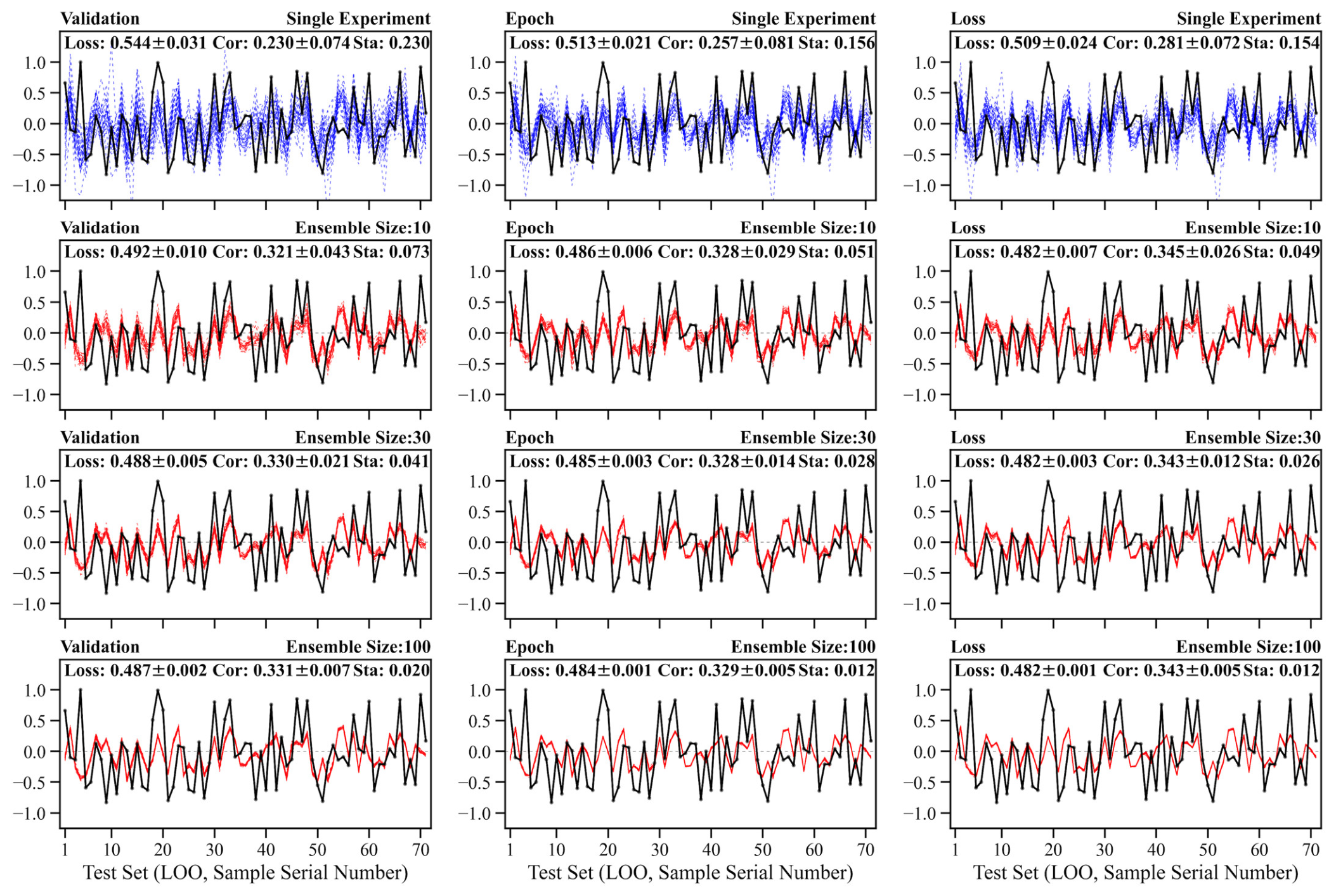
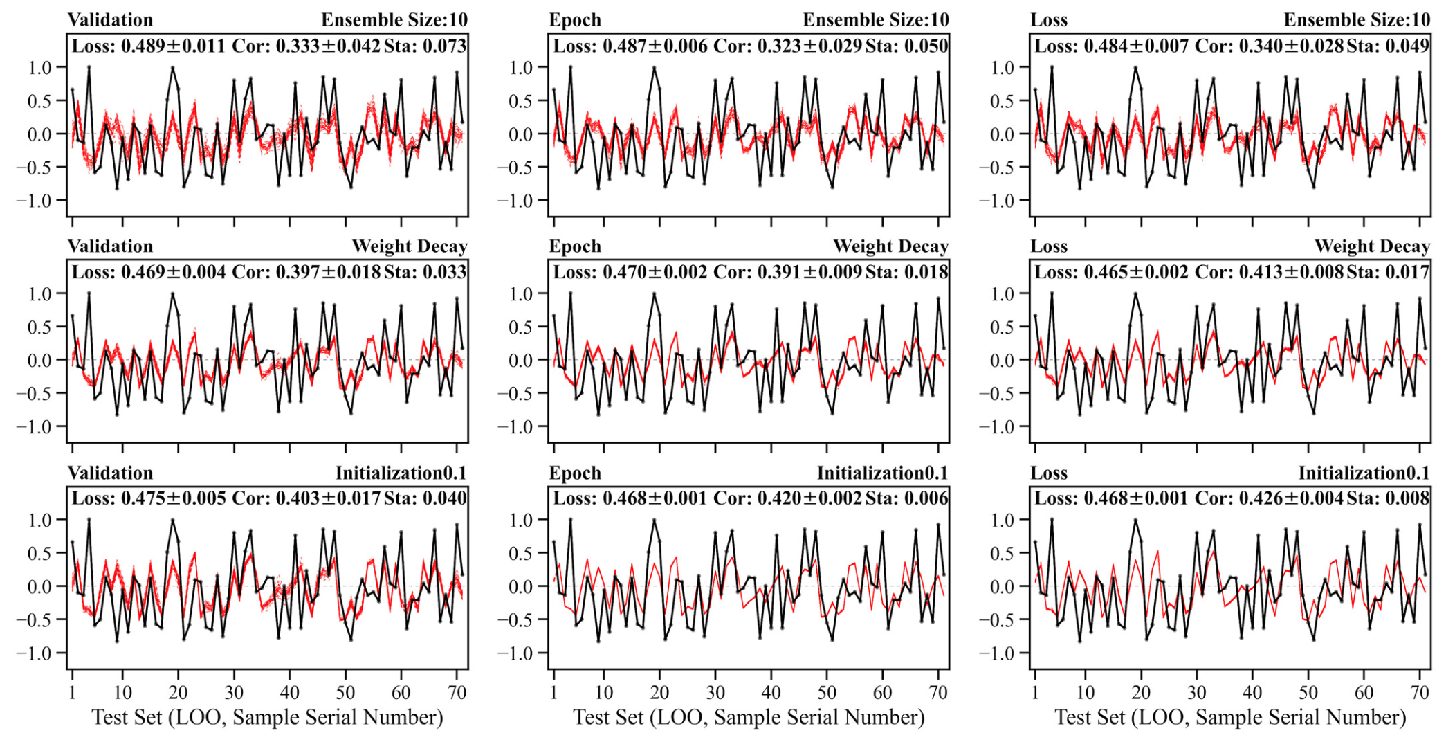
33]. Since practical applications demand stable performance on future (i.e., test set), we adopt the LOO experimental category for a more rigorous evaluation.
Figure 7 demonstrates how different ensemble sizes influence model stability. The Loss and Cor corresponding to the three stopping criteria are close to each other. However, the Sta for the Validation stopping criteria is substantially higher than that for the other two stopping criteria (Epoch and Loss). This once again confirms the conclusion drawn from the previous analysis. In the figure, single experiments can be viewed as ensemble experiments with an ensemble size of 1. According to probability theory, if the data follow a normal distribution, then after ensemble averaging, the standard deviation becomes 1/
times the original standard deviation, where n is the ensemble size [
34]. For the validation experiments, the Sta values are 0.230, 0.073, 0.041, and 0.020 for ensemble sizes of 1, 10, 30, and 100, respectively. These results are generally consistent with the probability theory introduced above. Note that, from ensemble size = 1 to ensemble size = 100, the Sta value dropped by more than 10 times, i.e., from 0.230 down to 0.020. For both the Epoch and Loss experiments, the Sta values are also dropped by more than 10 times. One possible reason is that the Sta value here is not the standard deviation on a single sample, but rather the average of standard deviations across all samples. In summary, based on the probability theory introduced above, we can roughly estimate the improvement in stability achieved by increasing ensemble sizes. The actual improvement may exceed this rough estimate.
Figure 8 illustrates the effects of the two techniques: Weight Decay (second row) and Initialization0.1 (third row). To facilitate comparative analysis, the first row shows the reference experiment. It is clear that both the Weight Decay and Initialization0.1 techniques markedly enhance model stability. For experiments using the Epoch or Loss stopping criteria, the Initialization0.1 technique demonstrates remarkable improvement in enhancing model stability. The 30 red lines, each from an ensemble model output, nearly overlap with one another. This is because the model’s instability is primarily attributed to its initial states (i.e., weight seeds), and the Initialization0.1 technique reduces the variance among their initial states. For experiments using the Validation stopping criterion, variation in sample seeds is also a major contributor to model instability, which the Initialization0.1 technique cannot eliminate. As a result, the stability from the Validation experiment (Sta 0.040) is worse than that from the Epoch (Sta 0.006) and Loss (Sta 0.008) experiments. In terms of Loss and Cor, better scores are reported with either Weight Decay or Initialization0.1, regardless of the stopping criteria used. This can be explained by the fact that the Weight Decay technique enhances the model’s generalization ability, thereby improving its performance on the test set [
35,
36]. Similar to the Weight Decay technique, the Initialization0.1 technique also causes the weights in the final model to have smaller magnitudes, thereby enhancing the model’s generalization ability (i.e., better predictive skills). In short, both Weight Decay and Initialization0.1 techniques can markedly improve the model’s performance, in terms of both stability (i.e., Sta score) and predictive skill (i.e, Loss and Cor scores).
4. Discussion
Based on the experimental analysis presented above, here we discuss practical approaches to building stable and effective NN prediction models. Compared to the single model approach, the ensemble model strategy is advisable, as it yields greater stability and superior predictive skill. However, it is first necessary to conduct a set of single experiments (e.g., 30 repeated runs) to evaluate single model stability (i.e., the Sta value), and then roughly estimate the ensemble size required to achieve an acceptable level of ensemble model stability. Once the stable ensemble model scores are obtained, different model architectures and related techniques (e.g., weight decay) are then tested, and finally, the optimal configuration is selected based on these scores. Among the three stopping criteria, Validation must be avoided because it reduces model stability. However, when using Epoch or Loss, corresponding thresholds need to be set. These thresholds can be roughly estimated based on the results from the Single experiments with the Validation criterion and then fine-tuned around these initial values to enable the ensemble model to achieve better predictive skills on the test set. The empirical insights outlined above are primarily applicable to the simple NN model under small-sample climate event scenarios. Their generalizability to other, more complex machine learning models remains uncertain and warrants further investigation.
We tested the generalizability of the experimental results derived from this single case via experiments with the same framework on an additional climate target: the July ENSO index. The experimental results demonstrate that, despite variations in the magnitude of model performance, the primary conclusions remain consistent. Specifically, regarding the impact of randomness on stability, weight initialization and validation subset selection exert a significantly stronger influence on model stability compared to batch sampling. Furthermore, the mitigation methods (i.e., Weight Decay and Initialization0.1) prove effective in enhancing both stability and prediction skill for the ENSO index, with Initialization0.1 exhibiting particularly notable improvements.
5. Conclusions
This study investigates the impact of randomness on model stability and explores technical methods for reducing this impact based on a case study using a sample NN prediction model. Focusing on the challenges associated with climate events (i.e., limited sample size and low information quality), this study seeks to provide practical guidance for developing robust NN models tailored to climate prediction.
The experimental results indicate that variations in the sample seed have a comparable impact on model instability to those from the weight seed, while the effect induced by the batch seed is much weaker. When all randomness factors are activated, the final model stability is much better using the Epoch or Loss threshold criterion than using the validation criterion, as the former avoids the randomness associated with the sample seed. For the final model trained with the Epoch or Loss threshold criterion, since model instability primarily stems from initialization randomness, the application of the Initialization0.1 technique can yield a very stable ensemble model with a small ensemble size (10). Furthermore, weight decay and multi-model ensembles, which are two commonly used techniques, can also markedly enhance model stability. Based on the experimental results here, improvements in stability are achieved while predictive skill is also enhanced. Nonetheless, relative to weight decay or Initialization0.1, multi-model ensembles incur substantially higher computational costs. Therefore, practical applications must carefully weigh these trade-offs when selecting among stability-enhancing strategies.
Finally, we note that the present work focuses primarily on methodological aspects. Recognizing that many climate events are supported by theoretical understanding, incorporating this advantage into machine learning-based prediction model design may help overcome the limitations of climate event samples to a certain extent. Our preliminary results indicate that this approach enhances both model stability and predictive skill, representing a feasible direction for future research.
Author Contributions
X.S. designed the study and provided overall support for this work. X.S. developed the neural network model Fortran code and conducted the experiments used in this study. X.S., P.Z. and S.H. analyzed the experimental results and drafted the manuscript. All authors have read and agreed to the published version of the manuscript.
Funding
This research was funded by the National Natural Science Foundation of China (Grant 42475174). The APC was funded by the same funder.
Institutional Review Board Statement
Not applicable.
Informed Consent Statement
Not applicable.
Data Availability Statement
The materials for this study, which comprise the Fortran code (utilizing observed samples as read-in data) and the experimental results (including plotting scripts and raw figures), have been archived in a public repository:
https://doi.org/10.5281/zenodo.19468997 (accessed on 8 April 2026).
Acknowledgments
This study was conducted in the High-Performance Computing Center of Nanjing University of Information Science & Technology. During the preparation of this manuscript, the authors used DeepSeek (online version, continuously updated) for the purposes of checking English writing grammar and moderately polishing the logical expression based on some revision suggestions.
Conflicts of Interest
The authors declare no conflicts of interest.
Appendix A
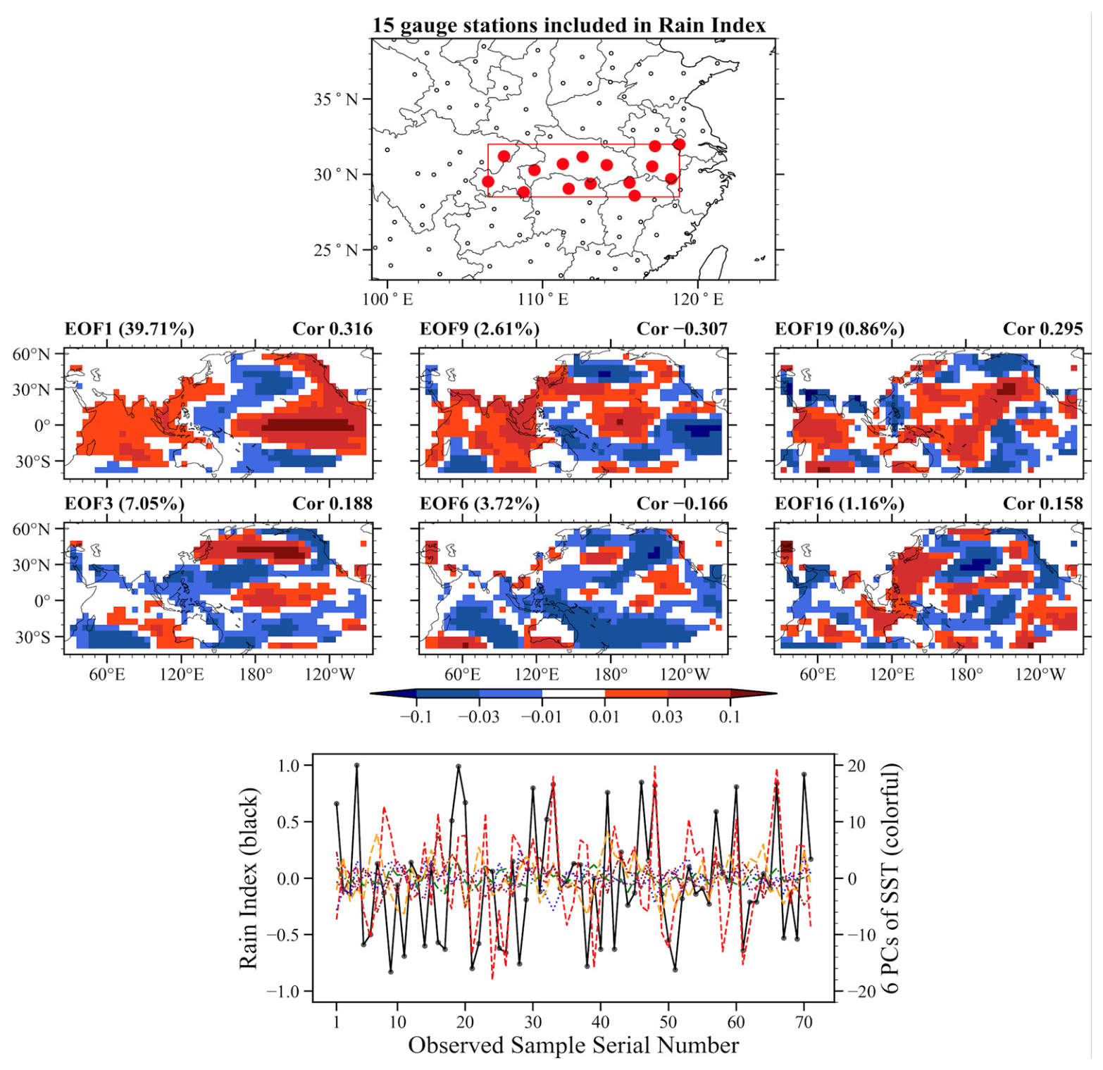
Figure A1 shows the 15 stations in the MLYR region. Among these stations, the composite maps of prophase SST for years with high and low precipitation anomalies exhibit good similarity. Years with precipitation anomaly percentages exceeding ±25% are defined as abnormal years. The precipitation anomaly percentages for abnormal years are amplified by 25% (e.g., 40% becomes 65% and −30% becomes −55%). This increases their contribution in establishing the prediction model, thereby strengthening the model’s capacity to predict abnormal events. The EOF analysis is first performed on the winter SST anomalies from 1951 to 2021 to derive the 30 leading eigenvectors. The 30 PCs are then calculated by projecting the SST anomalies onto these EOF eigenvectors. Note that the perturbation magnitudes vary across different PCs, and normalization is not used. Those 30 PCs are ranked in descending order of their correlation with Rain.
Figure A1 shows the six EOF modes used for calculating SST predictor variables (i.e., PCs) and the specific data of the observed samples.
Figure A1.
The rain gauge stations (red dots) used for calculating the Rain Index (upper panel), the six EOF eigenvectors corresponding to the six SST PCs (default setting) that serve as predictor variables (middle panel), and the observed samples (one Rain Index and six SST PCs) used for the NN model (lower panel). The EOF mode number and its variance contribution are shown at the upper-left corner, and the linear correlation coefficient (Cor) between the corresponding PC and Rain is shown at the upper-right corner. For the observed samples, the Rain Index is plotted as a black line (left Y-axis), while the six SST PCs are plotted as colorful lines (right Y-axis).
Figure A1.
The rain gauge stations (red dots) used for calculating the Rain Index (upper panel), the six EOF eigenvectors corresponding to the six SST PCs (default setting) that serve as predictor variables (middle panel), and the observed samples (one Rain Index and six SST PCs) used for the NN model (lower panel). The EOF mode number and its variance contribution are shown at the upper-left corner, and the linear correlation coefficient (Cor) between the corresponding PC and Rain is shown at the upper-right corner. For the observed samples, the Rain Index is plotted as a black line (left Y-axis), while the six SST PCs are plotted as colorful lines (right Y-axis).
References
- Liu, Y.; Ren, H.; Zhang, P.; Zuo, J.; Tian, B.; Wan, J.; Li, Y. Application of the Hybrid Statistical Downscaling Model in Summer Precipitation Prediction in China. Clim. Environ. Res. 2020, 25, 163–171. (In Chinese) [Google Scholar]
- Troccoli, A. Seasonal Climate Forecasting. Meteorol. Appl. 2010, 17, 251–268. [Google Scholar] [CrossRef]
- Xing, W.; Wang, B.; Yim, S. Long-lead seasonal prediction of China summer rainfall using an EOF–PLS regression-based methodology. J. Clim. 2016, 29, 1783–1796. [Google Scholar] [CrossRef]
- Wang, T.; Huang, P. Superiority of a Convolutional Neural Network Model over Dynamical Models in Predicting Central Pacific ENSO. Adv. Atmos. Sci. 2024, 41, 141–154. [Google Scholar] [CrossRef]
- Mekanik, F.; Imteaz, M.A.; Gato-Trinidad, S.; Elmahdi, A. Multiple Regression and Artificial Neural Network for Long-Term Rainfall Forecasting Using Large Scale Climate Modes. J. Hydrol. 2013, 503, 11–21. [Google Scholar] [CrossRef]
- Anirudh, K.M.; Raj, P.; Sandeep, S.; Kodamana, H.; Sabeerali, C.T. A Skillful Prediction of Monsoon Intraseasonal Oscillation Using Deep Learning. J. Geophys. Res. Mach. Learn. Comput. 2025, 2, e2024JH000504. [Google Scholar] [CrossRef]
- Bommer, P.L.; Kretschmer, M.; Spuler, F.R.; Bykov, K.; Höhne, M.M.-C. Deep Learning Meets Teleconnections: Improving S2S Predictions for European Winter Weather. Mach. Learn. Earth 2025, 1, 015002. [Google Scholar] [CrossRef]
- Yang, S.; Ling, F.; Ying, W.; Yang, S.; Luo, J. A Brief Overview of the Application of Artificial Intelligence to Climate Prediction. Trans. Atmos. Sci. 2022, 45, 641. (In Chinese) [Google Scholar] [CrossRef]
- Wang, G.-G.; Cheng, H.; Zhang, Y.; Yu, H. ENSO Analysis and Prediction Using Deep Learning: A Review. Neurocomputing 2023, 520, 216–229. [Google Scholar] [CrossRef]
- Materia, S.; García, L.P.; van Straaten, C.; O, S.; Mamalakis, A.; Cavicchia, L.; Coumou, D.; de Luca, P.; Kretschmer, M.; Donat, M. Artificial Intelligence for Climate Prediction of Extremes: State of the Art, Challenges, and Future Perspectives. WIREs Clim. Change 2024, 15, e914. [Google Scholar] [CrossRef]
- Ham, Y.-G.; Kim, J.-H.; Luo, J.-J. Deep Learning for Multi-Year ENSO Forecasts. Nature 2019, 573, 568–572. [Google Scholar] [CrossRef]
- Gibson, P.B.; Chapman, W.E.; Altinok, A.; Delle Monache, L.; DeFlorio, M.J.; Waliser, D.E. Training Machine Learning Models on Climate Model Output Yields Skillful Interpretable Seasonal Precipitation Forecasts. Commun. Earth Environ. 2021, 2, 159. [Google Scholar] [CrossRef]
- Yang, S.; Ling, F.; Li, Y.; Luo, J.-J. Improving Seasonal Prediction of Summer Precipitation in the Middle–Lower Reaches of the Yangtze River Using a TU-Net Deep Learning Approach. Artif. Intell. Earth Syst. 2023, 2, 220078. [Google Scholar] [CrossRef]
- Hoffman, L.; Massonnet, F.; Sticker, A. Probabilistic Forecasts of September Arctic Sea Ice Extent at the Interannual Timescale With Data-Driven Statistical Models. J. Geophys. Res. Mach. Learn. Comput. 2025, 2, e2025JH000669. [Google Scholar] [CrossRef]
- Tangang, F.T.; Hsieh, W.W.; Tang, B. Forecasting the Equatorial Pacific Sea Surface Temperatures by Neural Network Models. Clim. Dyn. 1997, 13, 135–147. [Google Scholar] [CrossRef]
- Wu, A.; Hsieh, W.W.; Tang, B. Neural Network Forecasts of the Tropical Pacific Sea Surface Temperatures. Neural Netw. 2006, 19, 145–154. [Google Scholar] [CrossRef]
- Sun, C.; Shi, X.; Yan, H.; Jiang, Q.; Zeng, Y. Forecasting the June Ridge Line of the Western Pacific Subtropical High with a Machine Learning Method. Atmosphere 2022, 13, 660. [Google Scholar] [CrossRef]
- Amir, S.; Van De Meent, J.-W.; Wallace, B. On the Impact of Random Seeds on the Fairness of Clinical Classifiers. In Proceedings of the 2021 Conference of the North American Chapter of the Association for Computational Linguistics: Human Language Technologies, Online, 6–11 June 2021. [Google Scholar]
- Gundersen, O.E.; Coakley, K.; Kirkpatrick, C.; Gil, Y. Sources of Irreproducibility in Machine Learning: A Review. arXiv 2023, arXiv:2204.07610. [Google Scholar] [CrossRef]
- Zhang, T.; Wu, F.; Katiyar, A.; Weinberger, K.Q.; Artzi, Y. Revisiting Few-Sample BERT Fine-Tuning. arXiv 2021, arXiv:2006.05987. [Google Scholar] [CrossRef]
- Keshari, R.; Ghosh, S.; Chhabra, S.; Vatsa, M.; Singh, R. Unravelling Small Sample Size Problems in the Deep Learning World. In Proceedings of the 2020 IEEE Sixth International Conference on Multimedia Big Data (BigMM), New Delhi, India, 24–26 September 2020. [Google Scholar] [CrossRef]
- Pecher, B.; Srba, I.; Bielikova, M. A Survey on Stability of Learning with Limited Labelled Data and Its Sensitivity to the Effects of Randomness. ACM Comput. Surv. 2025, 57, 1–40. [Google Scholar] [CrossRef]
- Jiang, Q.; Shi, X. Forecasting the July Precipitation over the Middle-Lower Reaches of the Yangtze River with a Flexible Statistical Model. Atmosphere 2023, 14, 152. [Google Scholar] [CrossRef]
- Kaplan, A.; Cane, M.A.; Kushnir, Y.; Clement, A.C.; Blumenthal, M.B.; Rajagopalan, B. Analyses of Global Sea Surface Temperature 1856–1991. J. Geophys. Res. Ocean. 1998, 103, 18567–18589. [Google Scholar] [CrossRef]
- Fan, K.; Wang, H.; Choi, Y.-J. A Physically-Based Statistical Forecast Model for the Middle-Lower Reaches of the Yangtze River Valley Summer Rainfall. Chin. Sci. Bull. 2008, 53, 602–609. [Google Scholar] [CrossRef]
- Huang, P.; Huang, R.-H. Relationship between the Modes of Winter Tropical Pacific SST Anomalies and the Intraseasonal Variations of the Following Summer Rainfall Anomalies in China. Atmos. Ocean. Sci. Lett. 2009, 2, 295–300. [Google Scholar] [CrossRef]
- Cai, Y.; Shi, X. A Comparative Study on the Methods of Predictor Extraction from Global Sea Surface Temperature Fields for Statistical Climate Forecast System. Atmosphere 2025, 16, 349. [Google Scholar] [CrossRef]
- Patel, P.; Nandu, M.; Raut, P. Initialization of Weights in Neural Networks. Int. J. Sci. Dev. Res. 2018, 3, 73–79. [Google Scholar]
- Kingma, D.P.; Ba, J. Adam: A Method for Stochastic Optimization. arXiv 2014, arXiv:1412.6980. [Google Scholar] [CrossRef]
- Mahsereci, M.; Balles, L.; Lassner, C.; Hennig, P. Early Stopping without a Validation Set. arXiv 2017, arXiv:1703.09580. [Google Scholar] [CrossRef]
- Hansen, L.K.; Salamon, P. Neural network ensembles. IEEE Trans. Pattern Anal. Mach. Intell. 1990, 12, 993–1001. [Google Scholar] [CrossRef]
- Krogh, A.; Vedelsby, J. Neural network ensembles, cross validation, and active learning. In Advances in Neural Information Processing Systems 7; Tesauro, G., Touretzky, D.S., Leen, T.K., Eds.; MIT Press: Cambridge, MA, USA, 1995; pp. 231–238. Available online: https://dL.acm.org/doi/abs/10.5555/2998687.2998716 (accessed on 15 May 2026).
- Gundersen, O.E.; Shamsaliei, S.; Kjærnli, H.S.; Langseth, H. On Reporting Robust and Trustworthy Conclusions from Model Comparison Studies Involving Neural Networks and Randomness. In Proceedings of the 2023 ACM Conference on Reproducibility and Replicability, Santa Cruz, CA, USA, 27–29 June 2023. [Google Scholar] [CrossRef]
- Sheng, Z.; Xie, S.; Pan, C. Probability and Mathematical Statistics; Higher Education Press: Beijing, China, 2008; pp. 30–54. (In Chinese) [Google Scholar]
- Krogh, A.; Hertz, J. A Simple Weight Decay Can Improve Generalization. In Advances in Neural Information Processing Systems 4; Moody, J.E., Hanson, S.J., Lippmann, R.P., Eds.; Morgan Kaufmann: San Mateo, CA, USA, 1992; pp. 950–957. [Google Scholar]
- Smith, L.N. A Disciplined Approach to Neural Network Hyper-Parameters: Part 1—Learning Rate, Batch Size, Momentum, and Weight Decay. arXiv 2018, arXiv:1803.09820. [Google Scholar] [CrossRef]
| Disclaimer/Publisher’s Note: The statements, opinions and data contained in all publications are solely those of the individual author(s) and contributor(s) and not of MDPI and/or the editor(s). MDPI and/or the editor(s) disclaim responsibility for any injury to people or property resulting from any ideas, methods, instructions or products referred to in the content. |