Comparison of Simple Temporal and Climatological Baselines, Deterministic Spatial Interpolation, and Hybrid Machine-Learning Methods for Imputing Precipitation Data Using ERA5-Land Climate Data

Abstract

Precipitation records from meteorological stations frequently contain gaps caused by sensor, power, or transmission failures, creating uncertainty in hydrological, agricultural, and water-resources applications. This study compared two simple baselines (station-specific monthly climatological mean and temporal linear interpolation), deterministic spatial interpolation, direct reanalysis-based replacement, and machine-learning methods for daily precipitation imputation. Daily precipitation from 14 stations in Eastern and Southeastern Türkiye during 1985–2014 was evaluated using an independent final-test set formed by stratified random masking of 15% of complete observations; the remaining 85% was used for calibration, SHapley Additive exPlanations (SHAP) analysis, cross-validation, and hyperparameter optimization. ERA5-Land variables were transferred to the stations, precipitation was calibrated by Empirical Quantile Mapping, and leakage-controlled Kriging estimates were incorporated as predictors in XGBoost, LightGBM, Random Forest, Support Vector Regression, and Multilayer Perceptron models. The station-month climatological mean (RMSE = 5.4820 mm; NSE = 0.0527) and temporal linear interpolation (RMSE = 5.7059 mm; NSE = −0.0262) performed substantially worse than optimized Kriging and IDW. The full-hybrid LightGBM model achieved the best performance (RMSE = 3.2001 mm; MAE = 0.9814 mm; Pearson r = 0.8317; NSE = 0.6772), whereas direct ERA5-EQM replacement was less accurate (RMSE = 5.2252 mm; NSE = 0.1394). Combining local observations, spatial information, and ERA5-Land covariates therefore improved daily precipitation imputation in the study region.

1. Introduction

Meteorological observation networks play a critical role as fundamental data sources in many areas, such as monitoring the effects of climate change, water resources management, agricultural planning, and disaster risk assessment [1,2]. However, the problem of missing data frequently arises as a common challenge due to technical issues like automatic meteorological observation station device failures and power outages. Precipitation measurement stations operated by the Turkish State Meteorological Service (MGM) in Türkiye are also affected by these problems, and missing data threaten the reliability of analyses, particularly in long-term data series. Imputing missing data is an indispensable necessity to ensure data continuity and improve accuracy in hydrometeorological modelling [3].

Reanalysis datasets provide spatially and temporally complete meteorological fields that can support missing-data reconstruction [4]. ERA5-Land supplies precipitation, temperature, dew-point temperature, pressure, and related land-surface variables at regular spatial and temporal intervals [5,6]. However, its precipitation represents a grid-cell estimate rather than a point-gauge measurement and may smooth or displace localized rainfall. ERA5-Land precipitation was therefore evaluated both after bias correction and as an auxiliary covariate in the hybrid models.

Simple station-internal methods provide transparent and inexpensive benchmarks. Temporal linear interpolation estimates a missing value from the nearest valid observations before and after the target date, whereas a station-specific monthly climatological mean uses the development-period mean for the same station and calendar month [7,8]. Because daily precipitation is intermittent and event-driven, these methods may not reproduce rainfall occurrence or magnitude. IDW and Kriging provide physically interpretable spatial benchmarks based on neighbouring gauges and, for Kriging, the variogram structure [9,10,11].

Recent precipitation-imputation studies have combined neighbouring-gauge information with machine-learning models. Some studies have separated rain/no-rain classification from rainfall-amount regression in large sensor networks [12], reconstructed rainfall series affected by missing or anomalous observations [13], and compared data-driven and spatial imputation methods [14]. These studies show that performance depends on precipitation intermittency, station density, topography, auxiliary information, and validation design.

The five model families used here represent complementary nonlinear learning mechanisms. XGBoost and LightGBM provide regularized gradient boosting [15,16], Random Forest uses bagged decision trees [17], MLP represents nonlinear neural regression [18], and radial-basis-function SVR provides kernel regression [19,20]. Similar model families have been used with neighbouring gauges and gridded precipitation information in precipitation-recovery and merging studies [12,13,21].

Hybridization is especially relevant when no single data source fully describes the target process. Neighbouring-gauge precipitation conveys the same-day spatial structure of rainfall; lagged target-station observations describe short-term temporal persistence; seasonal sine and cosine terms represent the annual cycle; ERA5-Land temperature, dew-point temperature, pressure, and derived relative humidity describe the broader atmospheric moisture state; and calibrated ERA5-Land precipitation provides a spatially continuous precipitation signal. A leave-one-out Kriging estimate can further summarize spatial dependence without directly supplying the target observation itself. Machine-learning models can then learn when each source is informative and when it should be down-weighted. This architecture differs from using Kriging or ERA5-Land as a final replacement: the spatial and reanalysis estimates are treated as predictors whose contribution is evaluated jointly with the remaining covariates. Model interpretability was assessed using SHapley Additive exPlanations (SHAP), an additive feature-attribution framework grounded in cooperative game theory that assigns each predictor a contribution value for an individual model prediction [22].

A leakage-controlled design is essential because calibration, predictor generation, feature interpretation, variogram selection, and hyperparameter tuning can otherwise use information from observations later reported as test cases. This study therefore compared simple station-internal baselines, deterministic spatial interpolation, direct ERA5-Land correction, and hybrid machine-learning models using a common independent test set. The analysis quantified the incremental contribution of same-day spatial information, ERA5-Land covariates, and nonlinear learning.

2. Materials and Methods

2.1. Study Area

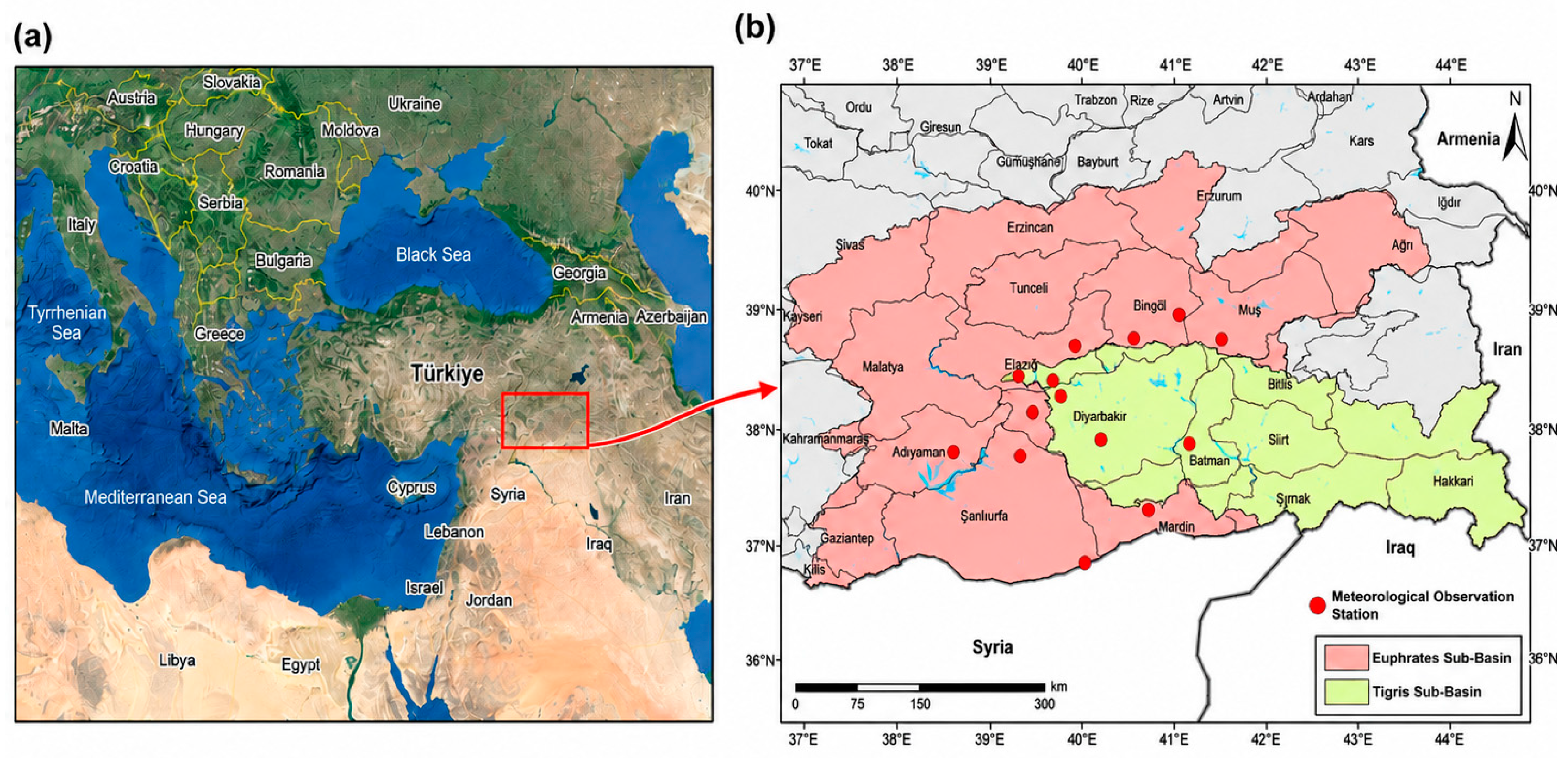
The study area is located between 36° and 40° North latitudes and 38° and 42° East longitudes, covering Türkiye’s Eastern Anatolia and Southeastern Anatolia regions, as well as the Euphrates-Tigris basin, including the central province of Diyarbakır and neighbouring provinces with adjacent stations. The approximate surface area of the study region is 30,000 km², all of which lies within the Euphrates-Tigris basin [23]. The study area, centred on Diyarbakır Province in southeastern Türkiye, is presented in Figure 1.

The study area centred on Diyarbakır Province has a continental climate characterized by hot, dry summers and cold winters. According to the official long-term meteorological statistics for Diyarbakır covering the 1929–2025 observation period, the annual mean temperature is approximately 16.0 °C, while the recorded maximum and minimum temperatures are 46.2 °C and −24.2 °C, respectively. The mean annual precipitation is approximately 487 mm, with precipitation concentrated mainly during winter and spring and very low amounts occurring during the summer months [24].

2.2. Datasets

2.2.1. Observed Dataset

Thirty years of daily total precipitation data from 1985 to 2014 for 14 meteorological observation stations were obtained from the Turkish State Meteorological Service. The precipitation data were expressed in millimetres (mm). The selected period includes 10,957 daily records for each station, corresponding to a total expected number of 153,398 station-day precipitation observations across the 14 stations.

Station selection was based on coverage of the common 1985–2014 reference period rather than on the total number of stations currently operating in the broader region. Some stations in and around the study area had operated only for short periods and were subsequently closed, whereas several additional stations were commissioned mainly during 2013–2015. Because these records did not provide adequate coverage of the common 30-year period, they were excluded. The 14 retained stations were therefore the stations within or adjacent to the study domain that provided daily precipitation series spanning the common reference period; their remaining missing records are summarized in

Table 1. Meteorological stations and missing-data summary.

No.	Station	Latitude (°N)	Longitude (°E)	Elevation (m)	Expected Records (n)	Missing Records (n)	Missing (%)
1	MUŞ/17204	38.7509	41.5023	1322	10,957	11	0.10
2	MARDİN/17275	37.3103	40.7284	1040	10,957	0	0.00
3	DİYARBAKIR HAVALİMANI/17280	37.8973	40.2027	674	10,957	0	0.00
4	BATMAN/17282	37.8636	41.1562	610	10,957	95	0.87
5	SOLHAN/17776	38.9597	41.0503	1366	10,957	81	0.74
6	PALU/17806	38.6907	39.9260	869	10,957	0	0.00
7	GENÇ/17808	38.7616	40.5577	993	10,957	4	0.04
8	SİVRİCE/17844	38.4507	39.3101	1240	10,957	19	0.17
9	MADEN/17846	38.3924	39.6757	1047	10,957	33	0.30
10	ERGANİ/17847	38.2670	39.7660	986	10,957	85	0.78
11	ÇERMİK/17874	38.1371	39.4644	695	10,957	0	0.00
12	KAHTA/17910	37.7918	38.6155	725	10,957	525	4.79
13	SİVEREK/17912	37.7522	39.3291	801	10,957	13	0.12
14	CEYLANPINAR TİGEM/17968	36.8406	40.0307	360	10,957	10	0.09
Total	—	—	—	—	153,398	876	0.57

.

Before model development, the completeness of the observed precipitation dataset was examined at station level. A total of 876 missing daily precipitation records were identified, corresponding to an overall missing-data ratio of 0.57%. The missing-data percentage varied among stations, with most stations having very low missing ratios. The highest missing-data ratio was observed at Kahta station, with 525 missing records corresponding to 4.79% of its expected daily precipitation series. The station locations, elevations, expected number of daily precipitation records, missing precipitation counts, and missing-data percentages are presented in Table 1.

Because the reference period of the CMIP6 global climate models used in climate change studies ends in 2014, and since 30-year climate datasets are commonly employed in climatological research, the period between 1985 and 2014 was selected for the completion of missing precipitation data.

2.2.2. ERA5-Land Climate Data

The reanalysis product used in this study was the ERA5-Land hourly dataset rather than the atmospheric ERA5 product. ERA5-Land is generated by replaying the land component of the ERA5 reanalysis using atmospheric forcing from ERA5 [5,6]. It has an approximate native horizontal resolution of 9 km and is distributed by the Copernicus Climate Data Store on a regular 0.1° × 0.1° latitude–longitude grid at hourly temporal resolution [6]. Hourly total precipitation, 2 m air temperature, 2 m dew-point temperature, and surface pressure were obtained for the 1985–2014 period and the spatial domain bounded by 36–40° N and 38–42° E. Hourly precipitation was aggregated to daily totals, whereas air temperature, dew-point temperature, and surface pressure were aggregated to daily means. Precipitation was converted to millimetres, air and dew-point temperatures to degrees Celsius, and surface pressure to hectopascals.

The regular 0.1° ERA5-Land grid was retained because it is finer than the irregular 14-station network and provides complete meteorological fields over the study area and reference period. Because a grid-cell value is not equivalent to a point-gauge observation, the four surrounding ERA5-Land cells were transferred to each station by IDW in UTM Zone 37N, as detailed in Section 2.3.4. This procedure interpolated the existing gridded field to station locations without implying additional sub-grid observations.

ERA5 variables contain useful large-scale atmospheric information when integrated with local station observations and spatial interpolation features. Therefore, ERA5 should be interpreted as a valuable auxiliary data source rather than a direct substitute for ground-based precipitation measurements.

2.3. Method

The computational experiment used a common leakage-controlled framework to compare simple baselines, direct ERA5-EQM replacement, deterministic spatial interpolation, and three machine-learning scenarios. Fifteen percent of complete station-day observations were reserved as an independent final-test set, and all calibration, predictor generation, SHAP analysis, cross-validation, and parameter selection were restricted to the remaining 85% development pool.

The development pool was evaluated by five-fold shuffled stratified cross-validation at the individual station-day level. Validation targets were masked before precipitation-dependent predictors were generated; dates and stations were not used as grouping units. The precipitation-intensity strata and model-selection rule are defined in Section 2.3.14.

The predictor groups and their scientific roles are described in Section 2.3.5. SHAP was used to interpret the fitted full-hybrid LightGBM model rather than to eliminate predictors; all 17 predefined predictors were retained for the full-hybrid analysis.

Hybridization was implemented at the predictor level. For each target station-day, the target observation was masked and a same-day leave-one-out ordinary Kriging estimate was generated from the remaining stations and added as kriging_feature. The final estimate was produced by the two-stage machine-learning model; Kriging and machine-learning outputs were not averaged. Basic machine learning used temporal, neighbouring-gauge, and station-context predictors; the Kriging-supported scenario added kriging_feature; and the full-hybrid scenario additionally included EQM-corrected ERA5-Land precipitation and meteorological covariates. All scenarios used the same data partitions, algorithms, and evaluation metrics.

Data analysis was performed using Python version 3.13.7.

2.3.1. Data Control

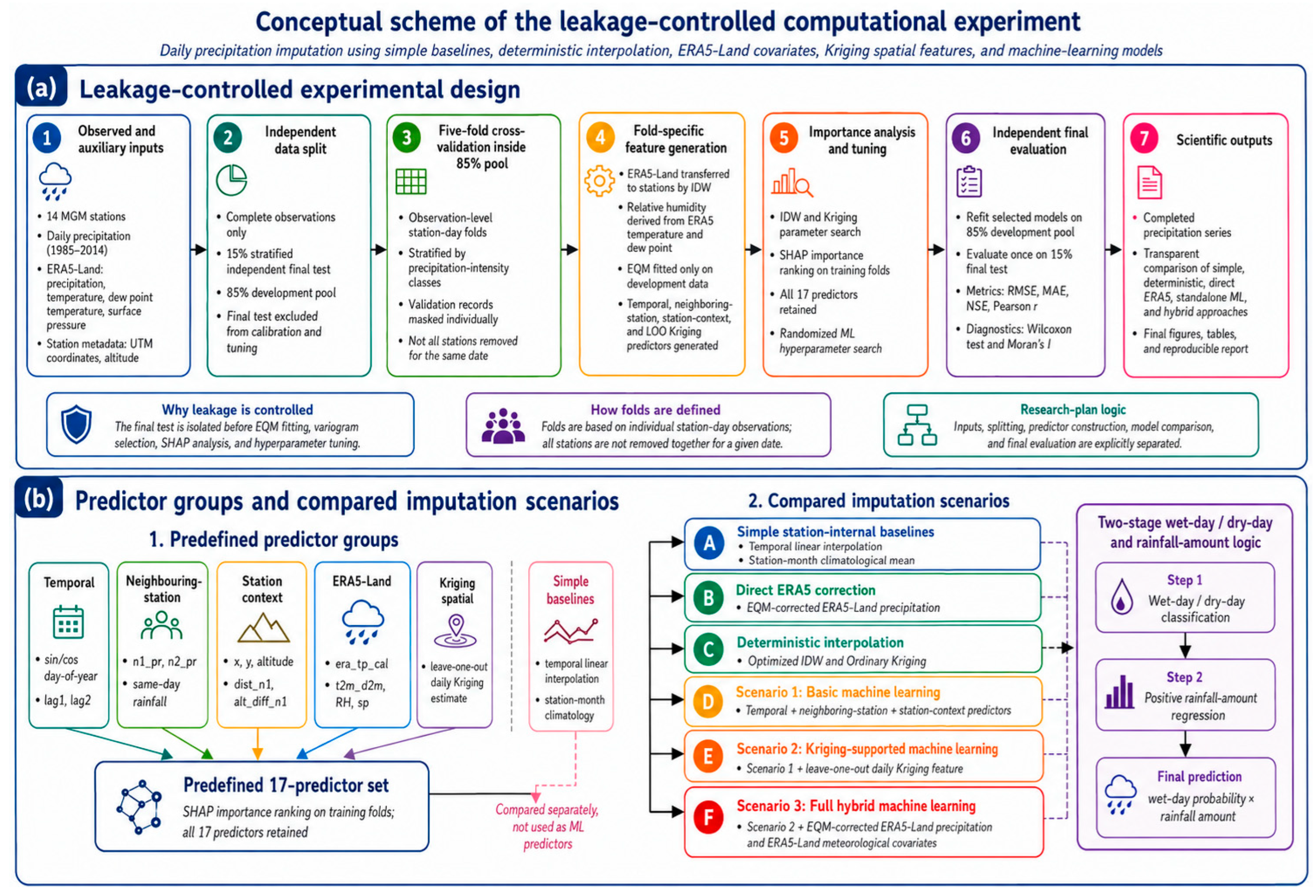
For the proper planning and management of water resources, precipitation data collected by meteorological observation stations must be consistent and complete [8,25]. Precipitation data must be 0 or positive values; they cannot be negative [26]. Before imputing missing precipitation data, it is crucial to verify the data to select the right methods and ensure better model performance. In this study, the location, status, number, and any missing or incorrect values of the 14 stations’ data were checked manually and via software. The checks revealed that the distance between stations was variable, with some exceeding 100 km, indicating a sparse station network. There were no negatively signed precipitation values, and since the stations are in a semi-arid region, zero-value precipitation events were frequent. The leakage-controlled experimental workflow and the compared precipitation-imputation scenarios are summarized in Figure 2.

2.3.2. Calculating Relative Humidity from ERA5-Land Data

Relative humidity represents atmospheric moisture conditions and may provide useful auxiliary information for precipitation estimation. However, ERA5 reanalysis climate data do not directly contain relative humidity. It must be generated through calculation. Since ERA5 reanalysis relative humidity (RH) data are not directly provided, they were calculated using temperature (T) and dew point temperature (Td) variables based on the updated Magnus formulation by Alduchov & Eskridge (1996) [27]. This method is considered one of the most accurate and widely accepted approaches in the literature. This method, which is routinely employed by the NOAA and the ECMWF, is widely recognized in the literature as one of the most common and reliable approaches [5,28]. Since ERA5 does not directly provide relative humidity in the downloaded variables, daily mean relative humidity was derived from 2 m air temperature and 2 m dew point temperature using the Magnus-type saturation vapor pressure formulation. ERA5 temperature variables were first converted from Kelvin to degrees Celsius using Equations (1) and (2):

$${\mathrm{T}}_{°\mathrm{C}}={\mathrm{T}}_{\mathrm{K}}-273.15$$

(1)

$${\mathrm{T}}_{\mathrm{d},°\mathrm{C}}={\mathrm{T}}_{\mathrm{d},\mathrm{K}}-273.15$$

(2)

The saturation vapor pressure at temperature $T$ was computed as Equation (3):

$${\mathrm{e}}_{\mathrm{s}}\left(\mathrm{T}\right)=6.112\times \mathrm{e}\mathrm{x}\mathrm{p}\left({\displaystyle \frac{17.67\mathrm{T}}{\mathrm{T}+243.5}}\right)$$

(3)

Relative humidity was then calculated as Equation (4):

$$RH\left(\%\right)=100\times {\displaystyle \frac{e_s\left(T_d\right)}{e_s\left(T\right)}}$$

(4)

where $T$ is air temperature in °C, $T_d$ is dew point temperature in °C, $e_s\left(T\right)$ and $e_s\left(T_d\right)$ are the saturation vapor pressures in hPa, and $RH$ is the relative humidity expressed as a percentage. Values were constrained to the physically meaningful interval of 0–100%.

2.3.3. Simple Temporal and Statistical Baselines

To test whether the target-station time series alone was sufficient, two low-complexity reference methods were evaluated on exactly the same 22,878 independent final-test records as the spatial and machine-learning approaches: temporal linear interpolation and the station-specific monthly climatological mean. Before either baseline was calculated, all final-test precipitation values were masked simultaneously and the 876 naturally missing records remained unavailable. Thus, no withheld precipitation value contributed to another prediction or to the climatological statistics. Neither baseline required hyperparameter tuning [7,8].

For a target record at station s and date t, temporal linear interpolation used the nearest earlier and later non-test precipitation observations at the same station, occurring at t1 and t2, respectively. The estimate was calculated as follows:

$$\widehat{P}(\mathrm{s},\mathrm{t})=P(\mathrm{s},t_1)+{\displaystyle \frac{t-t_1}{t_2-t_1}}[P(\mathrm{s},t_2)-P(\mathrm{s},t_1)]$$

(5)

Both bracketing observations were available for 22,869 of the 22,878 final-test records. For the nine boundary records lacking a valid observation on one side of the target date, the station-specific monthly climatological mean defined below was used as a fallback. No test record was removed from metric calculation.

The station-specific monthly climatological mean assigned each target record the arithmetic mean of all development-pool precipitation observations from the same station s and calendar month m:

$$\widehat{P}(\mathrm{s},\mathrm{m})={\displaystyle \frac{1}{N(\mathrm{s},\mathrm{m})}}\sum P(\mathrm{s},\mathrm{d})$$

(6)

where Ddev denotes the development pool, and N(s,m) is the number of available development observations for station s in month m. This baseline represents broad station-specific seasonality but contains no event-specific neighbouring-station, reanalysis, or geostatistical information.

2.3.4. Inverse Distance Weighting for ERA5-Land Transfer and Station-Based Gap Filling

Inverse Distance Weighting (IDW) was used in two distinct operations, both following the distance-decaying weighting expression in Equation (7) [9]. First, the daily ERA5-Land variables were transferred from the regular grid to each meteorological station using the four nearest grid-cell centres. Euclidean distances were calculated in WGS84/UTM Zone 37N, the distance exponent was fixed at p = 2, and no fixed search radius was imposed because the four nearest grid cells were always available on the regular ERA5-Land grid.

Mathematically, the unknown value of Z(x_0) is shown in Equation (7):

$$Z(x_0)={\displaystyle \frac{{\displaystyle {\sum }_{\mathrm{i}=1}^{\mathrm{N}}}\frac{\mathrm{Z}\left({\mathrm{x}}_{\mathrm{i}}\right)}{\mathrm{d}{({\mathrm{x}}_0,{\mathrm{x}}_{\mathrm{i}})}^{\mathrm{p}}}}{{\displaystyle {\sum }_{\mathrm{i}=1}^{\mathrm{N}}}\frac{1}{\mathrm{d}{({\mathrm{x}}_0,{\mathrm{x}}_{\mathrm{i}})}^{\mathrm{p}}}}}$$

(7)

where denotes the interpolated value at the target location, represents the observed values at neighbouring points, is the distance between the unknown and known points, is the distance weighting exponent, and is the number of observation points.

For the independent station-to-station IDW benchmark, the same equation was applied to available same-day MGM precipitation observations rather than ERA5-Land grid-cell values. The candidate distance exponents (1.5, 2.0, and 2.5), maximum neighbourhood sizes (4, 6, and 8 stations), and maximum search radii (120, 150, and 200 km) were selected entirely within the 85% development pool by five-fold cross-validation. The final configuration used p = 1.5, a maximum of eight neighbouring stations, and a 150 km search radius. If fewer than three stations were available within that radius, the three nearest available stations were used as a fallback so that an estimate could still be generated. Thus, the two IDW applications shared the same mathematical form but differed in their source points and parameter-selection rules.

2.3.5. Candidate Predictors and Their Scientific Rationale

Seventeen candidate predictors were defined a priori and grouped according to their temporal, neighbouring-station, geographic, topographic, reanalysis-based, and geostatistical roles. The temporal group consisted of the sine and cosine transformations of day of year (sin_doy and cos_doy), which represented the annual cycle, and the one- and two-day target-station precipitation lags (lag1 and lag2), which represented short-term temporal persistence. The lag variables corresponded strictly to precipitation observed at the target station at times t − 1 and t − 2; no future precipitation information was used. Within each cross-validation fold, the lag variables were regenerated after masking the validation observations so that the withheld target value could not enter its own predictor set.

The neighbouring-station group comprised same-day precipitation from the first and second nearest gauges (n1_pr and n2_pr). UTM easting and northing (x and y) were included as static station-location covariates so that the nonlinear learners could represent broad east-west and north-south geographic gradients across the station network. Geographic coordinates are one possible class of spatial covariates in machine-learning prediction, but proximity and autocorrelation are more directly represented by distance-based and geostatistical features [29]. Accordingly, the predictor set also included distance to the nearest station (dist_n1), elevation difference from the nearest station (alt_diff_n1), same-day neighbouring rainfall (n1_pr and n2_pr), and the leakage-controlled leave-one-out Kriging estimate (kriging_feature). Distances from each station to the ERA5-Land grid-cell centres were calculated separately in UTM Zone 37N and were used only to construct the four-neighbour IDW weights described in Section 2.3.4. Thus, x and y identify the station position within the regional domain; they do not encode ERA5-Land grid distance.

The ERA5-Land predictor group consisted of EQM-corrected precipitation (era_tp_cal), 2 m air temperature (era_t2m), 2 m dew-point temperature (era_d2m), derived relative humidity (era_rh), and surface pressure (era_sp). These variables were intended to represent the large-scale precipitation signal, atmospheric thermal state, absolute moisture content, proximity to saturation, and surface-pressure environment, respectively. The combination of environmental information from the target location and precipitation from surrounding gauges is consistent with machine-learning precipitation-recovery frameworks reported in the literature [12]. All 17 predictors were retained; SHAP was subsequently used to quantify their relative attribution within the fitted full-hybrid model rather than to eliminate lower-ranked variables.

2.3.6. XGBoost Method

XGBoost (eXtreme Gradient Boosting) is a scalable implementation of gradient boosting decision trees introduced by Tianqi Chen and Carlos Guestrin (2016) [15]. This method provides a powerful machine-learning approach for imputing missing daily precipitation data. XGBoost sequentially combines weak learners (typically decision trees) to minimize prediction errors while preventing overfitting through regularization techniques. The core principle of the method is to optimize the loss function using a second-order Taylor expansion. The objective function is shown in Equation (8):

$$Ob{j}^{\left(t\right)}={\sum }_{i=1}^{n}l\left(y_i,{\hat{y}}_i^{(t-1)}+f_t\left(x_i\right)\right)+\mathsf{\Omega }\left(f_t\right)$$

(8)

where $l$ is the loss function measuring prediction error, $f_t$ denotes the $t$-th tree, $y_i$ is the true value, ${\widehat{y}}_i^{\left(t−1\right)}$ is the prediction from the previous iteration, and $\mathsf{\Omega }(f_t)=\gamma T+{\displaystyle \frac{1}{2}}\lambda {\sum }_{j=1}^T{w}_j^2$ is the regularization term. Here, $T$ represents the number of leaves, $w_j$ are leaf weights, and $\gamma$ and $\lambda$ are hyperparameters. For missing precipitation imputation, XGBoost is trained using available data, and missing values are replaced with model predictions. Based on the gradient boosting framework proposed by Friedman (2001) [30], XGBoost can inherently handle missing values by automatically assigning them to optimal split directions.

2.3.7. LightGBM Method

LightGBM (Light Gradient Boosting Machine), developed by Microsoft and introduced by Ke et al. (2017) [16], is a gradient boosting framework that offers faster training and lower memory usage compared to XGBoost, making it suitable for large-scale daily precipitation datasets.

LightGBM employs a histogram-based algorithm and leaf-wise tree growth. The gain is as shown in Equation (9):

$$Gain={\displaystyle \frac{1}{2}}\left[{\displaystyle \frac{G_L^2}{H_L+\lambda }}+{\displaystyle \frac{G_R^2}{H_R+\lambda }}-{\displaystyle \frac{{\left(G_L+G_R\right)}^2}{H_L+H_R+\lambda }}\right]-\gamma$$

(9)

where $G_L,G_R$ are the gradient sums of left and right nodes, $H_L,H_R$ are the corresponding Hessian sums, and $\lambda ,\gamma$ are regularization parameters. For missing precipitation data, LightGBM constructs a regression model using available data. Missing values are handled via a “default direction,” and efficiency is improved using Gradient-based One-Side Sampling (GOSS) and Exclusive Feature Bundling (EFB) [16].

2.3.8. Random Forest (RF) Method

Random Forest (RF) is an ensemble learning method developed by Leo Breiman (2001) [17]. It operates by combining multiple decision trees through the bootstrap aggregating (bagging) technique and provides a robust approach for filling missing daily precipitation data. Each tree is trained on a randomly sampled subset of the data, while features are selected randomly at each split. The prediction is obtained as the average of all trees, as given in Equation (10):

$$\widehat{y}={\displaystyle \frac{1}{B}}{\sum }_{b=1}^B{f}_b\left(x\right)$$

(10)

where $B$ denotes the number of trees and $f_b$ represents the $b$-th tree. In this study, Random Forest was used as a supervised learning model within the proposed precipitation imputation framework. It was employed both as a candidate regression model and, in the two-stage architecture, as the classifier for estimating wet-day probability. The RF models were trained and evaluated using the same leakage-controlled development and independent final-test framework applied to the other machine-learning methods.

Recent precipitation-imputation studies have demonstrated the applicability of Random Forest under different missing-data mechanisms and missing-data rates [31]. In a separate sub-hourly rainfall study, RF was evaluated within both direct and two-step imputation frameworks; in the two-step approach, an RF classifier was used for rain/no-rain detection, followed by rainfall-depth estimation using alternative regression methods, including RF, under different neighbouring-station configurations [32]. Together, these studies support the use of RF as a flexible nonlinear model for precipitation gap filling and provide methodological support for its evaluation within the two-stage framework adopted in the present study.

2.3.9. Neural Network (MLP) Method

The Multilayer Perceptron (MLP) is a fundamental form of artificial neural networks, popularized by David E. Rumelhart et al. (1986) [33]. It is a regression-based approach capable of modelling non-linear relationships to estimate missing daily precipitation values.

An MLP consists of an input layer, one or more hidden layers, and an output layer. The forward propagation process is defined as in Equation (11):

$$a^{\left(l\right)}=\sigma \left(W^{\left(l\right)}{a}^{\left(l-1\right)}+b^{\left(l\right)}\right)$$

(11)

where $\sigma$ denotes the activation function (e.g., ReLU), while $W$ and $b$ represent the weights and biases, respectively. Training is performed using backpropagation by minimizing the Mean Squared Error (MSE) loss function. For imputation, the MLP is trained using available data, and missing values are subsequently filled using model predictions.

2.3.10. SVR Method

Support Vector Regression (SVR) is the regression variant of Support Vector Machines developed by Vladimir Vapnik (1995) [19,20]. It provides robust predictions using the $\epsilon$-insensitive loss function and is resistant to outliers in precipitation data.

SVR solves the optimization problem given in Equation (12):

$$\mathrm{m}\mathrm{i}\mathrm{n}{\displaystyle \frac{1}{2}}{\left|\left|w\right|\right|}^2+C{\sum }_{i=1}^n\left({\xi }_i+{\xi }_i^{*}\right)$$

(12)

Constraint: $\mid y_i-f(x_i)\mid \le \epsilon +{\xi }_i$

The kernel trick (e.g., Radial Basis Function, RBF: $K(x_i,x_j)=exp(-\gamma \parallel x_i-x_j{\parallel }^2)$) enables modelling of non-linear relationships. For imputation, the SVR model is trained using available data, and missing values are estimated through predictions.

2.3.11. ERA5-EQM Method

Quantile Mapping (QM), widely used in the statistical calibration of climate data, is an effective technique for correcting distributional biases in model outputs [34,35,36]. In this study, the Empirical Quantile Mapping (EQM) approach was specifically adopted. Due to the highly skewed nature of daily precipitation and its large proportion of zero values (dry days), EQM was preferred over parametric methods that force the data into theoretical distributions (e.g., Gamma or Weibull). The EQM calibration functions were derived exclusively from the 85% development dataset, while the independent 15% test dataset remained completely excluded from the calibration process. This procedure was adopted to reduce potential information leakage and to ensure an unbiased evaluation of model performance. EQM directly matches the empirical cumulative distribution functions (eCDF) of station observations and ERA5 data via linear interpolation, allowing the empirical distribution of ERA5 precipitation to be adjusted toward the station-observed distribution without assuming a parametric form. To achieve this, EQM aligns these cumulative-distribution functions as expressed in Equation (13):

$$P_{ERA5\text{-}EQM}=F_{obs}^{-1}\left(F_{ERA5}\left(P_{ERA5}\right)\right)$$

(13)

where $P_{ERA5\text{-}EQM}$ is the bias-corrected ERA5 precipitation amount, $P_{ERA5}$ is the raw ERA5 precipitation amount downscaled to the station location, $F_{ERA5}$ is the empirical cumulative distribution function of ERA5 precipitation, and $F_{obs}^{-1}$ is the inverse empirical cumulative distribution function of observed station precipitation. The EQM functions were fitted only on the development/training data, and the independent final-test observations were not used in calibration.

2.3.12. Kriging Method

Kriging is a geostatistical interpolation method formalized by Matheron [11]. It was used both as an independent deterministic method and as a spatial predictor in the hybrid framework. Station coordinates were transformed to UTM Zone 37N so that distances were expressed in metric units. The variogram family, maximum neighbourhood size, and search radius were selected within the 85% development pool by five-fold cross-validation. Candidate variogram families were spherical, exponential, and Gaussian; candidate search radii were 120, 150, and 200 km; and candidate maximum neighbourhood sizes were 4, 6, and 8 stations.

The Kriging procedure was purely spatial and was repeated independently for each target station-day; no temporal lag or spatiotemporal covariance term was included. For the standalone Kriging benchmark, the exponential variogram family, a maximum neighbourhood of eight stations, and a 120 km search radius were selected by five-fold cross-validation within the 85% development dataset. A single regional nugget, sill, or range was not imposed across all predictions. Because variogram parameters were not supplied explicitly to PyKrige, they were estimated adaptively from the available same-day local neighbouring observations for each Kriging fit. Zero precipitation values were retained as valid observations. If the selected values were effectively constant, including an all-zero neighbourhood, their mean was returned; if fewer than three usable neighbours were available or the Kriging fit failed, the corresponding IDW estimate was used. Negative Kriging estimates were constrained to zero. Thus, the procedure represents target-specific local spatial Kriging, whereas wet-day occurrence and positive rainfall amount were handled separately by the two-stage machine-learning framework.

The Ordinary Kriging estimator is expressed in Equation (14):

$$\hat{Z}(x_0)={\displaystyle {\sum }_{i=1}^n}{\lambda }_{i}Z(x_i),\sum {\lambda }_i=1{\lambda }_i\gamma (h)$$

(14)

The weights are determined using the semivariogram, defined in Equation (15):

$$\gamma (h)={\displaystyle \frac{1}{2}}E[{(Z(x)-Z(x+h))}^2]$$

(15)

where is the estimated value at the unknown location, are observed values at known locations, are weighting coefficients, is the number of neighbouring observations, is the distance between two points, is the semivariogram (a measure of spatial dependence), and denotes the expectation operator. Missing values are interpolated using neighbouring observations.

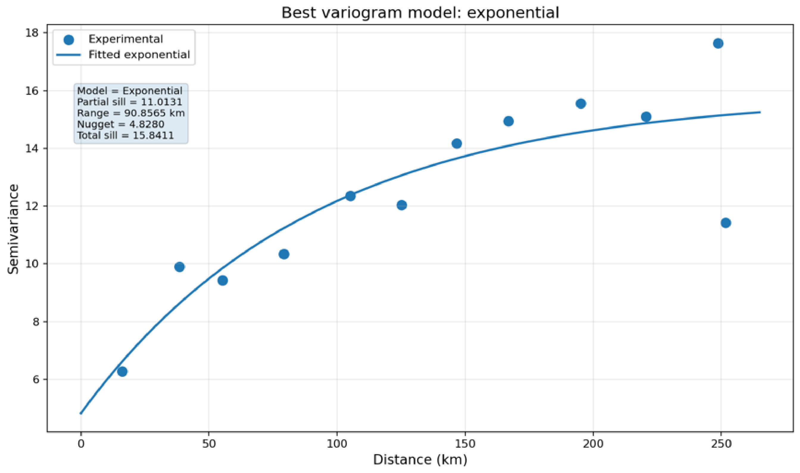
A pooled same-day empirical semivariogram was calculated by grouping semivariances from station pairs observed on the same date into 12 distance classes across the study period. The fitted curve was used only as a descriptive summary; local Kriging predictions used the cross-validated exponential family with adaptively fitted parameters.

2.3.13. Two-Stage Wet-Day Probability and Rainfall Amount Modelling

Because daily precipitation data are zero-inflated and highly right-skewed, the machine-learning framework was implemented as a two-stage architecture. In the first stage, a Random Forest classifier estimated the probability of a wet day using the retained predictors. In the second stage, the positive rainfall amount was estimated using the optimized regression model. The regression target was transformed using log1p, defined as log1p(y) = ln(1 + y), where y is precipitation in millimetres. This transformation is defined at y = 0 and compresses large positive values, thereby reducing right skewness and stabilizing model fitting. Predicted values were returned to the original precipitation scale using the inverse function expm1(z) = exp(z) − 1. The final precipitation estimate was obtained by multiplying the predicted wet-day probability by the inverse-transformed positive rainfall amount. This structure reduced the tendency of regression models to convert dry days into artificial low-intensity rainfall and improved the physical consistency of the imputed series.

The final two-stage estimate can be written as in Equation (16):

$${\widehat{P}}_i=\mathrm{P}\mathrm{r}\left(W_i=1\mid {\mathbf{x}}_i\right)\times \mathrm{m}\mathrm{a}\mathrm{x}\left[0,\mathrm{e}\mathrm{x}\mathrm{p}\left({\widehat{z}}_i\right)-1\right]$$

(16)

where ${\widehat{P}}_i$ is the final estimated precipitation amount in mm, $\mathrm{P}\mathrm{r}\left(W_i=1\mid {\mathbf{x}}_i\right)$ is the predicted wet-day probability for the predictor vector ${\mathbf{x}}_i$, and ${\widehat{z}}_i$ is the model prediction in the log-transformed precipitation space.

2.3.14. Testing Method

An artificial missing-data experiment was used for controlled evaluation. Complete station-day records were assigned to five precipitation-intensity strata: dry days (≤0.1 mm) and four wet-day classes defined by quartiles of positive precipitation. The strata contained 116,667 dry records and 9587, 8379, 8968, and 8921 records in the four successive wet-day classes. With random seed 42, 15% of each stratum was assigned to the 22,878-record final-test set and the remaining 129,644 records formed the development pool.

The development pool was partitioned into five shuffled stratified folds at the individual station-day level. Dates were not blocked and stations were not held out as groups. In each fold, validation precipitation values were masked before lag, neighbouring-station, ERA5-EQM, and Kriging predictors were regenerated, preventing a target value from entering its own predictors while preserving same-day observations at other stations.

All IDW and Kriging grid configurations and the predefined machine-learning searches were evaluated using the same five folds. The configuration with the lowest mean validation RMSE was refitted on the complete development pool and evaluated once on the untouched final-test set.

The evaluation represents isolated or irregular station-day gaps for which contemporaneous observations at other stations may remain available. Long continuous gaps, complete-station holdouts, and network-wide outages require separate blocked validation designs.

2.3.15. Accuracy Metrics

To evaluate daily precipitation gap-filling performance objectively, four complementary metrics were used: RMSE, MAE, Pearson correlation coefficient (r), and Nash-Sutcliffe Efficiency (NSE). RMSE and MAE quantified error magnitude, Pearson r described linear covariation, and NSE assessed predictive skill relative to the observed mean.

The Root Mean Square Error (RMSE) represents the square root of the mean of squared differences between observed and estimated values. Due to the squaring mechanism, RMSE penalizes larger errors more heavily and is therefore particularly useful for identifying methods that produce substantial estimation errors in precipitation datasets. Lower RMSE values indicate better model performance, with a value of zero representing a perfect match between observed and estimated values.

The Root Mean Square Error (RMSE) was calculated as Equation (17):

$$RMSE=\sqrt{{\displaystyle \frac{1}{n}}{\displaystyle {\sum }_{i=1}^n}{\left(O_i-E_i\right)}^2}$$

(17)

The Mean Absolute Error (MAE) is defined as the average of the absolute differences between observed and predicted values. Unlike RMSE, it treats all errors equally and is less sensitive to outliers, providing a robust measure of the average magnitude of prediction errors. Lower MAE values indicate higher prediction accuracy, and a value of zero corresponds to perfect agreement between observations and estimates.

The Mean Absolute Error (MAE) was calculated as Equation (18):

$$MAE={\displaystyle \frac{1}{n}}{\displaystyle {\sum }_{i=1}^n}\left|O_i-E_i\right|$$

(18)

The Pearson correlation coefficient (r) measures the strength and direction of the linear relationship between observed and predicted precipitation. It ranges from −1 to 1, with values closer to 1 indicating stronger positive linear agreement.

The Pearson correlation coefficient (r) was calculated as Equation (19):

$$r={\displaystyle \frac{{\displaystyle {\sum }_{i=1}^n}\left(O_i-\bar{O}\right)\left(E_i-\bar{E}\right)}{\sqrt{{\displaystyle {\sum }_{i=1}^n}{\left(O_i-\bar{O}\right)}^2}\sqrt{{\displaystyle {\sum }_{i=1}^n}{\left(E_i-\bar{E}\right)}^2}}}$$

(19)

The Nash–Sutcliffe Efficiency (NSE) assesses the relative magnitude of residual variance compared to the variance of the observed data. It ranges from −∞ to 1, where a value of 1 indicates perfect agreement between observed and predicted values. Values greater than 0 indicate that the model performs better than the observed mean, whereas values below 0 suggest that the observed mean provides a better predictor than the model. Therefore, NSE is widely used to evaluate the overall predictive skill of precipitation gap-filling methods, with values approaching 1 indicating superior predictive performance.

The Nash-Sutcliffe Efficiency (NSE) was calculated as Equation (20):

$$NSE=1-{\displaystyle \frac{{\displaystyle {\sum }_{i=1}^n}{\left(O_i-E_i\right)}^2}{{\displaystyle {\sum }_{i=1}^n}{\left(O_i-\bar{O}\right)}^2}}$$

(20)

3. Results

In this study, simple temporal-statistical baselines, deterministic spatial interpolation, ERA5-based reanalysis approaches, standalone machine learning, and full-hybrid machine-learning models were evaluated for imputing missing daily total precipitation under the semi-arid continental climatic conditions of Eastern and Southeastern Anatolia. The final evaluation used the same 22,878 independent test observations for every method; these observations were excluded from all calibration, optimization, SHAP analysis, climatological-statistic calculations, and cross-validation stages.

3.1. SHAP-Based Feature-Importance Analysis

SHAP analysis was applied to the final full-hybrid LightGBM model fitted on the 85% development pool [22]. The mean absolute SHAP values were used to rank the contributions of the 17 retained predictors, as summarized in

Table 2. SHAP-based importance ranking of the 17 retained predictors in the final full-hybrid LightGBM model.

Rank	Predictor	Mean Absolute SHAP Value	Description
1	kriging_feature	0.32430	Kriging prediction feature
2	n1_pr	0.09720	Precipitation value of the first nearest station
3	n2_pr	0.04840	Precipitation value of the second nearest station
4	era_tp_cal	0.04130	ERA5-Land precipitation (EQM-corrected)
5	lag1	0.02730	1-day precipitation lag
6	era_t2m	0.01570	ERA5-Land 2 m air temperature
7	era_rh	0.01570	Derived ERA5-Land relative humidity
8	dist_n1	0.00740	Distance to the first nearest station
9	era_sp	0.00670	ERA5-Land surface pressure
10	x	0.00610	Station UTM easting
11	altitude	0.00580	Altitude (elevation)
12	era_d2m	0.00510	ERA5-Land dew-point temperature
13	alt_diff_n1	0.00390	Altitude difference with the first nearest station
14	cos_doy	0.00290	Cosine of day of year (seasonality)
15	y	0.00210	Station UTM northing
16	sin_doy	0.00170	Sine of day of year (seasonality)
17	lag2	0.00110	2-day lag precipitation value

. SHAP was used for interpretation rather than feature elimination, and the independent final-test set did not influence the ranking.

The Kriging-derived feature had the largest mean absolute SHAP value (0.3243), followed by first- and second-nearest-station precipitation and EQM-corrected ERA5-Land precipitation. The ranking indicates that station-based spatial information dominated the fitted model, while ERA5-Land precipitation supplied additional large-scale information.

3.2. Hyperparameter Optimization

The hyperparameter ranges for IDW, Kriging, and the machine-learning models were determined through preliminary manual trials involving different parameter combinations. Hyperparameter optimization was then performed exclusively within the 85% development pool using the same five cross-validation folds.

Table 3. Hyperparameter search spaces, parameter roles, and selected configurations (mean five-fold CV RMSE).

Method	Evaluated Search Space	Parameter Role/Rationale	Selected Configuration (Mean CV RMSE)
XGBoost	Trees (n_estimators): 150, 300, 500; depth (max_depth): 3, 5, 7; learning rate: 0.01, 0.05, 0.10; row fraction (subsample): 0.70, 0.90; feature fraction (colsample_bytree): 0.70, 1.00; minimum child weight: 1, 4; L2 penalty (reg_lambda): 1, 5.	Varies ensemble size, tree depth, shrinkage, sampling, child-node constraint, and L2 regularization to compare low-to-moderate complexity and limit overfitting.	300 trees; depth 7; learning rate 0.05; row 0.90; features 0.70; child weight 1; L2 1; RMSE 3.2902.
LightGBM	Trees (n_estimators): 200, 400, 600; depth (max_depth): −1, 4, 8; learning rate: 0.01, 0.05, 0.10; leaves (num_leaves): 15, 31, 63; feature fraction (colsample_bytree): 0.70, 0.90; L2 penalty (reg_lambda): 1, 5.	Varies boosting length, leaf/depth complexity, shrinkage, feature sampling, and L2 regularization.	400 trees; depth 8; learning rate 0.05; features 0.90; 63 leaves; L2 5; RMSE 3.2969.
Random Forest	Trees (n_estimators): 200, 400, 600; depth: 8, 12, 16; features per split (max_features): square root, 70%; minimum samples to split: 5, 10; minimum samples per leaf: 2, 4.	Balances ensemble stability and tree complexity; feature subsampling decorrelates trees, while split and leaf constraints reduce overfitting.	600 trees; depth 16; 70% features per split; minimum split 5; minimum leaf 2; RMSE 3.3458.
SVR	Penalty (C): 1, 10; epsilon-insensitive width (epsilon): 0.10, 0.20; RBF kernel scale (gamma): scale, auto.	C controls the error penalty, epsilon defines the no-penalty tube, and gamma controls the RBF kernel scale. The compact range limits computational burden.	C 1; epsilon 0.10; gamma auto; RMSE 3.4256.
MLP	Hidden layers: (64, 32), (128, 64); activation: ReLU (fixed); L2 penalty (alpha): 0.001, 0.01; initial learning rate: 0.001, 0.003; early stopping: enabled.	Compares two moderate network capacities and two regularization and learning-rate levels; ReLU and early stopping stabilize convergence.	Layers (64, 32); ReLU; alpha 0.01; initial learning rate 0.001; early stopping; RMSE 3.4561.
IDW	Distance exponent (p): 1.5, 2.0, 2.5; maximum radius: 120, 150, 200 km; maximum neighbours: 4, 6, 8.	Brackets inverse-square weighting with weaker and stronger distance decay; radii and neighbour counts reflect the sparse 14-station network.	p 1.5; radius 150 km; 8 neighbours; RMSE 3.7285.
Ordinary Kriging	Variogram: spherical, exponential, Gaussian; maximum radius: 120, 150, 200 km; maximum neighbours: 4, 6, 8.	Compares standard stationary variogram families and local neighbourhood sizes over the same spatial support as the deterministic baseline.	Exponential variogram; radius 120 km; 8 neighbours; RMSE 3.7250.

summarizes the candidate parameter ranges, the roles of the parameters, and the selected final configurations. The configuration yielding the lowest mean RMSE across the five-fold cross-validation was selected and subsequently refitted using the entire development pool.

The optimized deterministic interpolation configurations were IDW with p = 1.5, a maximum search distance of 150 km, and eight neighbours, and Ordinary Kriging with an exponential variogram, a maximum search distance of 120 km, and eight neighbours. Among the machine-learning models, the lowest cross-validation RMSE was obtained by XGBoost (CV_RMSE = 3.2902), followed closely by LightGBM (CV_RMSE = 3.2969). However, the final independent test results showed that LightGBM generalized slightly better than XGBoost, highlighting the importance of separating cross-validation optimization from final model assessment.

3.3. Comparison of Simple Temporal-Statistical, Deterministic Spatial, and Basic Machine-Learning Methods

The performance of the two simple temporal-statistical baselines, deterministic spatial interpolation methods, and basic machine-learning models is presented in

Table 4. Final-test performance of simple temporal-statistical baselines, deterministic spatial interpolation, and basic machine-learning models.

Model	RMSE (mm) ↓	MAE (mm) ↓	Pearson r ↑	NSE ↑
Kriging	3.48313	1.13550	0.78797	0.61758
IDW	3.50830	1.14126	0.78778	0.61203
LightGBM	3.55191	1.08916	0.78727	0.60233
XGBoost	3.56206	1.09264	0.78350	0.60025
RF	3.60397	1.10343	0.78341	0.59058
MLP	3.68568	1.29644	0.75806	0.57181
SVR	3.69199	1.08385	0.76294	0.57034
Station-month climatological mean	5.48201	2.54966	0.22960	0.05271
Temporal linear interpolation	5.70585	2.18153	0.35523	−0.02623

. Machine-learning models in this scenario were evaluated without the full ERA5-supported hybrid structure. The table is sorted by RMSE. Across Table 4,

Table 5. Final-test performance of Kriging-supported machine-learning models.

Model	RMSE (mm) ↓	MAE (mm) ↓	Pearson r ↑	NSE ↑
MLP	3.27530	1.00482	0.81778	0.66185
LightGBM	3.31842	1.00890	0.81863	0.65289
XGBoost	3.33190	1.01130	0.81425	0.65065
RF	3.34279	1.01151	0.81670	0.64777
SVR	3.44768	1.01923	0.79647	0.62597
Kriging	3.48313	1.13550	0.78797	0.61758
IDW	3.50830	1.14126	0.78778	0.61203
Station-month climatological mean	5.48201	2.54966	0.22960	0.05271
Temporal linear interpolation	5.70585	2.18153	0.35523	−0.02623

and

Table 6. Final-test performance of full-hybrid models and standalone reference methods.

Model	RMSE (mm) ↓	MAE (mm) ↓	Pearson r ↑	NSE ↑
LightGBM	3.20013	0.98142	0.83175	0.67720
XGBoost	3.22042	0.98680	0.82993	0.67309
MLP	3.24290	1.00773	0.82650	0.66851
RF	3.28482	0.99800	0.82800	0.65988
SVR	3.42695	1.01279	0.79804	0.62982
Kriging	3.48313	1.13550	0.78797	0.61758
IDW	3.50830	1.14126	0.78778	0.61203
ERA5_EQM	5.22517	1.96536	0.58577	0.13940
Station-month climatological mean	5.48201	2.54966	0.22960	0.05271
Temporal linear interpolation	5.70585	2.18153	0.35523	−0.02623

, downward and upward arrows indicate the preferred metric direction, and the best value in each column is shown in bold.

The station-month climatological mean was the better-performing simple baseline by RMSE and NSE (RMSE = 5.4820 mm; NSE = 0.0527). Temporal linear interpolation yielded a lower MAE (2.1815 mm) but a higher RMSE (5.7059 mm) and negative NSE (−0.0262), indicating larger errors during some rainfall events. Both simple baselines performed substantially worse than the spatial and hybrid approaches.

Optimized Kriging and IDW slightly outperformed the basic machine-learning models in the absence of Kriging and ERA5-Land predictors. Kriging achieved RMSE = 3.4831 mm and NSE = 0.6176, followed by IDW (RMSE = 3.5083 mm; NSE = 0.6120), while LightGBM was the best basic machine-learning model (RMSE = 3.5519 mm; NSE = 0.6023).

Figure 3 shows the pooled same-day distance–semivariance relationship across the study period.

The pooled exponential fit yielded a partial sill of 11.0131 mm², a fitted range parameter of 90.8565 km, a nugget of 4.8280 mm², and a total sill of 15.8411 mm². The average semivariance increased with distance, although local daily spatial dependence varied among rainfall events.

3.4. Performance of Kriging-Feature-Supported Machine-Learning Models

Table 5 presents the independent final-test performance of the Kriging-feature-supported machine-learning models together with the standalone deterministic reference methods.

The Kriging-supported ML scenario showed that the spatial information captured by Kriging was more effective when used as an input feature within machine-learning models rather than as a standalone estimator. In this model group, MLP achieved the best performance, with RMSE = 3.2753 mm, MAE = 1.0048 mm, and NSE = 0.6619. This corresponds to an approximately 6.0% reduction in RMSE compared with standalone Kriging and an approximately 7.8% reduction compared with the best basic machine-learning model in Table 4. LightGBM, XGBoost, and RF also produced competitive results, indicating that the benefit of the Kriging-derived feature was not limited to a single algorithm. These findings support the methodological decision to integrate geostatistical spatial structure with nonlinear machine-learning models, rather than treating Kriging and machine-learning as separate or competing approaches.

3.5. Performance of ERA5-Land- and Kriging-Feature-Supported Full-Hybrid Models

Table 6 presents the independent final-test performance of the ERA5-Land- and Kriging-feature-supported full-hybrid models together with the standalone reference methods, ordered by RMSE.

Among all investigated methods, LightGBM achieved the best final-test performance, with RMSE = 3.2001 mm, MAE = 0.9814 mm, Pearson r = 0.8317, and NSE = 0.6772. XGBoost was the second-best method (RMSE = 3.2204 mm; NSE = 0.6731), followed by MLP (RMSE = 3.2429 mm; NSE = 0.6685). The best full-hybrid model reduced RMSE by approximately 8.1% relative to Kriging, 8.8% relative to IDW, 41.6% relative to the station-month climatological mean, and 43.9% relative to temporal linear interpolation. It also improved upon the best Kriging-feature-supported model by approximately 2.3%, confirming the added value of ERA5-derived meteorological covariates when combined with spatial and station-based predictors.

The direct ERA5-EQM approach produced the weakest performance among all methods (RMSE = 5.2252 mm; NSE = 0.1394). This result indicates that bias-corrected ERA5 precipitation alone is not sufficient for point-scale missing precipitation imputation in the study area. However, the improvement observed in the full-hybrid models shows that ERA5 variables contain useful large-scale atmospheric information when integrated with local station observations and spatial interpolation features. Therefore, ERA5 should be interpreted as a valuable auxiliary data source rather than a direct substitute for ground-based precipitation measurements.

3.6. Graphical and Spatial Evaluation of Model Performance

To complement the numerical performance measures, the behaviour of the observed and reconstructed precipitation values was examined graphically using the identical 22,878 independent final-test records. Supplementary Figure S1 compares the unmodified station observations with the precipitation estimates produced by each method. The machine-learning panels represent the full-hybrid model configuration incorporating the Kriging-derived spatial predictor and ERA5-Land covariates.

As shown in Supplementary Figure S1, the full-hybrid LightGBM, XGBoost, MLP, and Random Forest models showed the closest overall agreement with the observations, with denser distributions around the 1:1 line and lower RMSE and MAE values. IDW and Kriging also demonstrated strong agreement but exhibited slightly greater dispersion. Direct ERA5-EQM replacement and the two simple station-internal baselines showed larger departures from the 1:1 relationship. The dispersion increased for high precipitation amounts in all methods, indicating greater uncertainty in reconstructing intense daily rainfall events.

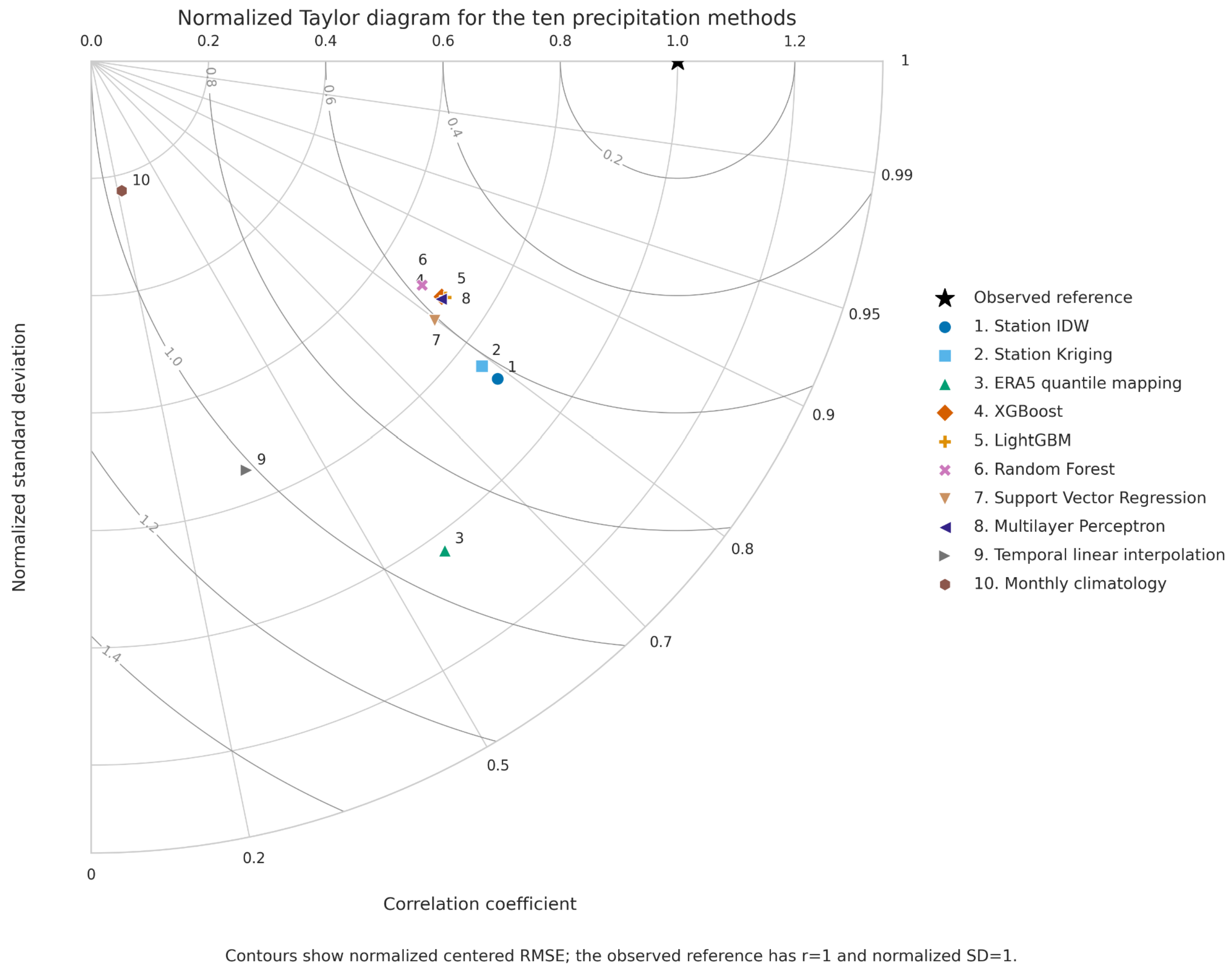
The joint behaviour of correlation, variability, and centred error is summarized in the normalized Taylor diagram presented in Figure 4.

The full-hybrid machine-learning models were positioned closest to the observed reference because of their higher correlations and lower centred errors. LightGBM, XGBoost, Random Forest, and MLP formed a compact group, whereas IDW and Kriging showed moderately lower correlation and greater centred error. ERA5-EQM and the simple baselines were located farther from the observed reference, reflecting their weaker reproduction of daily variability.

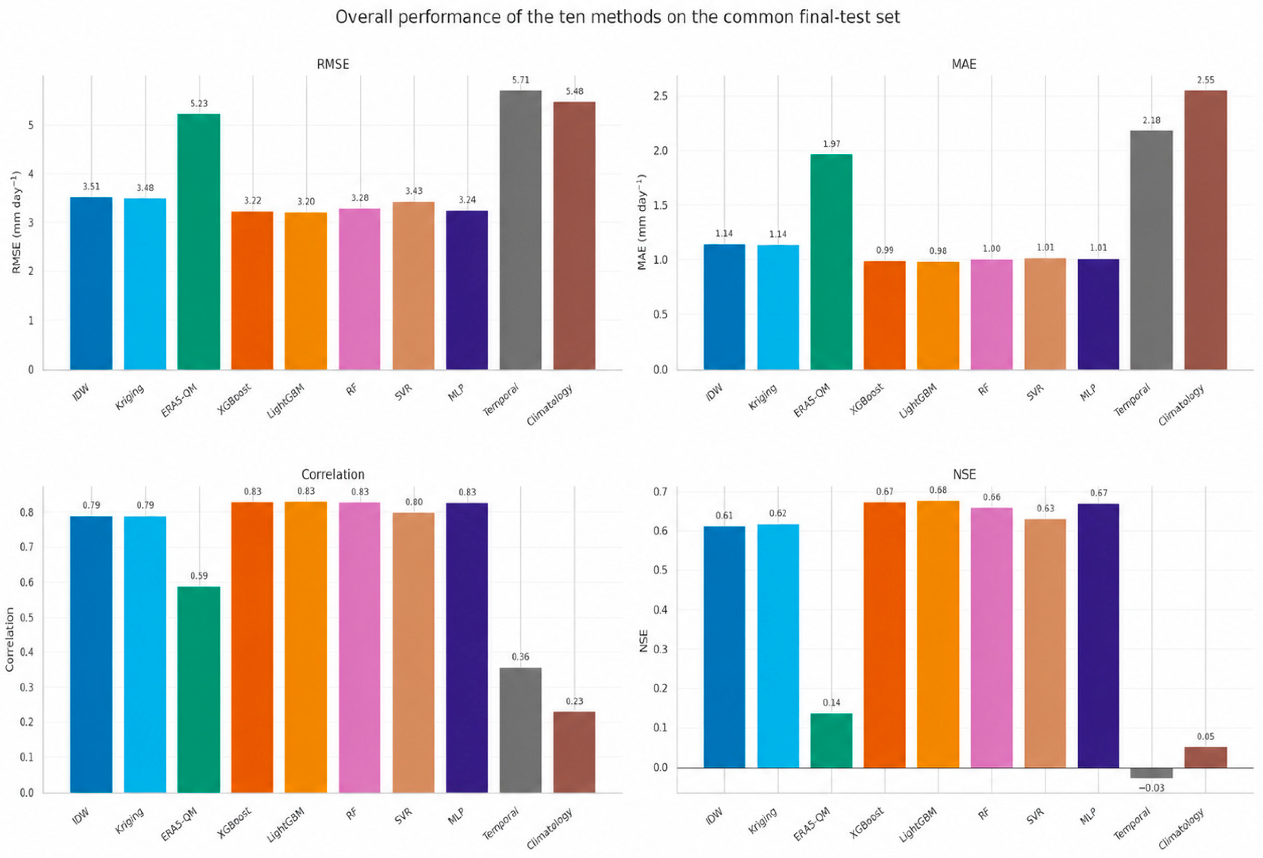
The relative ranking of the methods according to the four principal evaluation measures is shown graphically in Figure 5.

LightGBM achieved the lowest RMSE and MAE and the highest NSE, closely followed by XGBoost, MLP, and Random Forest. Kriging and IDW remained strong deterministic benchmarks, whereas ERA5-EQM and the two simple baselines produced substantially lower overall performance.

Station-level variation in model performance was evaluated using the RMSE, MAE, Pearson correlation, and NSE values presented in Supplementary Figure S2.

As shown in Supplementary Figure S2, the station-wise results indicate that the superiority of the full-hybrid models was not restricted to a single station. LightGBM, XGBoost, Random Forest, and MLP generally produced lower errors and higher NSE values across most of the network. Performance nevertheless varied among stations, with larger errors occurring at some more difficult locations. The simple baselines showed consistently lower correlation and NSE values and greater spatial variability in error.

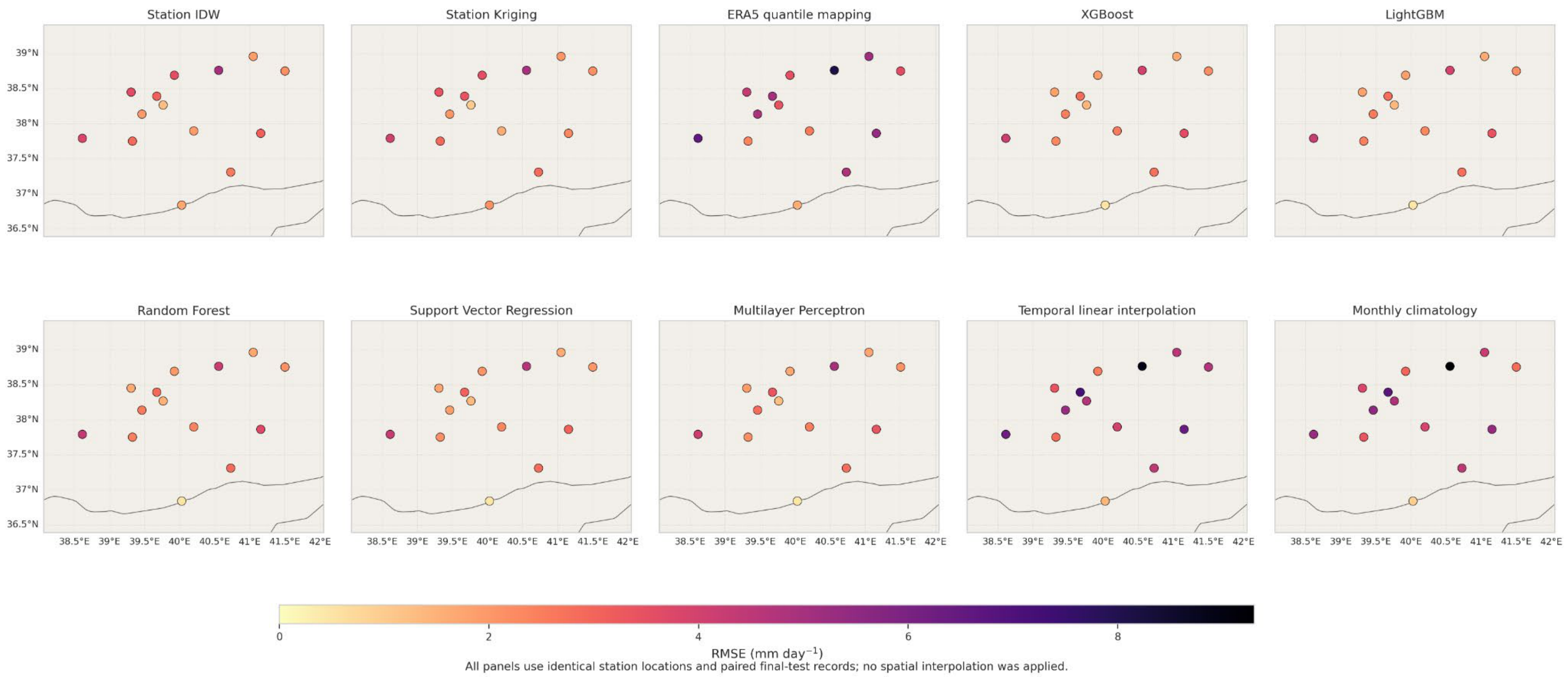
To examine spatial behaviour during a common representative period, calendar year 2005 was selected using observed precipitation and sampling coverage only. The selected year represented all 14 stations with sufficient final-test records and was not chosen according to the performance of any method. Figure 6 presents the station-wise RMSE values for this year without applying an additional interpolation between stations.

The 2005 maps show that reconstruction difficulty varied spatially across the station network. The full-hybrid models generally produced lower and more spatially uniform RMSE values than ERA5-EQM and the simple baselines. IDW and Kriging provided competitive spatial performance, although localized differences remained among stations. Temporal linear interpolation and monthly climatology showed both higher errors and stronger station-to-station contrasts.

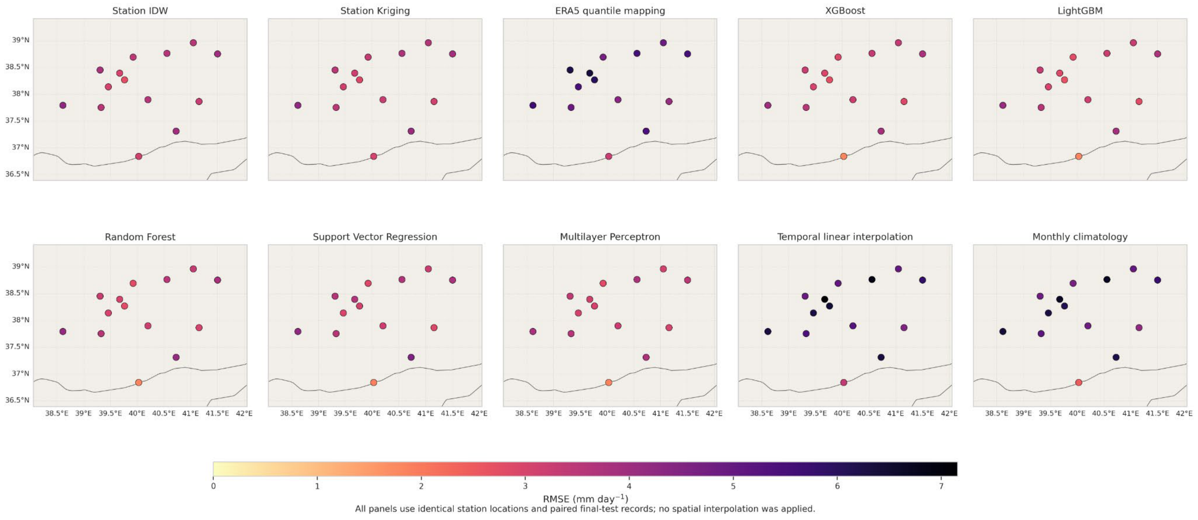
The persistence of these spatial patterns over the complete study period was examined using the long-term station-wise RMSE distributions shown in Figure 7.

The long-term maps confirm that the spatial performance patterns observed in 2005 were broadly representative of the complete evaluation period. The hybrid machine-learning models maintained comparatively low RMSE values across most stations, whereas ERA5-EQM and the simple baselines showed consistently higher errors. The improvement obtained from combining local gauge information, Kriging, and ERA5-Land covariates was therefore distributed across the network rather than being driven by a single station or a single year.

3.7. Statistical Significance of Model Differences

To assess whether differences between the best-performing model and the remaining simple, spatial, reanalysis, and machine-learning methods were statistically meaningful, pairwise Wilcoxon signed-rank tests were applied to the absolute residual-error series. Full-hybrid LightGBM, which achieved the lowest RMSE on the independent final-test dataset, was used as the reference model. The results are presented in

Table 7. Pairwise Wilcoxon signed-rank tests relative to LightGBM.

Model	Wilcoxon W	p-Value
IDW	9.1786 × 107	<0.001
Kriging	8.92465 × 107	<0.001
ERA5_EQM	9.13414 × 107	<0.001
XGBoost	1.26152 × 108	2.4822 × 10−6
RF	1.22550 × 108	9.1666 × 10−17
SVR	8.36836 × 107	<0.001
MLP	1.09759 × 108	5.2633 × 10−99
Station-month climatological mean	2.42403 × 107	<0.001
Temporal linear interpolation	1.18731 × 108	6.6442 × 10−34

.

All pairwise comparisons were statistically significant at the 95% confidence level. The difference between LightGBM and its closest competitor, XGBoost, was significant (p = 2.4822 × 10⁻⁶), although their absolute RMSE difference was small. Therefore, statistical significance was interpreted together with effect size: XGBoost and MLP remained practically close alternatives, whereas the differences against temporal linear interpolation, the station-month climatological mean, IDW, Kriging, and ERA5-EQM were both statistically and practically substantial. These results strengthen the evidence that the proposed ERA5-supported spatial hybrid framework outperformed lower-complexity reference approaches on the common final-test records.

3.8. Spatial Autocorrelation of Residuals

The spatial stability and potential spatial bias of the best-performing LightGBM model were evaluated using Global Moran’s I analysis applied to station-based residual errors [37]. The calculated Global Moran’s I value was −0.0337. Because this value is very close to zero, the residuals do not show a pronounced spatial clustering pattern. The weak negative value suggests that model errors are distributed largely randomly across the station network rather than being systematically concentrated in a specific geographical or topographic zone. This result supports the spatial stability of the developed model across the study area.

4. Discussion

Performance improved progressively as station-internal temporal information was supplemented with same-day spatial predictors and ERA5-Land atmospheric covariates. The simple baselines used only the target-station series, deterministic methods represented spatial dependence, and the hybrid models combined spatial, temporal, station, and reanalysis information within a two-stage occurrence-amount framework. This progression explains the superior performance of the full-hybrid LightGBM model.

Full-hybrid models achieved NSE values above 0.62, while optimized Kriging and IDW also exceeded 0.60. In contrast, the simple baselines and direct ERA5-EQM replacement produced substantially lower NSE values, confirming the value of explicit spatial and atmospheric information.

4.1. Simple Temporal-Statistical and Deterministic Spatial Baselines

Although the archive-wide missing-data ratio was only 0.57%, the two station-internal baselines performed substantially worse under the common controlled test. This reflects the intermittent and event-driven nature of daily precipitation, for which monthly averages and local temporal continuity provide limited information about individual rainfall events [7,8]. The simple methods nevertheless remain useful transparent benchmarks.

Kriging and IDW outperformed the basic machine-learning models when explicit Kriging and ERA5-Land predictors were absent. Lupi et al. [13] likewise found that greater model complexity did not necessarily improve rainfall reconstruction when predictor information was limited, whereas Chivers et al. [12] reported gains from a two-stage framework that combined environmental variables and neighbouring gauges. These comparisons indicate that machine-learning performance depends strongly on whether the predictor set represents concurrent spatial dependence and atmospheric variability.

4.2. Importance of Spatial Autocorrelation and Kriging-Derived Features

The SHAP ranking and the Kriging-supported results both indicate the importance of spatial information. The Kriging feature had the largest attribution, and adding it improved every machine-learning model relative to the basic scenario. This agrees with precipitation-recovery studies in which neighbouring-gauge information was among the most useful inputs [12,13]. MLP was the best Kriging-supported regressor, whereas LightGBM became the best model after ERA5-Land covariates were added, showing that the preferred learner can vary with predictor composition.

The pooled semivariogram describes the average same-day spatial pattern, while local Kriging was fitted separately for each target station-day. All-zero or effectively constant neighbourhoods produced zero or constant-mean estimates; mixed wet and dry neighbourhoods could smooth localized rainfall. This supports the use of standalone Kriging as a spatial benchmark and predictor rather than as a complete occurrence-amount model.

4.3. ERA5 as an Auxiliary Covariate Rather than a Direct Replacement

Direct ERA5-EQM replacement was less accurate than the station-based spatial and hybrid methods (RMSE = 5.2252 mm; NSE = 0.1394), indicating that gridded precipitation alone did not adequately reproduce localized daily rainfall. By contrast, ERA5-Land covariates improved the full-hybrid models. This pattern is consistent with precipitation-merging studies in which gridded products were most effective when combined with gauge, coordinate, elevation, and other environmental information [21,38].

4.4. Model Robustness, Statistical Evidence, and Spatial Stability

The experimental design strengthens the reliability of the findings. The closest comparison studies also used random, non-blocked partitions: random five-fold cross-validation in Chivers et al. [12] and Papacharalampous et al. [38], a random three-fold split in Tyralis et al. [21], and a random 60/20/20 training-validation-test split in Lupi et al. [13]. These similarities make directional model-performance comparisons more relevant, although numerical metrics remain dataset-specific. In the present study, the independent test dataset contained 22,878 observations and was excluded from climatological-statistic calculation, interpolation fitting, hyperparameter optimization, variogram selection, SHAP analysis, and cross-validation. Wilcoxon tests showed that absolute residual differences between LightGBM and every comparator, including the two simple baselines, were statistically significant at the 95% confidence level, while Global Moran’s I = −0.0337 indicated no meaningful spatial clustering of residual errors. Together, these findings suggest that LightGBM’s advantage was not solely attributable to random sampling variability or spatially concentrated errors. The site-to-site variation in the best regression algorithm reported by Chivers et al. [12], and the dependence of errors on disagreement between target and neighbouring gauges reported by Lupi et al. [13], further support interpreting model rankings as conditional on input coherence and local network structure.

The graphical diagnostics demonstrate that daily reconstruction accuracy, preservation of variability, and spatial consistency represent complementary dimensions of model performance. IDW and Kriging remained effective spatial benchmarks, whereas the full-hybrid models achieved lower individual-record errors and generally more consistent performance across stations. The increasing dispersion at high precipitation amounts also indicates that extreme daily rainfall remains the most challenging component of the imputation problem.

The results support hybrid models when neighbouring-station and reanalysis data are available, while simple baselines remain useful for transparent benchmarking. The reported performance applies primarily to isolated or irregular station-day gaps with contemporaneous neighbouring observations; transferability to long gaps, network-wide outages, and ungauged stations requires separate blocked validation.

5. Conclusions

This study evaluated simple station-internal baselines, deterministic spatial interpolation, direct ERA5-EQM replacement, and hybrid machine-learning models for daily precipitation imputation. The main conclusions are as follows:

• The leakage-controlled design separated the independent final-test set from calibration, SHAP analysis, variogram selection, hyperparameter optimization, and cross-validation.
• The station-month climatological mean and temporal linear interpolation performed substantially worse than optimized IDW, Kriging, and the hybrid models.
• The full-hybrid LightGBM model achieved the best final-test performance (RMSE = 3.2001 mm; MAE = 0.9814 mm; Pearson r = 0.8317; NSE = 0.6772).
• Optimized IDW and Kriging remained strong benchmarks, and adding the Kriging-derived predictor improved all machine-learning models relative to the basic scenario.
• ERA5-EQM was weak as a direct replacement, whereas ERA5-Land covariates improved performance when combined with station, spatial, temporal, and topographic predictors.

Overall, the most reliable daily precipitation estimates were obtained by combining local observations, same-day spatial information, and ERA5-Land covariates within a rigorously separated training-validation-testing framework.

References

1. Plummer, N.; Allsopp, T.; Lopez, J.A. Guidelines on Climate Change Observation Networks and Systems; World Meteorological Organization: Geneva, Switzerland, 2003. [Google Scholar]
2. McCabe, M.F.; Rodell, M.; Alsdorf, D.E.; Miralles, D.G.; Uijlenhoet, R.; Wagner, W.; Lucieer, A.; Houborg, R.; Verhoest, N.E.C.; Franz, T.E.; et al. The Future of Earth Observation in Hydrology. Hydrol. Earth Syst. Sci. 2017, 21, 3879–3914. [Google Scholar] [CrossRef] [Scilit] [PubMed]
3. Massetti, L. Analysis and Estimation of the Effects of Missing Values on the Calculation of Monthly Temperature Indices. Theor. Appl. Climatol. 2014, 117, 511–519. [Google Scholar]
4. Varotsos, K.V.; Katavoutas, G.; Giannakopoulos, C. On the Use of Reanalysis Data to Reconstruct Missing Observed Daily Temperatures in Europe over a Lengthy Period of Time. Sustainability 2023, 15, 7081. [Google Scholar] [CrossRef] [Scilit]
5. Hersbach, H.; Bell, B.; Berrisford, P.; Hirahara, S.; Horányi, A.; Muñoz-Sabater, J.; Nicolas, J.; Peubey, C.; Radu, R.; Schepers, D.; et al. The ERA5 Global Reanalysis. Q. J. R. Meteorol. Soc. 2020, 146, 1999–2049. [Google Scholar] [CrossRef] [Scilit]
6. Muñoz-Sabater, J.; Dutra, E.; Agustí-Panareda, A.; Albergel, C.; Arduini, G.; Balsamo, G.; Boussetta, S.; Choulga, M.; Harrigan, S.; Hersbach, H.; et al. ERA5-Land: A State-of-the-Art Global Reanalysis Dataset for Land Applications. Earth Syst. Sci. Data 2021, 13, 4349–4383. [Google Scholar] [CrossRef] [Scilit]
7. Burden, R.L.; Faires, J.D. Numerical Analysis, 9th ed.; Brooks/Cole: Boston, MA, USA, 2011. [Google Scholar]
8. Sattari, M.T.; Rezazadeh-Joudi, A.; Kusiak, A. Assessment of Different Methods for Estimation of Missing Data in Precipitation Studies. Hydrol. Res. 2017, 48, 1032–1044. [Google Scholar]
9. Shepard, D. A Two-Dimensional Interpolation Function for Irregularly-Spaced Data. In Proceedings of the 1968 ACM National Conference; ACM Press: New York, NY, USA, 1968; pp. 517–524. [Google Scholar]
10. Krige, D.G. A Statistical Approach to Some Basic Mine Valuation Problems. J. Chem. Metall. Min. Soc. S. Afr. 1951, 52, 119–139. [Google Scholar]
11. Matheron, G. Principles of Geostatistics. Econ. Geol. 1963, 58, 1246–1266. [Google Scholar] [CrossRef] [Scilit]
12. Chivers, B.D.; Wallbank, J.; Cole, S.J.; Sebek, O.; Stanley, S.; Fry, M.; Leontidis, G. Imputation of Missing Sub-Hourly Precipitation Data in a Large Sensor Network: A Machine Learning Approach. J. Hydrol. 2020, 588, 125126. [Google Scholar] [CrossRef] [Scilit]
13. Lupi, A.; Luppichini, M.; Barsanti, M.; Bini, M.; Giannecchini, R. Machine Learning Models to Complete Rainfall Time Series Databases Affected by Missing or Anomalous Data. Earth Sci. Inform. 2023, 16, 3717–3728. [Google Scholar] [CrossRef] [Scilit]
14. Vidal-Paz, J.; Rodríguez-Gómez, B.A.; Orosa, J.A. A Comparison of Different Methods for Rainfall Imputation: A Galician Case Study. Appl. Sci. 2023, 13, 12260. [Google Scholar] [CrossRef] [Scilit]
15. Chen, T.; Guestrin, C. XGBoost: A Scalable Tree Boosting System. In Proceedings of the 22nd ACM SIGKDD International Conference on Knowledge Discovery and Data Mining, San Francisco, CA, USA, 13–17 August 2016; Association for Computing Machinery: New York, NY, USA, 2016; pp. 785–794. [Google Scholar] [CrossRef] [Scilit]
16. Ke, G.; Meng, Q.; Finley, T.; Wang, T.; Chen, W.; Ma, W.; Ye, Q.; Liu, T.-Y. LightGBM: A Highly Efficient Gradient Boosting Decision Tree. In Proceedings of the 31st International Conference on Neural Information Processing Systems; Curran Associates Inc.: Red Hook, NY, USA, 2017; Volume 30, pp. 3146–3154. [Google Scholar]
17. Breiman, L. Random Forests. Mach. Learn. 2001, 45, 5–32. [Google Scholar] [CrossRef] [Scilit]
18. Hornik, K.; Stinchcombe, M.; White, H. Multilayer Feedforward Networks Are Universal Approximators. Neural Netw. 1989, 2, 359–366. [Google Scholar] [CrossRef] [Scilit]
19. Cortes, C.; Vapnik, V. Support-Vector Networks. Mach. Learn. 1995, 20, 273–297. [Google Scholar] [CrossRef] [Scilit]
20. Smola, A.J.; Schölkopf, B. A Tutorial on Support Vector Regression. Stat. Comput. 2004, 14, 199–222. [Google Scholar] [CrossRef] [Scilit]
21. Tyralis, H.; Papacharalampous, G.A.; Doulamis, N.; Doulamis, A. Merging Satellite and Gauge-Measured Precipitation Using LightGBM with an Emphasis on Extreme Quantiles. IEEE J. Sel. Top. Appl. Earth Obs. Remote Sens. 2023, 16, 6969–6979. [Google Scholar] [CrossRef] [Scilit]
22. Lundberg, S.M.; Lee, S.-I. A Unified Approach to Interpreting Model Predictions. In Advances in Neural Information Processing Systems 30; Curran Associates, Inc.: Red Hook, NY, USA, 2017; pp. 4765–4774. [Google Scholar]
23. Republic of Türkiye Ministry of Agriculture and Forestry, General Directorate of Water Management. Fırat-Dicle Havzası, Dicle Alt Havzası Taşkın Yönetim Planı: Yönetici Özeti [Euphrates–Tigris Basin, Tigris Sub-Basin Flood Management Plan: Executive Summary]. Available online: https://www.tarimorman.gov.tr/SYGM/Sayfalar/Detay.aspx?SayfaId=53 (accessed on 21 May 2026).
24. Turkish State Meteorological Service. Official Climate Statistics—Diyarbakır. Available online: https://www.mgm.gov.tr/veridegerlendirme/il-ve-ilceler-istatistik.aspx?k=&m=DIYARBAKIR (accessed on 21 May 2026).
25. Sun, Q.; Miao, C.; Duan, Q.; Ashouri, H.; Sorooshian, S.; Hsu, K.-L. A Review of Global Precipitation Data Sets: Data Sources, Estimation, and Intercomparisons. Rev. Geophys. 2018, 56, 79–107. [Google Scholar] [CrossRef] [Scilit]
26. El Hachem, A.; Seidel, J.; Imbery, F.; Junghänel, T.; Bárdossy, A. Technical Note: Space-Time Statistical Quality Control of Extreme Precipitation Observations. Hydrol. Earth Syst. Sci. 2022, 26, 6137–6146. [Google Scholar] [CrossRef] [Scilit]
27. Alduchov, O.A.; Eskridge, R.E. Improved Magnus Form Approximation of Saturation Vapor Pressure. J. Appl. Meteorol. Climatol. 1996, 35, 601–609. [Google Scholar] [CrossRef] [Scilit]
28. Lawrence, M.G. The Relationship between Relative Humidity and the Dewpoint Temperature in Moist Air: A Simple Conversion and Applications. Bull. Am. Meteorol. Soc. 2005, 86, 225–233. [Google Scholar] [CrossRef] [Scilit]
29. Hengl, T.; Nussbaum, M.; Wright, M.N.; Heuvelink, G.B.M.; Gräler, B. Random Forest as a Generic Framework for Predictive Modelling of Spatial and Spatio-Temporal Variables. PeerJ 2018, 6, e5518. [Google Scholar] [CrossRef] [Scilit] [PubMed]
30. Friedman, J.H. Greedy Function Approximation: A Gradient Boosting Machine. Ann. Stat. 2001, 29, 1189–1232. [Google Scholar] [CrossRef] [Scilit]
31. Qiu, H.; Chen, H.; Xu, B.; Liu, G.; Huang, S.; Nie, H.; Xie, H. Multiple Types of Missing Precipitation Data Filling Based on Ensemble Artificial Intelligence Models. Water 2024, 16, 3192. [Google Scholar] [CrossRef] [Scilit]
32. Boukdire, M.; İnan, Ç.A.; Varra, G.; Della Morte, R.; Cozzolino, L. Interpolation and Machine Learning Methods for Sub-Hourly Missing Rainfall Data Imputation in a Data-Scarce Environment: One- and Two-Step Approaches. Hydrology 2025, 12, 297. [Google Scholar] [CrossRef] [Scilit]
33. Rumelhart, D.E.; Hinton, G.E.; Williams, R.J. Learning Representations by Back-Propagating Errors. Nature 1986, 323, 533–536. [Google Scholar] [CrossRef] [Scilit]
34. Déqué, M. Frequency of Precipitation and Temperature Extremes over France in an Anthropogenic Scenario: Model Results and Statistical Correction According to Observed Values. Glob. Planet. Change 2007, 57, 16–26. [Google Scholar] [CrossRef] [Scilit]
35. Gudmundsson, L.; Bremnes, J.B.; Haugen, J.E.; Engen-Skaugen, T. Technical Note: Downscaling RCM Precipitation to the Station Scale Using Statistical Transformations—A Comparison of Methods. Hydrol. Earth Syst. Sci. 2012, 16, 3383–3390. [Google Scholar] [CrossRef] [Scilit]
36. Themeßl, M.J.; Gobiet, A.; Leuprecht, A. Empirical-Statistical Downscaling and Error Correction of Daily Precipitation from Regional Climate Models. Int. J. Climatol. 2011, 31, 1530–1544. [Google Scholar] [CrossRef] [Scilit]
37. Moran, P.A. Notes on Continuous Stochastic Phenomena. Biometrika 1950, 37, 17–23. [Google Scholar] [CrossRef] [Scilit] [PubMed]
38. Papacharalampous, G.A.; Tyralis, H.; Doulamis, A.; Doulamis, N. Comparison of Machine Learning Algorithms for Merging Gridded Satellite and Earth-Observed Precipitation Data. Water 2023, 15, 634. [Google Scholar] [CrossRef] [Scilit]
Figure 1. Location of the study area. (a) Regional location of the study area within Türkiye and the surrounding countries; (b) enlarged map of the study area centred on Diyarbakır Province, showing the Euphrates and Tigris sub-basins and the meteorological observation stations.
Atmosphere 17 00727 g001
Figure 2. Leakage-controlled experimental design and comparison of daily precipitation-imputation scenarios. (a) Independent final-test separation, five-fold model development, predictor construction, and final evaluation; (b) predefined predictor groups and the compared imputation scenarios, including simple station-internal baselines, direct ERA5-Land correction, deterministic interpolation, and the basic, Kriging-supported, and full-hybrid machine-learning models.
Atmosphere 17 00727 g002
Figure 3. Pooled same-day empirical semivariogram of daily precipitation.
Atmosphere 17 00727 g003
Figure 4. Normalized Taylor diagram summarizing Pearson correlation, normalized standard deviation, and normalized centred RMSE for the ten methods relative to the observed precipitation from the final test. The star indicates the observed reference.
Atmosphere 17 00727 g004
Figure 5. Overall RMSE, MAE, Pearson correlation, and NSE of the ten precipitation-imputation methods on the common independent final-test set. Each color represents a different precipitation-imputation method and is used consistently across all four panels.
Atmosphere 17 00727 g005
Figure 6. Station-wise RMSE of the ten methods during the objectively selected calendar year 2005. Each symbol represents the RMSE calculated from the matched final-test records at one station. A common colour scale is used across all panels, and no spatial interpolation was applied between stations.
Atmosphere 17 00727 g006
Figure 7. Long-term station-wise RMSE of the ten precipitation-imputation methods on the independent final-test records during 1985–2014. A common colour scale is used across all panels, and no spatial interpolation was applied between stations.
Atmosphere 17 00727 g007