Article

Impact of Optical Flow and Joint Loss on Nowcasting of Severe Convective Weather at Airports
1
Guanghan Branch, Civil Aviation Flight University of China, Guanghan 618307, China
2
Meteorological Center of Southwest Air Traffic Control Bureau, Chengdu 610200, China
*
Author to whom correspondence should be addressed.
Atmosphere 2026, 17(5), 497; https://doi.org/10.3390/atmos17050497
Submission received: 17 March 2026 / Revised: 29 April 2026 / Accepted: 6 May 2026 / Published: 14 May 2026

Abstract

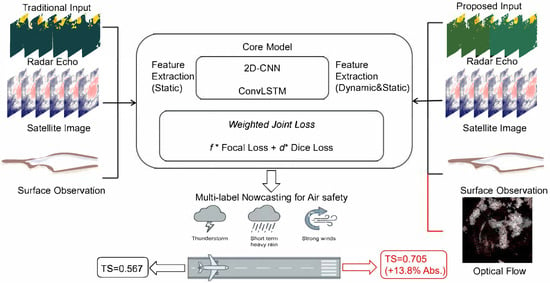
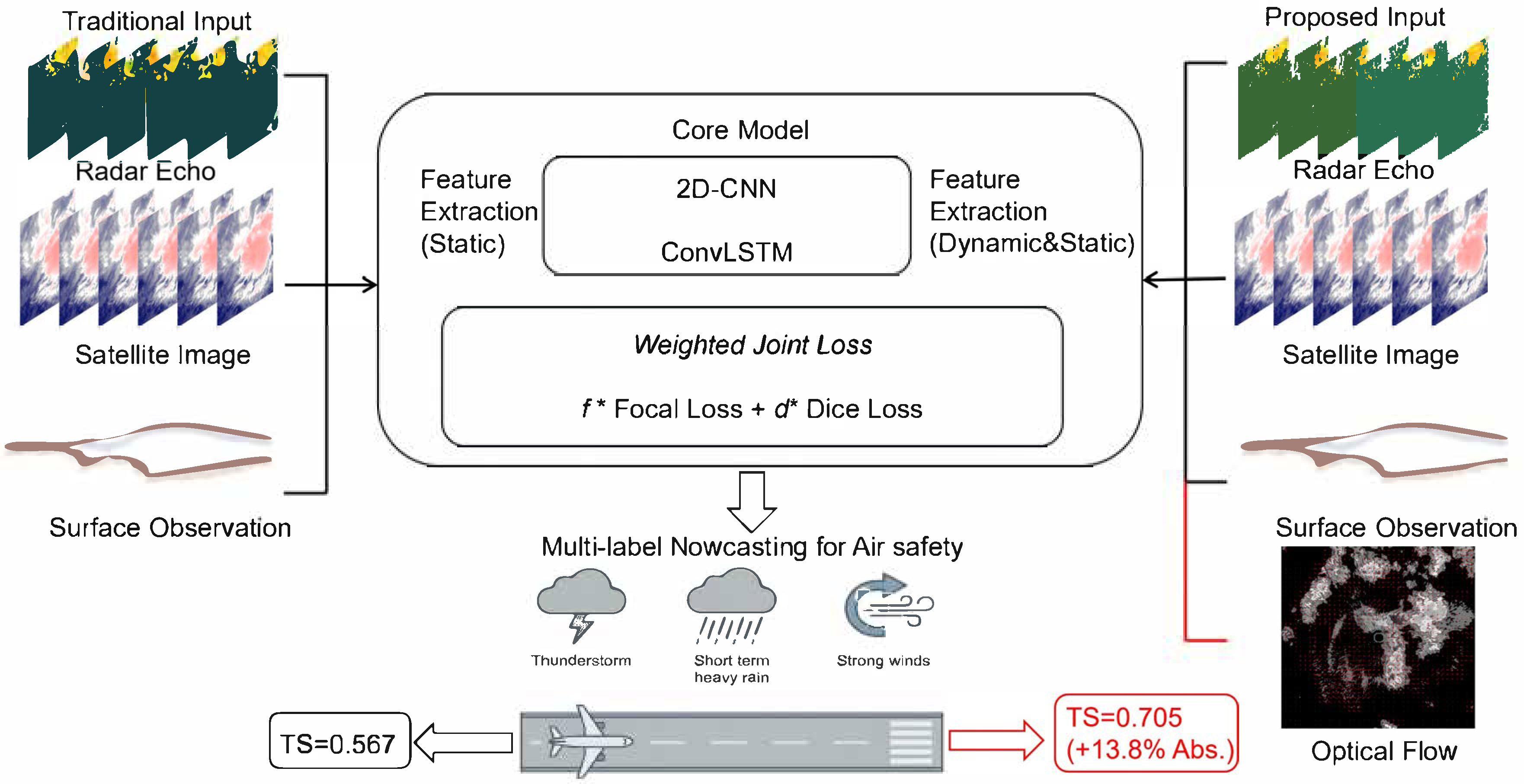
With the increasing frequency of extreme weather and rapid growth of civil aviation, severe convective weather (thunderstorms, short-term heavy precipitation, and strong winds) poses growing threats to flight safety. This study proposes a multi-label CNN-ConvLSTM framework that fuses airport Doppler radar echoes, Himawari-8 satellite imagery, surface observations, and radar optical flow features to nowcast multiple severe convective events within the next 30 min. The model uses 2D-CNN for spatial extraction, ConvLSTM for temporal dynamics, and a weighted joint loss (Focal Loss and Dice Loss) to address class imbalance. Trained on 396 samples (positive-to-negative ratio 1:2.5) from 83 events at Guanghan Airport (2021–2024), incorporating optical flow features significantly boosted performance: macro-F1 increased from 0.719 to 0.792, and Threat Score (TS) from 0.567 to 0.705. Notably, false negatives for minority classes dropped sharply, with strong winds F1-score rising from 0.15 to 1.00. Ablation analysis showed optical flow as the top contributor (Mean Decrease in TS ≈ 0.5). Through multi-modal fusion and motion enhancement, this interpretable model provides high-precision nowcasting for airport severe convective weather, offering substantial value for aviation safety.

Graphical Abstract

1. Introduction

High-impact severe convective weather events, known for their sudden onset, short duration, and destructiveness, remain a vital research subject in atmospheric science due to the substantial annual losses in life and property they cause in China [1,2]. Aviation is particularly vulnerable to these events. Severe convection not only poses a threat to the structural safety of aircraft and the stability of flight attitude but also frequently leads to flight delays, returns, and other operational issues, making it one of the main meteorological factors affecting flight safety and normal flight operations [3,4]. Given the increasing frequency of such extreme events under global climate change, there is a pressing need to improve precise forecasting capabilities for different convective weather types in airport terminal areas to safeguard aviation.
For the nowcasting of severe convective weather, early studies primarily relied on subjective analysis based on synoptic principles, threshold-based judgments of single-station radar products, and Numerical Weather Prediction (NWP) products [5,6,7,8,9,10]. These methods laid the groundwork for operational services, but they remain limited in capturing the nonlinear dynamics of severe convective storms, meeting aviation’s minute-level timeliness requirements, and delivering high spatiotemporal-resolution data. In recent years, deep learning techniques have been widely applied to convective nowcasting [11,12]. Through Convolutional Neural Networks (CNN), Long Short-Term Memory networks (LSTM), Convolutional LSTM (ConvLSTM), and TrajGRU, models can not only learn from detection data but also learn from spatiotemporal sequences such as satellite cloud imagery and radar echo maps [13,14,15,16,17,18]. These studies have advanced radar-echo extrapolation and severe convective weather forecasting; however, operational deployment remains hampered by data scarcity and class imbalance, which constrain model performance and generalizability.
Furthermore, the direct application of the aforementioned methods to airport operational support faces two main challenges. Firstly, most of the previous studies are based on a single-label multi-class classification framework [19,20], which can only output mutually exclusive single categories for a given weather event. However, in meteorological support for aviation safety, it is necessary to issue separate warnings for each weather phenomenon, allowing for the simultaneous occurrence of thunderstorms, strong winds, and short-term heavy precipitation, and so on. Secondly, there is a prevailing view that deep learning models lack a fundamental understanding of physical laws, and the rationale behind their decisions lacks systematic explanation [21].
To address these challenges, on one hand, adopting a multi-label binary classification framework can effectively handle the requirement for concurrent warnings of multiple weather phenomena [22]. On the other hand, introducing traditional optical flow technology can enhance the ability of deep learning models to process multi-source heterogeneous data and improve the interpretability of predictions for severe convective weather. As a method based on motion estimation from image sequences, optical flow technology has been widely used in meteorological operations. It can effectively capture the movement characteristics of severe convective systems/cloud clusters by calculating the motion vector fields of radar echoes or satellite cloud imagery [23,24,25,26]. Particularly for weather processes dominated by linear motion, optical flow methods often provide more accurate predictions than purely data-driven approaches [27].
However, current applications of optical flow are mostly limited to using radar-based optical flow alone or integrating various optical flow algorithms [28,29]. These approaches still have limitations in handling nonlinear motion and the genesis/decay of weather systems, and cannot fully enhance the model’s generalization performance and interpretability [26].
To address the aforementioned limitations of existing optical flow approaches while preserving their strength in capturing storm dynamics, this study develops a deep learning model formulated as a multi-label binary classifier that simultaneously and independently produces probability estimates for thunderstorms, strong winds, and short-duration heavy precipitation, thus better addressing operational requirements for issuing concurrent warnings of multiple weather hazards in the terminal area. To further enhance the model’s physical interpretability and forecasting skill, the model integrates multi-source high-resolution observation data (including satellite, radar, and surface observations) and explicitly incorporates motion field features derived from optical flow algorithms to better characterize the movement and developmental evolution of weather systems. By means of several experiments, the contributions of different data sources and of optical-flow features to nowcasting performance will be quantitatively assessed, with the aim of providing a scientific basis and a reference for developing more reliable and interpretable nowcasting methods for severe convective weather at airports.

2. Data and Methods

2.1. Study Area

Guanghan Airport (30.95° N, 104.34° E) is situated on the northern edge of the Chengdu Plain within the Sichuan Basin, China (Figure 1). The Sichuan Basin is a bowl-shaped terrain surrounded by the Tibetan Plateau to the west and the Yunnan-Guizhou Plateau to the south, which facilitates moisture accumulation and convective initiation over the region. The airport operates under a subtropical monsoon climate, where severe convective weather frequently occurs during the warm season (April–September). Guanghan Airport is equipped with comprehensive observational systems including an ADWR-X Doppler weather radar, manufactured by Beijing Leiyin Electronic Technology Co., Ltd. (Leiyin) in Beijing, China, and an automated surface weather station (AWOS), providing high-quality, continuous records suitable for multi-source data fusion and nowcasting research.

2.2. Data Sources and Processing

A multi-modal dataset of 396 samples was constructed from 83 severe convective events that occurred at Guanghan Airport between 2021 and 2024. The dataset includes Doppler weather radar observations covering the airport terminal area, satellite cloud imagery, surface meteorological measurements, and radar-derived optical-flow features. All data were temporally aligned at 10 min intervals and subjected to rigorous quality-control procedures, yielding a positive: negative sample ratio of approximately 1:2.5, positive samples correspond to time periods when the target severe convective weather phenomenon was observed, while negative samples correspond to periods without such event.
Doppler weather radar is a key instrument for airport convective-weather monitoring [30], and its high spatiotemporal-resolution products are essential for detection and forecasting. Radar reflectivity imagery for this study were acquired from the ADWR-X-band terminal Doppler weather radar at Guanghan Airport. The images were center-cropped on the airport, normalized, temporally aligned to 10 min intervals using linear interpolation, and denoised to remove interference.
Satellite cloud imagery was obtained from the Himawari-8 geostationary satellite (located at 140.7° E), which provides 16 spectral bands at 10 min intervals [13]. In this study, three infrared channels were selected: 2.3 μm (near-IR) for cloud microphysical estimation, 6.2 μm (water-vapor absorption) for mid-tropospheric moisture monitoring, and 10.4 μm for cloud-top characterization (ice/water detection).
Surface observations were collected at the midpoint of Guanghan Airport’s runway and comprise per-minute measurements at 10 m of air temperature, wind direction, wind speed, pressure, and relative humidity. Based on pre-convective evolution, 3 h and 24 h changes in temperature and pressure were derived; together with the five basic variables, these form a 9-dimensional feature vector.
All datasets were pre-processed through temporal synchronization (every 10 min), feature extraction, and quality control. This 10 min update cycle is notably finer than many operational nowcasting systems that issue forecasts at 1 h or 3 h intervals. A 30 min forecast lead time is selected because it aligns with the operational safety margin required in airport air traffic management—within this window, controllers have sufficient time to issue advisories and pilots can take protective measures before hazardous weather impacts the terminal area. Further details on the three heterogeneous data sources are provided in Table 1.
To address the class imbalance issue (thunderstorms account for 45% of the validation set, short-term heavy rainfall 24%, and strong winds 21%), the dataset was split into training and test sets in an 8:2 ratio using multi-label stratified sampling. Rare categories (short-term heavy rainfall and strong winds) were augmented through triple oversampling. Data augmentation techniques, including random rotation (±15°), horizontal flipping, and brightness adjustment (±10%), were employed to enhance the model’s generalization capability.

2.3. Definition of Severe Convective Weather

In this study, thunderstorm labels are based on manual observation records from Guanghan Airport, while labels for short-duration heavy rainfall and strong winds come from the airport’s observational data. The detailed labeling criteria are presented in Table 2. The definition of strong winds mainly considers operational thresholds for various aircraft types and refers to the International Civil Aviation Organization (ICAO) wind shear intensity standards [31]. The “more than twice” requirement in Table 2 filters transient gusts that may not produce recognizable remote sensing features. Due to the limited sample size of strong wind events at this location (Guanghan Airport is situated in a region with generally weak wind conditions), this definition employs a composite “OR” criterion, which increases the strong wind sample size while encompassing both sustained strong winds and gust factor deviations. From an operational perspective, both phenomena lead to similar aviation hazards and exhibit similar radar/optical flow signatures.
It is important to highlight that because aircraft takeoffs and landings typically take place within just a few minutes, the definition of short-duration heavy rainfall here places particular emphasis on its impact on flight safety. This differs from most existing studies [32,33], which usually employ cumulative precipitation over 24 h or hourly rainfall data for AI-based modeling. Instead, the present dataset focuses on precipitation intensity at the minute scale, which is more relevant for assessing immediate impacts on flight operations. The thresholds in Table 2 are determined based on a combination of international aviation safety standards, local operational requirements of Guanghan Airport, and domain-specific meteorological conventions.

3. Nowcasting Model for Severe Convective Weather Classification

3.1. Model Overview

In this study, A CNN–ConvLSTM nowcasting framework was developed to predict severe convective weather types up to 30 min in advance by exploiting complementary information from multiple observing platforms. Terminal-area Doppler weather radar images, Himawari-8 satellite cloud images, and surface meteorological observations were temporally synchronized, preprocessed, and fused to provide detailed spatial and thermodynamic context. Radar-derived optical-flow fields were incorporated as an explicit short-term motion prior to quantify storm displacement, supplying reliable minute-scale motion estimates despite the method’s reduced effectiveness at longer lead times due to its linear-motion assumption. Spatial features were extracted via convolutional neural networks (CNN) [34], while ConvLSTM [13] units were used to model the spatiotemporal evolution of the fused representations. By combining a physically interpretable motion prior with nonlinear sequence learning, the architecture leverages multi-source complementarity to enhance short-range forecast accuracy and robustness.
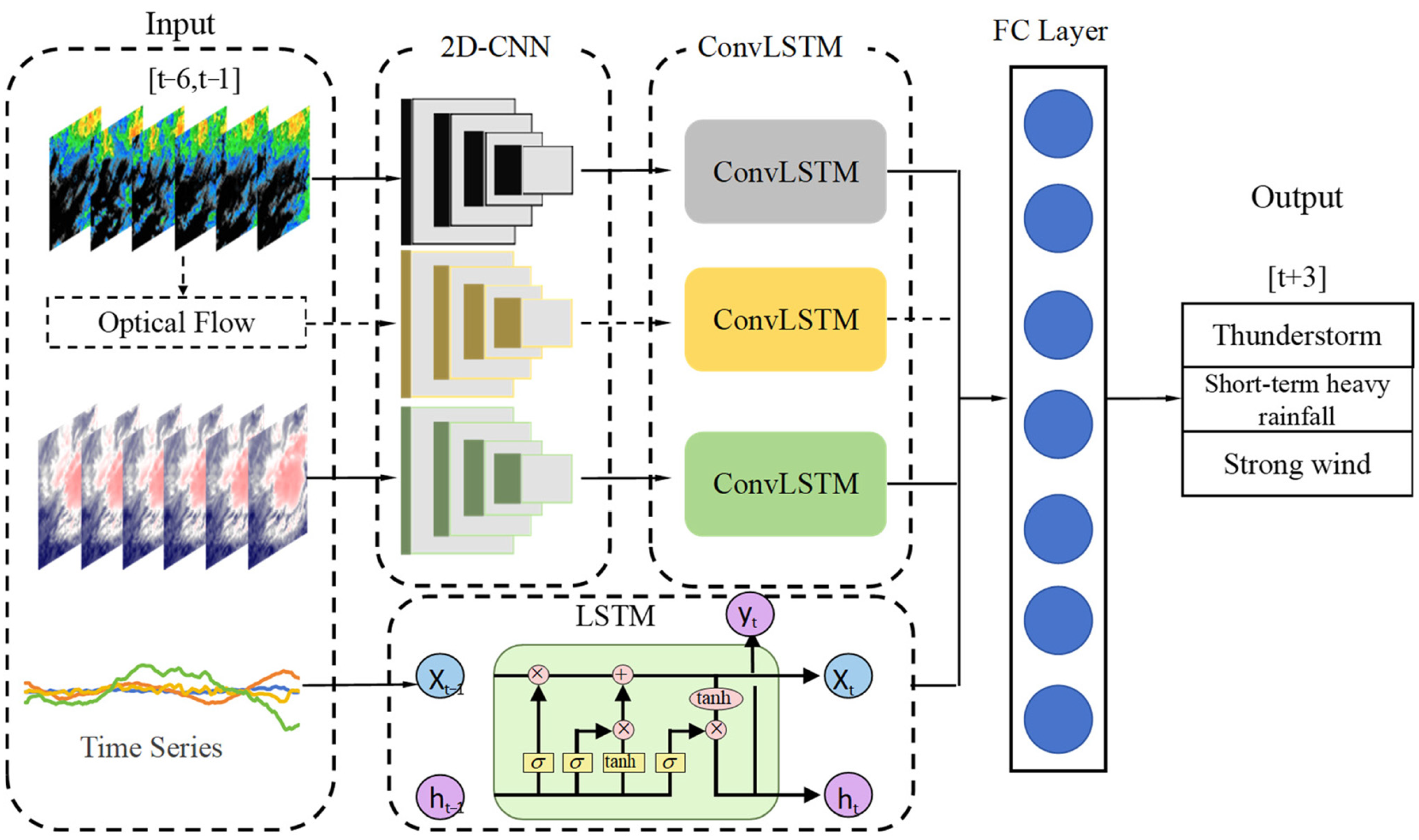
As shown in Figure 2, the model takes multimodal data from the previous hour (six time steps: [t − 6, t − 1]) as input and employs a multi-label binary classification approach to output binary labels for each weather phenomenon (including thunderstorms, short-term heavy rainfall, and strong winds). Spatiotemporal feature extraction is accomplished through 2D-CNN and ConvLSTM.
To analyze the impact of explicitly incorporating radar-derived optical flow features in addition to the input radar temporal characteristics, two CNN-ConvLSTM variants were implemented: a flow-augmented model that incorporates radar-derived optical-flow fields, and a baseline model that omits optical-flow input. Total Variation-L1 (TV-L1) produces smooth motion fields through global optimization and total-variation regularization and has been shown to better capture small-scale motions compared with alternative methods [35,36]. So, optical flow was computed from sequential radar images using the Total Variation-L1 (TV-L1) algorithm.
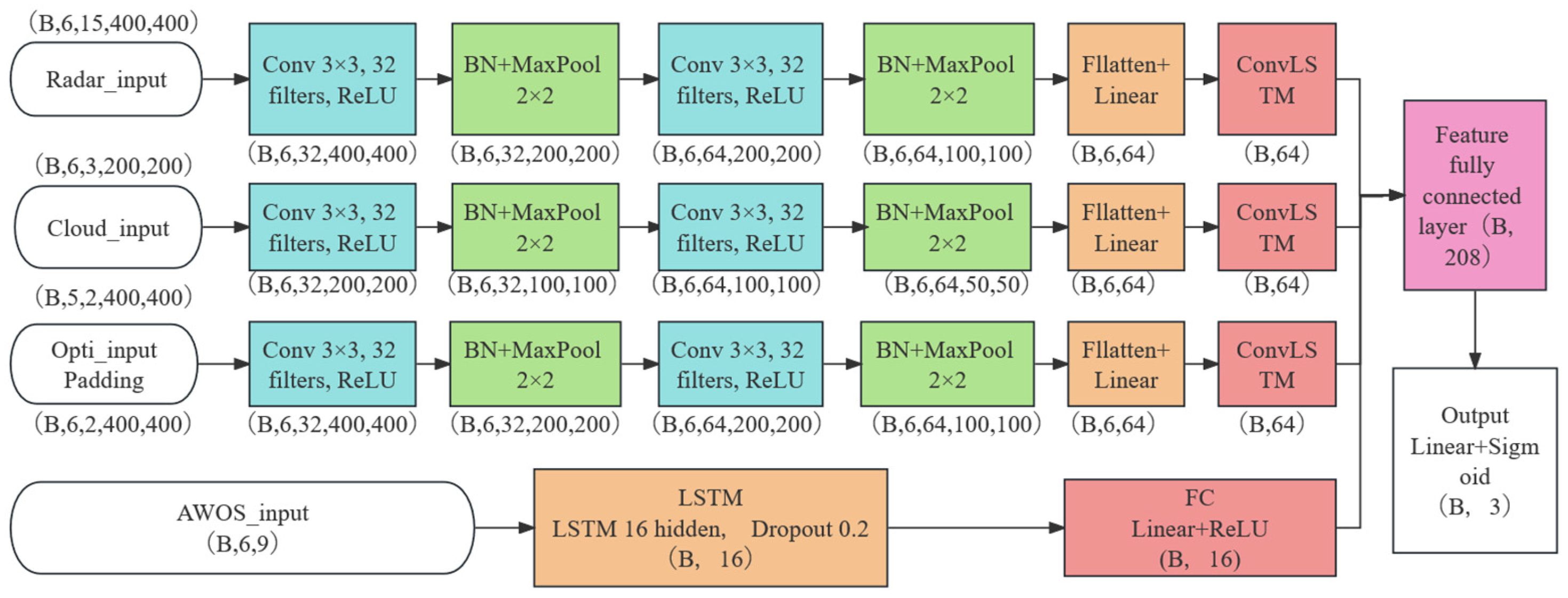
As detailed in Figure 3 (where “B” denotes the batch size), the model architecture consists of three main components. First, a 2D-CNN module processes the spatial features of radar images, satellite cloud images, and the optical flow field (the latter is used only in models incorporating optical flow features). Radar and satellite images are processed through two convolutional layers (with 3 × 3 kernels, filter sizes of 32, and a stride of 1) and BN-MaxPool layers to extract key spatial patterns such as storm cores while reducing dimensionality. The optical flow data passes through two convolutional layers (3 × 3 kernels with 32 filters) and BN-MaxPool layers to extract motion features, enhancing the model’s sensitivity to weather system dynamics.
Second, a temporal modeling module employs LSTM and ConvLSTM to process time-series data from surface meteorological observations and the feature sequences extracted by the 2D-CNN, respectively. The LSTM processes surface meteorological observations through two LSTM layers with dropout (0.2). For the CNN-extracted features, this module contains two ConvLSTM layers (each with 64 filters, and dropout 0.2), effectively preserving spatial and temporal information to capture the nonlinear evolution of storm intensity over time. Compared to traditional RNNs, ConvLSTM mitigates the vanishing gradient problem and is more suitable for spatiotemporal data [37,38].
Finally, in the feature fusion and output module, considering the relatively small dataset size in this study, the model avoids using self-attention-based architectures like Transformers for feature fusion. Instead, the features from ConvLSTM are flattened, and a fully connected layer (64 neurons) integrates the extracted features from both the LSTM and ConvLSTM branches. These are then processed through a Linear + U layer, followed by a final Linear + Sigmoid layer (3 neurons) to generate binary classification probabilities for thunderstorms, short-term heavy rainfall, and strong winds.

3.2. Weighted Joint Loss Function

Sample imbalance in severe convective weather datasets is a well-established challenge. The datasets in this study exhibits not only a positive-negative sample imbalance but also a significant inter-class imbalance. Negative samples dominate the validation set, with positive sample proportions being 45% for thunderstorms, 24% for short-term heavy rainfall, and 21% for strong winds. This distribution may cause the model to favor majority classes and increase the false negative rate.
To address this, a weighted joint loss (CL) function is adopted, combining Focal Loss [39] and Dice Loss [40]. This integrated approach optimizes the model for both hard-to-classify samples and the overlap of predicted labels. The joint loss (CL) is defined as follows:
CL = f × FL(pt) + d × DL
Here, f and d represent the weights assigned to the respective loss functions, used to balance their contributions to the overall loss, with the constraint that their sum equals 1. FL(pt) is based on Binary Cross-Entropy (BCE) loss and incorporates a modulating factor to reduce the influence of easily classified samples. Its formula is defined as:
FL ( p t ) = α ( 1 p t ) γ log ( p t )
Here, FL(pt) represents the Focal Loss value, pt denotes the model’s predicted probability for the correct class, α is the class weighting parameter corresponding to thunderstorms, short-term heavy rainfall, and strong winds, respectively, and γ is the focusing parameter.
DL further optimizes the handling of boundary samples by quantifying the overlap between predictions and ground truth labels. Its formula is given by:
DL   =   1 ( 2   · ( P i · Y i )   +   smooth ) / ( P i     +     Y i +   smooth )
where P and Y, respectively, represent the sum of predicted values and ground truth labels, and smooth is a smoothing term (set to 1.0 to prevent division by zero) [41].

3.3. Model Training and Hyperparameter Tuning

During model training, the dataset was split into training and test sets in an 8:2 ratio using multi-label stratified sampling to ensure a balanced distribution of positive samples for each weather phenomenon in the test set. To enhance validation stability, 5-fold cross-validation was employed. A dropout rate of 0.2 was applied to prevent overfitting, and BatchNorm2d was used to stabilize the training process. All convolutional layers utilized the ReLU activation function to introduce non-linearity [42].
For hyperparameter tuning, an extensive set of experiments was conducted using the grid search method. The optimization primarily focused on the learning rate (Lr) and the parameters of the joint loss (CL) function: the Focal Loss weight f, as well as α and γ. This tuning process aimed to adjust the relative weighting between Focal Loss and Dice Loss, further refine the weighting for minority classes to reduce false negatives, and optimize the overlap for boundary samples.
The experiments were conducted in a Python 3.7.3 environment, with the model implemented and trained using the Keras framework with a TensorFlow backend. Training was performed on a computing platform equipped with an NVIDIA GPU, using a batch size of 16 to balance computational efficiency and model performance.

3.4. Model Evaluation Metrics

Model performance is evaluated using multi-label accuracy, macro-averaged F1-score (F1_macro), ROC-AUC, and the Threat Score (TS) for risk assessment [43].
Multi-label accuracy is a metric used to assess the performance of multi-label classification models. It is calculated by determining whether each label is correctly predicted for each sample and then averaging the results:
Accuracy   = 1 N i = 1 N l ( y i   =   y i )
where N is the number of samples,   y i is the model’s prediction for the i sample,   y i is the ground truth label, and l is the indicator function that equals 1 if the prediction matches the ground truth exactly, and 0 otherwise.
F1-Score represents the harmonic mean of precision and recall, providing a balanced measure of both metrics:
F 1   =   2   ×   P   ×   R P   +   R
where P (Precision) measures the proportion of true positives among all positive predictions, and R (Recall) measures the proportion of actual positives correctly identified. The F1-Score ranges from 0 to 1, with 1 indicating perfect precision and recall, and 0 representing the worst performance. For multi-label classification, we employ macro-averaging (F1_macro) where the metric is computed independently for each class and then averaged.
ROC-AUC measures the classifier’s performance across all possible classification thresholds. A higher Area Under the Curve (AUC) value indicates better classification performance:
AUC   = 0 1 TPR ( FPR ) dFPR
where TPR (True Positive Rate, equivalent to Recall) represents the proportion of actual positives correctly identified, and FPR (False Positive Rate) represents the proportion of actual negatives incorrectly classified as positives. The AUC value ranges from 0 to 1, with values closer to 1 indicating better model performance.
Threat Score (TS) evaluates prediction accuracy by considering true positives, false positives, and false negatives:
TS   =   TP TP   +   FP   +   FN
where TP (true positive or hit) denotes a correctly predicted positive sample; FP (false positive or false alarm) denotes a negative sample incorrectly predicted as positive; and FN (false negative or miss) denotes a positive sample incorrectly predicted as negative. The TS score is particularly valuable for risk assessment in weather forecasting applications.

4. Experimental Results and Model Evaluation

4.1. Sensitivity Analysis of Key Hyperparameters

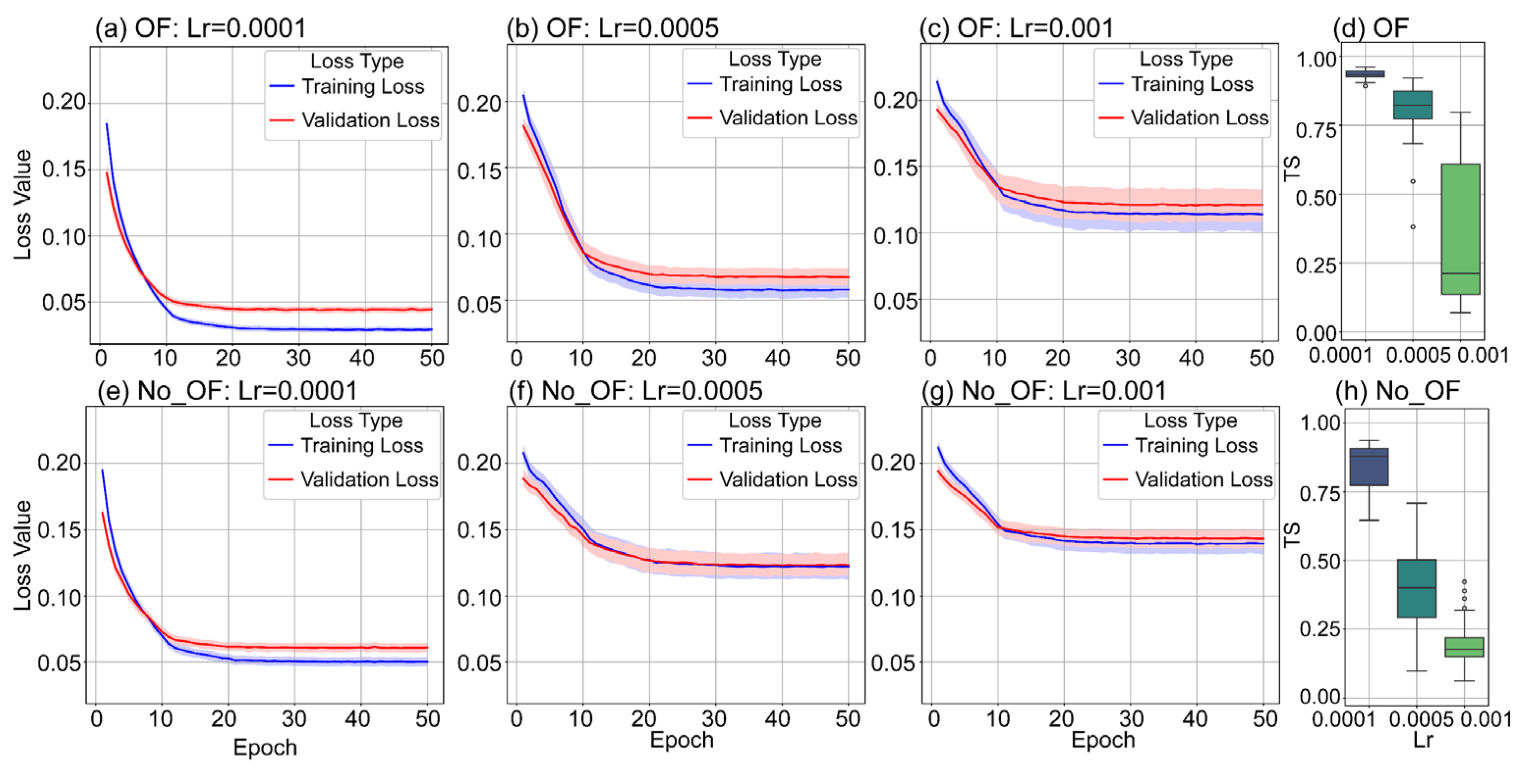
As a key parameter in the optimization process, the learning rate directly influences the model’s convergence speed, loss minimization, and prediction stability. Figure 4 presents the training and validation loss curves as well as the TS (Threat Score) performance of the CNN–ConvLSTM model under different learning rates (lr = 0.0001, 0.0005, and 0.001), for two experimental settings: with and without the inclusion of radar echo optical flow features. The shaded areas represent the 95% confidence intervals, derived from multiple combinations of Focal Loss parameters.
In models incorporating optical flow features (Figure 4a–d), with a learning rate of 0.0001, both training and validation losses decreased rapidly initially before plateauing. The validation loss remained slightly higher than the training loss, indicating stable learning without significant overfitting (Figure 4a). When increased to 0.0005, losses converged faster with lower final values but introduced slight fluctuations (Figure 4b). Further increasing to 0.001 resulted in rapid initial loss decrease followed by a later rise, suggesting potential overfitting (Figure 4c). Regarding TS performance (Figure 4d), the learning rate of 0.0001 achieved the highest and most stable TS (0.705), outperforming 0.0005 (0.682) and 0.001 (0.651), highlighting its advantage in balancing convergence and generalization.
In the models without optical flow features (Figure 4e–h), a similar pattern was observed, lower learning rates (0.0001 and 0.0005) demonstrated greater robustness to parameter variations, as evidenced by narrower confidence intervals and lower validation losses. Conversely, the highest learning rate (0.001) led to increased loss, wider confidence intervals, and indications of overfitting. By comparison, the inclusion of optical flow features resulted in an approximate 0.138 improvement in TS, albeit with increased sensitivity to the choice of learning rate, which suggests that optical flow not only significantly enhances model stability and generalization but also plays an important role in tuning diverse parameter settings. Overall, the results indicate that a learning rate of 0.0005 offers the best balance between convergence speed and robustness under the given experimental conditions.
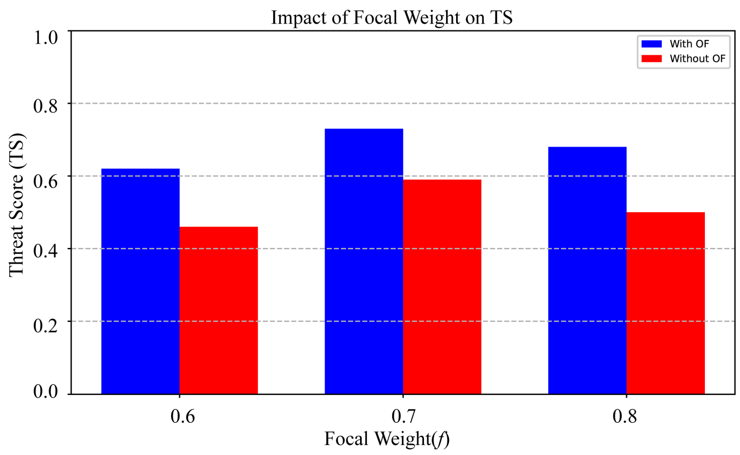
Given the class imbalance in the dataset, the weight parameter (f) of the joint loss function and internal parameters (α and γ) of Focal Loss were critical for performance. Following the learning rate optimization, the influence of these parameters was further investigated. As shown in Figure 5, TS exhibited a non-monotonic trend with varying f in models with radar optical flow features. TS = 0.62 at f = 0.6, peaked at 0.73 when f = 0.7, and decreased to 0.68 when f = 0.8. This indicates that insufficient weighting leads to neglect of difficult samples, whereas excessive weighting results in overfitting. In contrast, models without optical flow consistently showed lower TS values (0.46, 0.59, 0.50), with the peak remaining at 0.59 when f = 0.7, which suggests that optical flow enhanced the model’s sensitivity to parameter optimization, by strengthening the motion information of systems causing severe convective weather, thereby mitigating minority class bias [44].
The aforementioned discrepancy further suggests that the absence of optical flow features may limit the model’s sensitivity to parameter variations. Optical flow models provide more powerful spatiotemporal feature representations by effectively capturing the movement and propagation characteristics of severe convective clouds/echoes [45]. This enhanced representation amplifies the positive impact of f optimization, significantly improving TS scores by effectively addressing class imbalance issues. In contrast, models without optical flow features, relying solely on basic features, cannot overcome performance bottlenecks. Their TS scores stagnated around 0.4, indicating that parameter tuning alone is ineffective without useful features capable of representing the evolution of rare but high-impact weather phenomena.
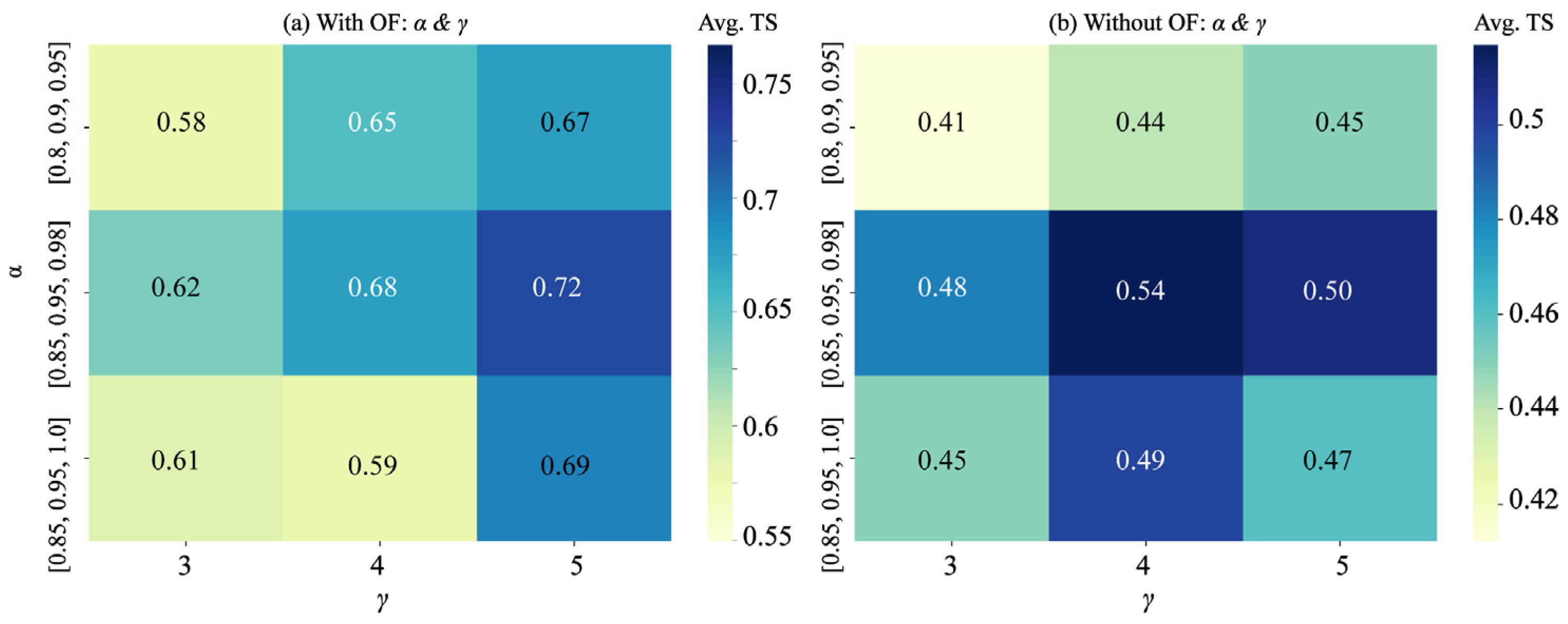
Further analysis of the interaction effects between Focal Loss parameters α (class weights) and γ (focusing parameter) is shown in Figure 6. In models with optical flow (Figure 6a), the highest TS (0.72) was achieved with α = [0.85, 0.95, 0.98] (corresponding to thunderstorms, short-term heavy precipitation, strong winds) and γ = 5, TS decreased to 0.68 when γ = 4 and to 0.62 when γ = 3. This configuration optimized boundary sample handling by increasing minority class weights while suppressing the contribution of easy samples. In models without optical flow (Figure 6b), the peak TS was 0.54 (α = [0.85, 0.95, 0.98], γ = 4), consistently lower than optical flow configurations. The divergent trends confirm the role of optical flow in amplifying positive parameter effects, particularly for minority classes (strong winds).
Based on the comprehensive hyperparameter sensitivity analysis (Figure 4, Figure 5 and Figure 6), optimal configurations were determined through grid search on the validation set. For each parameter combination, the model was trained until convergence (early stopping with patience = 10), and the peak validation TS across all epochs was recorded. The configurations achieving the highest validation performance are summarized in Table 3.

4.2. Performance Evaluation of Optical Flow Fields

Based on the hyperparameter optimization analysis, the overall performance of models with and without radar optical flow features was further evaluated on the test set. As shown in Table 4, incorporating optical flow increased F1_macro from 0.719 to 0.792 (+0.073), TS from 0.567 to 0.705 (+0.138), and ROC-AUC from 0.900 to 0.925, while multi-label accuracy decreased slightly by 0.014. This indicates that optical flow enhanced recall for minority classes (reducing false negatives) but introduced minor misclassifications for majority classes, improving overall generalization capabilities, especially in class-imbalanced scenarios. The significant TS improvement validates the mechanism by which optical flow’s dynamic information (e.g., movement trajectories of severe convective clouds) optimizes ConvLSTM spatiotemporal modeling, consistent with the synergistic effects of learning rate and Focal parameter tuning.
By capturing motion patterns in radar images, optical flow fields enhance the model’s spatiotemporal modeling capabilities, significantly improving prediction accuracy for dynamic weather events (e.g., thunderstorm movement trajectories). Although the limited dataset size imposes constraints on statistical significance testing, the consistent performance gains across experiments provide strong validation of optical flow’s effectiveness. From a mechanistic perspective, the motion vectors derived from optical flow strengthen the ability of the ConvLSTM2d model to track weather system evolution over six time steps. However, how do the models perform for the three severe convective weather categories (thunderstorms, short-term heavy precipitation, and strong winds) with and without optical flow fields? As illustrated by the confusion matrices in Table 5, the incorporation of optical flow exerts a significant positive impact on model prediction performance, with the magnitude of this impact exhibiting distinct variations across different severe convective weather categories.
As shown in Table 5, optical flow incorporation consistently improved prediction performance across all three categories, albeit with varying magnitudes. For heavy rainfall, the F1 score increased from 0.83 to 0.88, with a notable reduction in false negatives indicating enhanced detection capability. The most substantial improvement occurred in strong wind prediction, where the F1 score surged from 0.15 to 1.00, likely attributable to the pronounced flow field characteristics of strong wind events that optical flow effectively captures. For thunderstorms, the F1 score improved from 0.6 to 0.65, representing a more modest gain. This performance may be attributed to the inherent complexity and variability of thunderstorm systems, which poses persistent challenges in distinguishing thunderstorms from other weather categories despite the reduction in false positives.
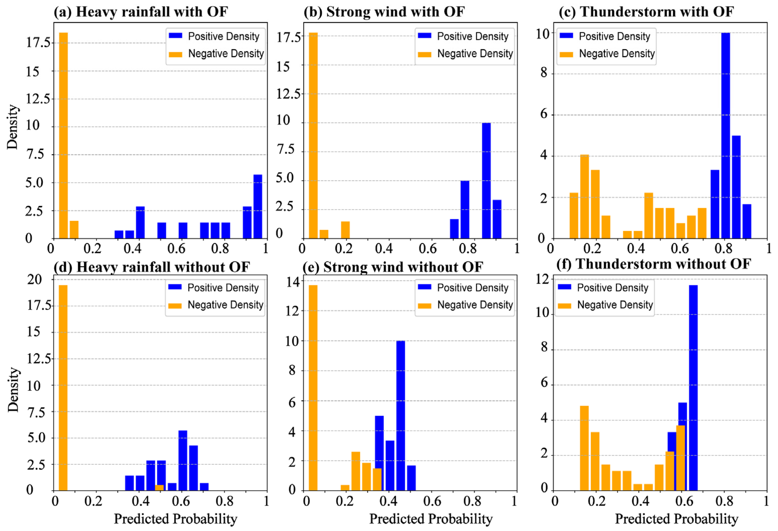
To further validate the role of optical flow features in enhancing classification performance, Figure 7 provides an intuitive perspective through prediction probability distribution histograms for the three severe convective weather phenomena (thunderstorms, short-term heavy precipitation, and strong winds).
In Figure 7a–c, the incorporation of optical flow features substantially improved both probability distribution and classification performance. Positive samples concentrated in the high-probability range (0.8–1.0) while negative samples clustered in the low-probability range (0.0–0.2), whereas the model without optical flow exhibited greater dispersion in positive predictions, particularly in the mid-to-low probability range (0.4–0.7). This distinction aligns with the confusion matrix results in Figure 7, demonstrating that optical flow features effectively mitigated class imbalance by capturing spatiotemporal dynamics of weather systems. For underrepresented categories such as strong winds and heavy rainfall, optical flow significantly reduced false negatives, with F1 scores improving from 0.15 to 1.00 and from 0.83 to 0.88, respectively. Even for thunderstorms, optical flow decreased false positives, improving the F1 score from 0.60 to 0.65. These results indicate that optical flow features not only enhance overall classification performance but also provide effective feature support for minority class optimization.

4.3. Contribution of Multi-Modal Data Fusion

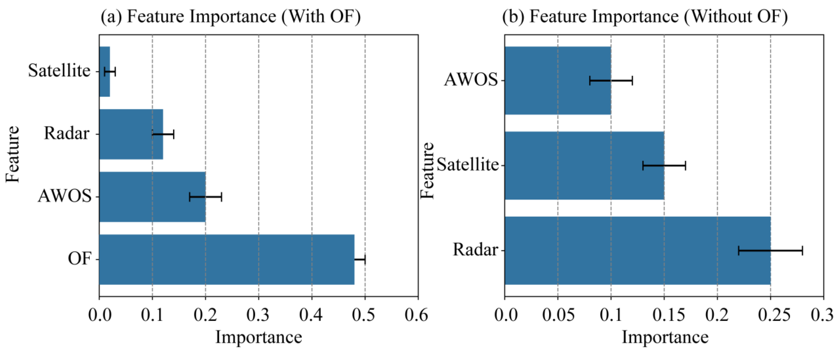
Feature importance analysis of both model groups similarly reveals the critical role of optical flow features in severe convective weather classification and prediction, as shown in Figure 8. Feature contribution is quantified as Mean Decrease in TS (ΔTS), defined as TS (full model) − TS (model without that feature source). Error bars represent the standard deviation across 5-fold cross-validation folds. It is demonstrated that in models incorporating radar optical flow features, optical flow makes the highest contribution (ΔTS ≈ 0.50), significantly exceeding radar (≈0.25), satellite (≈0.15), and AWOS (≈0.10). This underscores the unique value of optical flow in capturing storm dynamics (e.g., convergence movement, convective migration). After removing optical flow, radar became dominant (ΔTS ≈ 0.25), with satellite and AWOS importance decreasing, and AWOS ranking lowest, reflecting compensatory mechanisms and redundancy. The overall importance decreased without optical flow, indicating that single modalities (e.g., radar spatial structures) alone are insufficient to represent dynamic evolution, while the local temporal information from AWOS requires dynamic supplementation.

5. Conclusions and Discussion

In this paper, a multi-label classification framework based on CNN-ConvLSTM was proposed to provide nowcasting of severe convective weather (thunderstorms, short-term heavy precipitation, and strong winds) for airport terminal areas within the next 30 min. The model integrates Doppler radar, Himawari-8 satellite imagery, surface meteorological observations (processed by LSTM), and radar optical flow features (processed by ConvLSTM), effectively capturing spatiotemporal dynamics of weather systems. Experimental results demonstrate that under optimal hyperparameter configuration (learning rate = 0.0001, f = 0.7, α = [0.85, 0.95, 0.98], γ = 5), the model with explicit radar optical flow features achieved macro F1 score of 0.792 and Threat Score (TS) of 0.705, significantly outperforming models without optical flow features (F1_macro = 0.719, TS = 0.567). Feature importance analysis revealed that optical flow features contributed the most among auxiliary features (ΔTS ≈ 0.50 when ablated), accounting for approximately 10% of the total performance gain, following radar data (≈45%), satellite data (≈30%), and surface observations (≈15%). The introduction of optical flow features increased TS by approximately 0.138, significantly reducing false negative rates for short-term heavy precipitation and strong winds (F1 score for strong winds increased from 0.15 to 1.00). The strong wind class achieved a perfect F1 score of 1.00, which should be interpreted with caution due to the limited positive sample size and the broad nature of the composite definition. Future studies with larger datasets should consider stratifying the analysis by wind sub-type. This is largely because optical flow captures the rapid propagation and strong horizontal advection characteristic of severe wind-producing systems—dynamic information often missing in static radar and satellite features. The joint loss function (Focal Loss and Dice Loss with weights 0.7 and 0.3, respectively) effectively mitigated class imbalance issues (validation set positive sample proportions: thunderstorms 45%, short-term heavy precipitation 24%, strong winds 21%) by focusing on difficult-to-classify samples and optimizing prediction label overlap.
The results further demonstrate that explicit incorporation of optical flow features enhances the model’s perception of dynamic weather system evolution, improving generalization performance on imbalanced datasets through joint loss function and grid-search hyperparameter optimization strategies. These achievements provide a high-precision, interpretable solution for airport severe convective weather forecasting, holding significant application value for enhancing aviation safety.
Despite the model’s notable achievements, certain limitations remain. First, the model’s adaptability to real-time data requires further validation, particularly its dynamic response capability during the initial stages of extreme weather events. Second, the computational complexity of the current architecture (ConvLSTM and optical flow processing) may limit deployment in resource-constrained environments. Additionally, the relatively low proportion of positive samples in the dataset may affect generalization performance for rare events, especially for thunderstorm prediction where the improvement magnitude was smaller (F1 increased from 0.60 to 0.65). Notably, this study was conducted exclusively at Guanghan Airport, and the absence of independent data from additional years (e.g., 2025) limits our assessment of temporal robustness. Future work will focus on multi-airport validation and independent temporal testing.

Author Contributions

Conceptualization, Q.W. and Y.Z.; methodology, Q.W.; software, Q.W.; validation, Q.W., Y.Z. and L.L.; formal analysis, Q.W.; investigation, Q.W.; resources, Q.W.; data curation, Q.W.; writing—original draft preparation, Q.W.; writing—review and editing, Q.W.; visualization, Q.W.; supervision, Q.W.; project administration, Q.W.; funding acquisition, Y.Z. All authors have read and agreed to the published version of the manuscript.

Funding

This study was supported by the joint funds of the National Natural Science Foundation of China (grant no. U2542204), the Sichuan Science and Technology program (grant no. 2025ZNSFSC0334), and a research contract from Nanjing Mulei Laser Technology Co., Ltd. (no. 26H01003), the Open Foundation of China Meteorological Administration Key Laboratory for Aviation Meteorology (No. HKQXM-2024021).

Data Availability Statement

The data supporting the findings of this study are available from the corresponding author upon reasonable request, and are subject to the data usage agreement of the Civil Aviation Flight University of China. All datasets used in the study are properly cited and referenced in the manuscript, and no new unsupported or unpublished data are included in the results.

Acknowledgments

The authors would like to thank the Guanghan Airport Meteorological Observatory for providing the radar and automatic weather station observational datasets used in this study. We also acknowledge the Japan Meteorological Agency for the open access Himawari-8 satellite products. We greatly appreciate the constructive comments from the anonymous reviewers and editors, which have significantly improved the quality of this manuscript.

Conflicts of Interest

The authors declare no conflicts of interest.

References

  1. Cui, X.; Chen, M.; Qin, R.; Yang, L. Research advance in the formation mechanisms and nowcasting of thunderstorm gales. Meteorology 2025, 51, 773–788. [Google Scholar] [CrossRef]
  2. Wang, C.; Chen, X.; Zhao, K. Extreme local mesoscale convective systems over the South China coast during the warm season. Q. J. R. Meteorol. Soc. 2025, 151, e4959. [Google Scholar] [CrossRef]
  3. Gultepe, I.; Sharman, R.; Williams, P.D.; Zhou, B.; Ellrod, G.; Minnis, P.; Trier, S.; Griffin, S.; Yum, S.S.; Gharabaghi, B.; et al. A Review of High Impact Weather for Aviation Meteorology. Pure Appl. Geophys. 2019, 176, 1869–1921. [Google Scholar] [CrossRef]
  4. Yang, W.; Garcia-Rivera, J.M.; Petty, M.A.; Layne, G.J.; Fenton, K.; Cheng, J.; Chen, R.; Guo, W.; Weng, Y.; Liu, S.; et al. Quantifying Convective Weather Impacts to Airspace Capacity: Framework and Preliminary Results. J. Air Transp. 2021, 29, 42–55. [Google Scholar] [CrossRef]
  5. Wang, C.; Wu, C.; Liu, L. Integrated Convective Characteristic Extraction Algorithm for Dual Polarization Radar: Description and Application to a Convective System. Remote Sens. 2023, 15, 808. [Google Scholar] [CrossRef]
  6. Xiao, M.; Wang, L.; Dong, Y.; Zhang, C.; Wang, S.; Yang, K.; Zhang, K. An early warning approach for the rapid identification of extreme weather disasters based on phased array dual polarization radar cooperative network data. PLoS ONE 2024, 19, e0296044. [Google Scholar] [CrossRef]
  7. Sun, J.; Xue, M.; Wilson, J.W.; Zawadzki, I.; Ballard, S.P.; Onvlee-Hooimeyer, J.; Joe, P.; Barker, D.M.; Li, P.-W.; Golding, B.; et al. Use of NWP for Nowcasting Convective Precipitation: Recent Progress and Challenges. Bull. Am. Meteorol. Soc. 2014, 95, 409–426. [Google Scholar] [CrossRef]
  8. Zheng, Y.G.; Zhou, K.H.; Sheng, J.; Lin, Y.J.; Tian, F.Y.; Tang, W.Y.; Lan, Y.; Zhu, W.J. Advances in techniques of Monitoring, forecasting and warning of severe convective weather. J. Appl. Meteorol. Sci. 2015, 26, 641–657. [Google Scholar] [CrossRef]
  9. Francis, T.; Jayakumar, A.; Mohandas, S.; Sethunadh, J.; Reddy, M.V.; Arulalan, T.; Rajagopal, E. Simulation of a mesoscale convective system over Northern India: Sensitivity to convection partitioning in a regional NWP model. Dyn. Atmos. Ocean. 2020, 92, 101–162. [Google Scholar] [CrossRef]
  10. Shikhov, A.; Antokhina, O.; Gochakov, A.; Azhigov, I.; Blinov, D.; Gazimov, T.; Kolker, A.; Tarabukina, L.; Yarinich, Y.; Chernokulsky, A. Severe convective outbreak in Siberia in May 2020: Event analysis and high-resolution simulation. Atmos. Res. 2024, 298, 107–139. [Google Scholar] [CrossRef]
  11. Boukabara, S.-A.; Krasnopolsky, V.; Stewart, J.Q.; Penny, S.G.; Hoffman, R.N.; Maddy, E. Artificial intelligence may be key to better weather forecasts. Eos 2019, 100, e129967. [Google Scholar] [CrossRef]
  12. Burke, A.; Snook, N.; Gagne, D.J., II; McCorkle, S.; McGovern, A. Calibration of machine learning-based probabilistic hail predictions for operational forecasting. Weather Forecast. 2020, 35, 149–168. [Google Scholar] [CrossRef]
  13. Shi, X.J.; Chen, Z.R.; Wang, H.; Yeung, D.Y.; Wong, W.K.; Woo, W.C. Convolutional LSTM Network: A machine learning approach for precipitation nowcasting. In Proceedings of the 29th International Conference on Neural Information Processing Systems, Cambridge, MA, USA, 7–12 December 2015; Curran Associates, Inc.: Red Hook, NY, USA, 2015. [Google Scholar] [CrossRef]
  14. Han, L.; Liang, H.; Chen, H.; Zhang, W.; Ge, Y. Convective Precipitation Nowcasting Using U-Net Model. IEEE Trans. Geosci. Remote Sens. 2021, 60, 4103508. [Google Scholar] [CrossRef]
  15. Sun, N.L.; Zhou, Z.M.; Li, Q.; Jing, J.R. Three-Dimensional Gridded Radar Echo Extrapolation for Convective Storm Nowcasting Based on 3D-ConvLSTM Model. Remote Sens. 2022, 14, 42–56. [Google Scholar] [CrossRef]
  16. Zeng, Q.Y.; Li, H.; Zhang, T.; He, J.; Zhang, F.; Wang, H.; Qing, Z.; Yu, Q.; Shen, B. Prediction of Radar Echo Space-Time Sequence Based on Improving TrajGRU Deep-Learning Model. Remote Sens. 2022, 14, 5042. [Google Scholar] [CrossRef]
  17. Si, J.W.; Li, X.W.; Chen, H.N.; Lei, H. A Novel CNN-Based Radar Reflectivity Retrieval Network Using Geostationary Satellite Observations. IEEE Geosci. Remote Sens. Lett. 2024, 21, 1000105. [Google Scholar] [CrossRef]
  18. Wang, S.J.; Li, Y.L.; Yang, B.T.; Duan, R.R. Short-Term Forecasting of Convective Weather Affecting Civil Aviation Operations Using Deep Learning. IEEE Access 2024, 12, 166011–166030. [Google Scholar] [CrossRef]
  19. Lu, Z.; Ren, Y.; Sun, X.; Jia, H. Recognition of Short-Time Heavy Rainfall Based on Deep Learning. J. Tianjin Univ. Sci. Technol. 2018, 51, 111–119. [Google Scholar] [CrossRef]
  20. Liu, X.W.; Huang, W.B.; Jiang, Y.S.; Guo, R.X.; Huang, Y.X.; Song, Q.; Yang, Y. Study of the Classified Identification of the Strong Convective Weathers Based on the LightGBM Algorithm. Plateau Meteorol. 2021, 40, 909–918. [Google Scholar] [CrossRef]
  21. McGovern, A.; Chase, R.J.; Flora, M.; Gagne, D.J.; Lagerquist, R.; Potvin, C.K.; Snook, N.; Loken, E. A Review of Machine Learning for Convective Weather. Artif. Intell. Earth Syst. 2023, 2, e220077. [Google Scholar] [CrossRef]
  22. Zhou, K.H.; Zheng, Y.G.; Li, B.; Dong, W.S.; Zhang, X.L. Forecasting different types of convective weather: A deep learning approach. J. Meteorol. Res. 2019, 33, 797–809. [Google Scholar] [CrossRef]
  23. Pérez, J.S.; Llopis, E.M.; Facciolo, G. TV-L1 Optical Flow Estimation. Image Process. Line 2013, 3, 137–150. [Google Scholar] [CrossRef]
  24. Woo, W.C.; Wong, W.K. Operational Application of Optical Flow Techniques to Radar-Based Rainfall Nowcasting. Atmosphere 2017, 8, 48. [Google Scholar] [CrossRef]
  25. Bechini, R.; Chandrasekar, V. An Enhanced Optical Flow Technique for Radar Nowcasting of Precipitation and Winds. J. Atmos. Ocean. Technol. 2017, 34, 2637–2658. [Google Scholar] [CrossRef]
  26. Ayzel, G.; Heistermann, M.; Winterrath, T. Optical flow models as an open benchmark for radar-based precipitation nowcasting (rainymotion v0.1). Geosci. Model Dev. 2019, 12, 1387–1402. [Google Scholar] [CrossRef]
  27. Marrocu, M.; Massidda, L. Performance Comparison between Deep Learning and Optical Flow-Based Techniques for Nowcast Precipitation from Radar Images. Forecasting 2020, 2, 194–210. [Google Scholar] [CrossRef]
  28. Ammar, A.; Chebbah, A.; Fredj, H.B.; Souani, C. Comparative Study of latest CNN based Optical Flow Estimation. In Proceedings of the International Conference on Intelligent Systems and Computer Vision (ISCV), Fez, Morocco, 18–20 May 2022; IEEE: Piscataway, NJ, USA, 2022; pp. 1–6. [Google Scholar] [CrossRef]
  29. Peng, D.L.; Chen, M.L.; Zhang, Y.Q.; Tian, Z.K. Enhanced optic-flow extrapolation for Doppler radar nowcasting with Dynamic Weight Attention. Expert Syst. Appl. 2025, 267, 126–168. [Google Scholar] [CrossRef]
  30. Vasquez, E.R.; Liu, C. Radar-Derived Convective Features and Atmospheric Environments of Hail-Producing Storms over the Contiguous United States. Mon. Weather Rev. 2024, 152, 2323–2339. [Google Scholar] [CrossRef]
  31. International Civil Aviation Organization (ICAO). Manual on Low-Level Wind Shear; Doc 9817; ICAO: Montreal, QC, Canada, 2014; 48p, Available online: https://skybrary.aero/sites/default/files/bookshelf/2194.pdf (accessed on 1 May 2026).
  32. Espeholt, L.; Agrawal, S.; Sønderby, C.; Kumar, M.; Heek, J.; Bromberg, C.; Gazen, C.; Carver, B.; Andrychowicz, M.; Hickey, J.; et al. Deep learning for twelve hour precipitation forecasts. Nat. Commun. 2022, 13, 5145. [Google Scholar] [CrossRef]
  33. Huang, Q.Q.; Chen, S.; Tan, J.K. TSRC: A Deep Learning Model for Precipitation Short-Term Forecasting over China Using Radar Echo Data. Remote Sens. 2023, 15, 142. [Google Scholar] [CrossRef]
  34. Sadeghi, M.; Asanjan, A.A.; Faridzad, M.; Nguyen, P.; Hsu, K.; Sorooshian, S.; Braithwaite, D. PERSIANN-CNN: Precipitation Estimation from Remotely Sensed Information Using Artificial Neural Networks–Convolutional Neural Networks. J. Hydrometeor 2019, 20, 2273–2289. [Google Scholar] [CrossRef]
  35. Wedel, A.; Pock, T.; Zach, C.; Bischof, H.; Cremers, D. An improved algorithm for TV-L1 optical flow. In Statistical and Geometrical Approaches to Visual Motion Analysis; Cremers, D., Rosenhahn, B., Yuille, A.L., Schmidt, F.R., Eds.; Lecture Notes in Computer Science; Springer: Berlin, Germany, 2009; Volume 5604, pp. 23–45. [Google Scholar] [CrossRef]
  36. Ha, J.H.; Lee, H. A Deep Learning Model for Precipitation Nowcasting Using Multiple Optical Flow Algorithms. Weather Forecast. 2023, 39, 41–53. [Google Scholar] [CrossRef]
  37. Miao, C.; Ashouri, H.; Hsu, K.; Sorooshian, S.; Duan, Q. Evaluation of the PERSIANN-CDR Daily Rainfall Estimates in Capturing the Behavior of Extreme Precipitation Events over China. J. Hydrometeorol. 2015, 16, 1387–1396. [Google Scholar] [CrossRef]
  38. Kim, D.K.; Ushio, T. Nowcasting Meso-γ-Scale Convective Storms Using Convolutional LSTM Models and High-Resolution Radar Observations. Tellus Ser. A Dyn. Meteorol. Oceanogr. 2022, 74, 17–32. [Google Scholar] [CrossRef]
  39. Lin, T.-Y.; Goyal, P.; Girshick, R.; He, K.; Dollár, P. Focal Loss for Dense Object Detection. In Proceedings of the IEEE International Conference on Computer Vision (ICCV), Venice, Italy, 22–29 December 2017; IEEE: Piscataway, NJ, USA, 2017. [Google Scholar] [CrossRef]
  40. Dorkenoo, K.; Nong, M.; Persson, J.; Chea, N.; Scown, M. Climate-related loss and damage in contexts of agrarian change: Differentiated sense of loss from extreme weather events in northeast Cambodia. Reg. Environ. Change 2024, 24, 161. [Google Scholar] [CrossRef]
  41. Minaee, S.; Boykov, Y.; Porikli, F.; Plaza, A.; Kehtarnavaz, N.; Terzopoulos, D. Image Segmentation Using Deep Learning: A Survey. IEEE Trans. Pattern Anal. Mach. Intell. 2021, 44, 3523–3542. [Google Scholar] [CrossRef]
  42. Endalie, D.; Haile, G.; Taye, W. Deep learning model for daily rainfall prediction: Case study of Jimma, Ethiopia. Water Supply 2022, 22, 3448–3461. [Google Scholar] [CrossRef]
  43. Wilks, D.S. Statistical Methods in the Atmospheric Sciences, 3rd ed.; Academic Press: Cambridge, MA, USA, 2011. [Google Scholar]
  44. Su, A.F.; Li, H.; Cui, L.; Chen, Y.G. A Convection Nowcasting Method Based on Machine Learning. Adv. Meteorol. 2020, 2020, 5124274. [Google Scholar] [CrossRef]
  45. Han, L.; Wang, H.; Lin, Y. Application of optical flow method to nowcasting convective weather. Beijing Daxue Xuebao (Ziran Kexue Ban)/Acta Sci. Nat. Univ. Pekin. 2008, 44, 751–755. [Google Scholar]
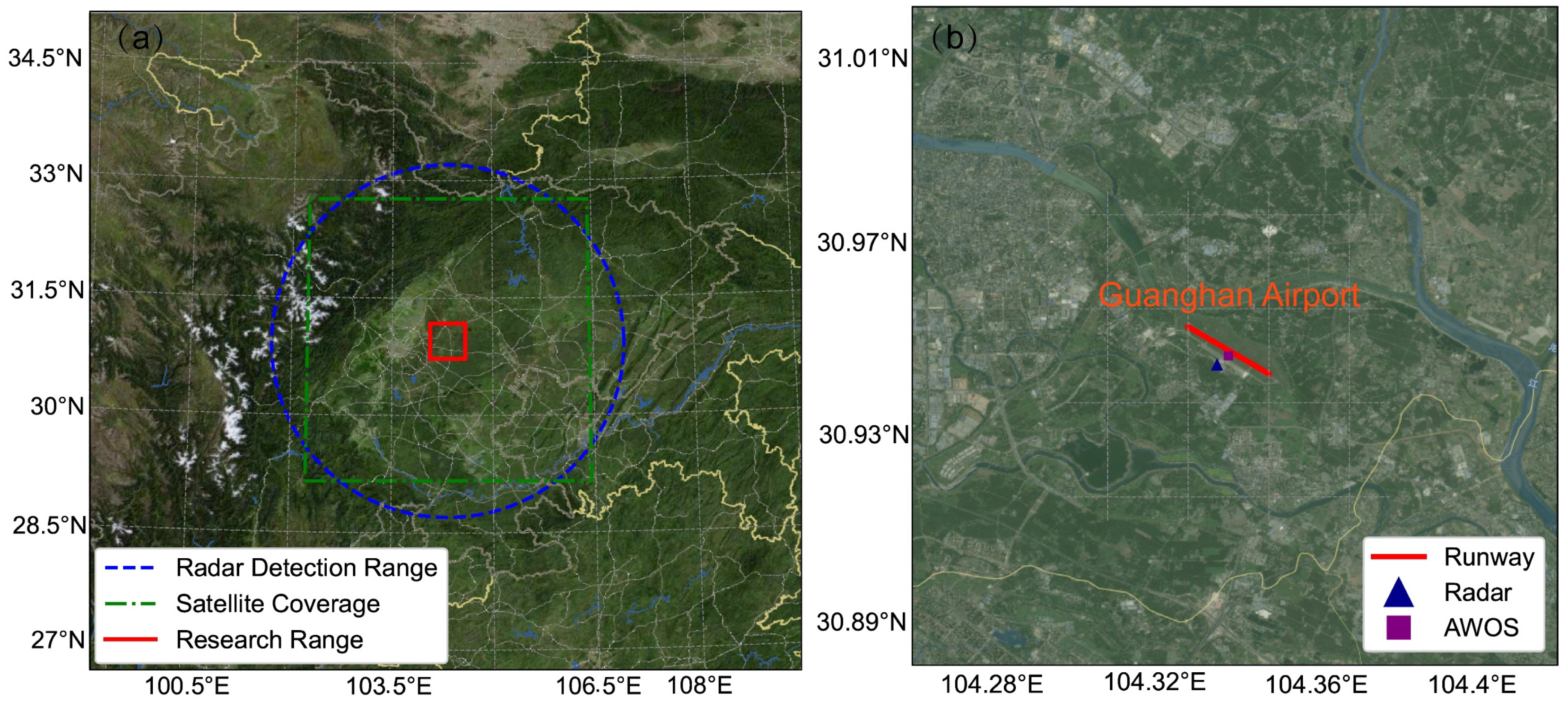
Figure 1. Geographical settings of the study area. (a) Regional overview showing the radar detection range (blue dashed line), cropped satellite coverage (green dash-dotted line), and cropped radar coverage (red solid line) centered at Guanghan Airport. (b) Enlarged view of Guanghan Airport with observation site locations, including the runway (red line), radar starion (blue triangle), ad AWOS station (purple triangle).
Atmosphere 17 00497 g001
Figure 2. An overview of the CNN-ConvLSTM architecture for severe convective weather nowcasting. The three colored branches in the 2D-CNN module (black, yellow and green) corresponded to radar, and optical flow inputs, respectively. In the LSTM mechanism diagram, blue circles represent element-wise operations, and purple circles represent activation functions.
Atmosphere 17 00497 g002
Figure 3. Detailed configuration of the CNN-ConvLSTM model used in this study, where “B” denotes the batch size. Different colors represent different types of data processing operations, and arrows indicate the data flow direction between layers.
Atmosphere 17 00497 g003
Figure 4. Comparison of training dynamics under different learning rates with and without optical flow features. Panels (ac) show training and validation loss curves for the OF model at lr = 0.0001, 0.0005, and 0.001, respectively. Panels (eg) show the corresponding loss curves for the No_OF model. (d) Box plots comparing the Threat Score distributions of the OF model across the three learning rates. (h) Box plots comparing the Threat Score distributions of the No_OF model across the three learning rates. Shaded regions around the training loss (blue) and validation loss (red) curves indicate 95% confidence intervals.
Atmosphere 17 00497 g004
Figure 5. Comparison of Threat Score (TS) performance under different focal weight values (f = 0.6, 0.7, 0.8) for models with and without optical flow (OF) features.
Atmosphere 17 00497 g005
Figure 6. Interactive effects of α (class weights) and γ (focusing parameter). (a) With radar optical flow features, (b) Without radar optical flow features.
Atmosphere 17 00497 g006
Figure 7. Probability distribution histograms of model predictions for severe convective weather types. (ac) Models incorporating optical flow features and (df) models without optical flow features for heavy rainfall, strong winds, and thunderstorms, respectively. Orange and blue bars denote positive and negative samples.
Atmosphere 17 00497 g007
Figure 8. Feature importance comparison for models (a) with and (b) without optical flow features. Error bars represent standard deviations.
Atmosphere 17 00497 g008
Table 1. Data source description.
Data SourceSpatial ResolutionTemporal ResolutionCoverageKey Parameters
Doppler Weather Radar Images125 m/pixel10 min400 × 400 px (~50 × 50 km2)15 elev. angles (0.5–19.5°)
Satellite Cloud Images (Himawari-8)2 km/pixel10 min200 × 200 px
(~400 × 400 km2)
3 IR channels: 2.3, 6.2, 10.4 um
Airport automatic weather station (airport AWS)Point observation at the runway midpoint (30.95° N, 104.34° E)1 min (to 10 min)Single stationTemperature, air pressure, wind direction, wind speed, 3-h/24 h pressure changes, 3-h/24 h temperature changes.
Radar Optical FlowDerived10 minSame as radarMotion vectors (u, v) via TV-L1
Table 2. Definition of Severe Convective Weather for General Aviation Airports.
Type of Severe Convective WeatherDefinition
ThunderstormA group of electrical discharges occurring within, between, or beneath cumulonimbus clouds, characterized by visible lightning and audible thunder. In some cases, thunder may be heard without visible lightning. Additionally, it is identified by the presence of strong radar echoes within a 25 km radius centered on the airport.
Strong windsSurface instantaneous wind speed ≥ 10 m/s occurring more than twice, or an instantaneous wind speed deviation ≥ 5 m/s from the 10 min average wind speed.
Short-term Heavy RainfallPrecipitation intensity that impacts flight takeoff and landing safety, specifically rainfall of moderate or heavier intensity. This is defined as minute-level precipitation ≥ 0.5 mm occurring more than three times.
Table 3. Optimal hyperparameters for models with/without optical flow.
Lrfαγ
OF0.00010.6[0.85,0.95.0.98]5
No_OF0.00010.7[0.85,0.95.0.98]4
Table 4. Performance comparison of models with/without optical flow fields.
Model Accuracy F1_MacroROC_AUCTS
With optical flow0.890.7920.9250.705
Without optical flow0.9040.7190.90.567
Table 5. Confusion matrix and F1 Scores for models with and without optical flow.
Weather TypeModelTNFPFNTPF1
ThunderstormWithout OF38160120.60
With OF41130120.65
Heavy RainfallWithout OF3808200.83
With OF3806320.91
Strong WindWithout OF5401110.15
With OF5400121.00
Disclaimer/Publisher’s Note: The statements, opinions and data contained in all publications are solely those of the individual author(s) and contributor(s) and not of MDPI and/or the editor(s). MDPI and/or the editor(s) disclaim responsibility for any injury to people or property resulting from any ideas, methods, instructions or products referred to in the content.