Long Memory Characteristics of Global Temperature Anomalies (1850–2025)

Abstract

The oceans have absorbed most of the excess heat generated by anthropogenic climate change, yet the temporal structure of this warming remains insufficiently understood. This study analyses global temperature anomaly records from polar, tropical, and hemispheric regions over the period January 1850–October 2025, using fractionally integrated time-series methods to characterize long-range dependence and persistent warming. The results reveal statistically significant long memory across all regions, with particularly high persistence in the tropical Atlantic and the eastern North Pacific, as well as robust warming trends in polar and hemispheric aggregates series. These findings indicate that ocean warming is a structurally persistent process with implications for environmental governance. The strong climatic inertia observed suggests that policy frameworks with short planning horizons may underestimate long-term risks, underscoring the need to incorporate long-memory processes into climate risk assessments and the design of mitigation and adaptation strategies.

1. Introduction

Climate change, caused largely by increased anthropogenic greenhouse gas emissions [1,2,3] not only increases the likelihood of extreme weather events, but also causes rising temperatures, changes in precipitation patterns, sea level rise, and profound changes in the ocean, such as warming and acidification. These effects have repercussions on ecosystems, health, water resources, and human activities, generating greater environmental and socioeconomic risks on a global scale.

Climate models indicate that, even with an immediate and substantial reduction in greenhouse gas emissions, global warming will continue until approximately 2050 due to the inertia of the climate system and the impossibility of suddenly eliminating emission sources [4,5]. However, rapid and deep mitigation would slow and limit this warming, with projections diverging from 2050 onwards depending on the policies implemented. In scenarios with drastic and sustained reductions in carbon dioxide, the global temperature would tend to stabilize, reaching values close to 1.5 °C above pre-industrial levels by the end of the 21st century [6].

According to the annual assessment by the Global Carbon Project [7], the oceans absorb approximately 3.0 Pg C per year, representing about a quarter of total anthropogenic CO₂ emissions. This estimate highlights the essential role of the ocean as a carbon sink, regulating the increase in atmospheric CO₂ and generating direct effects on the chemistry of surface waters [8]. Similarly, one of the most relevant features of climate change is that the oceans are the main reservoir of excess heat, accumulating around 93% of the additional energy retained in the climate system since the mid-20th century [6,9,10]. This inequality in energy absorption makes the ocean a central element in understanding the global heat balance and anticipating the long-term repercussions of global warming.

Recent observations and reconstructions indicate that ocean warming is not limited to the surface but progressively penetrates to depths of hundreds and even thousands of meters within the ocean [11,12]. Global sea surface temperature shows a sustained upward trend [13], although this warming shows marked spatial variability between basins and is particularly intense in the northern hemisphere. The most recent estimates indicate that global surface temperatures have risen by more than 0.4 (±0.02) °C since 1993, confirming a notable acceleration in recent decades [14]. Except for regions linked to the major Pacific, Atlantic, and Southern Ocean current systems, most of the ocean surface is experiencing a clear increase in temperature. It is noteworthy that around 75% of the surface waters in the northern hemisphere are warming at a rate above the global average, compared to approximately 35% in the southern hemisphere, highlighting a pronounced interhemispheric asymmetry in the distribution of ocean warming [8].

Ocean warming is therefore a profoundly regional phenomenon, and the characteristics of thermal change both at the surface and at different depths differ significantly between basins [15,16]. These differences are relevant because they condition local and regional responses of the climate system. Added to this is the variability in the behavior of carbon dioxide between ocean regions; at high latitudes, low temperatures favor the dissolution of CO₂ and its transport to deep layers through convection and currents, making the North Atlantic, the Arctic, and Antarctica crucial carbon sinks. In contrast, in warm waters at low latitudes, the lower solubility of CO₂ and upwelling driven by trade winds facilitate the release of this gas into the atmosphere [8]. Assessing these heterogeneities over a broad time horizon (1850–2025) is essential for understanding the evolution of ocean warming and designing more effective climate policies aimed at its mitigation or attenuation.

From a methodological point of view, the analysis of historical oceanic time series poses particular challenges due to the heterogeneity of sources, changes in measurement practices, and the presence of long-range temporal dependence. To address these characteristics, fractional integration provides an appropriate framework, as they allow for a non-integer differentiation parameter capable of capturing prolonged persistence, and improving the detection of persistent trends. These approaches have a solid theoretical basis [17,18,19] and have been successfully applied to climate and ocean series to analyze memory, trend, and fractional cointegration [20,21,22]. Thus, for example, ref. [23] estimates the differencing parameter using the output of long simulations with a General Circulation Model rather than observations, which allows for the analysis of long-term dynamics over broader time horizons than those available in observational data. Their results provide evidence of long-range dependence in simulated temperature records highlighting that persistence is a relevant feature of climate dynamics when very long time horizons are considered. In this context, although our analysis is based on observational data, the results obtained are consistent with this evidence, suggesting that long memory is a robust characteristic of temperature series in both simulated and observed settings.

From a statistical perspective, determining the degree of long memory is essential for understanding the nature and persistence of climate shocks, as well as for correctly assessing the statistical significance of deterministic trends in the presence of persistent residuals. In this context, this study aims to analyze time series of ocean warming in the Arctic, Antarctic, Atlantic (including the MDR region), eastern-northern Pacific, and northern and southern hemispheres, covering the period from 1850 to 2025. The objective is to characterize long-term trends in the context of persistent data. In particular, by properly estimating the order of integration from a fractional viewpoint, it will permit us to determine potential trends in the data in a much more precise way than under the classical methods based on integer differentiation. Thus, the application of fractional integration techniques will allow us to estimate temporal persistence, detect possible recent ruptures or accelerations, and formally compare thermal dynamics between ocean basins and layers. The aim is to provide quantitative evidence and a robust methodological framework that will contribute to interpreting ocean warming and support projections and mitigation and adaptation policies.

The main contribution of this study lies in the application of fractional integration techniques to a comprehensive set of long-run ocean temperature series within a unified econometric framework. Unlike standard approaches based on short-memory or unit-root models, this methodology allows for a more flexible characterization of persistence, providing additional insights into the temporal dynamics of ocean temperature variability. Beyond this methodological contribution, the study addresses a specific research question: whether persistence patterns and underlying dynamics differ systematically across oceanic regions when analyzed within a unified framework over a long historical period. This approach enables a consistent comparison across climatic regimes and provides additional insight into regional differences in ocean temperature dynamics.

2. Temperatures in the Oceans

The evolution of ocean temperatures in recent decades reveals sustained, accelerated, and global warming affecting both the surface and deep layers of the ocean (up to 2000 m). In fact, in 2023, the total ocean heat content (OHC) reached a historic record of 464 ± 55 ZJ accumulated since 1960. This jump is equivalent to a considerable increase in the energy stored by the oceans, with a net heat gain of 16 ± 10 ZJ compared to 2022 [11].

In 2024, both global sea surface temperature and heat content up to 2000 m reached historic values. In particular, global OHC between 0 and 2000 m in 2024 exceeded that of 2023 by 16 ± 8 ZJ [24]. As for ocean surface temperature, the trend is also clear: between 1982 and 2023, the global average sea surface temperature has increased at a rate of 0.13 ± 0.01 °C per decade. This surface warming is particularly intense in the northern hemisphere, where approximately 75% of the ocean surface is warming at a rate above the global average [8].

The above data confirm that the oceans continue to absorb most of the excess heat derived from the increase in greenhouse gases in the atmosphere. The implications of this evolution are profound and multifaceted. The increasing accumulation of heat in ocean waters drives thermal expansion of the water, contributing to sea level rise. In addition, rising surface and deep temperatures alter stratification, ocean circulation, and heat-atmosphere exchange dynamics, which can modify weather patterns, moisture cycles, extreme weather events, and the distribution of thermal energy in the global climate system.

Ecologically, these changes represent thermal stress for marine ecosystems. They increase the likelihood and frequency of marine heatwaves, with adverse effects on resilience, biodiversity, primary productivity, and species distribution. The biogeochemical functions of the ocean (circulation of nutrients, oxygen, carbon) are also affected, with potential repercussions on fisheries, carbon cycles, and the overall health of the ocean [25]. Recent evidence reveals a consistent, global, and intense change in ocean temperatures, and this systematic warming underscores the urgent need to employ models and methodologies that investigate this issue.

It is important to clarify that the statistical persistence identified in ocean temperature series should not be directly interpreted as physical ocean memory. Instead, it reflects long-range temporal dependence that may arise from the interaction of multiple processes. In particular, large-scale modes of climate variability such as ENSO, PDO, and AMO play a key role in shaping ocean temperature dynamics and may contribute to the observed persistence patterns. Moreover, the combined effects of internal variability and externally forced trends can generate persistence that does not necessarily correspond to a single physical mechanism. Therefore, the results derived from fractional integration methods should be interpreted as statistical evidence of temporal dependence, rather than a direct measure of intrinsic physical inertia in the ocean–climate system.

Over the past decade, the study of ocean warming has made remarkable progress thanks to the increased availability of observational records and improved statistical techniques applied to climate. A particularly influential line of research has been that examining the temporal structure of warming in terms of persistence, a property that has been consistently detected in ocean temperature and heat content series. In this context, several recent studies have documented the presence of long-range dependence in climatological time series, highlighting the relevance of long memory for understanding climate variability and persistence [26,27]. In this context, recent work [8,10,11,13] has shown that ocean warming is not only accelerating but also exhibits an organized temporal signal, with interdecadal coherence and long-range dependence features.

Advances in the analysis of these properties have highlighted the limitations of classical models based on short memory. Statistical studies applied to climate suggest that ARIMA models and other integer differentiation approaches underestimate the persistence of the oceanic system and can lead to errors in trend detection [28,29].

In response to these limitations, fractionally integrated models have taken on a central role. Recent research by [30,31] and others has shown that these models reproduce ocean dynamics more accurately because they allow for a non-integer differentiation parameter that captures long-term dependencies. The benefits of using this methodology become especially relevant when analyzing regions with contrasting thermal behaviors or extensive oceanic series. In the North Atlantic, ref. [32] showed that the presence of multi-year or decadal persistence can significantly influence trend estimates if not modeled appropriately.

Furthermore, attribution studies on North Pacific surface temperature [33] show the growing human footprint on regional warming, emphasizing that surface trends must be interpreted in the context of natural variability, induced warming, and possible ocean memory effects. On the other hand, recent work on global ocean heat content [11,13] confirms that a substantial portion of anthropogenic excess heat accumulates in deep waters, which requires the use of tools sensitive to long-term persistence and dynamics for its correct interpretation.

3. Methodology

We use fractional integration techniques. A process {x(t), t = 0, ±1, …} is said to be integrated of order d, and denoted by I(d) if after d-differences the new process becomes I(0) or integrated of order 0 that is defined as a process with a spectral density function that is positive and bounded. Within the category of I(0) (also named short memory) processes we can include the white noise process, which is an uncorrelated process with zero mean and constant variance. However, this I(0) category also permits (weak) time dependence as in the AutoRegressive Moving Average (ARMA) processes. Using an analytical expression, x(t) is I(d) if:

(1 − L)^d x(t) = u(t),

(1)

where L is the lag operator, i.e., L^kx(t) = x(t − k), d can be any real number, and u(t) is I(0).

Supposing that u(t) is an ARMA(p,q) process, traditionally two models have been considered, the stationary ARMA, corresponding to the case where d = 0 and the nonstationary ARIMA when d = 1. However, values of d constrained between 0 and 1 (or even above 1) can also be considered, noting that the polynomial (1 − L)^d in Equation (1) can be expressed such that for any real d:

$${\left(1-L\right)}^d={\sum }_{j=1}^{\mathrm{\infty }}{\displaystyle \frac{\mathsf{\Gamma }\left(\mathrm{d}-1\right){\left(-L\right)}^j}{\mathsf{\Gamma }\left(\mathrm{d}-\mathrm{j}+1\right)\mathsf{\Gamma }\left(\mathrm{j}+1\right)}},$$

(2)

where Γ is the gamma function, which is defined as $\mathsf{\Gamma }\left(\mathrm{z}\right)={\displaystyle {\int }_0^{\infty }}{t}^{z-1}{e}^{-t}d\left(t\right).$ Alternatively, x(t) in (1) can be expressed in terms of an infinite AR process of the form:

$$x(t)=dx\left(t-1\right)-{\displaystyle \frac{d\left(d-1\right)}{2}}x\left(t-2\right)+{\displaystyle \frac{d\left(d-1\right)\left(d-2\right)}{26}}x\left(t-3\right)+\cdots +u(t)$$

(3)

and thus the differencing parameter d can be interpreted as a measure of the degree of persistence: the higher the value of d is, the greater is the degree of persistence, namely the higher is the association between observations, even if they are far apart in time. The parameter d is also sometimes called the memory parameter.

In the following section, since we are also interested in estimating time trends, we suppose first that x(t) are the errors in a regression model that incorporates an intercept and a linear time trend, such that

y(t) = α + βt + x(t),     t = 1, 2, …,

(4)

where y(t) indicates the original data, and α and β stand for the constant and the coefficient on a linear time trend t, that are both estimated from the data along with the memory parameter d.

Finally, note that long memory is a feature observed in climatological and hydrological data, and is characterized because the spectral density function has a pole or singularity at least one frequency in the spectrum. This feature is satisfied by the I(d) class of models like (1) with d > 0, noting that the spectrum of x(t) in (1) becomes:

$$f\left(\lambda \right)=f\left(\lambda ;\tau \right)={\displaystyle \frac{{\sigma }^2}{2\pi }}{\left|{\displaystyle \frac{1}{1-e^{i\lambda }}}\right|}^{2d}g\left(\lambda ;\tau \right),$$

(5)

where g indicates the spectral part of the short run dynamics and clearly, $f\left(\lambda \right)\to \infty ,\mathrm{a}\mathrm{s}\lambda \to 0^{+}.$ The estimation of the parameters involved in the model, that is, those in Equations (1) and (4) is based on the likelihood function in the frequency domain as stated in [34]. This is a testing procedure that uses the model in (1) and (4), and test the null hypothesis H_o: d = d_o, for any d_o-value in the real line. Thus, it is not constrained to the stationary range, and it allows us to compute confidence bands for the non-rejection values. The functional form of this procedure is detailed in [34] and among its advantages with respect to other procedures, is the fact that it has a standard N(0,1) distribution and is the most efficient method in the Pitman sense against local departures. This procedure has been employed in numerous papers including [20,21,22,26,31], etc.

4. Data

The data used correspond to average temperature anomalies in the Arctic, Antarctic, Mid-Atlantic, Northeast Pacific, and northern and southern hemispheres, obtained from the U.S. National Oceanic and Atmospheric Administration (NOAA) series. These series integrate sea surface and land surface temperature records from various long-term observation sets. The information used has monthly resolution and covers the period from January 1850 to October 2025, corresponding to combined global land and ocean temperature anomalies calculated relative to the climatological average for the period 1901–2000.

The regions selected in this study represent key components of the global ocean system with distinct climatic characteristics. They capture a wide range of ocean dynamics, including polar processes, tropical variability, and large-scale hemispheric behavior. These regions are commonly used in climate literature due to their relevance for global climate dynamics. For instance, the Atlantic MDR is closely linked to tropical variability and hurricane activity, while the Eastern North Pacific is strongly influenced by ENSO-related processes. The Arctic and Antarctic regions are essential for understanding polar amplification and the role of the Southern Ocean in regulating global heat distribution. In addition, the selection is guided by data availability and consistency over the long historical period analyzed (1850–2025), ensuring comparability across regions.

Table 1. Descriptive statistics for the series.

Series	Maximum (Peak)	Minimum (Trough)	Mean (Average)	Standard Deviation
Arctic	+5.130 °C in February 2025	−3.710 °C in February 1979	+0.100 °C	1.187 °C
Antarctic	+2.220 °C in August 1996	−1.630 °C in August 1932	+0.044 °C	0.434 °C
Atlantic MDR	+1.840 °C in May 2024	−1.090 °C in June 1861	+0.099 °C	0.459 °C
East North Pacific	+1.790 °C in October 2015	−1.880 °C in December 1946	+0.053 °C	0.481 °C
Northern Hem.	+2.020 °C in November 2023	−1.050 °C in December 1916	+0.079 °C	0.489 °C
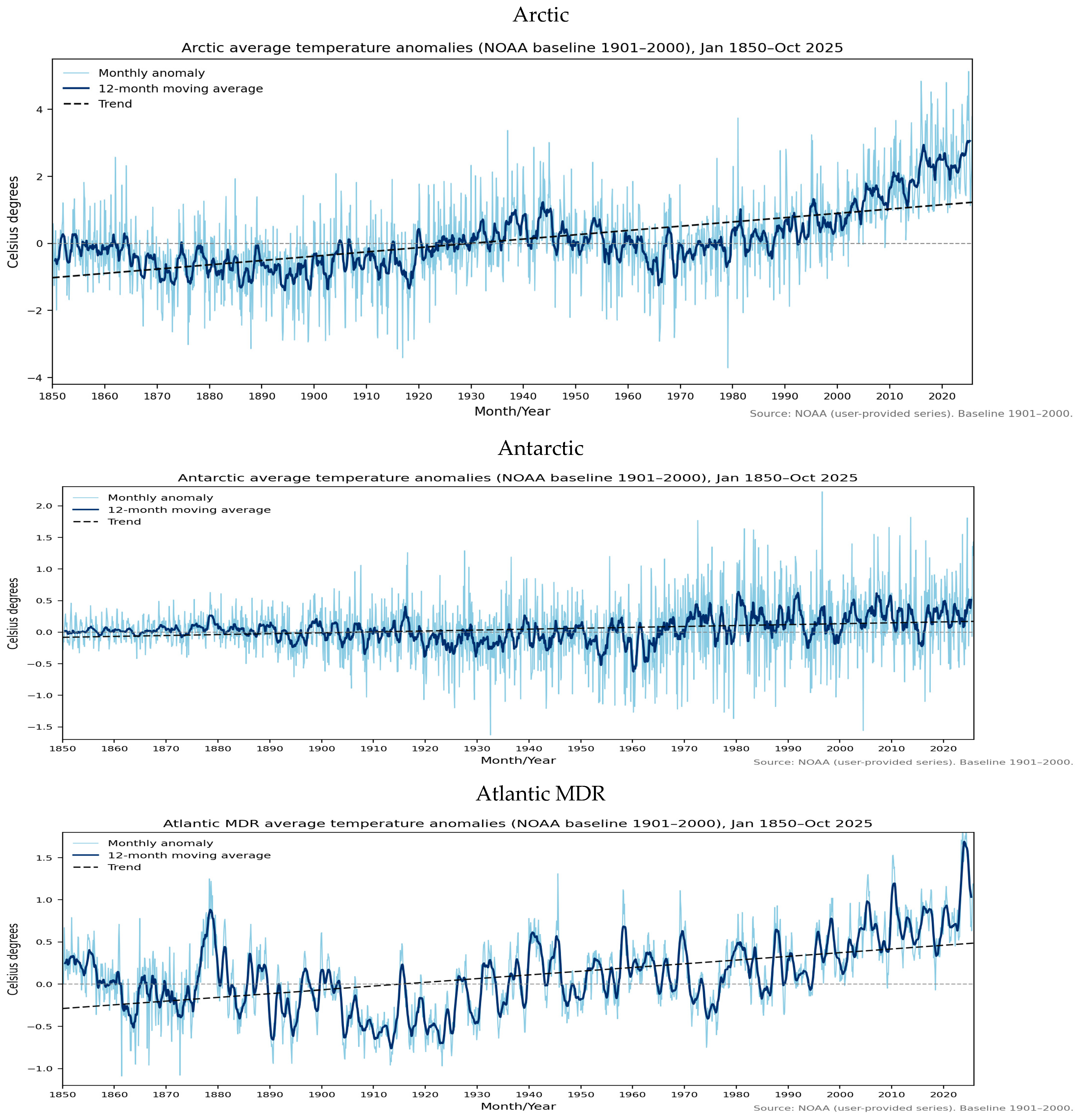
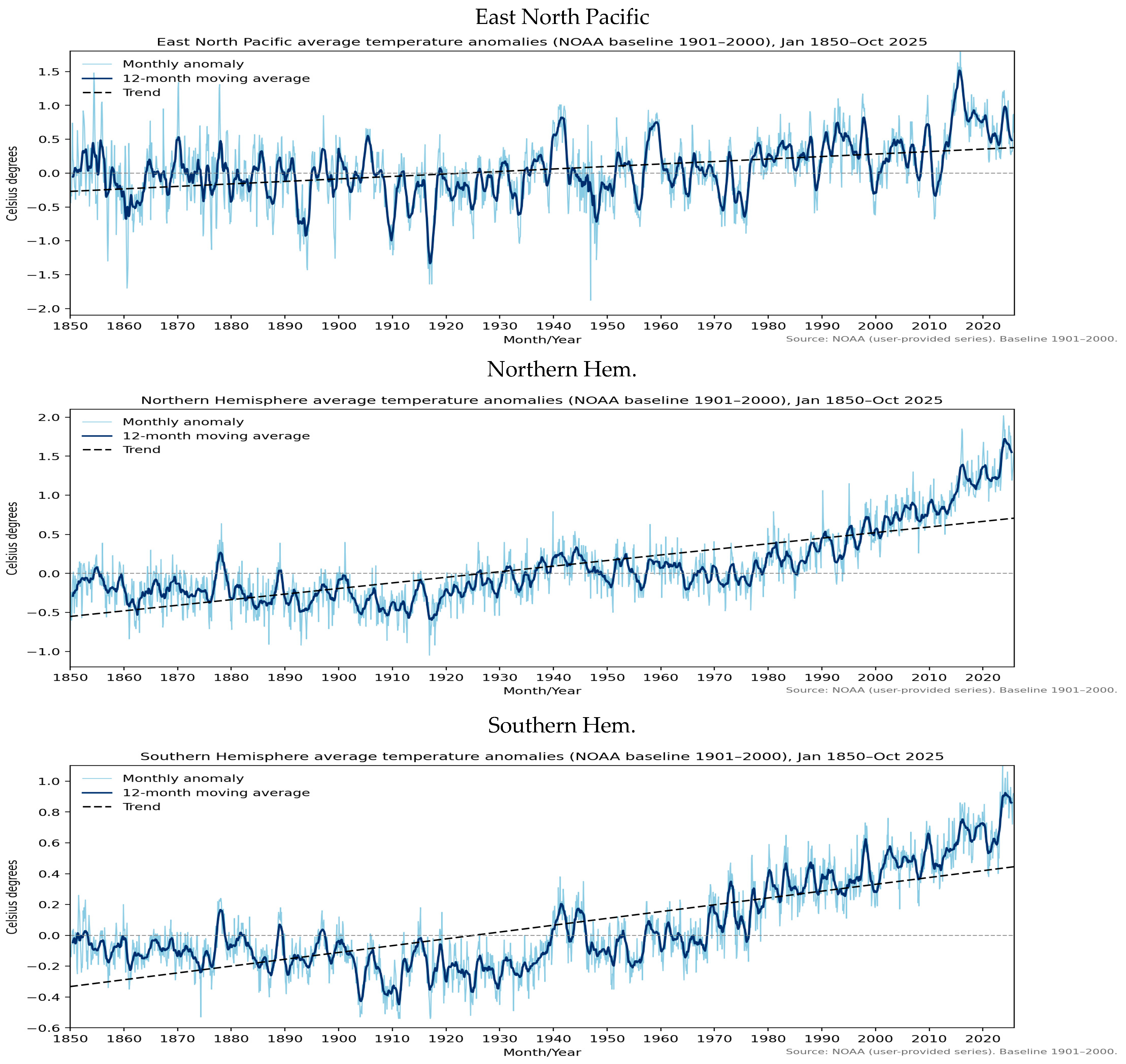
Southern Hem.	+1.100 °C in September 2023	−0.540 °C in March 1911	+0.056 °C	0.305 °C

summarizes the descriptive statistics of the temperature anomaly series for the period 1850–2025, revealing marked spatial heterogeneity in both variability and extreme values. The Arctic clearly stands out as having the greatest thermal amplitude and dispersion, with a maximum of +5.13 °C (February 2025) and a minimum of −3.71 °C (February 1979), as well as the highest standard deviation of all series (1.187 °C), reflecting its high sensitivity to external forcings and the polar amplification mechanism associated with ice-albedo feedbacks and changes in ocean stratification (IPCC, 2021 [6]; Caporale et al., 2024 [20]). In contrast, Antarctica shows considerably more moderate anomalies with a temperature range between −1.63 °C (August 1932) and +2.22 °C (August 1996) and a significantly lower standard deviation (0.434 °C), which is consistent with the buffering effect of the Southern Ocean and the stabilizing role of its circumpolar circulation, which limits heat transfer to the surface [6].

The tropical and subtropical basins, represented by the Atlantic in the MDR region and the eastern North Pacific, exhibit intermediate variability with standard deviations of 0.459 °C and 0.481 °C, respectively. However, both regions show positive mean anomalies (+0.099 °C in the MDR Atlantic and +0.053 °C in the eastern North Pacific), indicating sustained long-term warming driven by ocean-atmosphere coupling and the continuous accumulation of anthropogenic heat in the upper ocean layers [8,10,11].

Finally, the hemispheres smooth out some of the regional variability although they show clear asymmetry. The northern hemisphere has greater dispersion (standard deviation of 0.489 °C) and more pronounced extremes with a maximum of +2.02 °C (November 2023) compared to the southern hemisphere, which has less variability (0.305 °C) and extreme values ranging from −0.54 °C to +1.10 °C. This asymmetry is consistent with the unequal distribution between continental and oceanic masses and with the greater intensity of anthropogenic forcing in the northern hemisphere [21].

Figure 1 illustrates the temporal evolution of the temperature anomalies in the different regions analyzed. All series show a consistent and sustained long-term warming signal, with a clear intensification since the late 20th century. The Arctic shows the most pronounced acceleration in recent decades, in line with polar amplification processes, while the hemispheric series reveal persistent and spatially consistent warming on a global scale. Although short-term fluctuations and transient cooling episodes are observed, especially in the mid-latitude oceans, these variations occur around a progressively higher average level, indicating that anthropogenic-forced warming clearly dominates over the internal variability of the climate system.

Beyond the growing trend, the temporal structure of the series unequivocally suggests the presence of long-range dependence. The observed persistence implies that thermal anomalies do not dissipate quickly but maintain a significant correlation even at long time lags. This behavior is consistent with previous evidence documenting the existence of long memory in ocean temperature series [11,28,29].

5. Empirical Results

Table 2. Estimates of d under three scenarios for the deterministic terms.

Series	With No Regressors	With an Intercept	With an Intercept and a Linear Time Trend
Arctic	0.345 (0.323, 0.369)	0.345 (0.323, 0.369)	0.321 (0.296, 0.349)
Antarctic	0.196 (0.170, 0.223)	0.197 (0.171, 0.224)	0.189 (0.162, 0.227)
Atlantic MDR	0.844 (0.803, 0.889)	0.844 (0.803, 0.891)	0.845 (0.803, 0.891)
East North Pacific	0.758 (0.716, 0.808)	0.759 (0.717, 0.805)	0.759 (0.717, 0.807)
Northern Hem.	0.513 (0.491, 0.538)	0.510 (0.488, 0.534)	0.499 (0.474, 0.526)
Southern Hem.	0.598 (0.572, 0.629)	0.597 (0.571, 0.627)	0.591 (0.563, 0.623)

The values refer to the estimates of the differencing parameter d. In parenthesis, 95% confidence bands. In bold the selected specification in relation with the deterministic term for each series.

displays the estimates of d (and their associated 95% confidence bands) in a model given by Equations (1) and (4); however, and based on the monthly nature of the data, we also suppose that u(t) is a seasonal (monthly) AR(1) process of the form:

u(t) = ρ u(t − 12) + ε(t),

(6)

where ε(t) is now a white noise process. Thus, the model examined is the following one,

$$\mathrm{y}\left(\mathrm{t}\right)=\mathsf{\alpha }+\mathsf{\beta }\mathrm{t}+\mathrm{x}\left(\mathrm{t}\right),(1-L{)}^{d}x\left(t\right)=u\left(t\right),u\left(t\right)=\rho u\left(t-12\right)+\epsilon \left(t\right)$$

(7)

for t = 1, 2, …, T. Note that the deterministic structure for the time trend is jointly estimated with the fractional differencing equation, such that, taking together the first two equalities in (7) it becomes:

$$y^{*}\left(\mathrm{t}\right)=\mathsf{\alpha }{1}^{*}\left(\mathrm{t}\right)+\mathsf{\beta }{t}^{*}\left(\mathrm{t}\right)+\mathrm{u}\left(\mathrm{t}\right),$$

(8)

where $y^{*}\left(\mathrm{t}\right)=(1-L{)}^{d}y\left(t\right)$; $1^{*}\left(\mathrm{t}\right)=(1-L{)}^{d}1$; and $t^{*}\left(\mathrm{t}\right)=(1-L{)}^{d}t$, and u(t) is I(0) by construction. Then, for example, if d = 1 the time trend disappears, and, if u(t) is a white noise process, y(t) becomes a random walk process with a drift, i.e., y$\left(\mathrm{t}\right)=\mathsf{\alpha }+\mathrm{u}\left(\mathrm{t}\right),\mathrm{t}=1,2,\dots$.

Column 2 in Table 2 reports the estimates of d under the assumption that there are no deterministic terms, i.e., y(t) = x(t); column 3 displays the results under the assumption that the model contains an intercept, while the last column allows for both an intercept (α) and a linear trend (β). We have marked in bold in the table the selected specification for each series, this selection being made based on the statistical significancy of these deterministic terms. The first observed thing is that the time trend is required in four out of the six series, (all except Atlantic MDR and East North Pacific).

Table 3. Estimated parameter in the selected models.

Series	Diff. Parameter d (95% Conf. Band)	Intercept (t-Value)	Time Trend (t-Value)	Seasonal Coff.
Arctic	0.321 (0.296, 0.349)	−0.81933 (−3.56)	0.00108 (5.74)	0.057
Antarctic	0.189 (0.162, 0.227)	−0.07349 (−2.31)	0.00012 (2.84)	0.038
Atlantic MDR	0.844 (0.803, 0.889)	---	---	0.018
East North Pacific	0.758 (0.716, 0.808)	---	---	−0.040
Northern Hem.	0.499 (0.474, 0.526)	−0.43250 (−4.39)	0.00066 (6.09)	0.100
Southern Hem.	0.591 (0.563, 0.623)	−0.12294 (−1.81)	0.00035 (3.30)	0.033

The values in parenthesis in column 2 indicate the 95% confidence interval of the non-rejection values of d; those in columns 3 and 4 are the t-values of the coefficients of the intercept and the time trend respectively.

displays the estimated coefficients for the selected model for each series. The results provide strong evidence that ocean temperature dynamics are governed by long-term dependence and persistent warming in all regions analyzed. In fact, the estimated fractional differentiation parameter (d) is positive and statistically significant in all cases, indicating that long-term memory is a structural feature of ocean thermal variability.

However, this persistence should be interpreted with caution from a physical perspective. The statistical evidence of long-range dependence may reflect not only intrinsic ocean processes but also the influence of large-scale modes of variability and externally forced trends. In particular, the interaction between internal variability and anthropogenic forcing may generate persistence patterns that do not necessarily correspond to a single physical mechanism.

The greatest persistence is observed in tropical and subtropical basins. Atlantic (MDR) has d values close to 0.844, and the Eastern North Pacific has values close to 0.76, implying highly persistent processes in which temperature anomalies decrease very slowly over time. The relatively high persistence observed in these regions may be associated with the influence of large-scale climate variability modes such as ENSO, PDO, and AMO, which play a key role in modulating ocean temperature dynamics through ocean–atmosphere interactions. However, for these two cases, the time trend coefficient was found to be statistically insignificant. The hemispheric series show equally strong persistence, with d ≈ 0.50 in the Northern Hemisphere and d ≈ 0.60 in the Southern Hemisphere, confirming that long-term memory is a systemic property of the global ocean. The Arctic shows intermediate persistence (d ≈ 0.32), while Antarctica has the lowest persistence (d ≈ 0.19), although still significantly different from zero. These differences can be more explicitly linked to well-established physical mechanisms, including Arctic amplification processes in the Northern Hemisphere and the stabilizing role of the Southern Ocean and its circumpolar circulation in the Southern Hemisphere.

The selected models reveal significant positive linear trends, especially in the Arctic, where the warming signal is most intense (trend coefficient = 0.00108; t-value = 5.74), consistent with amplification processes (Caporale et al., 2025) [20]. Comparable positive trends are observed on a hemispheric scale, reinforcing the existence of a sustained signal of global ocean warming. Lower trends are detected for the Antarctic and Southern hemisphere data. The seasonal effect seems irrelevant in the six series examined, and performing seasonal unit root tests [35,36], the results reject the null of nonstationary seasonality in all cases considered.

As an additional checking on the long memory feature of the data, we replace the linear structure in the first equality in (7) by a non-linear one and based on the Chebyshev polynomials in time. Thus, the new model examined is:

$$y\left(t\right)={\sum }_{i=0}^m{\theta }_i{P}_{iT}\left(t\right)+x\left(t\right),(1-L{)}^{d}x\left(t\right)=u\left(t\right),u\left(t\right)=\rho u\left(t-12\right)+\epsilon \left(t\right)$$

(9)

where m denotes the number of coefficients of the Chebyshev polynomials, and P_i,T(t) is defined as $P_{0,T}\left(t\right)=1,$ and $P_{i,T}\left(t\right)=\sqrt{2}\mathit{cos}\left({\displaystyle \frac{i\pi \left(t-0.5\right)}{T}}\right).$

In this context, if m = 0 the model includes an intercept, while for m > 0, the model becomes non-linear—the higher m is the less linear the model becomes. (See [37,38] for a description of these polynomials). For the estimation, we rely here on a procedure developed in [39]. The results are reported across

Table 4. Estimated parameter in the non-linear models.

Series	d (95% Band)	θ1 (t-Value)	θ2 (t-Value)	θ3 (t-Value)	θ4 (t-Value)
Arctic	0.319 (0.285, 0.358)	0.1854 (1.13)	−0.6345 (−5.60)	0.3300 (3.31)	−0.2043 (−2.27)
Antarctic	0.178 (0.132, 0.212)	0.0434 (1.43)	−0.0749 (−3.04)	0.0899 (3.92)	−0.0189 (−0.87)
Atlantic MDR	0.844 (0.803, 0.892)	0.0907 (0.06)	−0.2637 (−0.33)	0.1862 (0.39)	−0.0030 (−0.09)
East North Pacific	0.760 (0.712, 0.813)	−0.1124 (−0.10)	−0.2310 (−0.35)	0.1180 (0.28)	−0.0376 (−0.12)
Northern Hem.	0.498 (0.465, 0.534)	0.0887 (0.76)	−0.3961 (−5.65)	0.2008 (3.54)	−0.1055 (−2.21)
Southern Hem.	0.589 (0.542, 0.623)	0.0658 (0.56)	−0.2383 (−3.45)	0.1616 (3.06)	−0.0312 (−0.73)

The values in parenthesis in column 2 indicate the 95% confidence interval of the non-rejection values of d; those in columns 3–6 are the t-values of the coefficients of the intercept and the time trend respectively. In bold significancy at 5% level.

.

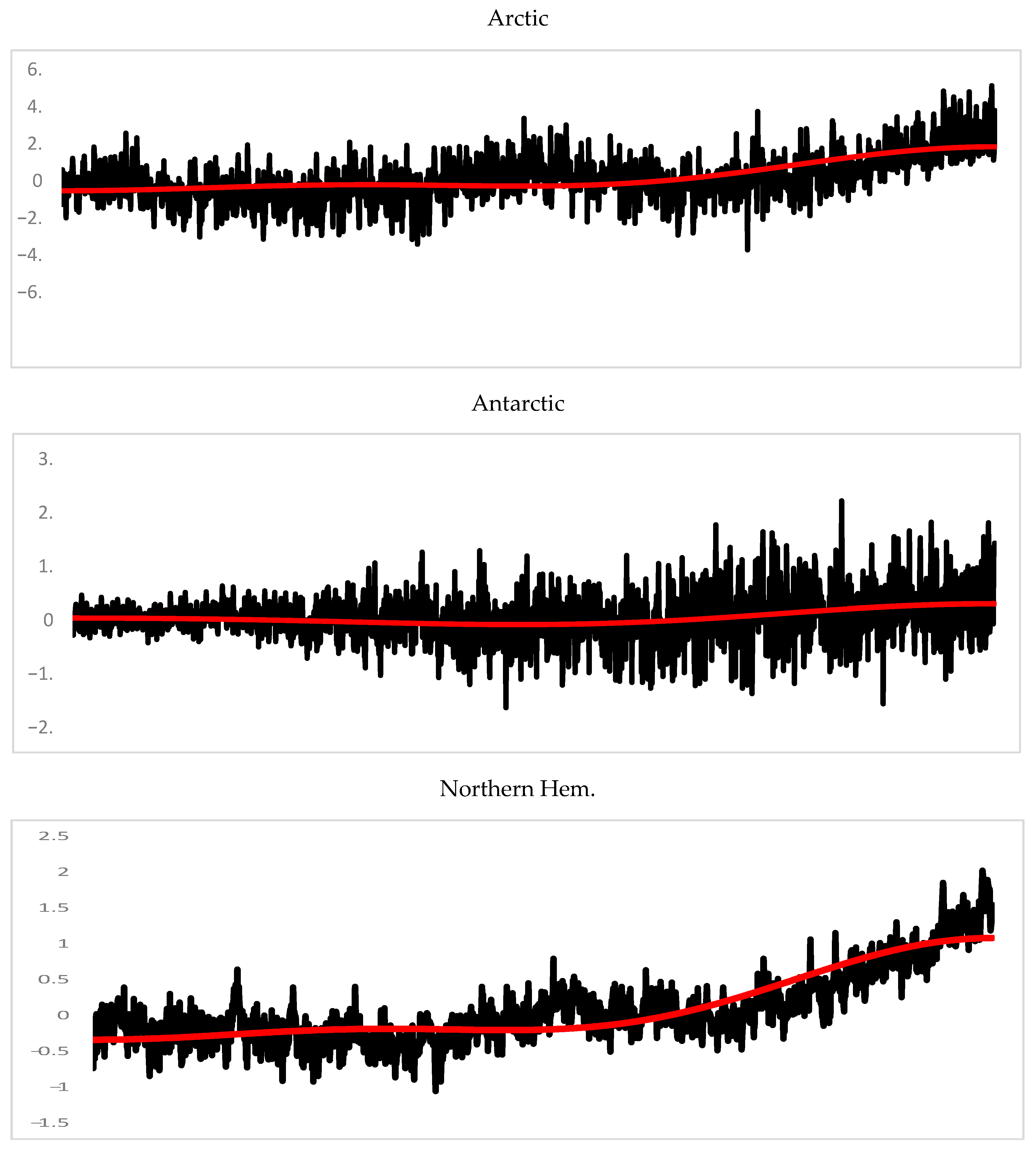
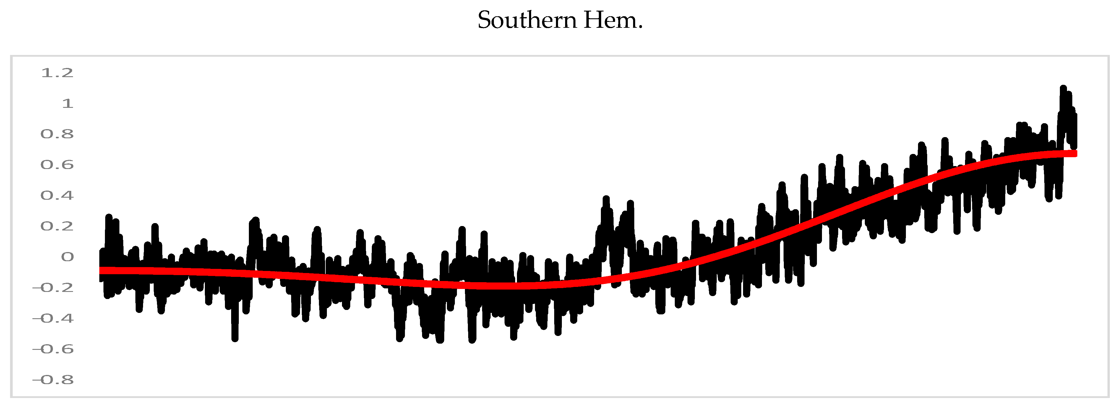
The first thing we observe in Table 4 is that the estimates of d are almost identical to those reported in Table 3 for the linear case; however, some of the non-linear Chebyshev coefficients results statistically significant, particularly for Arctic and Northern Hemisphere but also for Antarctic and Southern Hemisphere. Figure 2 displays the estimated trends for each of the series with significant trends. It can be seen that it produces a smoother change in the trends compared with structural breaks and other approaches.

These results have relevant implications for the interpretation of long-term climate dynamics. The presence of long-term memory implies that the ocean-climate system exhibits strong inertia, such that the impacts of greenhouse gas emissions persist for decades even under scenarios of rapid mitigation.

6. Discussion and Conclusions

This study provides solid and robust evidence that ocean temperature anomalies are governed simultaneously by highly persistent stochastic processes and by long-term deterministic warming. By applying fractional integration techniques to regional and hemispheric series spanning more than 170 years (1850–2025), the results suggest that long-range dependence is a robust statistical feature of global temperature variability. However, this should not be interpreted as direct evidence of intrinsic physical memory alone, but rather as an emergent property that may arise from the interaction of multiple processes, including internal variability, external forcing, and ocean–atmosphere coupling.

From a methodological perspective, this study contributes to the literature by providing a unified fractional integration framework applied to long-term ocean temperature series, allowing for a consistent comparison across regions and a more flexible modeling of persistence.

The results reveal significant regional differences in the degree of persistence. Tropical and subtropical basins, particularly the Atlantic in the MDR region and the eastern North Pacific, have very high memory parameter values, indicating that thermal anomalies in these areas dissipate very slowly. This behavior is consistent with strong ocean-atmosphere coupling, large-scale circulation patterns, and the progressive accumulation of anthropogenic heat in the upper layers of the ocean. In contrast, the polar regions show less persistence, although statistically significant, with the Arctic being more persistent than Antarctica. These differences are consistent with well-known physical mechanisms such as polar amplification in the northern hemisphere and the stabilizing role of the Southern Ocean and its circumpolar circulation in the southern hemisphere. It should be emphasized that these interpretations do not imply a one-to-one correspondence between the estimated statistical persistence and a single physical mechanism but rather reflect the combined influence of multiple interacting processes within the ocean–climate system.

In addition, statistically significant positive linear trends are detected in most series, especially in the Arctic and in hemispheric aggregates. The coexistence of long memory and deterministic trends implies that ocean warming is a cumulative and highly inertial process. In this context, transient cooling episodes or phases of apparent stabilization should not be interpreted as a reversal of warming but as short-term fluctuations around a persistent warming trajectory.

From a methodological point of view, the results highlight the limitations of traditional short-memory models in the analysis of climate series. Ignoring long-range temporal dependence can lead to a systematic underestimation of persistence, biased inferences about trends, and misidentification of structural breaks. In this sense, fractional integration models provide a more appropriate framework for capturing the real dynamics of the ocean-climate system by allowing simultaneous modeling of gradual trends and prolonged persistence over time. The long memory feature observed in the data may also be due to the aggregation of intrinsic forces of heterogeneous nature; in fact, this has been claimed to be a classical argument from a statistical viewpoint: refs. [17,40] argued that the aggregation of heterogenous short memory processes may induce a long memory component in the data. In addition, it cannot be ruled out that the estimated persistence reflects, at least partially, what is known as pseudo long memory, associated with structural changes, nonlinearities or persistent external forcing. These are issues that will be investigated in future papers.

The implications of these findings for environmental and climate policy are noteworthy. Thus, the inertia detected in ocean temperatures might indicate that the effects of greenhouse gas emissions are likely to persist over long time horizons, even under mitigation scenarios. This highlights the importance of considering persistence and delayed responses when interpreting climate dynamics.

Considering the ocean as a heat reservoir with high persistence implies recognizing that the benefits of mitigation policies will not be immediate but will be crucial in limiting cumulative future risks such as sea level rise, intensification of marine heatwaves, and impacts on biodiversity and ocean-dependent economic activities.

Future research could extend this approach to deep-water temperature data and explore fractional cointegration relationships between ocean basins, with the aim of deepening our integrated understanding of the global ocean-climate system. In this context, distinguishing between statistical persistence and physical mechanisms remains a challenging task in climate time series analysis. Future research should aim to integrate statistical approaches with physically based models in order to better disentangle the contributions of internal variability, external forcing, and structural dynamics in the ocean–climate system. Therefore, the results should be interpreted as robust evidence of persistent temporal dependence in the analyzed series, without necessarily implying the existence of intrinsic long memory in a strict physical sense.