Article

A Paleoclimate-Compatible Framework for Modeling Lightning-Caused Ignition Probability in Alaska

by
Charlotte Uden
1,*,
Patrick J. Clemins
2,3 and
Brian Beckage
1,3,4,5,*
1
Department of Plant Biology, University of Vermont, Burlington, VT 05405, USA
2
Vermont EPSCoR, University of Vermont, Burlington, VT 05405, USA
3
Department of Computer Science, University of Vermont, Burlington, VT 05405, USA
4
Gund Institute for Environment, University of Vermont, Burlington, VT 05405, USA
5
Vermont Complex Systems Institute, University of Vermont, Burlington, VT 05405, USA
*
Authors to whom correspondence should be addressed.
Atmosphere 2026, 17(5), 490; https://doi.org/10.3390/atmos17050490
Submission received: 24 March 2026 / Revised: 25 April 2026 / Accepted: 29 April 2026 / Published: 11 May 2026
(This article belongs to the Section Climatology)

Abstract

Understanding the role of historical lightning-driven fire regimes in shaping terrestrial ecosystems and carbon cycles requires reconstructing fire from data beyond the instrumental record. Previous efforts have relied on paleo proxies, such as charcoal records, but these approaches are limited by their coarse spatial extent. Alternatively, process-based modeling offers a spatially continuous pathway for simulating lightning-caused fire regimes. However, existing lightning prediction models use upper-atmospheric variables, such as convective available potential energy (CAPE), that are not available in paleoclimate reconstructions, limiting their use beyond the instrumental period. Here, we develop a probabilistic framework for simulating lightning-caused fire ignitions that (1) relies on variables available in paleo reconstructions (near-surface climate, fuel moisture, and land cover) and (2) decomposes lightning-caused fire occurrence into two components: lightning strike rate and lightning ignition efficiency. Both components were trained on modern observational data for Alaska during 2002–2011, and then combined in a Bernoulli model to estimate daily fire probability. Near-surface climate predictors captured spatial and temporal variability in lightning activity with performance comparable to CAPE-based models, and ignition efficiency models showed strong discrimination between fire-causing and non-fire-causing strikes. Despite overestimation under high-risk conditions, the Bernoulli model demonstrated strong discriminatory skill (ROC AUC = 0.894), effectively ranking fire risk across space and time. By explicitly separating lightning occurrence from ignition efficiency and relying on variables available in paleo reconstructions, this approach provides a transferable framework for simulations of historical lightning-fire regimes.

1. Introduction

Wildfires play an important role in ecosystem disturbance regimes, vegetation dynamics, and carbon cycling. Lightning-caused wildfires account for a disproportionately high fraction of the total area burned in many fire-prone regions [1,2]. This is in part due to their association with holdover fires that can smolder for days before detection [3] with longer holdover durations in boreal forests [4,5]. Furthermore, lightning-caused fires respond to climatic and environmental drivers that differ from those of anthropogenic ignitions [6,7]. In Alaska, lightning-caused fires dominate area burned in part because fire management systems allow fires in remote regions to burn with minimal suppression. This corresponds to roughly two-thirds of interior Alaska [8]. Human-caused fires, however, tend to occur near communities and roads where aggressive suppression keeps them small [9,10]. This Alaska-specific fire management approach means that lightning- and human-caused fires behave in distinct ways, emphasizing the need for a targeted approach to modeling lightning-caused ignition. In recent decades, increasing lightning frequency in boreal North America (including Alaska) has driven a rise in fire occurrence [11], and this trend is expected to continue under future climate projections [12].
Reconstructing historical lightning-driven fire regimes offers a pathway for understanding future regime shifts by establishing long-term baselines for climate, fire, and ecosystem interactions. Previous approaches have estimated past fire regimes from charcoal and ice core records [13,14,15,16,17]. However, these proxies are limited in their spatial extent because charcoal deposition declines sharply with distance from a fire. That is, sediment records primarily capture fire activity in the immediate vicinity of a lake [18]. Process-based modeling offers a spatially continuous complement to these proxy-based approaches. By coupling paleoclimate reconstructions with lightning and fire prediction models, fire dynamics can be simulated across centuries or millennia. Before this is possible, however, two limitations must be addressed.
First, most models designed to predict climate-driven changes to lightning rely on atmospheric variables that are unavailable in paleoclimate reconstructions [19,20,21]. Examples include convective available potential energy (CAPE) [22,23,24], column saturation level, lifting condensation level [22], cloud top height, updraft intensity, cold cloud depth [25,26], and geopotential height [27]. Reliance on upper-atmospheric variables is also evident in Alaska-specific models: Bieniek et al. [28] identify convective precipitation as an important predictor and Chen et al. [29] apply CAPE. Recent work from Uden et al. [30] demonstrated that lightning strike rates can be predicted using near-surface variables with comparable accuracy to CAPE-based approaches, providing a viable pathway for paleo-compatible data.
Second, existing lightning-fire parameterizations for boreal North America rarely represent both lightning occurrence and ignition efficiency as independent climate-driven processes. Several studies have modeled fire from lightning occurrence, climate, fuel data, or landscape characteristics, but omit climate-driven changes to lightning [31,32,33]. Other work simulates lightning from climate but does not incorporate ignition efficiency [11]. Neither approach captures the joint conditions required for a fire: an ignition source (lightning) and the effectiveness of the source to result in combustion (ignition efficiency). An exception is Hessilt et al. [12], who use climate-driven simulations of lightning frequencies and ignition efficiency probabilities to estimate future lightning-caused fire counts for boreal North America. Separating these processes preserves interpretability and allows climate signals to differ across lightning occurrence and ignition.
Here, our modeling approach is motivated by a specific paleo application: driving lightning-caused fire predictions using last-millennium climate reconstruction at daily resolution [34,35], and last-Holocene estimates of vegetation cover [36,37,38]. While other paleoclimate products exist, for example, CHELSA-TraCE21k [39] provides global temperature and precipitation coverage at 100-year timestep over the last 21,000 years, their coarser temporal resolution and limited variable availability are not compatible with the framework developed here. This work therefore constitutes a foundational step in reconstructing past lightning-caused fire regimes: developing and validating a modeling framework against modern observational data for Alaska. Our approach allows for future studies to apply these models to reconstruct last millennium estimates of fire and vegetation dynamics beyond traditional paleo fire proxies [40].
With these motivations in mind, we develop a probabilistic modeling framework for lightning-caused fire designed for application in paleoclimate contexts. Specifically, we decompose lightning-caused fire probability into two interacting components: lightning strike rate and lightning ignition efficiency. Both components are trained using predictor variables available in paleoclimate datasets, including near-surface climate variables, fuel moisture indices, and land cover for Alaska, 2002–2018. We then combine these processes into a Bernoulli trial that accounts for both an ignition source (lightning strike rate) and the probability of ignition given a strike (ignition efficiency) to estimate the probability of at least one lightning-caused fire within a given gridcell and day. This approach provides a transferable, probability-based pathway for applying paleoclimate data to reconstruct historical lightning–fire regimes.

2. Materials and Methods

2.1. Data

2.1.1. Lightning

Lightning strike data, including location and time, were obtained from the Alaska Lightning Detection Network (ALDN), maintained by the Alaska Fire Service (AFS) [41,42]. We used two datasets: an earlier dataset (2002–2011) and a newer dataset (2012–2018). From 2002 to 2011, lightning was detected using an impact-based system that reported cloud-to-ground lightning primarily as flashes. During this period, changes in sensor technology, processing software, and network configuration resulted in variable detection efficiency and relatively coarse spatial accuracy, particularly in remote regions of Alaska. As a result, this dataset is characterized by lower positional accuracy. Beginning in 2012, the ALDN transitioned to a time-of-arrival (TOA)-based system. The TOA system records individual strokes and includes cloud-to-ground strikes. Due to differences in stroke versus flash reporting, expanded sensor coverage, and improved detection range, the AFS reports detecting ~2.25 times more lightning events relative to the earlier systems; there are 1,882,857 strikes in the earlier dataset and 1,784,663 strikes in the later dataset. Due to these differences in detection methods and accuracy, we train and test our models on each period separately.
While the models developed in this study are applied to the entire state of Alaska, it should be noted that sensors are heterogeneously spaced [28], making detection efficiency lower in remote areas far from sensors, particularly for the pre-2012 data. This may introduce spatial bias in lightning observations, for example, gridcells located in southeastern Alaska.

2.1.2. Wildfires

Wildfire ignition data were obtained from the Alaska–Yukon–Northwest Territories Fire Emissions Database (AKFED), version 2, archived at the Oak Ridge National Laboratory Distributed Active Archive Center [43]. AKFED provides information on wildfire occurrence across boreal North America from 2002 onward. Fire ignition locations and dates are derived using a combination of large fire perimeter records and satellite-based fire detections from MODIS. Ignition timing is estimated to within approximately one day, and ignitions are identified at spatial resolutions ranging from 500 m to 1 km, depending on whether a fire is detected from a single pixel or multiple adjacent detections. When multiple active fire detections occur simultaneously, the ignition location is defined as the centroid of the detected pixels.

2.1.3. Climate and Fuel Moisture

Climate predictors were downloaded from the Copernicus Climate Change Service. We obtained hourly ERA5 reanalysis data on a 0.25° × 0.25° grid for summer months (June–August) from 2002 to 2018 [44]. The raw variables include CAPE, 2 m air temperature, 2 m dewpoint temperature, total precipitation, 10 m wind speed, surface downward shortwave radiation, and surface pressure (Figure 1a–f). After aggregating to daily means (and daily sums for precipitation), temperature and dewpoint temperature were converted to Celsius and used to calculate relative humidity. The product of CAPE and precipitation was also calculated at the daily scale. We also computed the Canadian Forest Fire Danger Rating System indices following Van Wagner and Pickett [45] from the ERA5 data. These include daily fine fuel moisture code (FFMC), duff moisture code (DMC), and drought code (DC) (Figure 1g–i).

2.1.4. Land Cover

We used land cover data from the North American Land Change Monitoring System (NALCMS) to derive vegetation cover predictors [46]. The NALCMS products provide land cover classification across North America using a standard 19-class legend based on the Land Cover Classification System (LCCS) of the Food and Agriculture Organization of the United States. Four timesteps were used: 2005, 2010, 2015, and 2020. For the years 2005 and 2010, land cover maps are available at 250 m spatial resolution using MODIS satellite imagery. For the 2015 and 2020 datasets, newer generation NALCMS products were produced at 30 m spatial resolution using Landsat multispectral satellite imagery.
For downstream paleo applications of our models, we reclassified the data from 19 classes to three broad cover types consistent with paleo reconstructions of land cover (REVEALS; [36,37,38]). These include conifer (representing temperate or sub-polar needleleaf forests and sub-polar taiga needleleaf forest), broadleaf (tropical/sub-tropical and temperate/sub-polar broadleaf forests), and unforested/open land (shrubland, grassland, polar dwarf vegetation, wetland, barren, and snow/ice). Classes corresponding to cropland, urban land, water, and other non-natural surfaces were excluded. Mixed forest was allocated proportionally into the conifer and broadleaf categories based on the relative prevalence of pure conifer versus broadleaf forest within a gridcell. To match the land cover data to the ERA5 climate and fuel moisture grid, we assigned each land cover pixel to the nearest ERA5 gridcell. Within each ERA5 gridcell, the sum of each reclassified category (conifer, broadleaf, and unforested/open land) was divided by the number of NALCMS pixels so that each cover type is a proportion that sums to 1 (Figure 1j–l). This aligns modern land cover data with available paleo land cover reconstructions.

2.2. Model Definitions

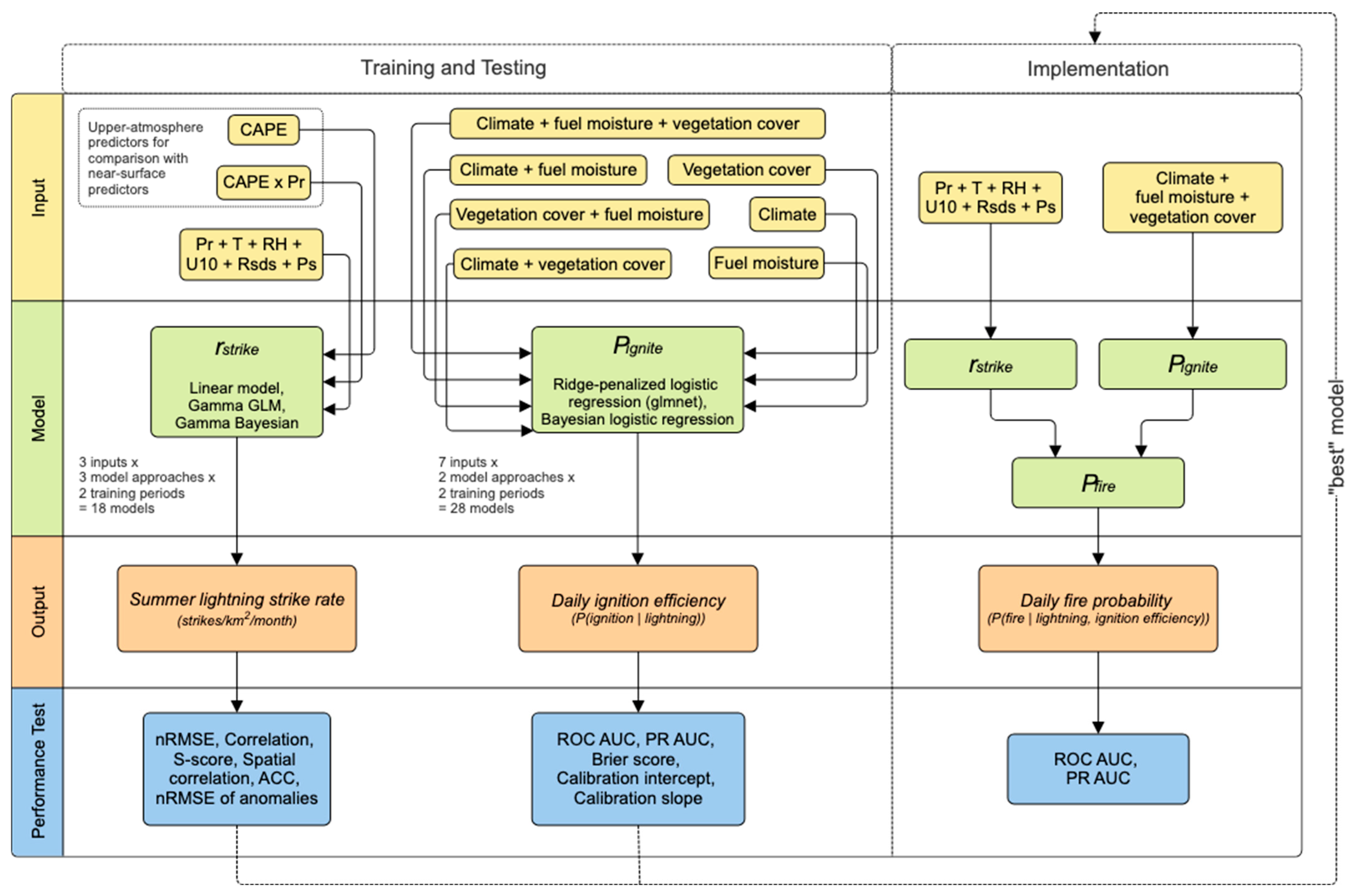
Lightning-caused fire occurrence was modeled as a two-step process in which (1) the rate of lightning strikes and (2) the probability that an individual strike ignites a fire are estimated separately and then combined to estimate the overall probability of fire. Figure 2 provides an overview of our workflow. We first trained lightning and ignition models, which varied according to input predictors, modeling approach, and training period (2002–2011 vs. 2012–2018). Models were evaluated across multiple performance metrics. The lightning and ignition models with the best overall balance across metrics were then implemented into the fire probability Bernoulli model. Finally, fire probability predictions from this working model were evaluated against fire observations.
Lightning and fire occurrence are rare events, making observational datasets highly zero-inflated. Excessive zero values can dominate model fitting, reduce a model’s ability to detect relationships between event and predictors, and bias parameters toward predicting no occurrence. To reduce the number of zero outcomes and focus the analysis on periods when lightning and fire activity are most likely, we limit the training data to the summer fire season, June–August. This practice has been applied to other lightning prediction and fire ignition models [12,23,29,47].

2.2.1. Lightning Strike Rate, rstrike

To predict the spatial and temporal distribution of lightning activity, we retrained a model developed by Uden et al. [30] that relates near-surface climate variables to cloud-to-ground lightning strike rates. We deliberately use near-surface climate predictors rather than upper-atmospheric data, as they are widely available in paleoclimate reconstructions, and have demonstrated comparable performance. These models were re-parameterized for Alaska using the climate and lightning data described above. For each summer season (June–August) and gridcell, we calculated the mean lightning strike rate (strikes/km2/month) and associated averages of temperature, precipitation, wind, relative humidity, shortwave radiation, and surface pressure. The data were split into train (80%) and test (20%) sets and predictor variables were z-score standardized.
Seasonal lightning activity was modeled as a climate-dependent random variable representing the expected rate of lightning strikes per unit area. Let y i = r s t r i k e denote the observed summer-season lightning strike rate in gridcell i and let x i be a vector of standardized near-surface climate predictors. We tested three statistical approaches to predicting r s t r i k e : a linear model, a Gamma generalized linear model (GLM), and a Gamma Bayesian model.
Linear Model
In the linear formulation, lightning strike rate was assumed to follow a Gaussian distribution:
y i | μ i ,   σ ~ N o r m a l ( μ i , σ 2 ) , μ i = a + x i b ,
where a is an intercept, b is a vector of regression coefficients, and σ is the residual standard deviation. This model was fitted using the base R lm() function [48].
Gamma GLM
To account for the strictly positive and right-skewed nature of lightning strike rates, we also fit a Gamma GLM with a log link:
y i |   μ i , κ     ~   G a m m a ( k ,   k / μ i ) , l o g ( μ i ) = a + x i b ,
where k is a shape parameter controlling dispersion and μ i is the expected strike rate. a and b were fitted in base R using glm() with family = Gamma(link = log) [48].
Gamma Bayesian
Finally, we fit a Bayesian Gamma model where both the shape and rate parameters of the Gamma distribution were allowed to vary as functions of climate:
y i |   α i , β i   ~   G a m m a ( α i , β i ) , l o g ( α i ) = a α + x i b α , l o g ( β i ) = a β + x i b β .
All regression coefficients were assigned Normal priors,
a α , a β ,   b α ,   b β   ~   N o r m a l ( 0 , 1 ) ,
and posterior inference was performed using four Hamiltonian Monte Carlo chains in the rstan package version 2.21.8 [49] in R. This formulation allows both the mean and variance of lightning strike rates to respond to climate variability.

2.2.2. Lightning Ignition Efficiency, Pignite

We model ignition efficiency using climate (precipitation, temperature, relative humidity, wind), fuel moisture variables (fine fuel moisture code, duff moisture code, and drought code), and vegetation cover (conifer, broadleaf, and unvegetated/open land). Following methods from Hessilt et al. [12], spatial buffers were applied to each fire to select lightning strikes within 2.5 km or 500 m (depending on the earlier or later dataset, respectively). We then filtered strikes that occurred within 1 day after (to account for inaccuracies in fire detection) and 120 h before the fire. One hundred and twenty hours represents the point at which true lightning-caused ignitions can no longer be reliably distinguished from chance co-occurring lightning strikes (according to methods from Hessilt et al. [12]), rather than the true upper bound on holdover fires, which can extend far beyond this period [4,5]. When multiple strikes fell within the spatial and temporal buffer of a fire, proximity index A was calculated (derived from distance to and time since the fire) to select the best match [50]. This resulted in 278 and 32 fire-causing strikes for the 2002–2011 and 2012–2018 training periods, respectively.
Fire-causing lightning strikes were assigned a value of 1. Non-fire-causing strikes were sampled without replacement from the same temporal windows as the fire-causing strikes, but not spatially near to fire ignitions. Non-fire-causing strikes were assigned a value of 0. This approach preserves the temporal structure of lightning activity and fire weather conditions while preventing spatial autocorrelation between 1 and 0 outcomes.
To mitigate zero inflation, we sample ten non-fire-causing strikes for every fire-causing strike. This strategy improves model generalization by providing sufficient contrast between ignition and non-ignition cases while avoiding the strong class imbalance characteristics of the raw lightning dataset. We also tested a ratio of five 0 outcomes to each 1 outcome and compared sampling methods using model fit (Appendix A). While the 1:5 sampling ratio provided small improvements to class discrimination, models trained on the larger dataset (sampling ratio of 1:10) were consistently better calibrated.
Each lightning strike was associated with climate, fuel, and land cover data (Figure 1c–l) based on date and proximity to the nearest ERA5 gridcell. The data were split into train (80%) and test (20%) sets and predictor variables were z-score standardized. We tested the performance of all combinations of climate, fuel moisture, and landcover predictors (i.e., additive effects of just one predictor grouping, as well as combining predictor groupings) and compared performance between the two training periods (2002–2011 and 2012–2018).
Ignition efficiency was modeled as the probability that an individual lightning strike results in a wildfire ignition. Let z j { 0 , 1 } indicate whether lightning strike j ignited a fire and x j denote a vector of standardized daily predictors, including near-surface climate, fuel moisture indices, and vegetation cover. Ignition outcomes were modeled using logistic regression with a Bernoulli likelihood:
z j | p j   ~   B e r n o u l l i ( p j ) ,   l o g i t ( p j ) = η j = β 0 + x j β , p j = P i g n i t e ,     j = 1 1 + e x p ( η j ) ,
where p j = P i g n i t e is the probability of ignition for strike j. We used two approaches to fit β 0 and β : a ridge-penalized logistic regression (also applied by Hessilt et al. [12]) and a Bayesian logistic regression.
Ridge-Penalized Logistic Regression
Hessilt et al. [12] use a ridge-penalized logistic regression to account for correlation between predictor variables (see Appendix C.2), which often leads to unstable logistic regression. This approach also handles extreme class imbalance and focuses on predictive performance rather than variable selection. Here, we apply the same model. β 0 and β are estimated by minimizing the ridge-penalized loss function, l r i d g e :
l r i d g e ( β 0 , β ) =   j = 1 n [ z j l o g ( p j ) + ( 1 z j )   l o g ( 1 p j ) ] + λ κ = 1 κ β κ 2 .
λ   0 is the ridge penalty parameter, and κ is the number of predictors. The intercept β 0 is not penalized. The coefficient estimates are found as
β ~ N o r m a l ( 0 , τ 2 ) λ = 1 2 τ 2 ,
where τ is the prior standard deviation of each β κ . This model was fitted using the glmnet package version 4.1.9 in R with 5-fold cross validation [51].
Bayesian Logistic Regression
The Bayesian logistic regression replaces the penalty with explicit priors centered at zero for both β 0 and β , and estimates the full posterior distribution of these parameters:
β 0   ~   N o r m a l ( 0 ,   σ β 0 2 ) , β ~   N o r m a l ( 0 ,   σ β 2 ) ,
with posterior distribution
p ( β 0 ,   β | z ) j = 1 n B e r n o u l l i ( p j ) p ( β 0 ) p ( β ) ,
where
p j = l o g i t 1 ( β 0 + x j β ) .
Posterior inference was performed using four Hamiltonian Monte Carlo chains in R’s rstan package version 2.21.8 [49].

2.2.3. Fire Probability, Pfire

After selecting the best r s t r i k e and P i g n i t e models using performance metrics described in Section 2.3 and Table 1, we combine these components to estimate the total probability of lightning-initiated fire, Pfire. Because our strike rate model outputs an expected rate, we do not simulate integer strike counts. Instead, let r s t r i k e , m be the modeled monthly strike rate (strikes/km2/month for June, July, and August) and D m be the number of days in that month m. We convert this to a daily strike rate:
r s t r i k e , d = r s t r i k e , m D m
The probability of at least one ignition in a given gridcell day, I d , is
P f i r e , d = P ( I d 1 ) = 1 ( 1 P i g n i t e , d ) r s t r i k e , d
As the probability of a positive outcome (a single strike results in fire ignition; P i g n i t e , d ) increases and the number of independent events (rate of lightning strikes; r s t r i k e , d ) increase, then so does the overall probability of a positive outcome (at least one strike ignites a fire; P f i r e , d ). Alternatively, when climate conditions are conducive to a high P i g n i t e , but low r s t r i k e (or vice versa), the overall probability of a fire ignition remains low.
Although the Bernoulli model usually assumes discrete trials, using a continuous rate ( r s t r i k e , d ) as the exponent is equivalent to a Poisson-derived formulation under rare-event approximation: 1 e x p ( r s t r i k e , d · P i g n i t e , d ) [52]. This approximation holds when the expected number of ignition events per gridcell-day (the product of strike rate and ignition probability) is very small. Given the observed fire prevalence of ≈1.55 × 10⁻⁵ (fire days divided by total days) during 2002–2011, this condition is satisfied.

2.2.4. Random Forest Models

Prior to model fitting, we used random forest models to assess the relative importance of candidate predictor variables to both lightning strike rate and ignition efficiency. Random forests evaluate variable importance by measuring the increase in prediction error when predictor values are permuted (%IncMSE), and the reduction in node impurity attributed to splits on each variable (IncNodePurity). These analyses were conducted in R using the random Forest package version 4.7.1.1 [53] and are described in more detail in Appendix C. Results informed predictor selection and are reported alongside model comparisons in Section 3.

2.3. Performance Metrics

Given that the target outcome differs for each model, we apply different performance metrics for r s t r i k e , P i g n i t e , and P f i r e . Metrics include for r s t r i k e : normalized RMSE (nRMSE), Pearson correlation, S-score [54], spatial correlation, anomaly correlation coefficient (ACC), and nRMSE of anomalies; for P i g n i t e : area under the receiver operating characteristic curve (ROC AUC), area under the precision-recall curve (PR AUC), Brier score, and calibration regression intercept and slope; and for P f i r e : ROC AUC and PR AUC. We also tested the model’s ability to reproduce observed fire counts by comparing ∑ P f i r e with the total number of observed fires in the simulation period. Appendix B provides in-depth descriptions of these metrics. For brief metric descriptions and interpretations, refer to Table 1.
The two training periods differ substantially in both sample size (2002–2011: n = 1112, 2012–2018, n = 128) and lightning detection accuracy, which introduce a trade-off between data quantity and quality. To quantify the uncertainty associated with each model’s performance, we calculated 95% bootstrap confidence intervals for all evaluation metrics. For each model, we generated 1000 bootstrap samples by resampling the test dataset with replacement, each sample having the same size as the original test set (20%). Performance metrics were recalculated for all bootstrap samples and confidence intervals were obtained using the 2.5th and 97.5th percentiles of the resulting bootstrap distribution. This approach provides a non-parametric estimate of uncertainty that reflects differences in sample size and data accuracy across training periods.
Performance metrics for r s t r i k e and P i g n i t e were calculated from test data. To calculate metrics for Pfire, observations of fire point locations were converted to binary events, so that each day and gridcell (0.25° × 0.25°, matching the resolution of the training data) contains either a 1 (at least one lightning-caused fire occurred) or 0 (no lightning-caused fire occurred). This allows predicted probabilities to be compared with binary observations.
We also tested out-of-period performance of r s t r i k e and P i g n i t e models selected for implementation into the P f i r e model based on in-period performance by applying parameters estimated from one period to the alternate period (i.e., 2002–2011 parameters → 2012–2018 data and 2012–2018 parameters → 2002–2011 data).

2.4. Use of Artificial Intelligence

OpenAI’s ChatGPT (GPT-4o; March 2026) was used during development of R and Python code. All code and data output was reviewed for quality and accuracy. We take full responsibility for the content of this manuscript.

3. Results

3.1. Lightning Strike Rate, rstrike

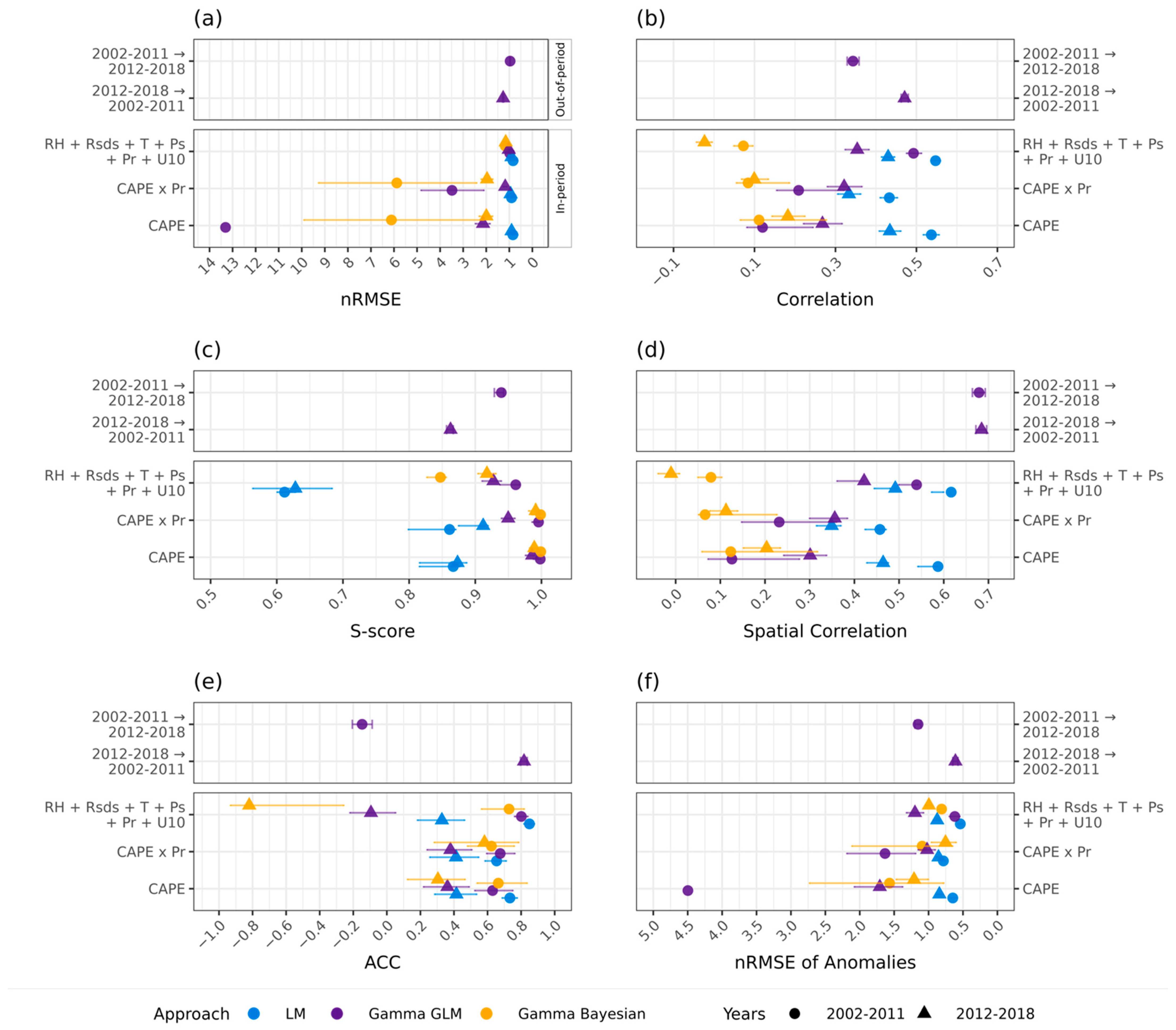
We applied a random forest [53] to understand the relative importance of each near-surface climate variable in predicting lightning strike rate for the 2002–2011 and 2012–2018 periods (Appendix C.1). Some variables, particularly relative humidity, consistently rank high in importance, although the relative importance of individual variables differed somewhat between metrics and time periods. Because all variables contributed some predictive value, we chose to include all six as predictors for our lightning prediction models. Using the six metrics described in Table 1, we compare model families (Linear, Gamma GLMs, and Gamma Bayesian), predictors (CAPE-based vs. near-surface), and training period (2002–2011 vs. 2012–2018) in Figure 3.

3.1.1. Modeling Approach and Predictor Groups

Linear models exhibited low nRMSE (0.84–0.94), moderate correlation (0.33–0.55), relatively strong spatial correlation (0.35–0.62) and successfully captured interannual variability during the longer training period (ACC = 0.61–0.79; nRMSE of anomalies = 0.54–0.79). However, these models predict occasional negative strike rates, which are physically unrealistic, and were, therefore, excluded from subsequent fire calculations.
Gamma GLMs showed the best overall balance among models that enforce non-negative strike rates. For CAPE-based predictors, Gamma GLMs performed poorly across most metrics (nRMSE = 2.14–13.31; correlation = 0.12–0.32; spatial correlation = 0.13–0.36; nRMSE of anomalies = 1.02–4.50) but achieved high S-scores (S-scores = 0.99), indicating that they reproduce the marginal distribution of lightning despite failing to capture its magnitude, spatial pattern, or interannual variability. In contrast, near-surface Gamma GLMs showed substantially improved fit across metrics (nRMSE = 0.98–1.02; correlation = 0.35–0.49; spatial correlation = 0.42–0.54; nRMSE of anomalies = 0.54–1.20) but had lower S-scores (0.61–0.96). This suggests that the model captures the geographic pattern and distributional shape of lightning reasonably well (spatial correlation and S-score), but not the precise magnitude (correlation).
Bayesian Gamma models did not consistently outperform the Gamma GLMs. These models degraded correlation (−0.02–0.19) and spatial correlation (−0.01–0.22) and showed mixed anomaly performance (ACC = −0.82–0.80; nRMSE of anomalies = 0.56–1.88), though they captured the observed frequency distribution well (S-score = 0.95–0.99).

3.1.2. Training Period

A comparison between training periods demonstrates that models trained on the longer 2002–2011 period (circles, Figure 3) generally outperformed those fit to 2012–2018 (triangles, Figure 3), despite lower lightning detection accuracy prior to 2012. For example, the near-surface Gamma GLM achieved higher correlation (0.49 vs. 0.35), higher spatial correlation (0.54 vs. 0.42), and better anomaly magnitudes (nRMSE of anomalies = 0.54 vs. 1.20) when trained on the earlier period, while maintaining similar nRMSE (0.98 vs. 1.02). Bootstrapped confidence intervals confirmed that nRMSE differences across periods were not statistically significant, indicating that additional years of climate variability outweighed improvements in detection accuracy for model generalization.

3.1.3. Model Selection

These results demonstrate that near-surface predictors, when used in combination, are a viable substitute for CAPE-based models, consistent with findings from Uden et al. [30]. For the intended paleo application, stronger spatial agreement and interannual anomaly tracking seen in the Gamma GLMs are more relevant, as regime–scale comparisons of relative fire activity are more robust than absolute strike rate estimates at the daily or gridcell level. Based on these findings, we selected the near-surface Gamma GLM approach trained on 2002–2011 data as the r s t r i k e component of P f i r e .

3.1.4. Cross-Validation Across Time Periods

To check for temporal transferability of the near-surface Gamma GLM (selected for application in P f i r e ), we applied parameters estimated from each period to data from the alternate period and compared their performance (Figure 3a–f, top facets) with in-period predictions (Figure 3a–f, bottom facets). The 2002–2011 parameters applied to 2012–2018 data perform comparably or better than the 2012–2018 in-period predictions according to most metrics (nRMSE: from 1.02 to 0.96; spatial correlation: from 0.42 to 0.68; S-score: from 0.93 to 0.94). ACC shows the most notable degradation (worsening from −0.1 to −0.15), indicating a decline in the model’s ability to track year-to-year changes in lightning (though the magnitude of anomalies is better captured according to nRMSE of anomalies).
The 2012–2018 parameters applied to 2002–2011 data show improvements to spatial correlation, ACC, and nRMSE of anomalies, though nRMSE (from 0.98 to 1.27) and S-score (from 0.96 to 0.86) degradation indicate the 2012–2018 parameters are less robust when applied outside their training period. Given these results, while neither near-surface Gamma GLM shows perfect out-of-period performance, the forward cross-period transfer confirms that the 2002–2011 parameters generalize well to new data, supporting their selection for paleo applications.

3.2. Ignition Efficiency, Pignite

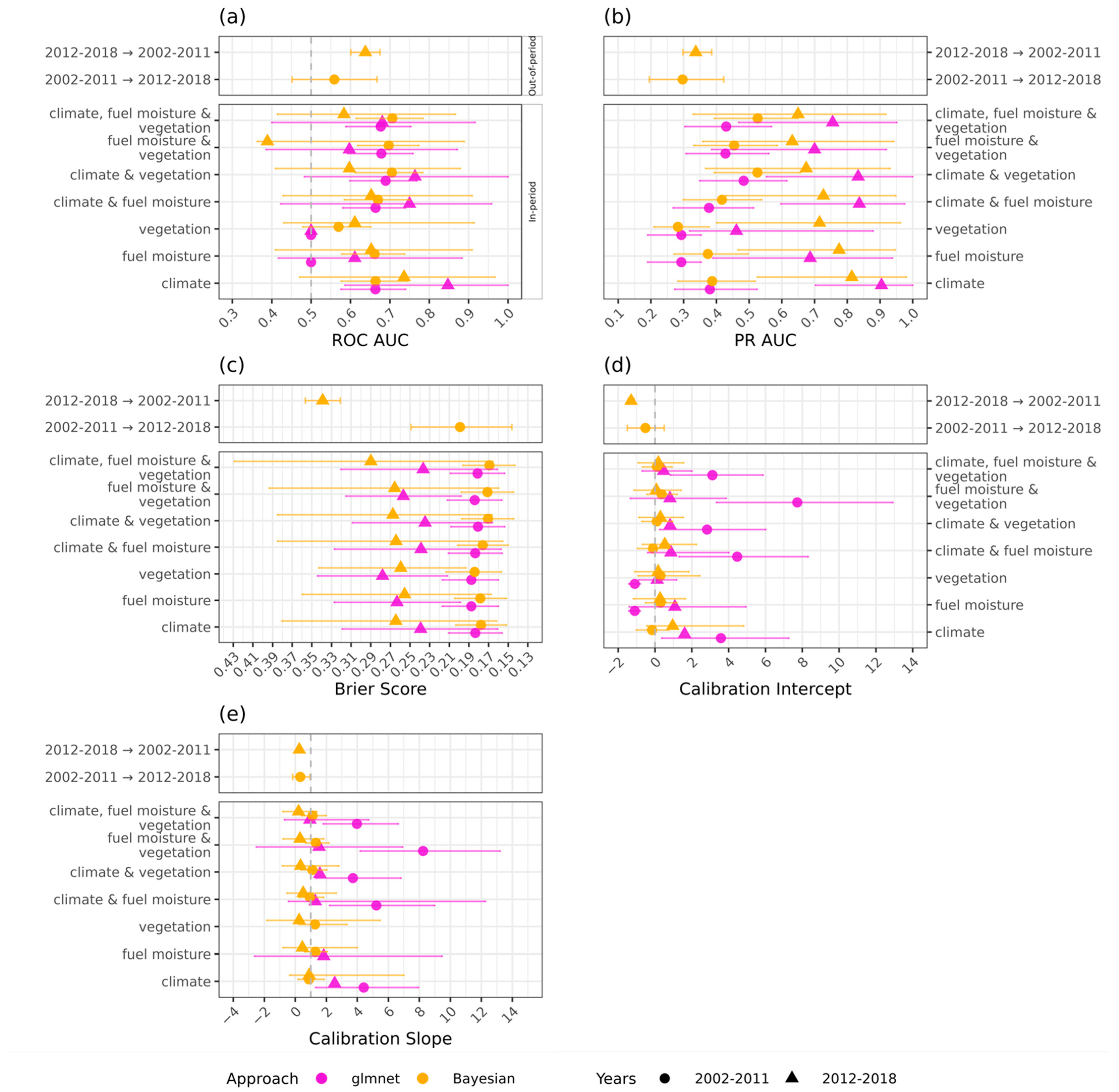
We again applied a random forest to assess variable importance, this time in predicting ignition efficiency (Appendix C.2). Fuel moisture indices, temperature, relative humidity, and precipitation hold the greatest importance, while wind and vegetation show less contribution to ignition prediction. Overall, the earlier 2002–2011 period displayed better importance values than the 2012–2018 period. We then evaluated two modeling approaches to predicting lightning ignition efficiency (glmnet ridge regression vs. a Bayesian logistic model), seven predictor groupings (climate, fuel moisture, vegetation, and their combinations), and two training periods (2002–2011 vs. 2012–2018). Model performance was assessed using five metrics described in Table 1 and compared in Figure 4.
The event prevalence is used as a point of comparison for PR AUC, representing a model with no skill in ranking ignition probability (Figure 4b). Because lightning-caused fires are extremely rare events, the baseline event prevalence before subsampling zero-outcome lightning strikes (lightning-caused fire count/total lightning count) is very low, corresponding to 1.55 × 10⁻⁴ for 2002–2011 and 1.89 × 10⁻⁵ for 2012–2018. When interpreting PR AUC, absolute values are not directly comparable to real-world prevalence. Instead, relative comparisons across models are used to assess performance.

3.2.1. Predictor Groups

Models which used only a single-predictor group (i.e., just climate, fuel indices, or land cover) showed clear differences in skill. Climate-only models performed best among single group predictors (ROC AUC = 0.66–0.85). Vegetation-only models performed worst (ROC AUC = 0.50–0.61; PR AUC = 0.28–0.72; Brier = 0.18–0.28), although all models substantially exceed the PR AUC no-skill baseline given the rarity of ignition events. Fuel moisture-only models performed moderately well (ROC AUC = 0.61–0.66), indicating some ability to rank ignition risk. However, for the glmnet fuel-only and vegetation-only models, calibration slopes could not be estimated (Figure 4e). This occurred because ridge penalization shrank all regression coefficients toward zero, yielding nearly constant predicted ignition probabilities (ROC AUC = 0.5; no skill). With all model predictions collapsing to similar values, there is no variation in predicted probabilities against which to assess whether the model is well-scaled, confirming that these models have no meaningful discriminative skill. Combining predictor groups improved performance: models using climate + vegetation or all predictors consistently produced higher discrimination (ROC AUC = 0.67–0.71 for 2002–2011 and 0.58–0.76 for 2012–2018) and lower Brier scores (=0.17–0.24), indicating that ignition efficiency depends on both climate and fuel related conditions.

3.2.2. Modeling Approach

Model families differed in calibration. Bayesian models exhibited the best-calibrated probability estimates during 2002–2011, with calibration intercepts near zero (−0.16–+0.36; 0 = no bias) and calibration slopes close to one (0.88–1.33; 1 = perfect calibration), indicating that predicted probabilities were neither systematically too high nor too low, and scaled proportionally to observed ignition rates. That is, ignition probabilities produced by the Bayesian models are well-scaled to observed fire. In contrast, glmnet models showed slopes farther from ideal (3.7–8.2) and larger intercepts (2.8–7.7) during the same period, consistent with overconfident predictions. The 2012–2018 glmnet models achieved high discrimination (ROC AUC = 0.60–0.85; PR AUC = 0.70–0.90) but displayed highly unstable calibration parameters with extremely wide bootstrap confidence intervals, reflecting small sample sizes and class imbalance. Bayesian models during 2012–2018 were more stable but showed reduced discrimination relative to the earlier period (ROC AUC = 0.39–0.74; PR AUC = 0.63–0.81).

3.2.3. Training Period

Training on the longer 2002–2011 period consistently produced ignition probabilities that more closely reflect observed ignition rates and reduced uncertainty across both model families. The shorter 2012–2018 period, despite improved lightning detection accuracy, amplified data scarcity and class imbalance, producing higher discrimination for glmnet but at the cost of unstable calibration and wider confidence intervals. In fact, for several glmnet models trained on the 2012–2018 period (e.g., climate-only and climate + vegetation), bootstrap confidence intervals for calibration slope and intercept were extremely wide (upper limits > 100), reflecting quasi-complete separation in some bootstrap resamples rather than meaningful parameter values. This indicates that, under the limited sample size and strong class imbalance of the later period, small changes in the data lead to large changes in the calibration fit, and the resulting probabilities are not numerically stable. Statistical stability in these ignition models benefits more from sample size and climate variability than from improvements in lightning detection accuracy alone.

3.2.4. Model Selection

Model choice depends on whether ignition probabilities are used for ranking or for physical interpretation. If well-calibrated ignition probabilities are required for downstream modeling (e.g., fire probability), Bayesian models trained on 2002–2011 offer the best balance of discrimination, calibration (among in-period predictions), and stability. If only relative risk ranking is needed, glmnet models from 2012–2018 achieve the highest ROC AUC values but produce unreliable probability estimates. Vegetation-only and fuel + vegetation models show limited discriminative power (results that are consistent with Hessilt et al. [12]).
However, vegetation in combination with climate and fuel does not degrade model performance and may allow spatial transferability across ecoregions. We therefore chose to retain vegetation predictors, prioritizing generalizability over maximum parsimony. Given these results, we selected the Bayesian logistic regression trained on climate, fuel moisture, and vegetation cover from the 2002–2011 period.

3.2.5. Cross-Validation Across Time Periods

We again check the transferability of parameter estimates by applying models from each period to data from the alternate period (top vs. bottom facets of Figure 4a–e), comparing the earlier and later Bayesian logistic regression trained on climate, fuel moisture, and vegetation cover. Neither model transfers perfectly: both out-of-period calibration slopes (0.33 and 0.26) are far from ideal (1), indicating overconfident predictions in both cases. A key difference is in Brier score: the 2002–2011 parameters applied to 2012–2018 data produce a Brier score of 0.20, which is an improvement over the 2012–2018 in-period Brier score of 0.29. The reverse transfer substantially worsens Brier score (2012–2018 out-of-period: 0.34 vs. in-period: 0.17; lower values indicate better prediction accuracy).
ROC AUC shows a different pattern. The 2002–2011 out-of-period predictions produce lower ROC AUC values than the in-period model, with wide confidence intervals reflecting the limited sample size of the 2012–2018 data (consistent with findings in Section 3.2.3). For the intended paleo application, we chose to prioritize accurate probability estimates (Brier score) over discrimination ranking (ROC AUC). With this in mind, we maintained our selection of the 2002–2011 parameter estimates for application in P f i r e .

3.3. Fire Probability, Pfire

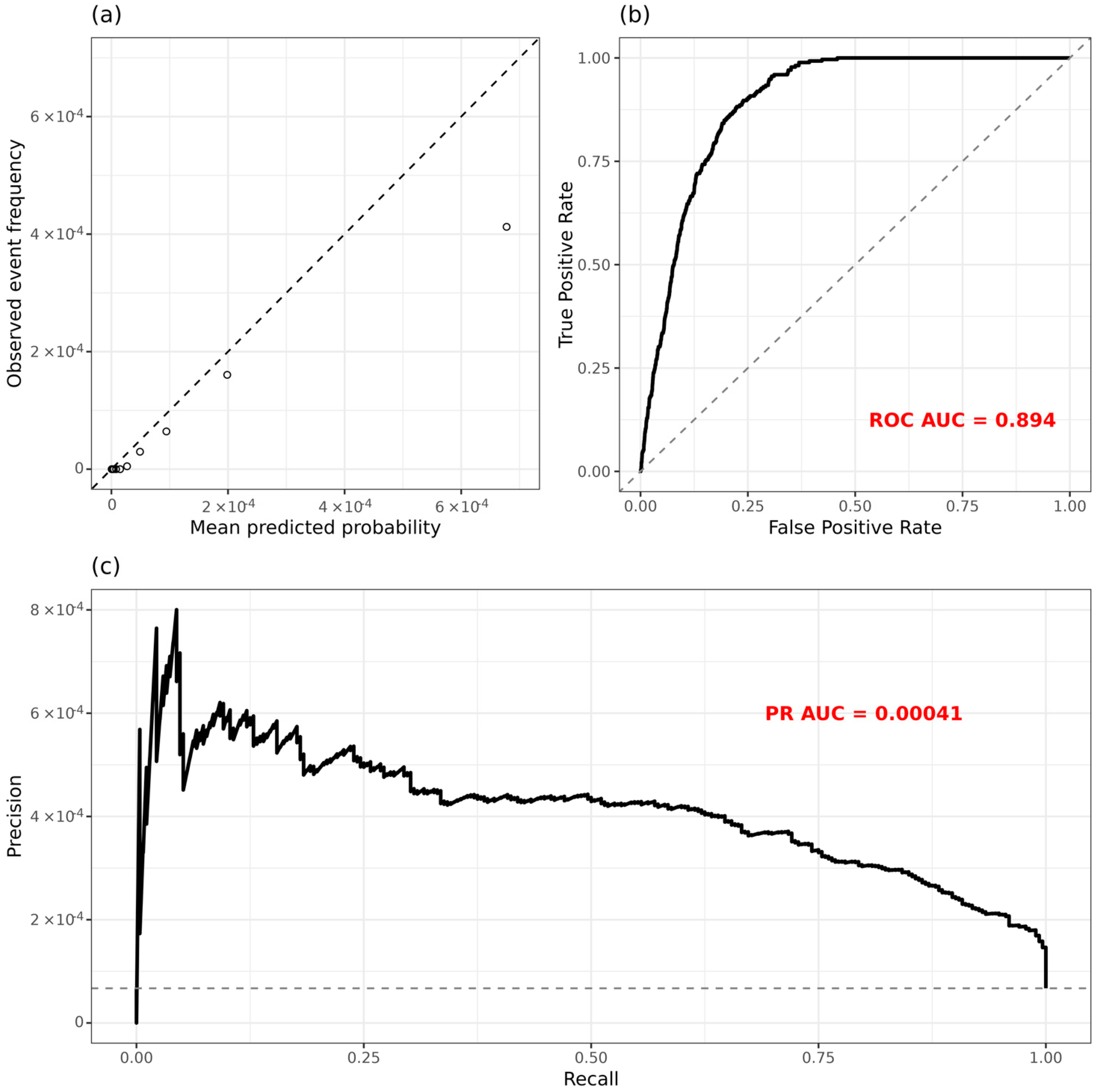
Based on results from Section 3.1 and Section 3.2, P f i r e was estimated using the Gamma GLM lightning model and Bayesian ignition efficiency model, both trained on the 2002–2011 period using all predictors. Figure 5a compares predicted probabilities with observed frequencies of lightning-caused fire using quantile-based bins. At very low probabilities, predicted and observed frequencies fall slightly below the 1:1 line, indicating that the model is calibrated to the background risk regime with slight overprediction. As predicted probabilities increase, however, overestimation of the likelihood of fire progressively increases. In the highest probability bin, predicted probabilities sum to ~262 fires, but only 164 fires are observed. This indicates that the model captures the relative ranking of fire risk (good discrimination) but inflates probabilities in high-risk conditions (imperfect calibration).
The ROC curve (Figure 5b) indicates strong discrimination skill (ROC AUC = 0.894, with ROC AUC = 1 indicating a perfect model); days with lightning-caused fires are consistently assigned higher probabilities than non-fire days. Because lightning-caused fires are rare events (272 fires across ~4 million gridcell-days), the baseline PR AUC (Figure 5c, dashed horizontal line) equals the event prevalence (≈0.000067). The model achieved a PR AUC of 0.00041, approximately 2.6 times higher than the baseline rate, indicating improvement over random classification. Furthermore, the PR line (solid line) lies above the baseline prevalence rate (dashed horizontal line), demonstrating that high-probability predictions occur when observed fires occur. Together, these results indicate that the model effectively ranks fire risk (when and where fire risk is elevated), though it overestimates the magnitude of this risk.
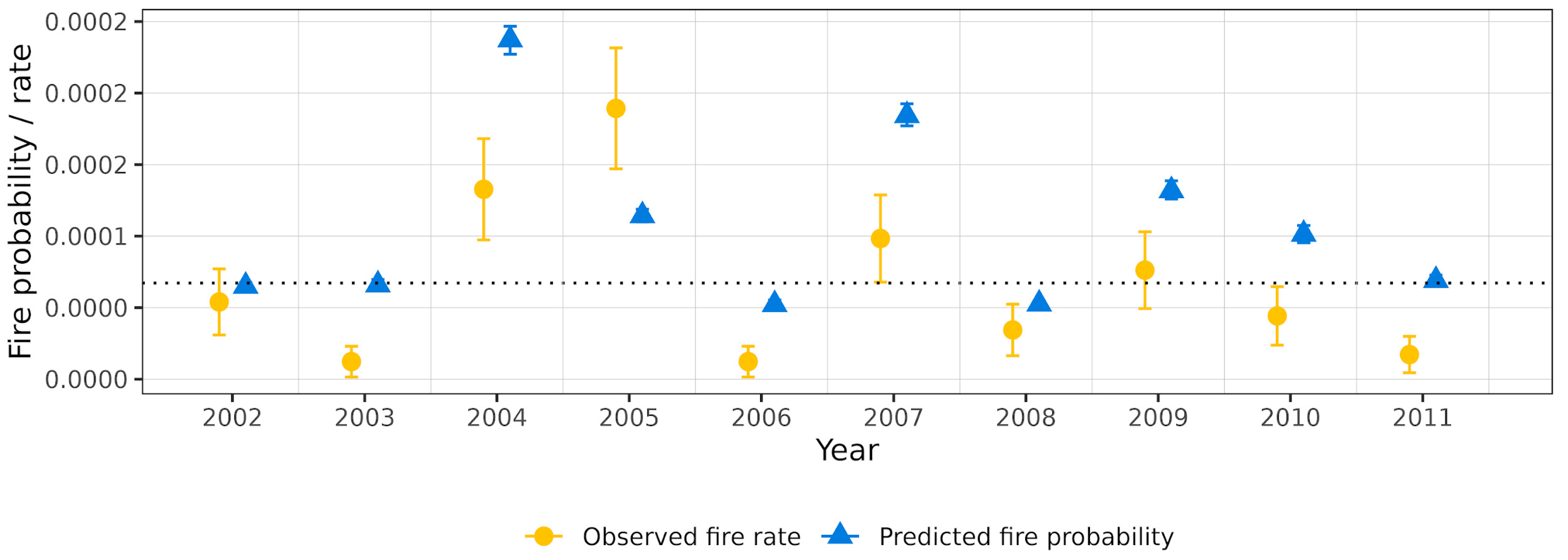
These results are reflected in Figure 6, which compares deviations of annual observations (yellow) and predictions (blue) from the 10-year climatology (dotted horizontal line). Across most years, model predictions correctly track the direction of observed deviations from the mean. However, the model fails to capture the magnitude of anomalies.
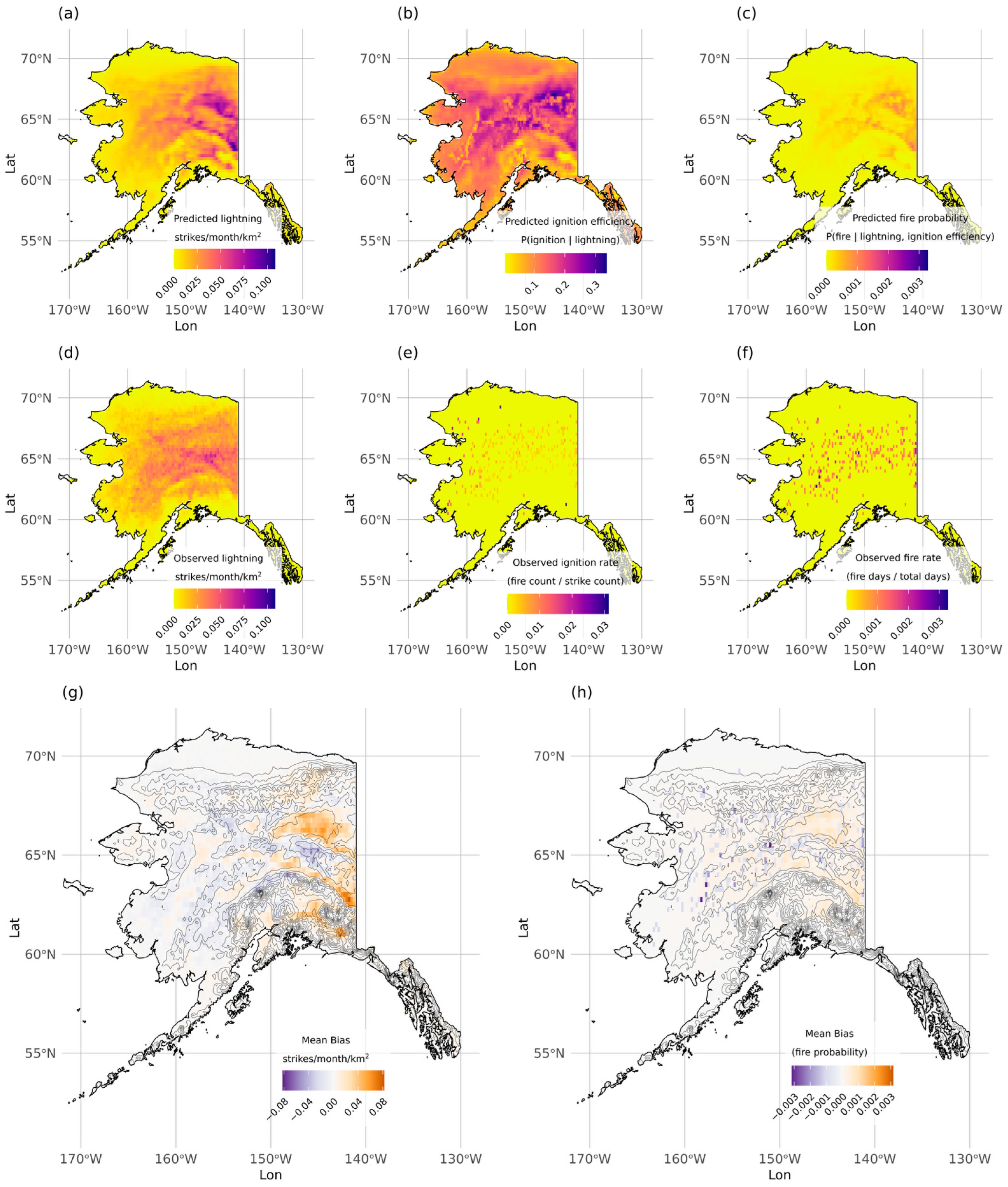
Figure 7 provides a spatial comparison of predictions and observations by mapping strike rates, lightning ignition efficiency, and fire occurrence, as well as lightning and fire probability prediction bias. Predicted lightning strike rates (Figure 7a) correspond well to observations (Figure 7d), with coastal areas experiencing strike rates close to 0 strikes/month/km2 and rates increasing towards the interior of Alaska. However, the lightning model over-estimates strike rates in certain regions, for example assigning average values of up to 0.1 strikes/month/km2 in east-central Alaska, where only 0.05–0.075 strikes/month/km2 were observed (Figure 7a,d). Figure 7g shows the spatial distribution of lightning prediction bias. Bias appears greatest in Eastern interior Alaska. Overprediction (orange gridcells) occurs in low-lying relatively flat regions, though the higher-elevation Copper River Basin in southern Alaska also sees overprediction. Bias switches from over to underprediction (purple gridcells) where elevation starts to increase. Low bias occurs in coastal regions where observed lightning is infrequent.
The spatial distribution of ignition efficiency predictions is compared with observations by dividing lightning-caused fire counts by total lightning counts for each gridcell. Though predicted probabilities of lightning-caused ignitions differ from observations by one order of magnitude, this is due to the large class imbalance in the raw data, which contains 1,882,857 lightning strikes and just 278 fires. To mitigate zero inflation, we subsample 0-outcome strikes, allowing the model to successfully separate ignitions from non-ignitions. In Figure 7b, predictions capture the relative spatial distribution of observations seen in Figure 7e but overestimate absolute values. A per-gridcell bias metric is not computed for ignition efficiency because the observed ignition rate (fires/strikes) is not directly comparable to the model’s ignition efficiency estimates.
Despite this, mean fire probability predictions (Figure 7c) correspond well to observed rates (Figure 7f; calculated for each gridcell as the number of fire days/total days), with areas of high predicted fire risk occurring where fires were more frequently observed. Figure 7h displays locations of under (purple gridcells) and overprediction (orange gridcells) of fire probability. A comparison with elevation indicates that overprediction occurs in flat, low-lying regions of Eastern interior Alaska, while underprediction occurs in flatter regions of Western interior Alaska. Spatial patterns in fire probability bias correspond to those of the lightning model.

4. Discussion

This study aimed to develop a lightning-caused fire framework that (1) decomposes fire occurrence into lightning frequency and ignition efficiency and (2) relies exclusively on predictor variables available in paleoclimate reconstructions. Our results demonstrate that both objectives were achieved. Near-surface climate predictors reproduced spatial and temporal variability in lightning strike rates with comparable skill to CAPE-based models, and Bayesian ignition models provided well-calibrated ignition probabilities. When combined in a Bernoulli framework, these components effectively ranked fire risk across Alaska while preserving physical interpretability. All predictor variables used here (near-surface climate, fuel moisture indices, and vegetation cover) are available in paleo datasets, making these methods transferable into the past.

4.1. Process Separation and Interpretability

A key contribution of our methods is the explicit separation of lightning occurrence and ignition efficiency, which preserves interpretability by allowing for climate sensitivities to differ across processes. Figure 7 illustrates this spatially: regions of high ignition efficiency in northern Alaska do not translate to high fire probability due to low strike rates, while the interior, where high strike rates and ignition efficiencies coincide, has higher predictions of fire probability. This compound structure constrains unrealistic fire occurrence in regions lacking ignition sources. With the exception of Hessilt et al. [12], current lightning–fire parameterizations do not make this separation [11,31,32,33].
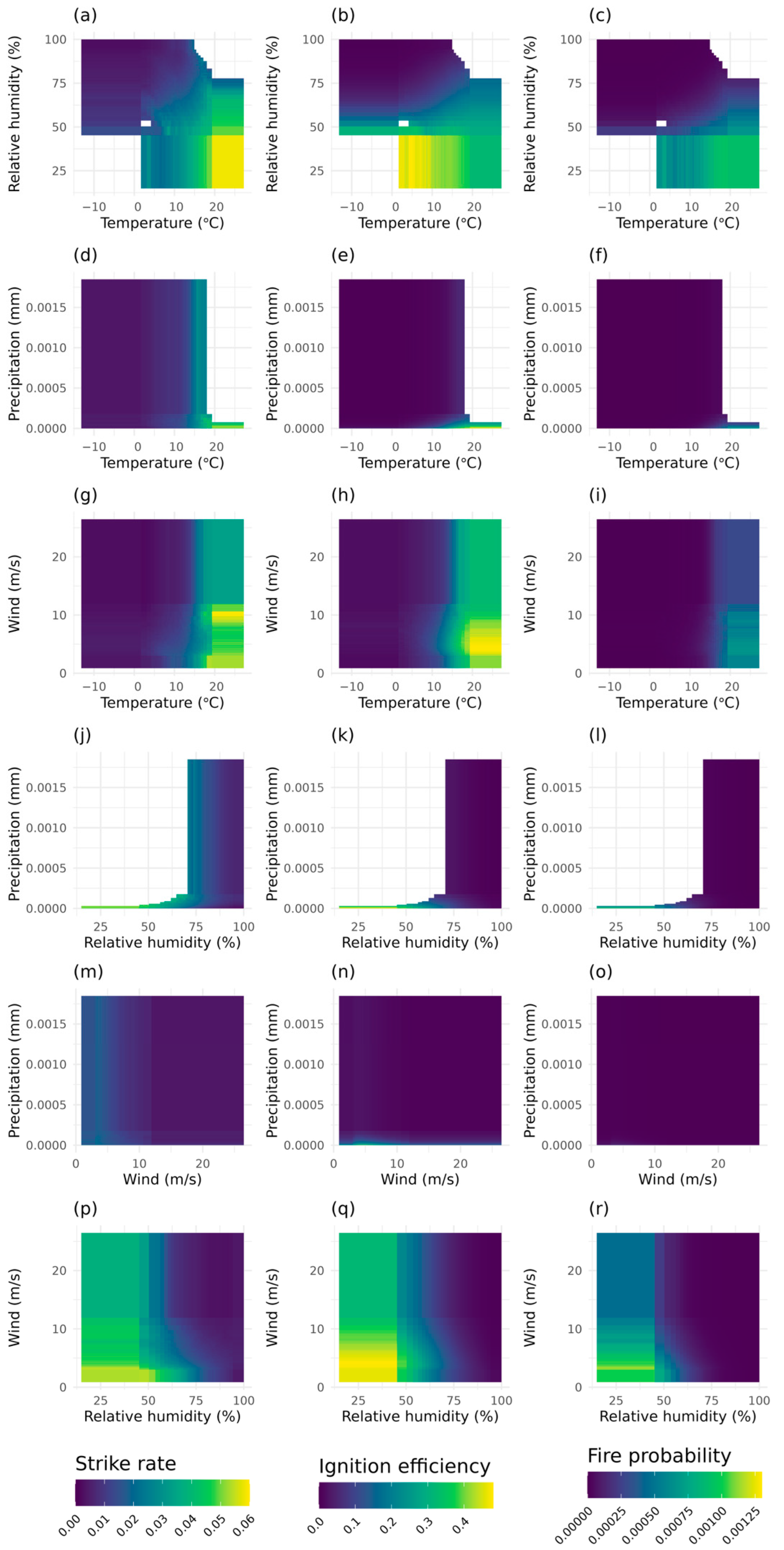
Figure 8 further demonstrates the interpretive value of this separation by displaying the conditional effects of temperature, relative humidity, precipitation, and wind (selected because they serve as predictors in both the lightning and ignition efficiency models) on each model component and their combined fire probability. Across all panels, fire probability (right column) peaks only where lightning (left column) and ignition efficiency (center column) are concurrently high. Temperature acts as a compound predictor: both lightning occurrence and ignition efficiency increase with warming above 10–15 °C, reflecting the role of temperature in driving convective instability and fuel drying simultaneously (Figure 8a–i). Relative humidity reveals a more complex relationship. Ignition efficiency requires the combined effects of low humidity and wind (Figure 8q), whereas lightning activity tends to occur under low humidity and warm temperatures (Figure 8a). Precipitation suppresses ignition efficiency across all variable combinations (Figure 8e,k,n), while lightning is less constrained by precipitation, requiring warm and relatively dry conditions. Wind-precipitation interactions show weak gradients across all three response variables (Figure 8m–o), suggesting limited discriminative power in isolation; the influence of these variables on fire probability is largely contingent on temperature and humidity conditions already favorable for lightning ignition. This ability to interpret how climate drives each component independently makes our modular framework suitable for integration into larger modeling systems.

4.2. Overprediction and Calibration

Overprediction in the highest-risk bins (Figure 5a) may arise from several factors, including the nature of our model framework, unresolved fine-scale variability in the training data, and assumptions about human suppression. Even small overestimates in ignition probability or strike rate will propagate in the expression 1 ( 1 P i g n i t e , d ) r s t r i k e , d ; the Bernoulli model inflates fire probability under high-risk conditions. For example, Figure 7g shows that overestimates of lightning (orange gridcells) concentrate in the Yukon Flats, Tanana–Kuskokwim Lowlands, and Copper River Basin [56], likely driving inflated fire probabilities in the same regions, as seen in Figure 7h.
Furthermore, overprediction could result from the coarse resolution of the training data (0.25° grid). Under extreme conditions, ignition can fail at finer scales due to smaller scale variability in weather, fuel conditions, or vegetation structure that is not represented in the model. That is, while ignition predictions might be high, sub-gridcell variability may not necessarily result in an observed ignition.
Finally, because the framework we have developed intentionally excludes anthropogenic fire interactions, fire detection and suppression could reduce realized fire occurrence relative to climate and fuel conditions alone. In other words, the model may approximate a climate-limited ignition regime rather than the observed regime modified by humans. This was proposed by Krause et al. [57], who report overestimates of global lightning-caused fire predictions and suggest that exclusion of suppression was a contributing factor.
However, this mechanism may be limited for Alaska’s interior region. DeWilde and Chapin [8] found that approximately two-thirds of interior Alaska operates under a mostly natural fire regime with minimal suppression activity, and that large lightning-caused fires dominate burned area in these remote regions. Conversely, human-caused fires in this region tend to be smaller and shorter-lived than lightning-caused fires [10], and human influence on fire occurrence is concentrated within approximately 40 km of settlements, corresponding to ~31% of interior Alaska [9]. Since the highest predicted fire probabilities in our model arise in interior Alaska (Figure 7c), exclusion of anthropogenic interactions in our models may contribute to overestimation of fire probability in this ~31% of the region where human influence on fire is strongest (Figure 7h).
In the context of reconstructing paleo fire regimes, consequences to overprediction may vary according to the period of interest. Charcoal records from interior Alaska suggest that the 2002–2011 training period represents a period of high fire activity relative to Holocene reconstructions. Kelly et al. [13] found that recent burning in the Yukon Flats already exceeds upper fire regime limits of the past 10,000 years, and ice core-derived black carbon records analyzed by Sierra-Hernandez et al. [16] show a marked increase in Alaska’s fire severity since the 1980s.
For paleo simulations targeting periods of low fire activity due to, for example, the absence of flammable red spruce during the early Holocene (10,000–6000 cal BP), or the cool wet climate of the Little Ice Age (500 cal BP) [13], predicted fire probabilities will fall in the low-to-moderate range where our model is well calibrated (Figure 5a; points are close to the 1:1 line). In other words, instances of high-risk conditions where overprediction is concentrated will be rare or absent. However, we caution that during periods of high fire activity, such as the mid-Holocene (6000–3000 cal BP) when flammable black spruce expanded, or the warm dry climate of the Medieval Climate Anomaly (1000–500 cal BP) [13], instances of high-risk bins are more likely (Figure 5a; points fall below the 1:1 line). During these periods, when climate conditions approach or exceed the modern training range, the potential for overestimates of fire risk will increase.

4.3. Training Period Selection

Our comparison across training periods reveals a tradeoff between detection accuracy and sample size relevant to paleo applications. Despite the lower detection accuracy of the 2002–2011 training period, models trained on these data achieved comparable performance across most metrics (Figure 3 and Figure 4). Detection errors in the earlier period introduce noise to the outcome variable. However, despite improved detection, the shorter 2012–2018 period provided insufficient climate variability and fire events for stable parameterization, resulting in wide confidence intervals. For paleo applications, where the goal is to extrapolate from climate states outside the modern range, a training period that captures greater climate variability is more robust.

4.4. Predictor Selection

Lightning polarity has been used in past efforts to estimate ignition efficiency, with the assumption that positive strikes, which provide a longer current, have a greater potential for ignition [58]. For example, the Wildland Fire Assessment System (WFAS) is used by the U.S. Forest Service to determine ignition efficiency and includes polarity. However, other ignition efficiency models applied to Alaska [12] and the contiguous United States [3,59] do not find an association with polarity. Given these contradictions, we chose to exclude this variable from our models.
Elevation was not included as a predictor in our models. Prior studies in Alaska have documented relationships between elevation and lightning strike density, specifying that this relationship is the result of elevation’s influence on convective activity [60,61]. Figure 7g displays the relationship between elevation and lightning prediction bias. Interior Alaska shows a clear pattern: at higher elevations, where observed lightning is frequent, the model underpredicts lightning (purple gridcells) whereas in low-lying flat regions, where observed lightning is infrequent, the model overpredicts (orange gridcells).
This pattern becomes less clear towards coastal regions: bias decreases and over vs. underprediction occurs at both low and high elevation. There appear to be different convective mechanisms occurring here, potentially resulting from coastal proximity where shallower cloud tops and weaker updrafts diminish lightning activity [22,62]. Dissing and Verbyla [61] found frequent lightning occurrences in both mountainous terrain and flat river valleys and Peterson et al. [31] saw differences in fire and lightning activity between Eastern and Western Alaska. This suggests that elevation’s influence on lightning is mediated by local convective conditions rather than acting as a direct predictor.
In the context of ignition efficiency, Hessilt et al. [12] found that elevation and other landscape characteristics were outperformed by fire weather predictors according to ROC AUC values and Calef et al. [9] reported that elevation was a minor driver of lightning-caused fire probability. Still, future work could test whether including elevation improves the performance of our models. Fire probability bias shown in Figure 7h corresponds to locations of lightning prediction bias in Figure 7g. Though not surprising given the pipeline structure of our framework, addressing bias in the lightning model will likely diminish errors in fire prediction.

4.5. Model Integration

Postglacial charcoal analyses reveal that vegetation composition has played an important role in wildfire regimes of boreal Alaska [13,15,16,17]. For example, Kelly et al. [13] propose that warm, dry conditions during the Medieval Climate Anomaly (1000–500 cal BP) drove a rise in fire severity in the Yukon Flats region of interior Alaska, promoting recruitment of early successional, less flammable deciduous species. This vegetation feedback likely limited fire frequency despite climatic conditions conducive to elevated ignition probability. In contrast, the expansion of flammable black spruce during the mid-Holocene (6000–3000 cal BP) drove a sustained rise in fire frequency [13]. These contrasting feedbacks demonstrate that vegetation-fire dynamics are inconsistent across time scales and reinforce the value of process-based models.
Dynamic global vegetation models (DGVMs) are designed to simulate these climate-fire-vegetation feedbacks. However, existing DGVM fire modules such as JULES-INFERNO [63,64], SPITFIRE [65], BLAZE [66], CLM fire module [67], and CTEM fire module [68,69], link fire activity to factors like human population density, human propensity to start or suppress fires, and socioeconomic conditions (as well as lightning ignition). While appropriate for modern contexts, including those discussed in Section 4.2, these assumptions limit their application in paleo settings where human–fire interactions are poorly constrained or simply differ. The framework presented here provides a probability-based ignition mechanism that could be incorporated into DGVM fire modules to understand past climate, lightning, wildfire, and vegetation dynamics.

4.6. Limitations

The use of monthly strike rate aggregates, while necessary to reduce zero inflation common in rare-event modeling, introduces a temporal mismatch with daily ignition probabilities. With a single strike rate prediction assigned to all days within a month, within-month lightning activity is not captured, leaving ignition efficiency as the predominant driver of day-to-day variation in fire probability. For the intended paleo application, where climate reconstructions carry greater uncertainty at sub-seasonal timescales, this is an acceptable tradeoff; regime–scale fire dynamics are better constrained at annual or seasonal resolutions than at the daily time scale. In other words, paleo fire reconstructions would focus on seasonal, decadal, or centennial change in fire regimes, rather than daily forecasting. With this in mind, future work could explore retraining these models on seasonal or summer-aggregated predictors to better accommodate paleoclimate datasets with coarser temporal resolution [39]. Nonetheless, our methods provide a pathway forward for reconstructing past lightning-driven fire regimes from paleo data.
As demonstrated in Figure 5a and discussed in Section 4.2, our fire model tends to overestimate absolute fire probability under high-risk conditions. Other modeling approaches have reported a similar issue [12,57,58], suggesting that this limitation is not unique to this study. Nonetheless, absolute fire counts ( P f i r e ), particularly those derived from high-risk conditions, should be interpreted with caution since they will likely exceed true fire counts. However, the strong discriminatory skill of the model (ROC AUC = 0.894) indicates that the relative ranking of fire risk across space and time is preserved. Once again, for paleo applications, where the goal is to reconstruct long-term trends and relative changes to fire, rather than absolute fire counts, this limitation is less consequential. We expect that the overall temporal and spatial pattern of predicted fire probability remain a reliable indicator of fire variability, even where absolute magnitudes are inflated.

5. Conclusions

We developed a probabilistic framework for modeling lightning-caused fire that (1) isolates the effects of lightning strike rate and ignition efficiency on fire probability and (2) is compatible with available paleo data. All modeling choices, including predictor selection, were guided by compatibility with paleo datasets, prioritizing long-term applicability alongside performance under modern drivers. We used near-surface climate, fuel moisture, and vegetation cover to model lightning strike rate and ignition efficiency in Alaska during 2002–2011. Near-surface climate predictors show comparable performance to CAPE in capturing lightning activity, demonstrating that paleoclimate-compatible variables adequately capture lightning activity. These models were combined in a Bernoulli trial to predict lightning-caused fire probability, effectively ranking the spatial and temporal probability (ROC AUC = 0.894), though with overestimation under high-risk conditions. This framework provides a viable pathway for simulating past lightning–fire regimes, with the potential to extend fire–climate reconstructions beyond the instrumental record and provide baselines for evaluating future fire risk.

Author Contributions

Conceptualization, C.U. and B.B.; methodology, C.U., B.B. and P.J.C.; software, C.U. and P.J.C.; validation, C.U.; formal analysis, C.U.; investigation, C.U.; resources, B.B. and P.J.C.; data curation, C.U.; writing—original draft preparation, C.U.; writing—review and editing, C.U., B.B. and P.J.C.; visualization, C.U.; supervision, B.B. and P.J.C.; project administration, C.U., B.B., and P.J.C.; funding acquisition, C.U. and B.B. All authors have read and agreed to the published version of the manuscript.

Funding

This research received no external funding.

Institutional Review Board Statement

Not applicable.

Informed Consent Statement

Not applicable.

Data Availability Statement

The code used for data preprocessing, model development, and to generate tables and figures is available on GitHub under the version tag v1.0 (https://github.com/charliuden/Lightning-Fire-Models-Uden-2026/releases/tag/v1.0, accessed on 23 March 2026). Data, including processed model drivers, model predictions, parameter estimates, and performance metrics, are archived on Zenodo (https://doi.org/10.5281/zenodo.19193051). Details on data processing and model descriptions can be found in the Methods section. Unprocessed ERA5 climate data are made available from the Copernicus Climate Change Service (https://climate.copernicus.eu/ accessed on 23 March 2026). Lightning strike and wildfire data can be accessed from the Alaska Interagency Coordination Center (https://fire.ak.blm.gov/predsvcs/maps.php accessed on 23 March 2026). Land cover data can be downloaded from the North American Land Change Monitoring System (https://www.cec.org/north-american-land-change-monitoring-system/ accessed on 23 March 2026).

Acknowledgments

We thank the Copernicus Climate Change Service for making ERA5 data freely available, the Alaska Interagency Coordination Center for providing lightning and wildfire data, and the North American Land Change Monitoring System for maintaining access to land cover data. During the preparation of this manuscript, the authors used OpenAI’s ChatGPT (GPT-4o; March 2026) to assist with the development of R and Python code. Anthropic Claude Opus 4.7 was also used during proofreading. The authors reviewed and edited the output and take full responsibility for the content of this publication.

Conflicts of Interest

The authors declare no conflicts of interest.

Abbreviations

The following abbreviations are used in this manuscript:
CAPEConvective Available Potential Energy
LMLinear model
GLMGeneralized linear model
nRMSENormalized root mean squared error
ACCAnomaly correlation coefficient
ROC AUCArea under the receiver operating characteristic curve
PR AUCArea under the precision–recall curve

Appendix A

Two challenges arise when using cloud-to-ground lightning data to train the ignition efficiency model. First, the full dataset contains over 3.5 million lightning strikes during 2002–2018, making model fitting computationally expensive. Second, only 310 of these strikes resulted in fire ignition, producing an extremely imbalanced outcome distribution.
To address these issues, we subsampled strikes that did not cause fires to construct a binary response variable (0 = no ignition, 1 = ignition). We then tested the sensitivity of both ignition efficiency (Pignite) and total fire probability (Pfire) estimates to class imbalance by increasing the ratio of ignition to non-ignition strikes from 1:5 to 1:10 and retrained the models. Note that Pignite models were retrained with independently optimized regularization parameters.

Appendix A.1. Ignition Efficiency, Pignite

Increasing the ratio of ignition to non-ignition strikes from 1:5 to 1:10 produced modest but consistent improvements in ignition-efficiency model performance. Models trained on the larger dataset exhibited higher discrimination (AUC), lower Brier scores, and more stable calibration parameters, with intercepts closer to zero and less extreme calibration slopes (Table A1). These changes indicate improved probability scaling and reduced overconfidence, likely due to better representation of the background rate of non-ignition strikes.
However, the relative ranking of predictor groups remained unchanged: climate-based and multi-predictor group models consistently outperformed vegetation- and fuel-only models. Increasing the number of negative strike outcomes improved model stability and calibration but did not change predictive skill.
Table A1. Performance metrics for ignition efficiency (Pignite) models trained under 1:5 and 1:10 ignition to non-ignition strike sampling ratios.
Sampling RatioTraining PeriodModeling ApproachPredictorsROC AUCPR AUCBrier ScoreCalibration InterceptCalibration Slope
1:52002–2011Bayesianclimate, fuel moisture and vegetation0.70620.52610.16910.10871.1158
1:102002–2011Bayesianclimate, fuel moisture and vegetation0.70640.38160.1649−0.04291.0336

Appendix A.2. Fire Probability, Pfire

Propagating the revised ignition models into the fire probability framework resulted in minor differences between sampling ratios (Table A2). Increasing class imbalance from 1:5 to 1:10 produced a higher expected fire count, higher ROC AUC, and a marginal decline in PR AUC. This indicates that, under the larger sampling ratio, there is an increase in overprediction, but a mild effect on discrimination.
Table A2. Performance metrics for total fire probability (Pfire) models derived from ignition models trained under alternative sampling ratios.
Sampling RatioROC AUCPR AUCExpected Count
(∑Pfire)
Observed Count
1:50.89400.00043426.81272
1:100.89440.00041435.69272
Given that we are interested in long-term paleo simulations of fire, we prioritize well-calibrated ignition probabilities over marginal improvements to discrimination. When extrapolating to climate states outside the training period, reliable probability scaling, reflected in the more stable calibration intercepts and slopes of the 1:10 ignition model (Table A1), is more important than optimizing ranking skill. Both sampling ratios produce similar fire count overprediction relative to observations (Table A2), with the difference between ratios amounting to 9 fires, a negligible difference given the sources of overprediction discussed in Section 4.2.

Appendix B

Appendix B.1. Lightning Strike Rate, rstrike

Following Uden et al. [30], we applied six metrics to evaluate the predictive skill of our lightning models: normalized RMSE (nRMSE), Pearson correlation, S-score [54], spatial correlation, anomaly correlation coefficient (ACC), and nRMSE of anomalies. All metrics were calculated from test data.
nRMSE quantifies the magnitude of model error relative to observed mean values. Lower values indicate better fit, with values > 0.75 indicating substantial error. Pearson correlation measures covariation between the observed and predicted lightning strike rates; values approaching 1 denote strong linear agreement, values < 0.5 reflect weak association, and negative values imply that predictions vary inversely with observations.
To assess whether models reproduce the full distribution of lightning strike rate observations, rather than just central tendencies, we used the S-score, developed by Perkins et al. [54]. The S-score compares observed and predicted probability density functions across n bins (here, n = 15). The statistic is defined as
S s c o r e = i = 1 n m i n ( P o b s , i ,   P p r e d , i ) ,
where P o b s , i and P p r e d , i are the relative frequencies in bin i. S-score ranges from 0 to 1, with 1 indicating an exact match.
Spatial correlation evaluates whether models capture the geographic pattern of lightning activity. We computed the Pearson correlation between spatially averaged observed and predicted strike rates across all gridcells. Values near 1 indicate strong agreement in spatial gradients and values near 0 indicate little geographic skill.
Temporal variability was assessed using two related measures. ACC quantifies how well interannual anomalies (deviations from the training period’s mean observed strike rate) follow those of the observed data. High positive values imply that the model reproduces year-to-year departures from climatology, while values near zero or negative values indicate poor or opposite anomaly skill. nRMSE of anomalies measures the magnitude of error in year-to-year fluctuations. After computing annual anomalies for each record, RMSE was divided by the observed anomaly standard deviation. Values < 1 indicate that models capture both the direction and magnitude of temporal variability, whereas values > 1 indicate that the model errors exceed the observed anomaly variance. To account for differences in accuracy and sample size between the two training periods (2002–2011 vs. 2012–2018), we calculated 95% bootstrap confidence intervals for all evaluation metrics.

Appendix B.2. Lightning Ignition Efficiency, Pignite

Area under the receiver operating characteristics curve (ROC AUC) was also used by Hessilt et al. [12]. It indicates how well the model separates ignitions from non-ignitions across all possible probability thresholds. The ROC curve is a plot of true positive rate versus false positive rate as you vary the probability threshold. The area under this curve ranges from 0.5 (no skill) to 1 (perfect discrimination between ignitions and non-ignitions).
Area under the precision–recall curve (PR AUC) is particularly applicable when positive outcomes are rare (such as lightning-caused fire). Here, precision (true positive/(true positive + false positive)) is plotted against recall (true positive/(true positive + false negative), and the area under this curve indicates how accurately the model is identifying true positives. Higher values indicate that the model is correctly predicting true ignitions, even when they are rare.
Brier Score measures how close predicted probabilities are to observed outcomes and penalizes probabilities that are far from the outcome (i.e., 0.9 ignition probability when none occurred). It is calculated as
B r i e r = 1 N i = 1 N ( p i y i ) 2 ,
where N is the number of observations, p i is the probability of ignition, and y i is the observed outcome (0 or 1). Values range from 0 to 1, with values closer to 0 indicating that predicted probabilities are closer to the true probabilities.
A calibration regression describes the relationship between an observation and prediction:
l o g i t ( y ) = a + b · l o g i t ( p ^ )
where y is the observation (0 or 1) and p is predicted probability. The calibration intercept (a) tells you whether the model’s probabilities are systematically too high or low. If the intercept = 0 the model has no bias, positive intercepts indicate that the model underpredicts (true ignitions are more frequent than model predictions), and negative intercepts indicate that the model tends to overpredict (true ignitions are less frequent than model predictions). The calibration slope (b) tells you whether predictions are either too extreme or conservative. If the slope = 1, then the model is perfectly calibrated. Slopes < 1 indicate that the model is overconfident while slopes > 1 mean that predictions are too close to the mean.

Appendix B.3. Fire Probability, Pfire

We define Pfire as the probability that at least one fire occurs in a gridcell on a given day. To compare this Bernoulli probability with fire observations, we converted fire point locations to binary events. For every day and gridcell, we assigned a 1 (at least one lightning-caused fire occurred) or 0 (no fire occurred). Performance metrics were then calculated using each predicted Bernoulli probability and binary observation. Performance was assessed using ROC AUC and PR AUC.
Descriptions of ROC AUC and PR AUC can be found in Appendix B.2. We also tested the model’s ability to reproduce observed fire counts by comparing ∑Pfire with the total number of observed fires in the simulation period.

Appendix C

We ran random forests to assess the relative importance of each predictor variable in determining rstrike and Pignite for both training periods (2002–2011 and 2012–2018). Experiments were carried out in R using the random Forest package [53]. Two metrics are used to determine variable importance: percent increase in mean square error (%IncMSE) and increase in node impurity (IncNodePurity). %IncMSE measures the increase in prediction error when the values of a given predictor are randomly rearranged, with larger values indicating that the model relies more heavily on that variable for accurate prediction. IncNodePurity reflects the total reduction in node impurity (residual sum of squares) attributed to splits on a variable across all trees in the forest, with higher values indicating variables that contribute more strongly to partitioning the data during training.

Appendix C.1. Variable Importance for Lightning Strike Rate, rstrike

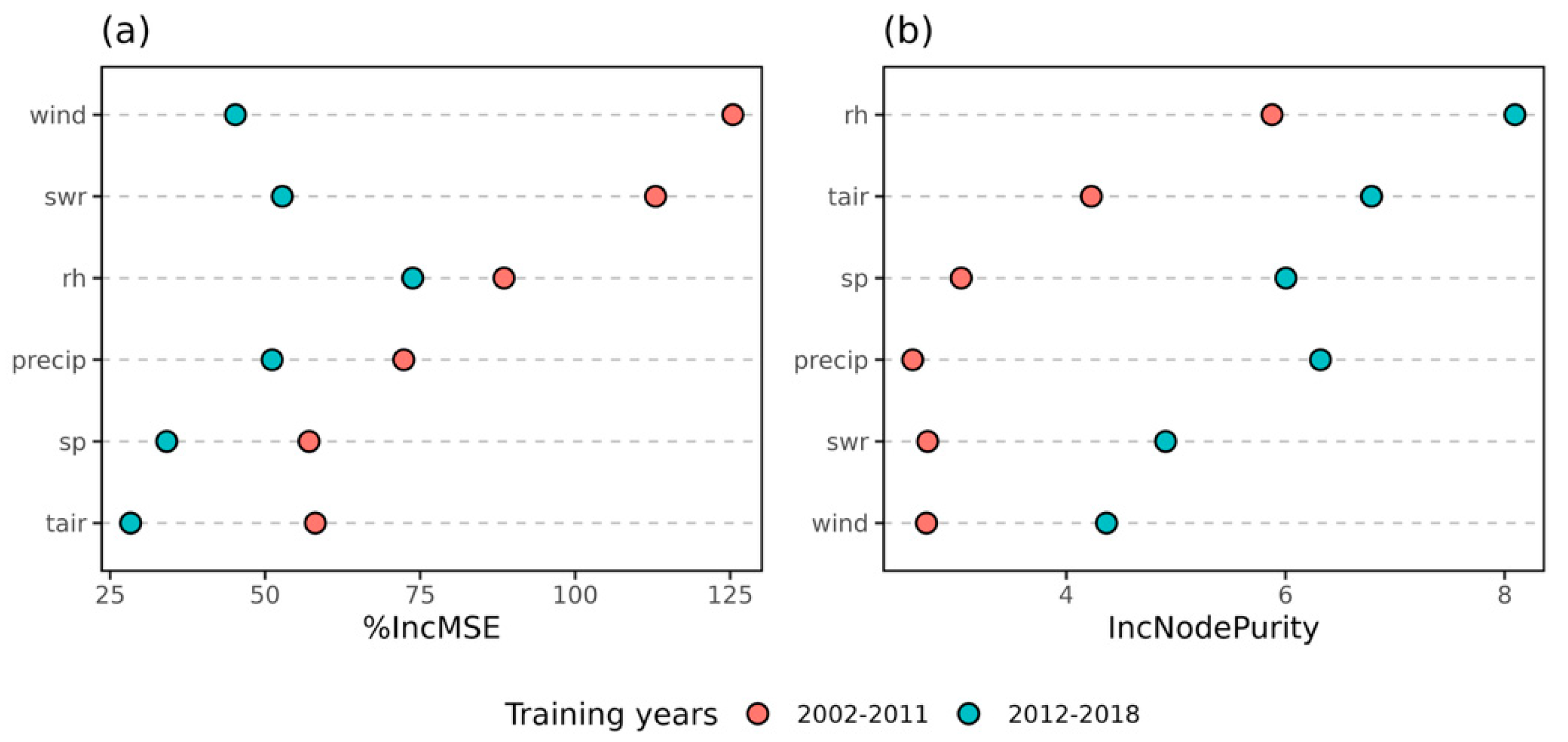
We tested six variables for their importance in predicting lightning strike rate: wind speed (m/s), relative humidity (%), shortwave radiation (W/m2), precipitation (mm), surface pressure (Pascal), and temperature (°C). Figure A1 compares variable importance between training periods. Across both training periods, relative humidity emerges as one of the most influential predictors. Shortwave radiation and wind speed show moderate importance, but their ranking differs across training periods, exhibiting a high %IncMSE for the earlier training period (2002–2011; pink points), but a lower %IncMSE for the later training period (2012–2018; blue points). Temperature is relatively low in %IncMSE but higher in IncNodePurity, potentially reflecting correlations between temperature and other predictors. Surface pressure and precipitation show lower importance across both metrics, indicating that these variables contribute less strongly to model performance.
Figure A1. Random forest results testing variable importance in predicting lightning strike rate. Metrics include (a) percent increase in mean square error (%IncMSE) and (b) increase in node impurity (IncNodePurity). Predictor variables include monthly mean wind speed (m/s), relative humidity (rh; %), shortwave radiation (swr; W/m2), precipitation (precip; mm), surface pressure (sp; Pascal), and temperature (tair; °C). Color indicates training period.
Atmosphere 17 00490 g0a1

Appendix C.2. Variable Importance for Lightning Ignition Efficiency, Pignite

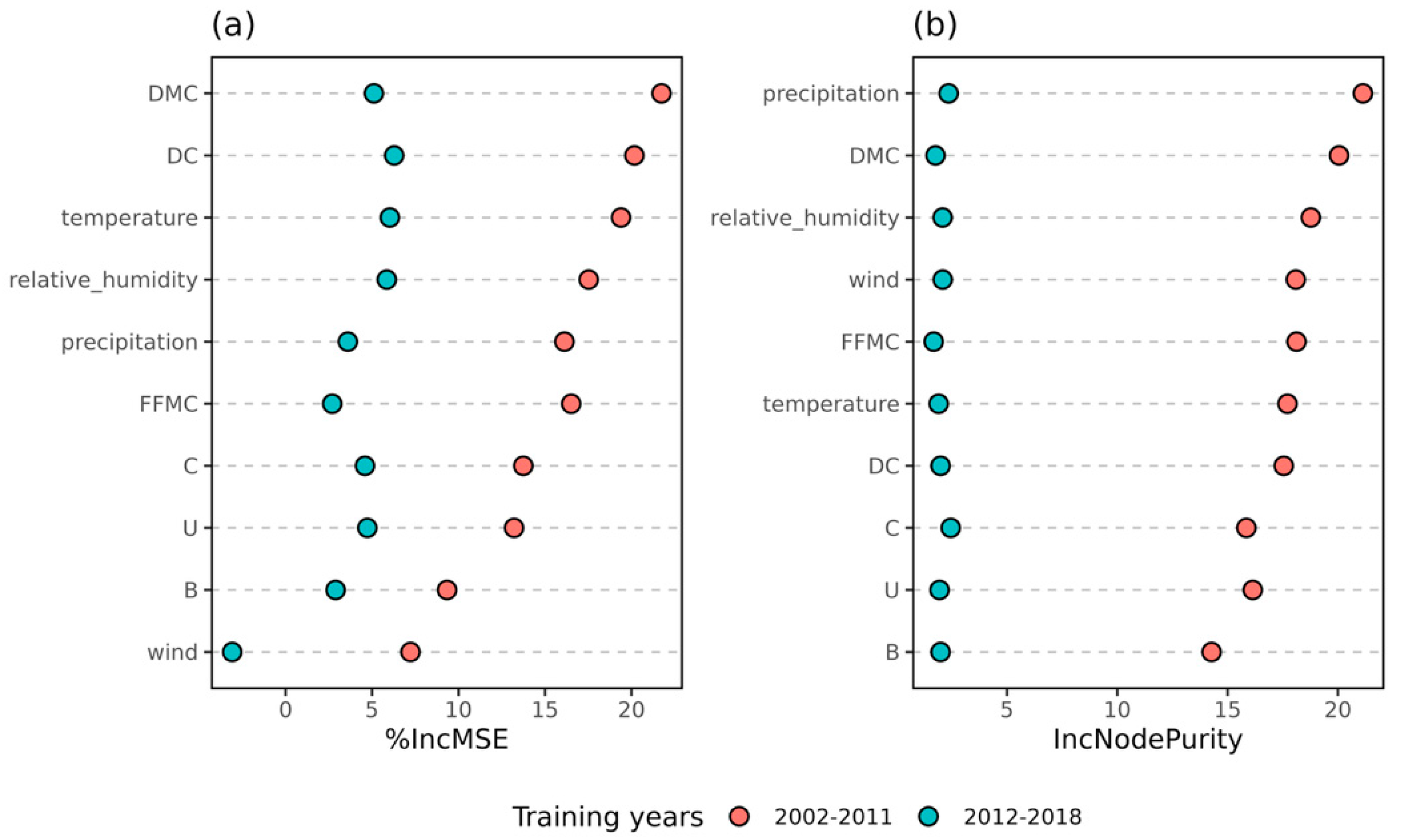
Ten variables were tested for relative importance in predicting ignition efficiency, including four climate variables: wind speed (m/s), relative humidity (%), precipitation (mm), and temperature (°C); three fuel moisture indices: fine fuel moisture code (FFMC), duff moisture code (DMC), and drought code (DC); and three vegetation cover variables: % conifer (C), % broadleaf (B), and % open land/unvegetated (U).
For models trained on the 2002–2011 dataset, several predictors show strong contributions to model performance. DMC and DC have the highest %IncMSE values, followed by temperature, relative humidity, precipitation, and FFMC. Vegetation variables (C, B, U) exhibit moderate importance, while wind has the lowest importance according to %IncMSE.
Models trained on the 2012–2018 period show substantially lower importance values across both metrics. Although temperature, relative humidity, DMC, and DC remain most influential, their absolute values are smaller during this period. Wind has slightly negative %IncMSE, indicating that it contributes little independent predictive information. Low or negative %IncMSE values likely reflect stronger correlations among predictors, which reduces permutation importance because predictive information can be taken from multiple variables.
Overall, ignition efficiency is influenced by a combination of fuel moisture conditions, temperature, relative humidity, and precipitation. The stronger importance signals observed in the 2002–2011 models likely reflect the greater range of environmental conditions captured due to a larger sample size, allowing for the random forest to more clearly identify the contribution of each predictor to ignition efficiency.
Figure A2. Random forest results testing variable importance in predicting lightning ignition efficiency. The x-axis of each plot shows (a) percent increase in mean square error (%IncMSE) and (b) increase in node impurity (IncNodePurity). The y-axes display predictor variables: monthly mean wind speed (m/s), relative humidity (rh; %), precipitation (precip; mm), temperature (tair; °C), fine fuel moisture code (FFMC), duff moisture code (DMC), and drought code (DC), % conifer cover (C), % broadleaf cover (B), and % unvegetated/openland (U). Color indicates the training period.
Atmosphere 17 00490 g0a2

References

  1. Balch, J.K.; Bradley, B.A.; Abatzoglou, J.T.; Nagy, R.C.; Fusco, E.J.; Mahood, A.L. Human-started wildfires expand the fire niche across the United States. Proc. Natl. Acad. Sci. USA 2017, 114, 2946–2951. [Google Scholar] [CrossRef]
  2. Hanes, C.C.; Wang, X.; Jain, P.; Parisien, M.-A.; Little, J.M.; Flannigan, M.D. Fire-regime changes in Canada over the last half century. Can. J. For. Res. 2019, 49, 256–269. [Google Scholar] [CrossRef]
  3. Schultz, C.J.; Nauslar, N.J.; Wachter, J.B.; Hain, C.R.; Bell, J.R. Spatial, Temporal and Electrical Characteristics of Lightning in Reported Lightning-Initiated Wildfire Events. Fire 2019, 2, 18. [Google Scholar] [CrossRef] [PubMed]
  4. Moris, J.V.; Álvarez-Álvarez, P.; Conedera, M.; Dorph, A.; Hessilt, T.D.; Hunt, H.G.P.; Libonati, R.; Menezes, L.S.; Müller, M.M.; Pérez-Invernón, F.J.; et al. A global database on holdover time of lightning-ignited wildfires. Earth Syst. Sci. Data 2023, 15, 1151–1163. [Google Scholar] [CrossRef]
  5. Scholten, R.C.; Jandt, R.; Miller, E.A.; Rogers, B.M.; Veraverbeke, S. Overwintering fires in boreal forests. Nature 2021, 593, 399–404. [Google Scholar] [CrossRef] [PubMed]
  6. Dorph, A.; Marshall, E.; Parkins, K.A.; Penman, T.D. Modelling ignition probability for human- and lightning-caused wildfires in Victoria, Australia. Nat. Hazards Earth Syst. Sci. 2022, 22, 3487–3499. [Google Scholar] [CrossRef]
  7. Shmuel, A.; Lazebnik, T.; Glickman, O.; Heifetz, E.; Price, C. Global lightning-ignited wildfires prediction and climate change projections based on explainable machine learning models. Sci. Rep. 2025, 15, 7898. [Google Scholar] [CrossRef]
  8. DeWilde, L.; Chapin, F.S. Human Impacts on the Fire Regime of Interior Alaska: Interactions among Fuels, Ignition Sources, and Fire Suppression. Ecosystems 2006, 9, 1342–1353. [Google Scholar] [CrossRef]
  9. Calef, M.P.; McGuire, A.D.; Chapin, F.S. Human Influences on Wildfire in Alaska from 1988 through 2005: An Analysis of the Spatial Patterns of Human Impacts. Earth Interact. 2008, 12, 1–17. [Google Scholar] [CrossRef]
  10. Calef, M.P.; Varvak, A.; McGuire, A.D. Differences in Human versus Lightning Fires between Urban and Rural Areas of the Boreal Forest in Interior Alaska. Forests 2017, 8, 422. [Google Scholar] [CrossRef]
  11. Veraverbeke, S.; Rogers, B.M.; Goulden, M.L.; Jandt, R.R.; Miller, C.E.; Wiggins, E.B. Lightning as a major driver of recent large fire years in North American boreal forests. Nat. Clim. Change 2017, 7, 529–534. [Google Scholar] [CrossRef]
  12. Hessilt, T.D.; Abatzoglou, J.T.; Chen, Y.; Randerson, J.T.; Scholten, R.C.; van der Werf, G.; Veraverbeke, S. Future increases in lightning ignition efficiency and wildfire occurrence expected from drier fuels in boreal forest ecosystems of western North America. Environ. Res. Lett. 2022, 17, 054008. [Google Scholar] [CrossRef]
  13. Kelly, R.; Chipman, M.L.; Higuera, P.E.; Stefanova, I.; Brubaker, L.B.; Hu, F.S. Recent burning of boreal forests exceeds fire regime limits of the past 10,000 years. Proc. Natl. Acad. Sci. USA 2013, 110, 13055–13060. [Google Scholar] [CrossRef] [PubMed]
  14. Clark, J.S. Particle motion and the theory of charcoal analysis: Source area, transport, deposition, and sampling. Quat. Res. 1988, 30, 67–80. [Google Scholar] [CrossRef]
  15. Lynch, J.A.; Clark, J.S.; Bigelow, N.H.; Edwards, M.E.; Finney, B.P. Geographic and temporal variations in fire history in boreal ecosystems of Alaska. J. Geophys. Res. Atmos. 2002, 107, FFR 8-1-FFR 8-17. [Google Scholar] [CrossRef]
  16. Sierra-Hernández, M.R.; Beaudon, E.; Porter, S.E.; Mosley-Thompson, E.; Thompson, L.G. Increased Fire Activity in Alaska Since the 1980s: Evidence From an Ice Core-Derived Black Carbon Record. J. Geophys. Res. Atmos. 2022, 127, e2021JD035668. [Google Scholar] [CrossRef]
  17. Higuera, P.E.; Brubaker, L.B.; Anderson, P.M.; Hu, F.S.; Brown, T.A. Vegetation mediated the impacts of postglacial climate change on fire regimes in the south-central Brooks Range, Alaska. Ecol. Monogr. 2009, 79, 201–219. [Google Scholar] [CrossRef]
  18. Lynch, J.; Clark, J.; Stocks, B. Charcoal production, dispersal, and deposition from the Fort Providence experimental fire. Can. J. For. Res. 2004, 34, 1642–1656. [Google Scholar] [CrossRef]
  19. Brown, J.L.; Hill, D.J.; Dolan, A.M.; Carnaval, A.C.; Haywood, A.M. PaleoClim, high spatial resolution paleoclimate surfaces for global land areas. Sci. Data 2018, 5, 180254. [Google Scholar] [CrossRef]
  20. Hakim, G.J.; Emile-Geay, J.; Steig, E.J.; Noone, D.; Anderson, D.M.; Tardif, R.; Steiger, N.; Perkins, W.A. The last millennium climate reanalysis project: Framework and first results. J. Geophys. Res. Atmos. 2016, 121, 6745–6764. [Google Scholar] [CrossRef]
  21. Kageyama, M.; Braconnot, P.; Harrison, S.P.; Haywood, A.M.; Jungclaus, J.H.; Otto-Bliesner, B.L.; Peterschmitt, J.-Y.; Abe-Ouchi, A.; Albani, S.; Bartlein, P.J.; et al. The PMIP4 contribution to CMIP6–Part 1: Overview and over-arching analysis plan. Geosci. Model Dev. 2018, 11, 1033–1057. [Google Scholar] [CrossRef]
  22. Etten-Bohm, M.; Yang, J.; Schumacher, C.; Jun, M. Evaluating the Relationship Between Lightning and the Large-Scale Environment and its Use for Lightning Prediction in Global Climate Models. J. Geophys. Res. Atmos. 2021, 126, e2020JD033990. [Google Scholar] [CrossRef]
  23. Moon, S.-H.; Kim, Y.-H. Forecasting lightning around the Korean Peninsula by postprocessing ECMWF data using SVMs and undersampling. Atmos. Res. 2020, 243, 105026. [Google Scholar] [CrossRef]
  24. Romps, D.M.; Seeley, J.T.; Vollaro, D.; Molinari, J. Projected increase in lightning strikes in the United States due to global warming. Science 2014, 346, 851–854. [Google Scholar] [CrossRef] [PubMed]
  25. Price, C.; Rind, D. What determines the cloud-to-ground lightning fraction in thunderstorms? Geophys. Res. Lett. 1993, 20, 463–466. [Google Scholar] [CrossRef]
  26. Price, C.; Rind, D. Modeling Global Lightning Distributions in a General Circulation Model. Mon. Weather Rev. 1994, 122, 1930–1939. [Google Scholar] [CrossRef]
  27. Nikolov, N.; Bothwell, P.; Snook, J. Probabilistic Forecasting of Lightning Strikes over the Continental USA and Alaska: Model Development and Verification. Fire 2024, 7, 111. [Google Scholar] [CrossRef]
  28. Bieniek, P.A.; Bhatt, U.S.; York, A.; Walsh, J.E.; Lader, R.; Strader, H.; Ziel, R.; Jandt, R.R.; Thoman, R.L. Lightning Variability in Dynamically Downscaled Simulations of Alaska’s Present and Future Summer Climate. J. Appl. Meteorol. Climatol. 2020, 59, 1139–1152. [Google Scholar] [CrossRef]
  29. Chen, Y.; Romps, D.M.; Seeley, J.T.; Veraverbeke, S.; Riley, W.J.; Mekonnen, Z.A.; Randerson, J.T. Future increases in Arctic lightning and fire risk for permafrost carbon. Nat. Clim. Change 2021, 11, 404–410. [Google Scholar] [CrossRef]
  30. Uden, C.; Clemins, P.J.; Beckage, B. Predicting Lightning from Near-Surface Climate Data in the Northeastern United States: An Alternative to CAPE. Atmosphere 2025, 16, 1298. [Google Scholar] [CrossRef]
  31. Peterson, D.; Wang, J.; Ichoku, C.; Remer, L.A. Effects of lightning and other meteorological factors on fire activity in the North American boreal forest: Implications for fire weather forecasting. Atmos. Chem. Phys. 2010, 10, 6873–6888. [Google Scholar] [CrossRef]
  32. Sedano, F.; Randerson, J.T. Multi-scale influence of vapor pressure deficit on fire ignition and spread in boreal forest ecosystems. Biogeosciences 2014, 11, 3739–3755. [Google Scholar] [CrossRef]
  33. Kasischke, E.; Williams, D.; Barry, D. Analysis of the patterns of large fires in the boreal forest region of Alaska. Int. J. Wildland Fire 2002, 11, 131–144. [Google Scholar] [CrossRef]
  34. Earth Science Data Systems; NASA. PalEON: Terrestrial Ecosystem Model Drivers for the Northeastern U.S., 0850–2010. NASA Earthdata; 16 June 2025. Available online: https://www.earthdata.nasa.gov/data/catalog/ornl-cloud-nacp-paleon-mip-1779-1 (accessed on 19 March 2026).
  35. Kumar, J.; Brooks, B.-G.J.; Thornton, P.E.; Dietze, M.C. Sub-daily Statistical Downscaling of Meteorological Variables Using Neural Networks. Procedia Comput. Sci. 2012, 9, 887–896. [Google Scholar] [CrossRef]
  36. Dawson, A.; Williams, J.W.; Gaillard, M.-J.; Goring, S.J.; Pirzamanbein, B.; Lindstrom, J.; Anderson, R.S.; Brunelle, A.; Foster, D.; Gajewski, K.; et al. Holocene land cover change in North America: Continental trends, regional drivers, and implications for vegetation–atmosphere feedbacks. Clim. Past 2025, 21, 2031–2060. [Google Scholar] [CrossRef]
  37. Pirzamanbein, B.; Lindström, J.; Poska, A.; Gaillard, M.J. Modelling Spatial Compositional Data: Reconstructions of past land cover and uncertainties. Spat. Stat. 2018, 24, 14–31. [Google Scholar] [CrossRef]
  38. Pirzamanbein, B.; Poska, A.; Lindström, J.B. Reconstruction of Past Land Cover from Pollen Data: Model Robustness and Sensitivity to Auxiliary Variables. Earth Space Sci. 2020, 7, e2018EA00057. [Google Scholar] [CrossRef]
  39. Karger, N.; Nobis, M.P.; Normand, S.; Graham, C.H.; Zimmermann, N.E. CHELSA-TraCE21k–high-resolution (1 km) downscaled transient temperature and precipitation data since the Last Glacial Maximum. Clim. Past 2023, 19, 439–456. [Google Scholar] [CrossRef]
  40. Power, M.J.; Marlon, J.R.; Bartlein, P.J.; Harrison, S.P. Fire history and the Global Charcoal Database: A new tool for hypothesis testing and data exploration. Palaeogeogr. Palaeoclimatol. Palaeoecol. 2010, 291, 52–59. [Google Scholar] [CrossRef]
  41. U.S. Department of the Interior, Bureau of Land Management (BLM). BLM AFS Impact System Lightning 1986–2012 Points, NAD83. Available online: https://fire.ak.blm.gov/predsvcs/maps.php (accessed on 7 March 2024).
  42. U.S. Department of the Interior, Bureau of Land Management (BLM). BLM AFS TOA Lightning 2012–2025 Points, WGS84. [Vector Digital Data]. Available online: https://fire.ak.blm.gov/predsvcs/maps.php (accessed on 6 October 2025).
  43. Scholten, R.C.; Veraverbeke, S.; Jandt, R.; Miller, E.A.; Rogers, B.M. ABoVE: Ignitions, Burned Area, and Emissions of Fires in AK, YT, and NWT, 2001–2018; ORNL Distributed Active Archive Center: Oak Ridge, TN, USA, 2021. [CrossRef]
  44. Hersbach, J.; Bell, B.; Berrisford, P.; Hirahara, S.; Horányi, A.; Muñoz-Sabater, J.; Nicolas, J.; Peubey, C.; Radu, R.; Schepers, D.; et al. The ERA5 global reanalysis. Q. J. R. Meteorol. Soc. 2020, 146, 1999–2049. [Google Scholar] [CrossRef]
  45. Van Wagner, C.E.; Pickett, T.L. Equations and FORTRAN Program for the Canadian Forest Fire Weather Index System. 1985. Available online: https://ostrnrcan-dostrncan.canada.ca/handle/1845/228362 (accessed on 15 March 2026).
  46. Commission for Environmental Cooperation (CEC). NALCMS. The North American Land Change Monitoring System—A Trinational Collaboration of More Than 21 Million Square Kilometers. 25 September 2024. [2005, 2010, 2015, and 2020 Raster Digital Data]. Available online: https://www.cec.org/north-american-environmental-atlas/?_atlas_keyword=land-cover (accessed on 19 December 2025).
  47. Coogan, S.C.P.; Cannon, A.J.; Flannigan, M.D. Lightning ignition efficiency in Canadian forests. Fire Ecol. 2025, 21, 34. [Google Scholar] [CrossRef]
  48. R Core Team. R: A Language and Environment for Statistical Computing; R Foundation for Statistical Computing: Vienna, Austria, 2024; Available online: https://www.R-project.org/ (accessed on 20 August 2025).
  49. Stan Development Team. RStan: The R Interface to Stan. 2024. Available online: https://mc-stan.org/ (accessed on 20 August 2025).
  50. Larjavaara, M.; Pennanen, J.; Tuomi, T.J. Lightning that ignites forest fires in Finland. Agric. For. Meteorol. 2005, 132, 171–180. [Google Scholar] [CrossRef]
  51. Friedman, J.H.; Hastie, T.; Tibshirani, R. Regularization Paths for Generalized Linear Models via Coordinate Descent. J. Stat. Softw. 2010, 33, 1–22. [Google Scholar] [CrossRef]
  52. Feller, W. The Poisson Approximation. In An Introduction to Probability Theory and Its Applications, 3rd ed.; Wiley: New York, NY, USA, 1967; Volume 1, pp. 153–154. [Google Scholar]
  53. Breiman, L. Random Forests. Mach. Learn. 2001, 45, 5–32. [Google Scholar] [CrossRef]
  54. Perkins, S.E.; Pitman, A.J.; Holbrook, N.J.; McAneney, J. Evaluation of the AR4 Climate Models’ Simulated Daily Maximum Temperature, Minimum Temperature, and Precipitation over Australia Using Probability Density Functions. J. Clim. 2007, 20, 4356–4376. [Google Scholar] [CrossRef]
  55. Hijmans, R.J. Geodata: Access Geographic Data. 2026. Available online: https://rspatial.github.io/geodata/ (accessed on 22 April 2026).
  56. Nowacki, G.J.; Spencer, P.; Fleming, M.; Brock, T.; Jorgenson, T. Unified Ecoregions of Alaska: 2001. U.S. Geological Survey 2002-297. 2003. Available online: https://pubs.usgs.gov/publication/ofr2002297 (accessed on 23 March 2026).
  57. Krause, A.; Kloster, S.; Wilkenskjeld, S.; Paeth, H. The sensitivity of global wildfires to simulated past, present, and future lightning frequency. J. Geophys. Res. Biogeosci. 2014, 119, 312–322. [Google Scholar] [CrossRef]
  58. Anderson, K. A model to predict lightning-caused fire occurrences. Int. J. Wildland Fire 2002, 11, 163–172. [Google Scholar] [CrossRef]
  59. Vant-Hull, B.; Thompson, T.; Koshak, W. Optimizing Precipitation Thresholds for Best Correlation Between Dry Lightning and Wildfires. J. Geophys. Res. Atmos. 2018, 123, 2628–2639. [Google Scholar] [CrossRef]
  60. Reap, R.M. Climatological Characteristics and Objective Prediction of Thunderstorms over Alaska. Weather Forecast. 1991, 6, 309–319. [Google Scholar] [CrossRef]
  61. Dissing, D.; Verbyla, D.L. Spatial patterns of lightning strikes in interior Alaska and their relations to elevation and vegetation. Can. J. For. Res. 2003, 33, 770–782. [Google Scholar] [CrossRef]
  62. Price, C.; Rind, D. A simple lightning parameterization for calculating global lightning distributions. J. Geophys. Res. Atmos. 1992, 97, 9919–9933. [Google Scholar] [CrossRef]
  63. Burton, C.; Betts, R.; Cardoso, M.; Feldpausch, T.R.; Harper, A.; Jones, C.D.; Kelley, D.I.; Robertson, E.; Wiltshire, A. Representation of fire, land-use change and vegetation dynamics in the Joint UK Land Environment Simulator vn4.9 (JULES). Geosci. Model Dev. 2019, 12, 179–193. [Google Scholar] [CrossRef]
  64. Mangeon, S.; Voulgarakis, A.; Gilham, R.; Harper, A.; Sitch, S.; Folberth, G. INFERNO: A fire and emissions scheme for the UK Met Office’s Unified Model. Geosci. Model Dev. 2016, 9, 2685–2700. [Google Scholar] [CrossRef]
  65. Knorr, W.; Kaminski, T.; Arneth, A.; Weber, U. Impact of human population density on fire frequency at the global scale. Biogeosciences 2014, 11, 1085–1102. [Google Scholar] [CrossRef]
  66. Nieradzik, L.P.; Haverd, V.E.; Briggs, P.; Meyer, C.P.; Canadell, J. BLAZE, a novel Fire Model for the CABLE Land-Surface Model applied to a Re-Assessment of the Australian Continental Carbon Budget. In AGU Fall Meeting Abstracts; American Geophysical Union: Washington, DC, USA, 2015; p. GC33E-1350. Available online: https://ui.adsabs.harvard.edu/abs/2015AGUFMGC33E1350N (accessed on 12 February 2026).
  67. Li, F.; Zeng, X.D.; Levis, S. A process-based fire parameterization of intermediate complexity in a Dynamic Global Vegetation Model. Biogeosciences 2012, 9, 2761–2780. [Google Scholar] [CrossRef]
  68. Arora, V.K.; Boer, G.J. Fire as an interactive component of dynamic vegetation models. J. Geophys. Res. Biogeosci. 2005, 110, G02008. [Google Scholar] [CrossRef]
  69. Melton, J.R.; Arora, V.K. Competition between plant functional types in the Canadian Terrestrial Ecosystem Model (CTEM) v. 2.0. Geosci. Model Dev. 2016, 9, 323–361. [Google Scholar] [CrossRef]
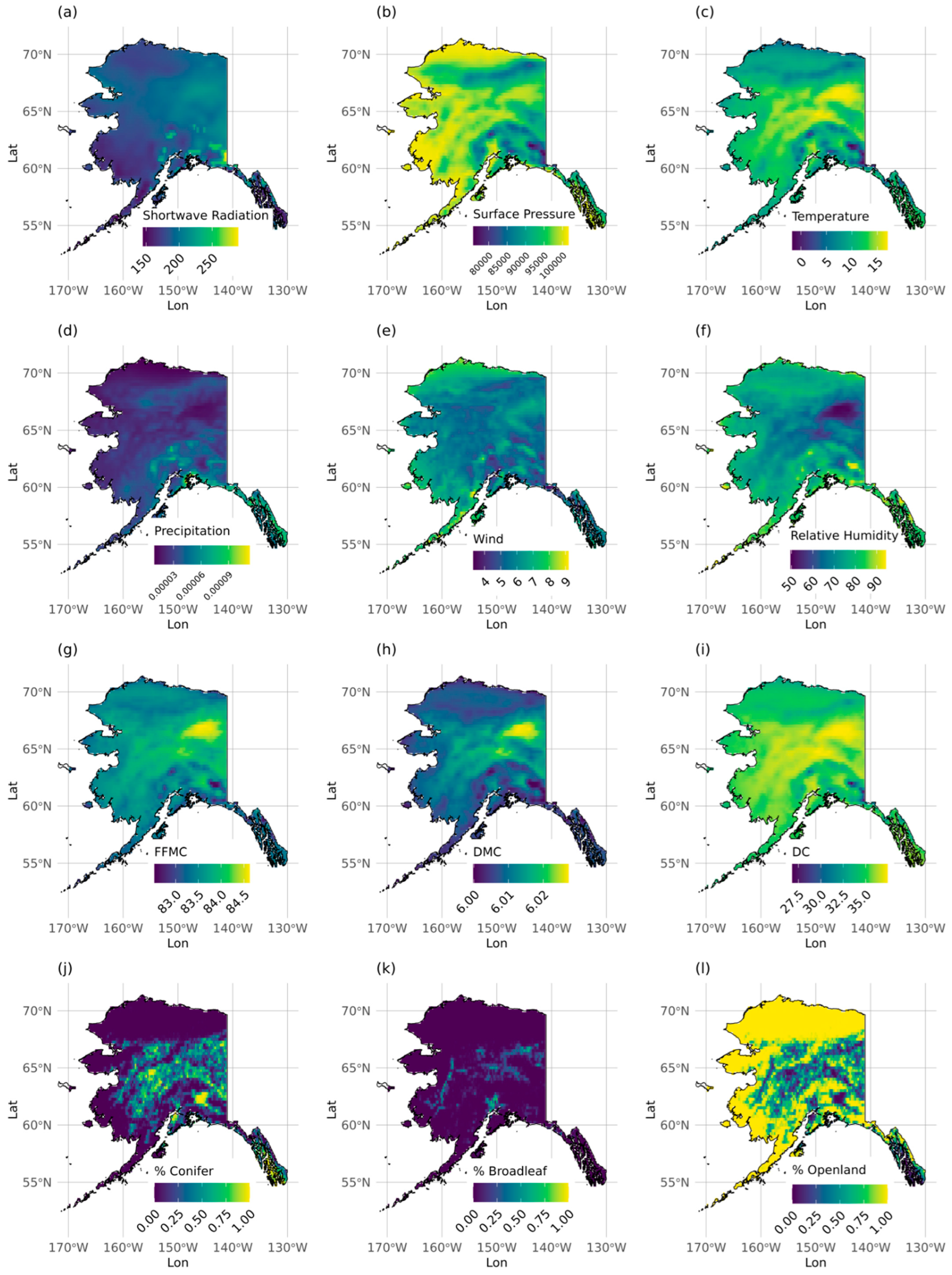
Figure 1. Mapped mean values of climate, fuel moisture, and land cover data (2002–2011). Climate data include (a) surface downward shortwave radiation (W/m2), (b) surface pressure (Pa), (c) temperature (°C), (d) total daily precipitation (m), (e) 10 m wind speed (m/s), (f) relative humidity (%). Fuel moisture codes include (g) fine fuel moisture code, (h) duff moisture code, and (i) drought code. Land cover data include (j) % land covered by coniferous vegetation, (k) % land covered by broadleaf vegetation, (l) % open land or unvegetated.
Atmosphere 17 00490 g001
Figure 2. Flow chart of methods, from input data (yellow boxes) to models (green boxes), output data (orange boxes), and performance tests (blue boxes). Models in the two left-hand columns vary according to input predictor variables, model type, and training period, with performance metrics used to select a model with the ‘best’ balance across performance metrics. The right-hand column is separated by a dashed vertical line, as it represents integration of lightning and ignition efficiency models into the fire probability model after training and testing (left-hand columns).
Atmosphere 17 00490 g002
Figure 3. Performance of lightning prediction models across predictor groups, modeling approaches, and training periods. Panels show six evaluation metrics: (a) normalized root mean square error (nRMSE), (b) correlation between observed and predicted values, (c) skill score [54], (d) spatial correlation, (e) anomaly correlation coefficient (ACC), and (f) nRMSE of anomalies. Points represent metric estimates with horizontal bars indicating 95% bootstrap confidence intervals. Predictor groups are arranged on the y-axis, with model approach represented by point color (linear model=blue, Gamma GLM = orange, Gamma Bayesian=purple) and training period represented by point shape (2002–2011 = circle, 2012–2018 = triangle). Each panel is divided into two sections: the upper facet (out-of-period test) shows performance of the near-surface Gamma GLM when parameters estimated from one period are applied to data from the alternate period, while the lower facet (in-period test) shows performance evaluated on a held-out 20% test set from the same period used for training. In panels (a,f) values on the x-axis are reversed so that better performance appears on the right (allowing consistent interpretation across all plots).
Atmosphere 17 00490 g003
Figure 4. Performance of ignition probability models across predictor groups, modeling approaches, and training periods. Panels show five evaluation metrics: (a) area under the receiver operating characteristic curve (ROC AUC), (b) area under the precision–recall curve (PR AUC), (c) Brier score, (d) calibration intercept, and (e) calibration slope. Points represent model estimates with horizontal bars indicating 95% bootstrap confidence intervals. Predictor groups are arranged on the y-axis, approach distinguished by point color (glmnet=magenta, Bayesian=orange) and training period distinguished by point shape (2002–2011 = circle, 2012–2018 = triangle). Each panel is divided into two sections: the upper facet (out-of-period test) shows performance of the climate + fuel moisture + vegetation Bayesian logistic regression when parameters estimated from one period are applied to data from the alternate period, while the lower facet (in-period test) shows performance evaluated on a held-out 20% test set from the same period used for training. In panels (a,b), higher values indicate stronger discrimination with dashed vertical lines marking no-skill thresholds (ROC AUC = 0.5; PR AUC = 1.55 × 10⁻⁴ for 2002–2011 and PR AUC = 1.89 × 10⁻⁵ for 2012–2018). Panel (c) displays Brier scores on a reversed axis so that better performance appears on the right. Panels (d,e) assess calibration: a calibration intercept of 0 indicates unbiased predictions, and a slope of 1 indicates perfectly scaled probabilities (dashed vertical lines provide a reference).
Atmosphere 17 00490 g004
Figure 5. Evaluation of predicted lightning-caused fire probabilities. (a) Reliability diagram for predicted lightning-caused fire probabilities. Predicted daily gridcell fire probabilities are grouped into ten quantile-based bins containing approximately equal number of samples. For each bin, the mean predicted probability (x-axis) is plotted against the observed frequency of fire occurrence (y-axis). The dashed 1:1 line indicates perfect model calibration. (b) Receiver operating characteristics (ROC) curve showing the tradeoff between true positive rate and false positive rate across all probability thresholds. The dashed diagonal line represents a no-skill classifier. (c) Precision-recall (PR) curve illustrating model performance under severe class imbalance. Precision measures the fraction of predicted fire days that correspond to observed fires and recall measures the fraction of observed fires captured by the model. The dashed horizontal line indicates the baseline event frequency (fire days/total days). Red points mark threshold values sampled for reference.
Atmosphere 17 00490 g005
Figure 6. Interannual variability of observed fire frequency and simulated fire probability in Alaska, 2002–2011. Yellow circles show annual mean observed fire rate (number of fire days/total number of days) with error bars representing 95% binomial confidence intervals around the annual mean fire occurrence. Blue triangles show annual mean predicted fire probability with error bars representing bootstrap 95% confidence interval of the annual mean, via resampling cells with replacement. The dotted horizontal line marks the ten-year observed mean lightning-caused fire rate (0.000067) and provides a reference for interannual anomalies.
Atmosphere 17 00490 g006
Figure 7. Mapped predictions and observations of lightning strike rates, lightning ignition efficiency, and fire occurrence in Alaska, June–August 2002–2011. The top row contains model predictions of (a) lightning strike rates, (b) ignition probability, and (c) fire probability, estimated from ERA5 climate and fuel moisture data, and NALCMS land cover data and are summarized as the mean prediction per gridcell across the ten-year period. The middle row contains summaries of observed data, including (d) mean lightning strike rate, (e) ignition rates (number of strikes that caused a fire/total number of strikes), and (f) fire rate (number of fire days/total number of days). Lightning and wildfire data come from the Alaska Lightning Detection Network and the Alaska-Yukon-Northwest Territories Fire Emissions Database. The bottom row contains per-gridcell calculations of mean bias for (g) lightning strike rate (seasonal predicted—observed strikes/km2/month) and (h) fire probability (daily predicted probability—observed 0/1 outcome). Purple gridcells indicate underprediction and orange gridcells indicate overprediction. Topographic lines downloaded using the geodata R package [55] are also displayed.
Atmosphere 17 00490 g007
Figure 8. Climate controls on modeled lightning strike rate, ignition efficiency, and lightning-caused fire probability in Alaska, 2002–2011. Heatmaps show the mean modeled response to combinations of daily near surface climate variables: temperature and relative humidity (ac), temperature and precipitation (df), temperature and wind speed (gi), relative humidity and precipitation (jl), precipitation and wind speed (mo), and relative humidity and wind speed (pr). These climate variables were selected because they are applied in both the lightning and ignition efficiency models, allowing consistent comparison of their influence across models. Columns correspond to the three modeled components: lightning strike rate (strikes/month/km2; left), ignition efficiency (center), and fire probability (right). Colors indicate the mean model prediction within quantile-based climate bins with warmer colors indicating higher predicted values.
Atmosphere 17 00490 g008
Table 1. Metrics used to test the performance of r s t r i k e , P i g n i t e , and P f i r e .
MetricTestValue Interpretation
Lightning Strike Rate, rstrike
nRMSEMagnitude of prediction error relative to observed mean0 = perfect agreement; larger values = increasing error
Pearson
Correlation
Linear co-variation between observed and predicted strike rates1 = perfect agreement; 0 = no relationship; negative = inverse relationship
S-scoreDistributional agreement; similarity of predicted and observed distributions1 = identical distributions; 0 = no overlap
Spatial CorrelationAgreement in spatial patterns of lightning activity1 = strong correspondence in geographic patterns; 0 = weak spatial agreement
Anomaly Correlation CoefficientAgreement in interannual anomalies1 = perfect, 0 = no skill, negative = inverse relationship
nRMSE of anomaliesMagnitude of error in interannual variabilityvalues < 1 = anomaly errors smaller than observed variability; values > 1 = poor reproduction of interannual variability
Ignition Efficiency, Pignite
ROC AUCRanking skill; ability to discriminate ignitions from non-ignitions1 = perfect discrimination; 0.5 = no skill
PR AUCRare-event skill; discrimination under class imbalance.higher values = better identification of true ignitions; baseline = event prevalence
Brier ScoreOverall probabilistic accuracy; mean squared error of probabilistic predictionsLower values = better performance; 0 = perfect
Calibration InterceptSystematic bias in
predicted probabilities
0 = no bias; positive values = underprediction; negative values = overprediction
Calibration SlopeCalibration of predictions1 = perfect calibration; slope < 1 = overconfidence, slope > 1 = underconfidence
Fire Probability, Pfire
ROC AUCDiscrimination1 = perfect; 0.5 = no skill
PR AUCRare-event discriminationhigher values = better identification of true ignitions; baseline = event prevalence
Disclaimer/Publisher’s Note: The statements, opinions and data contained in all publications are solely those of the individual author(s) and contributor(s) and not of MDPI and/or the editor(s). MDPI and/or the editor(s) disclaim responsibility for any injury to people or property resulting from any ideas, methods, instructions or products referred to in the content.