Article

Hailstorms That Produce Very Large Hail: What Are the Differences with Other Thunderstorms?

Forecast Area, Servei Meteorologic de Catalunya, Dr. Roux, 80, 08013 Barcelona, Spain
Atmosphere 2026, 17(5), 436; https://doi.org/10.3390/atmos17050436
Submission received: 1 March 2026 / Revised: 10 April 2026 / Accepted: 22 April 2026 / Published: 24 April 2026
(This article belongs to the Section Meteorology)

Abstract

Hail events commonly affect the Western part of Catalonia, producing damage mainly in the agricultural sector. Comparison of the weather radar data with hail pad registers at ground level allows for the diagnosis of hail severity. However, limitations using individual radar fields have led to the use of quantiles of the vertical profiles of reflectivity for a period between 12 min before and after a hailfall. These profiles combine all radar parameters, and are less sensitive to radar functioning anomalies and hailfall nature. The explored dataset was divided into severe and non-severe registers, with two subsets: one larger (90% of cases) for modeling and the second one for validating the results. Results indicate a better estimation of severe hail, but the number of false alarms with non-severe cases was still high. In consequence, future work should focus on minimizing false alarms using more restrictive profile groups. The purpose of the study is the application of a real-time tool for improving surveillance tasks which provides better discrimination between severe and non-severe hail occurrences.

1. Introduction

According to the World Meteorological Organization Cloud Atlas, hail is any regular or irregular ice particle falling from a thunderstorm with a diameter exceeding 5 mm. It is one of the most damaging phenomena in different regions around the world [1], including the United States of America (USA) [2], Canada [3], Argentina [4], Europe [5], China [6], and Australia [7], among others. Based on [8], hail damage has increased in recent years and is comparable in annual losses to hurricanes in the USA. Hailstorms affect agriculture, buildings, cars, infrastructures, and even people, with events producing injuries and even some casualties [9,10,11,12]. Large hail-producing thunderstorms have large dimensions and very intense updrafts [1,13,14]; however, their mid-term forecasting (between one and two days in advance) and hail size diagnosis is still challenging [15,16,17]. The main cause is the difficulty in reproducing the large number of internal processes occurring inside the thunderstorms [18], which includes electrification [19], wet and dry growth of graupel and hailstones [20,21,22,23], and very strong updrafts and other thermodynamic physics [24].
Several authors [9,10,25] show the relationship between hailstone size and effects at ground level, generally using weather radar information and comparisons with direct observations. This research shows a high dependance of observations on population density. Other studies compared the radar fields with economic losses, provided by insurance [26,27]. Size and shape, among other atmospheric factors, help to increase the terminal fall speed of the stones, increasing the impact on the hit surface [28]. This means that in the case of non-naturally shaped hailstones (non-spheric ones), the fall speed does not increase. However, naturally shaped hailstones (spheric ones) fall at lower speeds [29,30]. Marcos et al. [31] shows that hail pads are very useful for measuring this impact in real situations.
The previous paragraphs presented the importance of weather radar and hail pads in diagnosing hail inside a thunderstorm and estimating the hail size distribution [32,33]. The two systems are highly valuable in understanding hailstorm evolution. Hail pad networks [34] provide very useful data in large areas (ranging between 100 and 1000 km2) with a short distance between pads. Each hail pad provides the distribution of stones, providing information about the size and energy of impact. The disadvantage is that information acquisition is delayed with respect to the event occurrence (more than one day, even six months for the final processed data) [32]. Therefore, it is not useful for real-time surveillance tasks. In contrast, weather radar fields provide volumetric information inside the thunderstorm that allows us to infer the dynamic behavior of the cloud [17]. However, ground surface hail size estimation is not always accurate because of different system limitations [35]. The comparison of both sources, which can be made when hail pad data is available, helps to calibrate the different radar parameters and provide more precise maps of hail size occurrence and distribution [25].
Limitations of the weather radar in providing realistic estimations of hail size at ground level [1] have led to the development of different radar products and the identification of signatures that have helped in the diagnosis of the phenomenon at different levels, depending on the system technology and the product characteristics. There are a wide range of products with diverse degrees of complexity, depending on the level of process. Ortega [36] evaluated multiple radar products in a project comparing those fields with ground observations in the United States, and the study is one of the best guides regarding identifying the most common fields. Cică et al. [37] conducted similar research in Romania, but used less products. Pilorz et al. [38] performed a comparison between different versions of volumetric radar products with different configurations based on different temperature thresholds associated with hail formation in Poland.
The products included in the previous studies are [13,15,16,17,36,37,38]: the maximum expected size of hail (MESH), probability of hail (POH) and probability of severe hail (POSH), the echo tops for the 50 and 60 dBZ thresholds (or the maximum height where echoes exceed those thresholds in a radar column), the vertically integrated liquid (VIL, or the integration of the reflectivity at all vertical levels of a radar column) and VIL density (the VIL divided by the echo top), ground reflectivity, vertically integrated ice (VII, similar to VIL, but only for the echoes between heights with temperatures between −10 and −40 °C), the hail kinetic energy (HKE), composite reflectivity at low levels, and the maximum reflectivity. The products that were better correlated with hail observation were those that considered the vertical development of the thunderstorm. There are other variables obtained from dual polarization [39], which theoretically provides better results than single polarization. Finally, Allen et al. [1] summarized some signatures observed in radar fields that can be associated with hail occurrence due to the interaction of the beam with the stones (TBSS, three-body scattering signature) or the region (BWE, bounded weak echo) with null reflectivity values caused by the strong updrafts in hailstorms. However, it is very difficult to relate these signatures with exact sizes at ground level.
Hail in Catalonia occurs recursively each year, with a high variability with respect to the number of cases, the maximum size occurred, the monthly distribution, or the spatial distribution along the territory during a year [40]. Aran et al. [41] showed how a favorable synoptic configuration is the basis for hail occurrence, but it is not a definitive condition. The properties of the stones also vary depending on the season [42,43,44], with a clear dependence on thermodynamic conditions. The region has suffered notable hail events, some of them reported in [12] or [45]. The Servei Meteorological de Catalunya (SMC) put in operation the first version of the Lightning Jump algorithm (a signature of a sudden rise in total lightning in a thunderstorm, associated with a strong updraft and the production of hail) in 2020 [46]. Because of the high impact on agriculture [43], there is an operational hail pad network in the Western region to analyze the events that produce the most damage in agricultural regions [32,43]. Rigo and Llasat [13] made an initial analysis using the life cycle of thunderstorms to observe the evolution of different radar parameters (echo top, VIL, and reflectivity), indicating that the faster the thunderstorms grew, the higher the probability of hail occurrence.
Bearing in mind recent events with hail sizes exceeding 10 cm (the largest size that the SMC has ever noticed in the area) and that some of those thunderstorms had dimensions never observed before in the region (with tropical-like dimensions), using weather radar and hail pad data, the principal question that this study tries to answer is if there is any relationship between thunderstorm dimensions and hail observed at ground level. To achieve this, the study considered all impacted hail pads from the period 2016–2025 and evaluated the evolution of different radar parameters (VIL density, reflectivity and echo top) on the ground over a 24 min interval. Once the first comparison was made, the next step was to use vertical profile reflectivity to define thresholds useful for the diagnosis in real time.

2. Area of Study, Data and Methodology

2.1. Area of Study

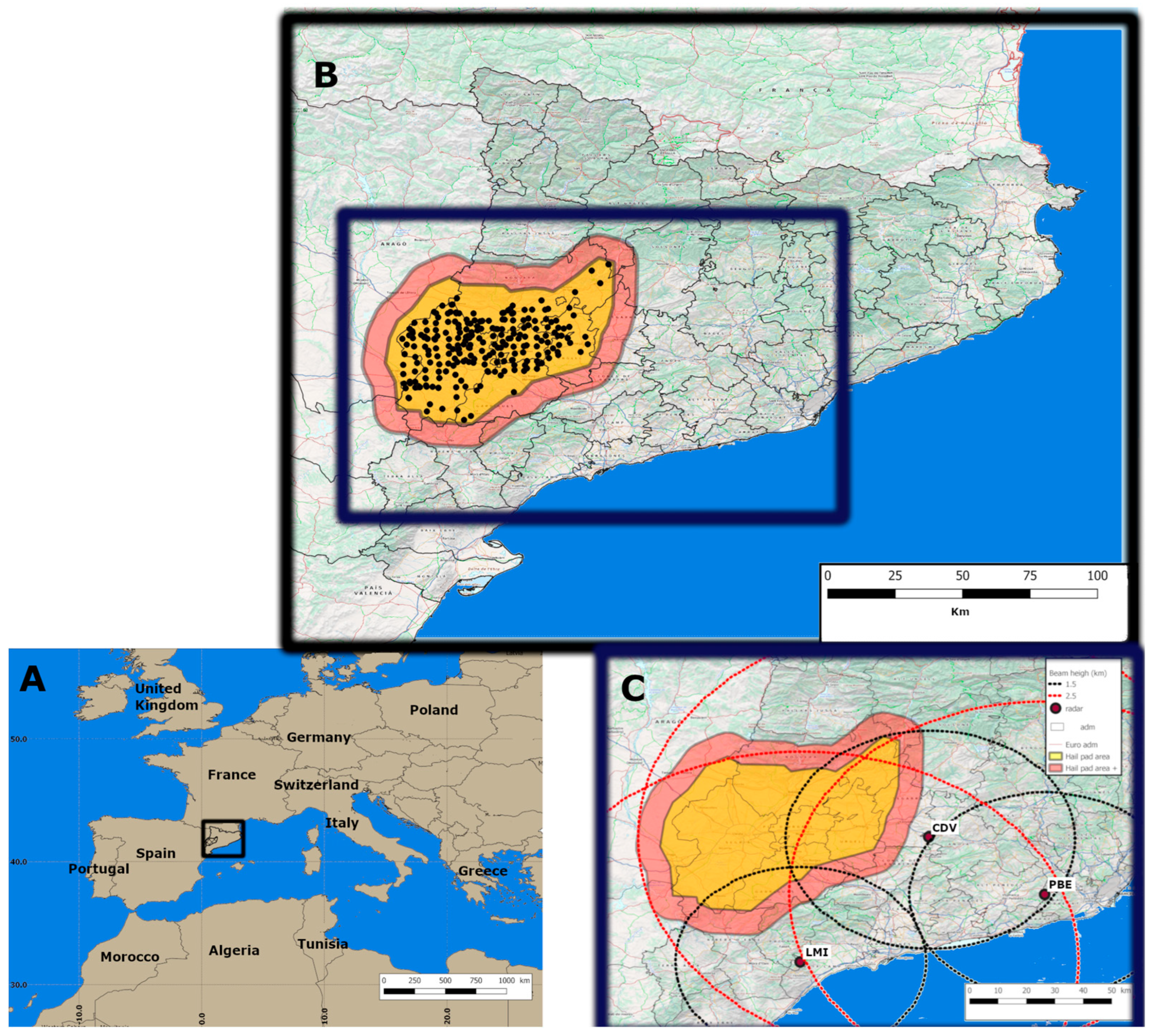
The area of study includes a flat region in western Catalonia (NE of the Iberian Peninsula, black rectangle in Figure 1A), with a total size of 4240 km2 (yellow region in Figure 1B). The region was selected because it has a hail pad network with available data since 2001 [41]. The region was enlarged with a buffered section (red area in the same figure) to include radar information for all the selected events. Therefore, the total size of the study region was 7200 km2. The area of study is well known for high-impact hailstorms that affect the agricultural industry, with irrigated and rainfed crops depending on water management [32,34,41,43,45]. In this case, it has been selected because ground hail observations (from the hail pads) and volumetric weather data (Figure 1C) are both available for a long period of time (in this case, the 10 years from 2016 to 2025).

2.2. Data

The preliminary data source for the selection of events comes from the records of each hail pad of the network shown in Figure 1B. The network consists of more than 150 elements (depending on the campaign) which are distributed in a semi-regular grid with 4 km between each sensor. This high resolution provides a very good distribution of the hailfalls that occurred in the region. In the present study, the unique considered data is the maximum hail size, but other characteristics are measured (mean size, kinetic energy, and density, among others). The selection of the maximum hail size responds to two points. First, as the purpose of the study is to extend the results to the rest of the Catalan area, where hail pads are not available. Second, maximum hail size is usually reported by most spotters and in general can be correlated with damage. The network is managed by the ADV-Terres de Ponent (Lleida, Catalonia, Spain) organization, in collaboration with the SMC and the University of Leon (Leon, Spain). The hail pads are not electronic but homemade Styrofoam plaques manufactured to a measurement of 31 cm, which were changed due to the following causes: robbery, hail, isolation, and animal damage, among others.
Weather radar data is from the XRAD (Radar network of the SMC). Figure 1C shows how the area is well covered by three radars (lowest beam height below 2.5 km—red dashed line—for two of them and the third not exceeding 3.5 km, a height that allows adequate characterization of the thunderstorms in three dimensions [44]). The products have a time resolution of 6 min and are a composition of the maximum value at each point. The used fields are the volumetric reflectivity, with a grid size of 2 × 2 × 1 km, and CAPPI (Constant Altitude Plan Position Indicator) heights between 1 and 10 km. In addition, the TOP45 (or maximum echo top for a reflectivity threshold of 45 dBZ) and the VIL density are used for comparisons with each ground observation (both products had a grid size of 1 × 1 km).

2.3. Methodology

Figure 2 shows the scheme of the methodology considered in the research. Each hail pad register (including the date, longitude, latitude, and the maximum diameter of the stone) was searched for the time with the highest maximum reflectivity value over the hail pad coordinates in the 6 min volumetric radar composite. The time of the highest maximum reflectivity for the lowest three kilometers of the volumetric scan is defined as the time of the hailfall. This method has limitations because of different factors, such as radar reflectivity attenuation mainly at low levels [47,48], the effects of some phenomena associated with the thunderstorm (e.g., horizontal wind or wind shear [38]), or simply the direction of the hailfall [49]. However, according to different authors, this technique is the simplest and most efficient in the majority of cases, with distance errors of less than 2 km and time gaps of less than 10 min [16,17,36,49].
The next step was to calculate the maximum reflectivity (equivalent to the intensity of the thunderstorm), the VIL density (the measure of the water content in the cloud) and the TOP45 (the vertical development of the more intense nucleus of the thunderstorm) for the period between 12 min before and 12 min after the time of the hailfall, with a 6 min gap. This period is similar to the one used in previous research [16,34]. In addition, it is worth noting that the selection of zero time using the maximum reflectivity at the lowest radar levels is not contradictory to using volumetric radar information to characterize the complete dimensions of the hailstorm during the period of fall. The 6 min values of each variable have been estimated for a radius of 5 km to have a more accurate measurement of the thunderstorm dimensions. The next step of the process was to conduct a comparison of those parameters for the two types of hail registers—non-severe (below 2 cm of diameter) and severe—for 1086 registers between 2016 and 2025. Finally, these results were compared with the vertical profiles of reflectivity for the area surrounding the hail pad to identify the pattern associated with each type of hailstone size. To make the analysis reliable, the database was divided into two groups: 90% of cases were used for calibrating the model (for both categories, severe and non-severe), while the rest were used for validating the results. The validation was made using the classical skill scores: POD (Probability of Detection), FAR (False Alarm Ratio) and CSI (Critical Succes Index) [50].

3. Results

3.1. Selection of the Events

The dataset consists of 1443 registers of hail distributed in 120 events and proceeding from 174 different hail pads. Data was collected only between April and September (although some October events are available). The period of analysis comprises the years 2016 to 2025 (sixty months in total). The most hit hail pad registered 20 cases (indicating that the pad was hit in 1.1% of the days), with a mean value of 6.2 hail events per plaque. The event with the largest number of hit hail pads was 19 April 2025 (60), while the mean value is 9.1 plaques per event. A total of 6 days registered hail in 40 or more hail pads (28 May 2016 (54), 11 May 2017 (44), 27 June 2017 (41), 29 April 2018 (53), 20 July 2018 (55), and the 19 April 2025 (60)). These values are examples of the irregularity of hailfall in the region, in terms of the number of hail pads hit (extension of the event) and of seasonality.

3.2. Categorization of the Observations

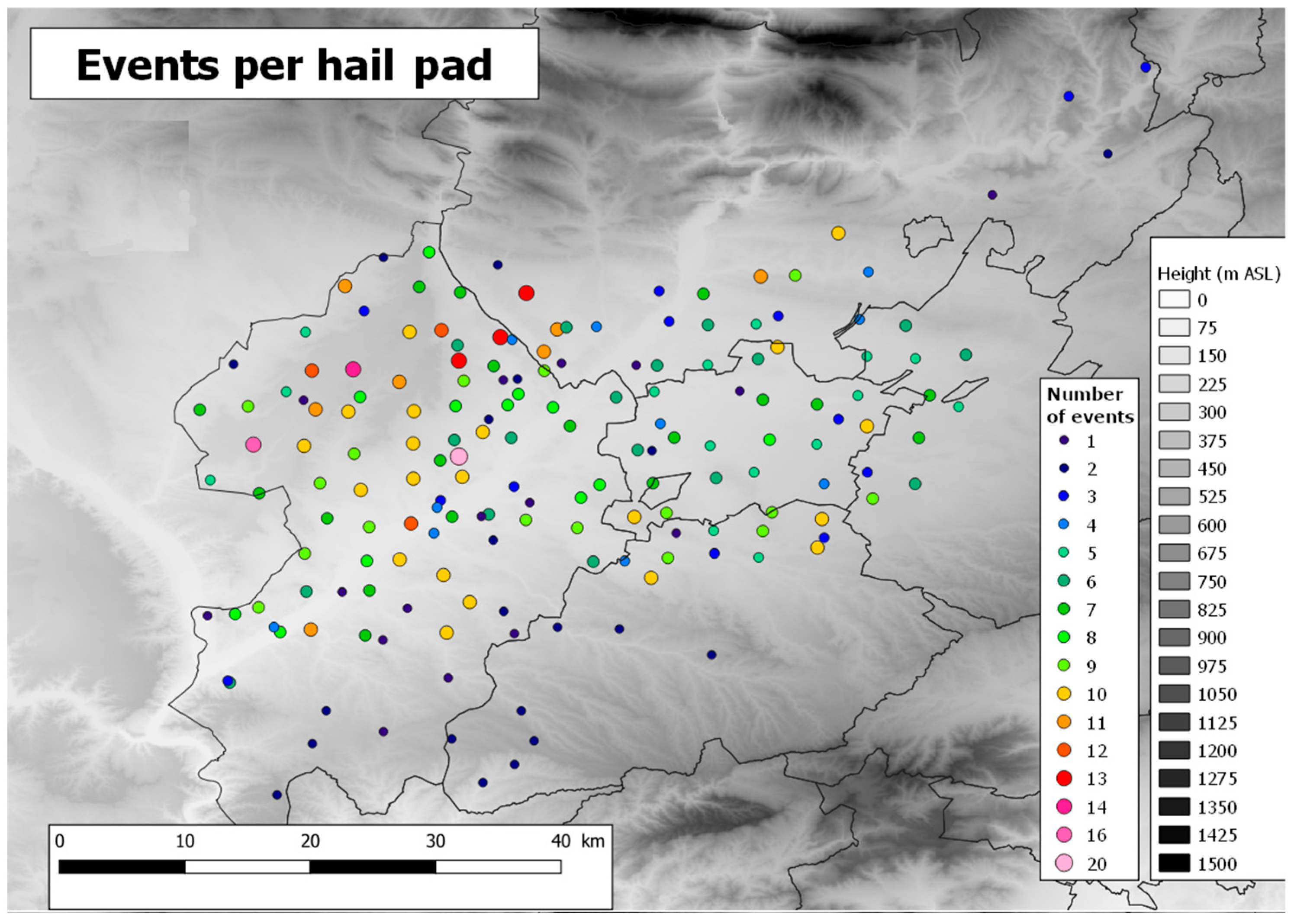
Moving to the types of observations (non-severe and severe), there is a high difference between both in the case of the number of registers and how they were distributed throughout the area of interest. Figure 3 presents all the cases (merging severe and non-severe) and shows how there were a major number of events per pad in the western and northern regions. On the other hand, southern and eastern regions had a smaller number of hail events.
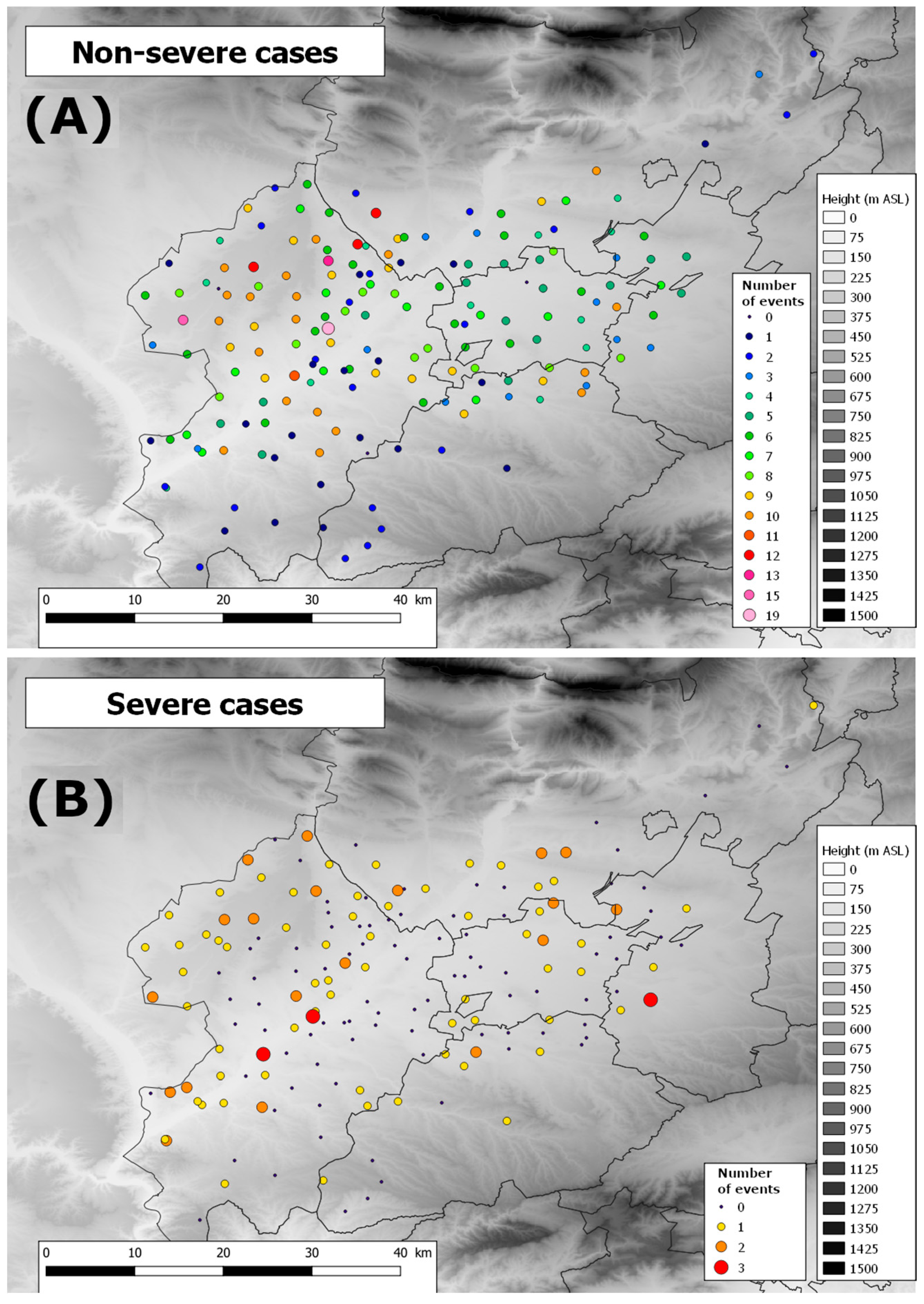
In the case of the two categories (Figure 4), non-severe hail events (panel A) have a similar configuration to the general one, indicating that most cases are of this type and affect the same regions. However, severe events (panel B), which are less frequent, are still common (two events) in the north-eastern region. Furthermore, the central and southern areas present infrequent and non-severe registers in most pads.

3.3. Weather Radar Variables: Discrimination Between Hail Sizes

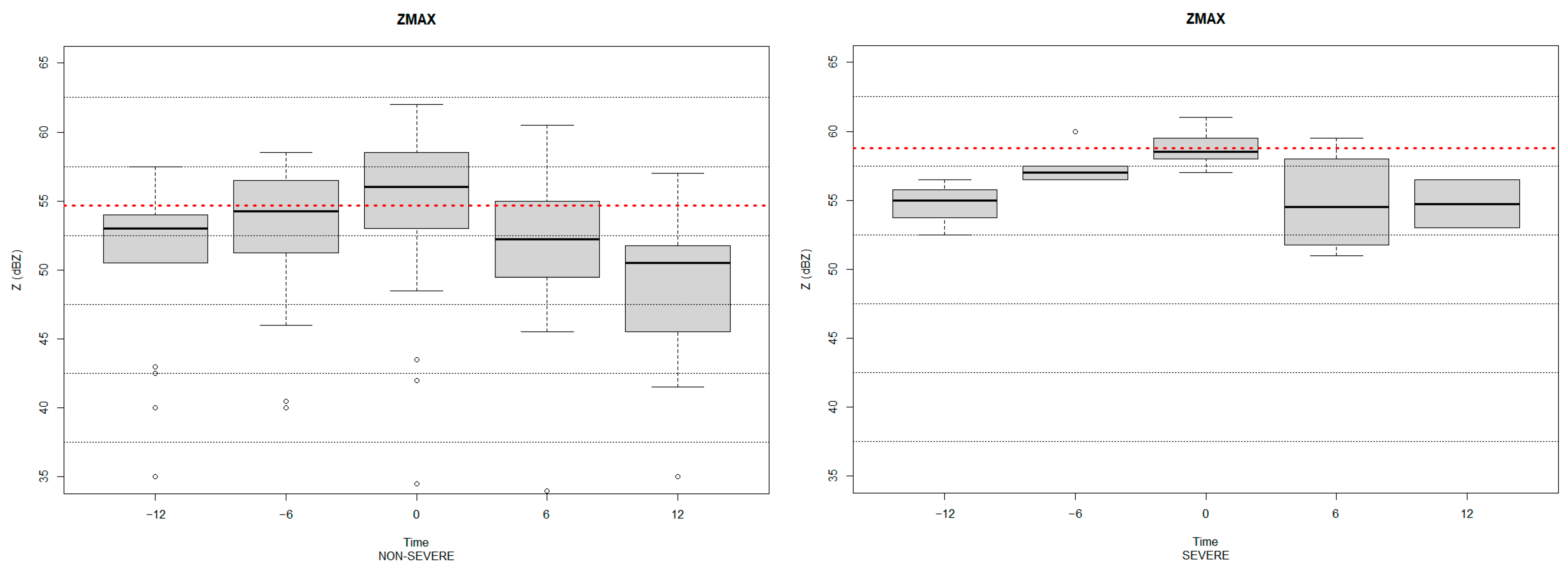
The purpose of this research is to identify differences in the behavior of the radar variables corresponding to the period of hailfall on the hail pad (from 12 min prior to the maximum reflectivity of the point to the 12 min after). Each one of the three radar variables represents a different characteristic of the hailstorm. The first one, the maximum reflectivity, is equivalent to the intensity of precipitation associated with the thunderstorm. Figure 5 shows the differences between non-severe (left) and severe (right) cases. First, it is important to consider that both sets contain a different number of cases, with non-severe registers being more frequent than severe cases (978 non-severe cases compared to 108 severe observations). To make the analysis more statistically reliable, both sets were split into two sub-groups, as described in Section 2. The first one (with 90% of the cases) was used to identify the pattern and thresholds, and the second one to validate the results. Furthermore, the Bonferroni correction [51] was applied to assess the statistical significance of differences observed in the two samples.
In any case, the following points can be deduced from the image: first, severe cases of distribution are more compact, with less dispersion. In the same way, there are no outliers in the lower limit, as happens with non-severe distribution. Lastly, the values for the five time measurements are always higher in the case of severe hailfalls, with a mean dBZ value of 58 compared to 55 for non-severe cases. If we pay attention to the time when the maximum reflectivity occurs during the selected period (Table 1), the distribution is very similar for both categories, with a peak at the time of the hailfall, and some residual cases with the maximum prior to the hailfall. In any case, the maximum reflectivity occurred after zero time.
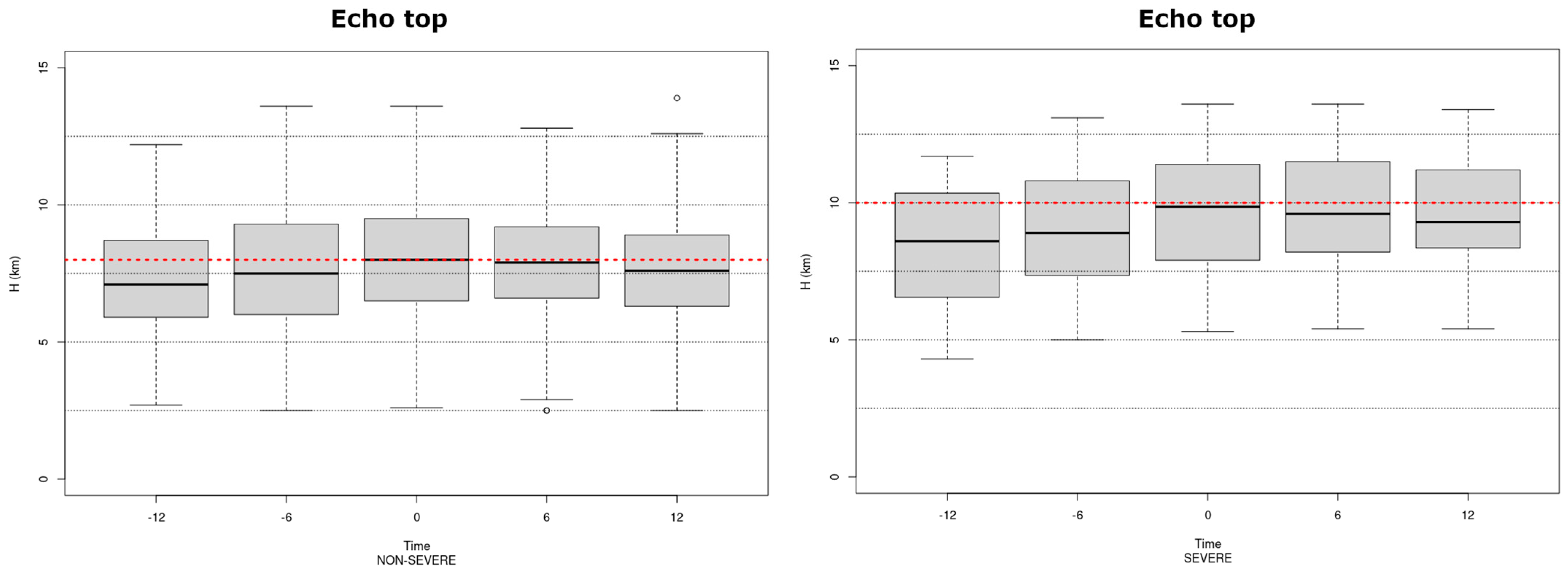
In the case of the echo top (of 45 dBZ), which is indicative of the vertical development of the more intense nucleus inside the hailstorm, the differences are also evident between non-severe and severe cases (Figure 6). In the first case, the boxes are similar at all moments, with a slight increase until the hailfall, followed by a subtle decrease after that time. In the case of severe registers, the echo top has more differences between all the boxes, indicating that the core reached the maximum development at the time of hail occurrence. The values are at all moments between 1 and 2 km higher than in the case of non-severe events. In the same vein, the mean value is 2 km higher for severe events (10 km as opposed to 8 km). A different behavior with respect to the maximum reflectivity is found in the occurrence of the maximum value (Table 1). Both the non-severe and severe cases have again the maximum echo top occurring during zero time. Another difference with reflectivity is that the distribution is more regular, with a higher percentage across all moments different to the hailfall time.
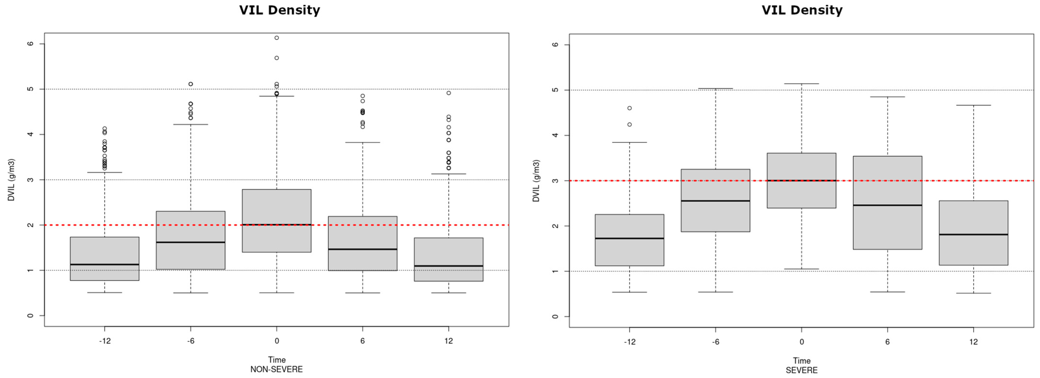
Lastly, VIL density (a measure of the water quantity inside the cloud) has a similar behavior to maximum reflectivity (Figure 7), but with wider boxes (larger dispersion of the data set respecting the mean value). In any case, the severe cases have a mean of 1 g/m3 more than non-severe cases. In this case, the distributions present sharp increases and decreases during the period, with a clear peak at the hailfall time. Table 1 shows that more than 45% of the hailfalls had a maximum value of VIL density at zero time for both categories.
Applying a simple thresholding method to the second sample of each variable (maximum reflectivity, top, and vil density) based on the mean value of the first sample, skill scores were calculated (POD, FAR and CSI) [50]. Results (Table 2) show that POD values are not bad (closer to 1 than 0), but, on the other hand, false alarms are elevated (more than 70% of cases for all variables).

3.4. Examples of Thunderstorms That Produce Large Hailstones

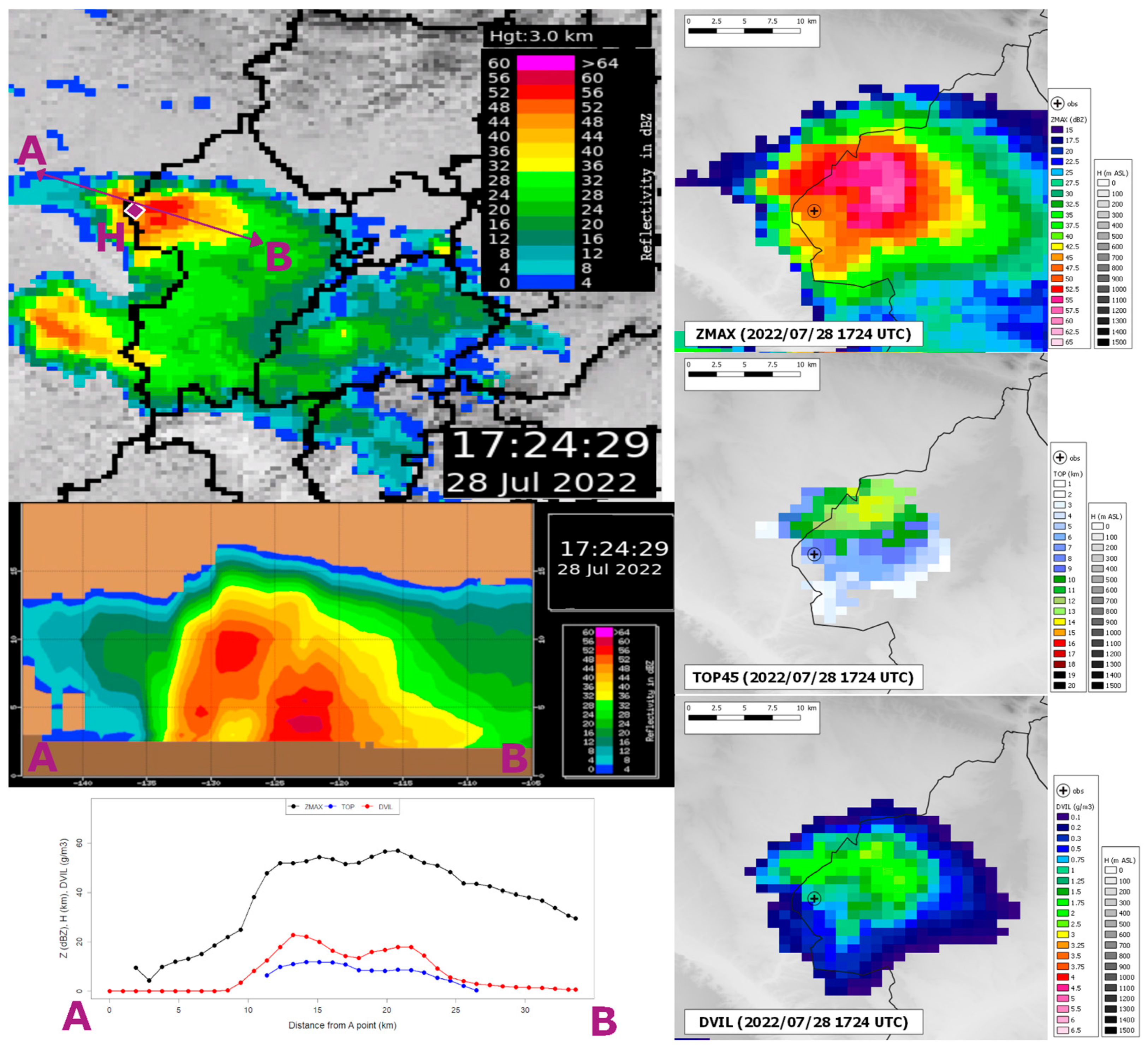
To obtain a conceptual model of severe hailstorms, some examples have been selected to reproduce different behaviors. First, it is important to understand the physical meaning of each field. To illustrate this, Figure 8 shows an example of a real case that occurred on the afternoon of 28 July 2022. Images in the left panel present the horizontal and vertical sections of a hailstorm that produced severe hail in the region (for instance, at point H in the top-left panel). The right panel contains a magnified view of the different used products for the same thunderstorm at the same time (17:24 UTC): from top to bottom, respectively, are the maximum reflectivity (ZMAX), echo top (45 dBZ, or TOP45), and vil density (DVIL). Although the structure of the thunderstorm is similar in all three figures, each one has some particularities: the location of the maximum is not the same and there is a high dependance on the vertical development of the storm in the case of TOP45, as well as for DVIL. These differences can be explained by the left and bottom middle panels (vertical section across points A to B, and the profiles of the different variables across the line): there are two vertical columns, one more developed at high levels (closer to point A) and the other with very high values of reflectivity at low levels, with lower values at high levels. In this example, ZMAX (black line) is higher for the right structure, while TOP45 (blue line) and DVIL (red line) show the opposite (higher for the left structure).
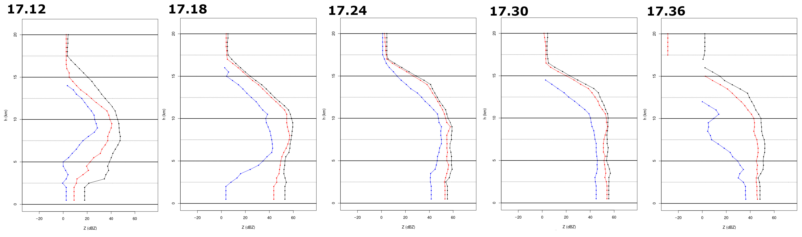
The evolution of the vertical profile of reflectivity (Figure 9) over the hailfall (“H” point in Figure 8) and the 5 km radius (considering the quantiles of 50 (blue), 90 (red), and 99 (black)) allows us to understand how the thunderstorm evolved between the 12 min prior and the 12 min after the event (17:24 UTC). It can be observed how, before the hailfall, the largest reflectivity values (near 50 dBZ) are observed at a height close to 8 km; meanwhile, the lowest level of reflectivity is near 20 dBZ. During the approach of the thunderstorm to the point of observation, reflectivity rises at all levels, but the maximum is still at a high level. At 17:24 UTC (the estimated time of the hailfall), reflectivity curves reach the highest values at all levels, but at 17:30 it can be observed how the blue curve reduces in dimension, mainly at levels between 10 and 15 km. Finally, at 17:36 all the curves decrease, indicating that the thunderstorm has finished its hail activity over the observation point.
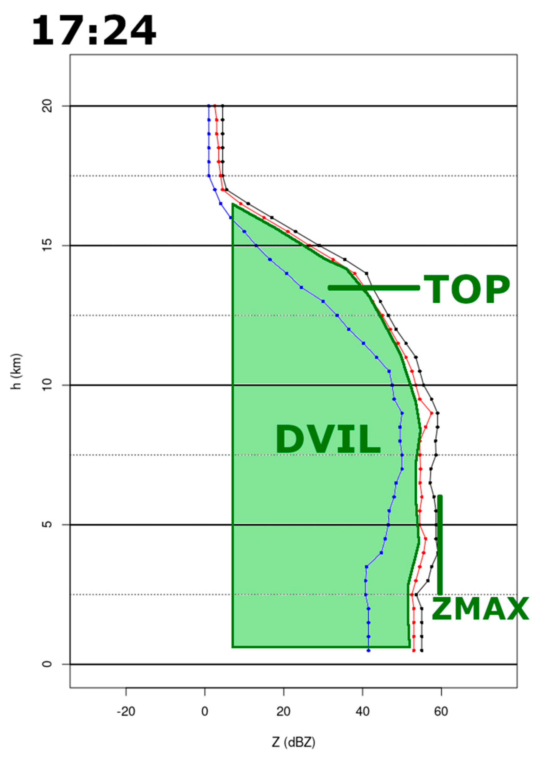
As aforementioned, the selected radar variables have a strong relationship with the hailstorm structure. To demonstrate this, it is possible to infer the radar variables (ZMAX, TOP45, and DVIL) from these curves, as Figure 10 shows. The maximum reflectivity corresponds to the right limit of the black curve, while TOP45 is the Y point when the same curve is crossing the X value of 45. Finally, the VIL density is equivalent to the area of reflectivity exceeding 0 dBZ (green area).
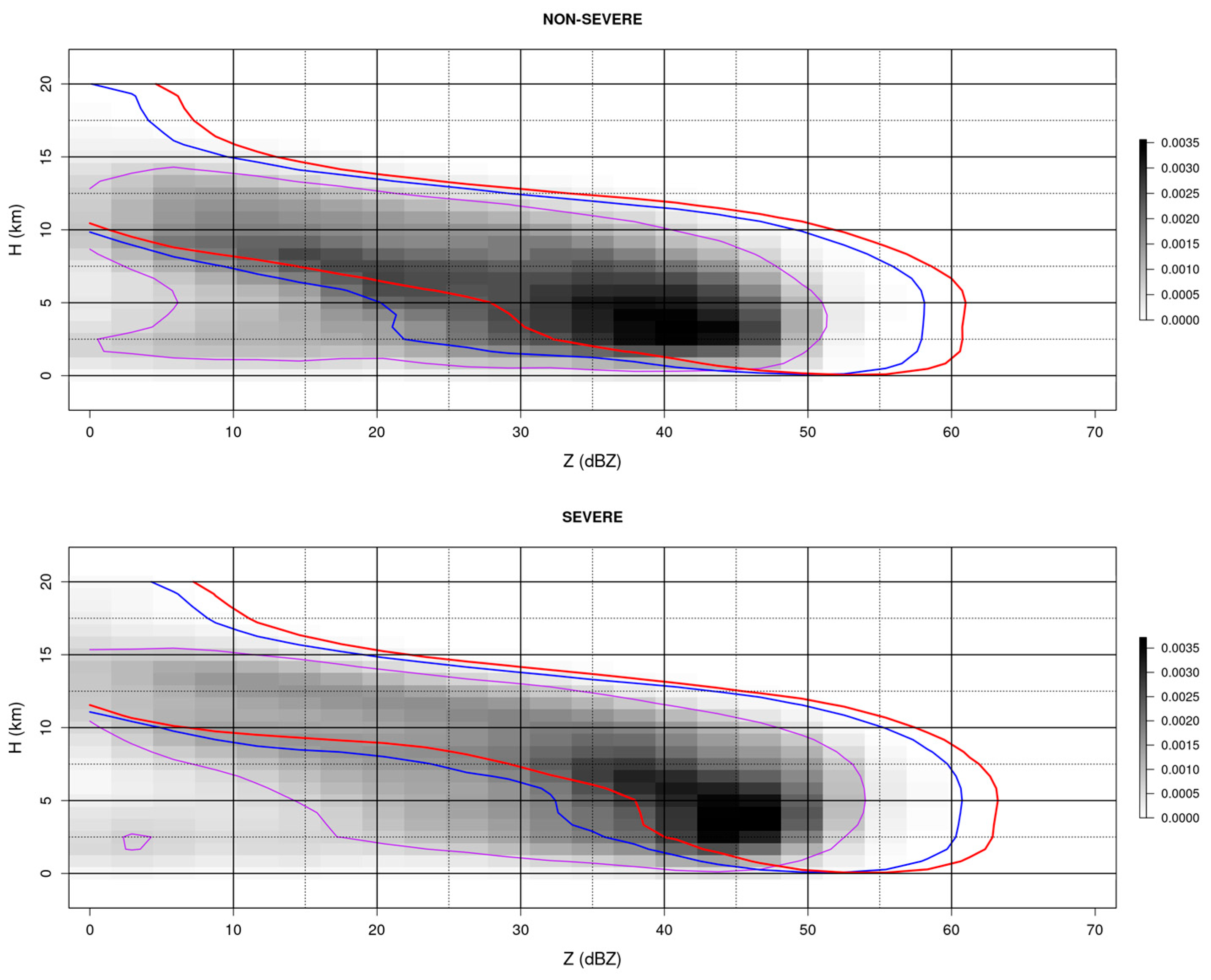
Continuing with the differences between both categories, comparing all the curves of the cases with non-severe or severe observations (Figure 11), it is possible to appreciate how the core reflectivity value (the more intense part of the thunderstorm) shows a displacement to the right (higher reflectivity values) in the case of the second category (severe hailstones). In the case of severe registers, there is a decrease in the number of lower reflectivity values at lower levels. This fact can be appreciated in the displacement of the percentile curves (mainly the 50 one, purple color) to the right (left bottom part of the chart). The same displacement in the right top part is an indicator that there are more pixels with high reflectivity values at higher levels.
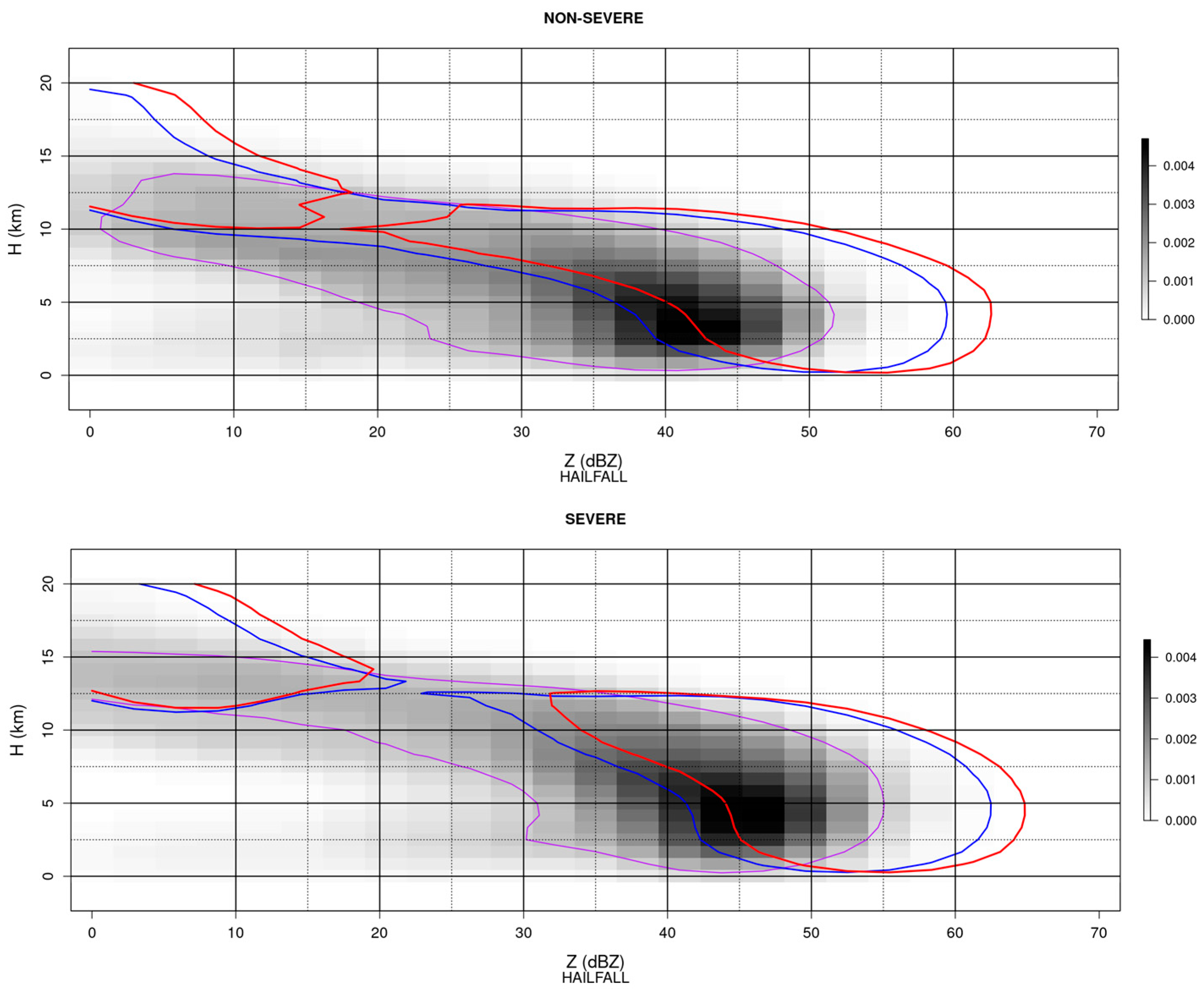
This difference is still more evident in the case when only the time of the hailfall is considered (Figure 12). Therefore, it is more important to have the shape of the curves rather than the radar parameter values themselves because of the limitations that can occur in some cases associated with the radar information or the nature of the hailstorm, as cited previously.
Finally, Figure 13 shows how the life cycle of the hailstorm over those points with non-severe hail (the two top panels) shows, across the same period, smaller areas of the vertical profile of reflectivity than for severe hail registers. These differences are more evident during the first three steps (from 12 min before the hailstorm to the instant of the event), while for the later images the differences are not as clear. Therefore, the estimation of the area can provide a signature to discriminate between both types of hail.
From the information relating to the vertical profile of reflectivity previously stated, or explored during Figure 10, Figure 11, Figure 12 and Figure 13, we tried to develop a real-time tool that estimates the 50, 90, and 99 percentiles and determines the probability of hail. The testing process is discussed in the next section.

3.5. Identification of Thresholds and Validation

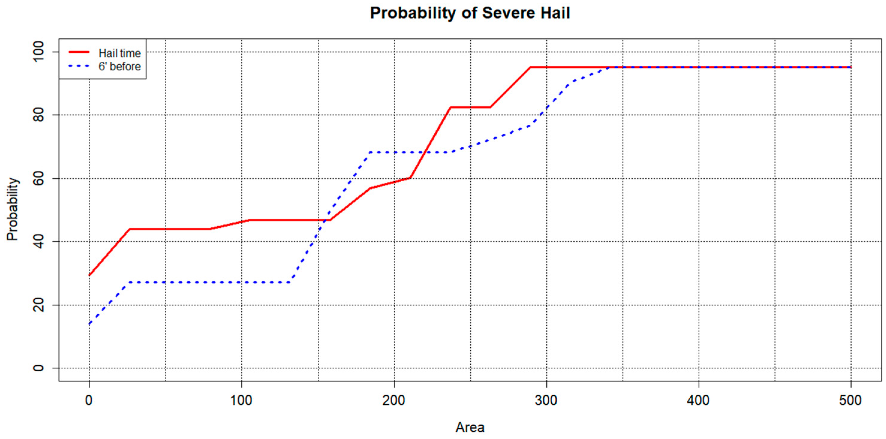
The two datasets (severe and non-severe events) of VPR curves were split into two groups: the first one (with 90% of the samples) was used to determine the values of the threshold for the green area obtained from Figure 10. The area values range from 0 to 500, and are shown in Figure 14. The second group (the 10% not considered previously) was used for validating the results, using the classical skill scores POD, FAR and CSI [50]. The curve was estimated from the time of the hailfall and the 6 min before the event. It was determined by comparing the values of the non-severe and severe cases for each area interval (considering intervals of 25 values). It can be observed that there are two breakpoints: the first one, at 150, delineates all values below this point as cases that can be considered non-severe. The second one is at 300, demarcates all cases over this value as severe. Between these two limits, the probability of severe hail increases notably with the area.
Table 3 shows the results of the skill scores for the time 6 min prior to the hailstorm and zero time. Compared to the results observed in Table 2 (for the Zmax, TOP and DVIL variables), FARs are similar in both cases, but the Probability of Detection and the Critical Succes Index improve. A future task to improve the results of this analysis would be to include the shape of the area, considering the information provided by Figure 11 and Figure 12, with the distribution of the values in the area (that is, displaced or not to the top-right). In any case, these results made the application of the technique interesting in real time. The 2026 hail campaign will act as an evaluator for the results obtained in this experimental period.
The operational tool considers all areas with pixels where VIL density exceeds a minimum value of 0.5 g/m3 with a size larger than 10 km2, to avoid spurious signals. The VPR technique is applied to all the pixels in the region, selecting closer to 5 km, and then measuring the quantiles 50, 90, and 99. The areas of those quantiles are associated with the curve of probability in diagnosing the severity of the hail.

4. Discussion

The discrimination using weather radar variables between those hailstorms that produce severe or non-severe hail is still a topic of interest. This is because some issues are nowadays still unsolved: problems with radar providing the correct values of reflectivity with the largest hailstones [1,15,35], the variability of the hail size depending also on internal factors [2,16,17,18,19], and the relationship between radar variables and ground registers [3,4,5,6,7]. Most comparisons between radar variables and hail pad observations [13,15,17,36,37] are made directly.
The first part of the study consists of searching for a threshold or set of thresholds that fit each possible category. The selected variables (maximum reflectivity, echo top, and VIL density) run operationally at the SMC in real time and are used to diagnose hail. As many previous studies found, it has some limitations that can affect the real-time diagnosis of severe hail. The seasonality of the hail type and size and the changing atmospheric conditions [25,42] imply that similar radar values can provide different ground observations [33,37,38]. Coinciding with previous studies, the results obtained in the current research indicate that in general, the largest radar parameter values (on average) coincide with the highest hail size, but there are exceptions. These exceptions coincide with the attenuation of the radar signal at lower levels produced by the large hail. Furthermore, estimations tend to produce many false alarms for non-severe cases, probably caused by the seasonality and the radar grid size.
To reduce the number of cases that are misidentified, this paper focuses on the use of the integration of several vertical profiles of reflectivity around a hail register. The area from the curve of reflectivity exceeding 0 dBZ combines the information from the three radar parameters used before (maximum reflectivity, VIL density, and echo top). These parameters have been considered in previous research [13,15,16,17,24,37,38], indicating that those and other parameters provide individually good results in diagnosing large hail in thunderstorms. In fact, some of the previous works assumed that it was necessary to combine some of them. To ensure that the errors produced by the distance or the time to the hail at ground level are minimized, it has been used in all profiles that were closer than 5 km to the point of the hail pad.
Using the curves for all the parts of a hailstorm has provided good results to discriminate against different categories of hail in the same event, observed in various hail pads. The individual and global analyses of these curves compared with the hail pad registered allow us to observe that the areas from the profiles in cases of severe hail are larger than those of non-severe hail.
This technique allows us to better observe hailstorm behavior (e.g., when the storm collapses and the probability of hail increases). In addition, it has improved the Probability of Detection, but there are still false alarms. Therefore, the algorithm must be tuned to the present campaign to apply some restrictions on the current method. One of the possible solutions would be to consider a minimum number of valid profiles to make the calculations, but this possibility should be better analyzed. Future work should also consider the development of real-time automatic warnings of severe hail.

5. Conclusions

Hailstorms produce large amounts of damage yearly, which has notably increased in recent years in different regions around the world. Individual products have severe flaws in diagnosing different types of hail, even in the same event. Using a combination of hail pads and weather radar variables, this research has focused on using multiple vertical profiles of reflectivity to combine the information of some of those variables (maximum reflectivity, echo top, and VIL density).
The combined charts from a ten-year period plus a visual analysis of a concrete event with different types of registers (non-severe and severe hail) showed promising results, with the possibility of implementing real-time automatic warnings. All the severe hail registers were correctly diagnosed with the new combined product (while individual fields underestimate some cases). POD and CSI improve with the new technique, but FARs (false alarms) are only slightly lower (0.75 to 0.70). Therefore, the main limitation is the overestimation of some non-severe hail cases. Finally, the tool will run during the 2026 hail season to test the potential applicability of the results.

Funding

This research received no external funding.

Institutional Review Board Statement

Not applicable.

Informed Consent Statement

Not applicable.

Data Availability Statement

The data presented in this study are available on request from the corresponding author due to internal processes applied to the raw data, which are not publicly available.

Acknowledgments

The author wants to thank the Servei Meteorologic de Catalunya, ADV-Terres de Ponent, and the University of Leon for the different types of data provided.

Conflicts of Interest

The author declares no conflicts of interest.

Abbreviations

The following abbreviations are used in this manuscript.
ZMAXMaximum reflectivity
DVILVIL Density
TOPEcho top for a certain reflectivity threshold
MESH Maximum Expected Size of Hail
POSHProbability of Severe Hail
SMCServei Meteorologic de Catalunya
VILVertically Integrated Liquid
VIIVertically Integrated Ice
HKEHail Kinetic Energy
POHProbability of Hail
TBSS Three-Body Scattering Signature
BWEBounded Weak Echo
XRAD Radar Network of the SMC
CAPPI Constant Altitude Plan Position Indicator

References

  1. Allen, J.T.; Giammanco, I.M.; Kumjian, M.R.; Punge, H.J.; Zhang, Q.; Groenemeijer, P.; Kunz, M.; Ortega, K. Understanding hail in the Earth system. Rev. Geophys. 2020, 58, e2019RG000665. [Google Scholar] [CrossRef]
  2. Allen, J.T.; Tippett, M.K. The characteristics of United States hail reports: 1955–2014. E-J. Sev. Storms Meteorol. 2015, 10, 1–31. [Google Scholar] [CrossRef]
  3. Etkin, D.; Brun, S.E. A note on Canada’s hail climatology: 1977–1993. Int. J. Climatol. J. R. Meteorol. Soc. 1999, 19, 1357–1373. [Google Scholar] [CrossRef]
  4. Mezher, R.N.; Doyle, M.; Barros, V. Climatology of hail in Argentina. Atmos. Res. 2012, 114–115, 70–82. [Google Scholar] [CrossRef]
  5. Hulton, F.; Schultz, D.M. Climatology of large hail in Europe: Characteristics of the European Severe Weather Database. Nat. Hazards Earth Syst. Sci. 2024, 24, 1079–1098. [Google Scholar] [CrossRef]
  6. Li, X.; Zhang, Q.; Zou, T.; Lin, J.; Kong, H.; Ren, Z. Climatology of hail frequency and size in China, 1980–2015. J. Appl. Meteorol. Climatol. 2018, 57, 875–887. [Google Scholar] [CrossRef]
  7. Raupach, T.H.; Soderholm, J.S.; Warren, R.A.; Sherwood, S.C. Changes in hail hazard across Australia: 1979–2021. npj Clim. Atmos. Sci. 2023, 6, 143. [Google Scholar] [CrossRef]
  8. Prein, A.F.; Holland, G.J. Global estimates of damaging hail hazard. Weather Clim. Extrem. 2018, 22, 10–23. [Google Scholar] [CrossRef]
  9. Púčik, T.; Castellano, C.; Groenemeijer, P.; Kühne, T.; Rädler, A.T.; Antonescu, B.; Faust, E. Large hail incidence and its economic and societal impacts across Europe. Mon. Weather Rev. 2019, 147, 3901–3916. [Google Scholar] [CrossRef]
  10. Palencia, C.; Berthet, C.; Massot, M.; Castro, A.; Dessens, J.; Fraile, R. On the individual calibration of hailpads. Atmos. Res. 2007, 83, 493–504. [Google Scholar] [CrossRef]
  11. Battaglia, M.; Lee, C.; Thomason, W.; Fike, J.; Sadeghpour, A. Hail damage impacts on corn productivity: A review. Crop Sci. 2019, 59, 1–14. [Google Scholar] [CrossRef]
  12. Farnell, C.; Batalla, E.; Rigo, T.; Pineda, N.; Sole, X.; Mercader, J.; Martin-Vide, J. Reanalysis of giant hail event in Catalonia (NE of the Iberian Peninsula). Atmos. Res. 2023, 296, 107051. [Google Scholar] [CrossRef]
  13. Rigo, T.; Llasat, M.C. Forecasting hailfall using parameters for convective cells identified by radar. Atmos. Res. 2016, 169, 366–376. [Google Scholar] [CrossRef]
  14. Klaus, V.; Krause, J. Investigating hailstorm updrafts and nowcasting hail size using a novel radar-based updraft detection. Weather Forecast. 2024, 39, 1795–1815. [Google Scholar] [CrossRef]
  15. Blair, S.F.; Laflin, J.M.; Cavanaugh, D.E.; Sanders, K.J.; Currens, S.R.; Pullin, J.I.; Cooper, D.T.; Deroche, D.R.; Leighton, J.W.; Fritchie, R.V.; et al. High-Resolution Hail Observations: Implications for NWS Warning Operations. Weather Forecast. 2017, 32, 1101–1119. [Google Scholar] [CrossRef]
  16. Blair, S.F.; Deroche, D.R.; Boustead, J.M.; Leighton, J.W.; Barjenbruch, B.L.; Gargan, W.P. A radar-based assessment of the detectability of giant hail. E-J. Sev. Storms Meteorol. 2011, 6, 1–30. [Google Scholar] [CrossRef]
  17. Ortega, K.L.; Krause, J.M.; Ryzhkov, A.V. Polarimetric radar characteristics of melting hail. Part III: Validation of the algorithm for hail size discrimination. J. Appl. Meteorol. Climatol. 2016, 55, 829–848. [Google Scholar] [CrossRef]
  18. Kumjian, M.R.; Lombardo, K.; Loeffler, S. The evolution of hail production in simulated supercell storms. J. Atmos. Sci. 2021, 78, 3417–3440. [Google Scholar] [CrossRef]
  19. Jayaratne, E.R.; Saunders, C.P.R. The interaction of ice crystals with hailstones in wet growth and its possible role in thunderstorm electrification. Q. J. R. Meteorol. Soc. 2016, 142, 1809–1815. [Google Scholar] [CrossRef]
  20. Phillips, V.T.; Khain, A.; Benmoshe, N.; Ilotoviz, E. Theory of time-dependent freezing. Part I: Description of scheme for wet growth of hail. J. Atmos. Sci. 2014, 71, 4527–4557. [Google Scholar] [CrossRef]
  21. Ziegler, C.L.; Ray, P.S.; Knight, N.C. Hail growth in an Oklahoma multicell storm. J. Atmos. Sci. 1983, 40, 1768–1791. [Google Scholar] [CrossRef]
  22. Farnell Barqué, C.; Rigo, T.; Martin-Vide, J.; Úbeda, X. Internal structure of giant hail in a catastrophic event in Catalonia (NE Iberian Peninsula). Front. Environ. Sci. 2024, 12, 1479824. [Google Scholar] [CrossRef]
  23. Farley, R.D. Numerical modeling of hailstorms and hailstone growth. Part II: The role of low-density riming growth in hail production. J. Appl. Meteorol. Climatol. 1987, 26, 234–254. [Google Scholar] [CrossRef]
  24. Manzato, A.; Riva, V.; Tiesi, A.; Miglietta, M. Observational analysis and simulations of a severe hailstorm in northeastern Italy. Q. J. R. Meteorol. Soc. 2020, 146, 3587–3611. [Google Scholar] [CrossRef]
  25. Farnell, C.; Rigo, T.; Martin-Vide, J. Application of cokriging techniques for the estimation of hail size. Theor. Appl. Climatol. 2018, 131, 133–151. [Google Scholar] [CrossRef]
  26. Brown, T.M.; Pogorzelski, W.H.; Giammanco, I.M. Evaluating hail damage using property insurance claims data. Weather Clim. Soc. 2015, 7, 197–210. [Google Scholar] [CrossRef]
  27. Fonseca-Cerda, M.d.S.; de Moel, H.; van Ederen, D.; Schmid, T.; Wouters, L.; Aerts, J.C.J.H.; Botzen, W.J.W.; Haer, T. Hailstorm prediction and loss assessment using high-resolution hazard and claims data. Atmos. Res. 2026, 329, 108501. [Google Scholar] [CrossRef]
  28. Dieling, C.; Smith, M.; Beruvides, M. Review of impact factors of the velocity of large hailstones for laboratory hail impact testing consideration. Geosciences 2020, 10, 500. [Google Scholar] [CrossRef]
  29. Heymsfield, A.; Szakáll, M.; Jost, A.; Giammanco, I.; Wright, R. A comprehensive observational study of graupel and hail terminal velocity, mass flux, and kinetic energy. J. Atmos. Sci. 2018, 75, 3861–3885. [Google Scholar] [CrossRef]
  30. Theis, A.; Borrmann, S.; Mitra, S.K.; Heymsfield, A.J.; Szakáll, M. A wind tunnel investigation into the aerodynamics of lobed hailstones. Atmosphere 2020, 11, 494. [Google Scholar] [CrossRef]
  31. Marcos, J.L.; Sánchez, J.L.; Merino, A.; Melcón, P.; Mérida, G.; García-Ortega, E. Spatial and temporal variability of hail falls and estimation of maximum diameter from meteorological variables. Atmos. Res. 2021, 247, 105142. [Google Scholar] [CrossRef]
  32. Rigo, T.; Farnell, C. A Comparison between Radar Variables and Hail Pads for a Twenty-Year Period. Climate 2024, 12, 158. [Google Scholar] [CrossRef]
  33. Sánchez, J.L.; Fraile, R.; De La Madrid, J.L.; De La Fuente, M.T.; Rodríguez, P.; Castro, A. Crop damage: The hail size factor. J. Appl. Meteorol. Climatol. 1996, 35, 1535–1541. [Google Scholar] [CrossRef]
  34. Sánchez, J.L.; Gil-Robles, B.; Dessens, J.; Martin, E.; Lopez, L.; Marcos, J.L.; Berthet, C.; Fernández, J.T.; García-Ortega, E. Characterization of hailstone size spectra in hailpad networks in France, Spain, and Argentina. Atmos. Res. 2009, 93, 641–654. [Google Scholar] [CrossRef]
  35. Trapero, L.; Bech, J.; Rigo, T.; Pineda, N.; Forcadell, D. Uncertainty of precipitation estimates in convective events by the Meteorological Service of Catalonia radar network. Atmos. Res. 2009, 93, 408–418. [Google Scholar] [CrossRef]
  36. Ortega, K.L. Evaluating multi-radar, multi-sensor products for surface hailfall diagnosis. Electron. J. Sev. Storms Meteorol. 2018, 13, 1–36. [Google Scholar] [CrossRef]
  37. Cică, R.; Burcea, S.; Bojariu, R. Assessment of severe hailstorms and hail risk using weather radar data. Meteorol. Appl. 2015, 22, 746–753. [Google Scholar] [CrossRef]
  38. Pilorz, W.; Zięba, M.; Szturc, J.; Łupikasza, E. Large hail detection using radar-based VIL calibrated with isotherms from the ERA5 reanalysis. Atmos. Res. 2022, 274, 106185. [Google Scholar] [CrossRef]
  39. Ryzhkov, A.V.; Kumjian, M.R.; Ganson, S.M.; Zhang, P. Polarimetric radar characteristics of melting hail. Part II: Practical implications. J. Appl. Meteorol. Climatol. 2013, 52, 2871–2886. [Google Scholar] [CrossRef]
  40. Rigo, T.; Farnell, C. A Summary of Hail Events during the Summer of 2022 in Catalonia: A Comparison with the Period of 2013–2021. Remote Sens. 2023, 15, 1012. [Google Scholar] [CrossRef]
  41. Aran, M.; Pena, J.; Torà, M. Atmospheric circulation patterns associated with hail events in Lleida (Catalonia). Atmos. Res. 2011, 100, 428–438. [Google Scholar] [CrossRef]
  42. Farnell, C.; Rigo, T.; Heymsfield, A. Shape of hail and its thermodynamic characteristics related to records in Catalonia. Atmos. Res. 2022, 271, 106098. [Google Scholar] [CrossRef]
  43. Aran, M.; Sairouni, A.; Bech, J.; Toda, J.; Rigo, T.; Cunillera, J.; Moré, J. Pilot project for intensive surveillance of hail events in Terres de Ponent (Lleida). Atmos. Res. 2007, 83, 315–335. [Google Scholar] [CrossRef]
  44. Rigo, T.; Farnell Barqué, C. Evaluation of the radar echo tops in Catalonia: Relationship with severe weather. Remote Sens. 2022, 14, 6265. [Google Scholar] [CrossRef]
  45. García-Ortega, E.; Fita, L.; Romero, R.; López, L.; Ramis, C.; Sánchez, J.L. Numerical simulation and sensitivity study of a severe hailstorm in northeast Spain. Atmos. Res. 2007, 83, 225–241. [Google Scholar] [CrossRef]
  46. Rigo, T.; Farnell, C. Characterisation of thunderstorms with multiple lightning jumps. Atmosphere 2022, 13, 171. [Google Scholar] [CrossRef]
  47. Borowska, L.; Ryzhkov, A.; Zrnić, D.; Simmer, C.; Palmer, R. Attenuation and differential attenuation of 5-cm-wavelength radiation in melting hail. J. Appl. Meteorol. Climatol. 2011, 50, 59–76. [Google Scholar] [CrossRef]
  48. Féral, L.; Sauvageot, H.; Soula, S. Hail detection using S- and C-band radar reflectivity difference. J. Atmos. Ocean. Technol. 2003, 20, 233–248. [Google Scholar] [CrossRef]
  49. Hohl, R.; Schiesser, H.H.; Aller, D. Hailfall: The relationship between radar-derived hail kinetic energy and hail damage to buildings. Atmos. Res. 2002, 63, 177–207. [Google Scholar] [CrossRef]
  50. Wilks, D.S. Statistical Methods in the Atmospheric Sciences, 3rd ed.; Academic Press: Oxford, UK, 2011. [Google Scholar]
  51. Kędra, M. Altered precipitation and flow patterns in the Dunajec River Basin. Water 2017, 9, 22. [Google Scholar] [CrossRef]
Figure 1. (A): European map with Catalonia inside a black rectangle. (B): Magnified image of Catalonia with the region of interest in a blue rectangle. Black dots correspond to the hail pads and the yellow area to the zone covered by the hail campaigns. The red area is a buffered region to include information from radar data. (C): Zoomed region of study and three of the four radars of the SMC network (red dots). Black and red dashed lines indicate the beam height of 2.5 and 3.5 km.
Atmosphere 17 00436 g001
Figure 2. Scheme of the methodology: (1) Selection of the hail pads with hailfall registers for the period 2016–2025. (2) Identification of the time of the hailfall using 6 min reflectivity information. (3) Estimation of the radar variables in 5 km section surrounding the hail pad. (4) Analysis of the different variables for non-severe and severe events. (5) Comparison of the variables with the vertical profile of reflectivity.
Atmosphere 17 00436 g002
Figure 3. Number of hailfall days (events) for each sensor analyzed during the period 2016–2025 (the hail campaign ranges from April to September annually).
Atmosphere 17 00436 g003
Figure 4. (A) Number of non-severe hail cases during the period analyzed. (B) Number of severe hail cases during the period analyzed.
Atmosphere 17 00436 g004
Figure 5. Boxplots for the maximum reflectivity for the 6 min times for the period from 12 min before to 12 min after the hailfall (the center indicates the time of the event). The left panel displays all non-severe hail events, and the right panel shows severe hail cases (2016–2025). The red dotted lines indicate the mean values for each sample at zero time.
Atmosphere 17 00436 g005
Figure 6. Boxplots for the echo top (TOP45) for the 6 min times for the period from 12 min before to 12 min after the hailfall (the center indicates the time of the event).
Atmosphere 17 00436 g006
Figure 7. Boxplots of the VIL density (DVIL) for the 6 min times for the period from 12 min before to 12 min after the hailfall (the center indicates the time of the event).
Atmosphere 17 00436 g007
Figure 8. The hailfall event on 28 July 2022 at 17:24 UTC. The (top-left) panel shows the CAPPI at a height of 3 km. H indicates the location of the hail pad, while A and B are the limits of the segment considered in the vertical section shown in the (mid-left) panel. The (bottom left) panel shows the radar parameters (ZMAX in black, TOP45 in blue, and DVIL in red) for the same section A-B. The (right) panels show the fields for the three radar parameters (ZMAX (top), TOP45 (middle), and DVIL (bottom)).
Atmosphere 17 00436 g008
Figure 9. Evolution of the vertical profiles of reflectivity (percentiles of 50 (blue), 90 (red) and 99 (black)) for the 5 km region surrounding the hail pad presented in Figure 8.
Atmosphere 17 00436 g009
Figure 10. Relationship between the vertical profiles of reflectivity with the three radar variables (ZMAX, TOP, and DVIL). The color curves correspond to the same percentiles as in Figure 9 (percentiles of 50 (blue), 90 (red), and 99 (black)).
Atmosphere 17 00436 g010
Figure 11. Shaded areas show the density of cases for the 50th—or median—percentile (surrounded by the purple line) for all non-severe (top) and severe (below) events during the period 2016–2025, from the vertical profiles of reflectivity. Blue and red lines correspond to the 90 and 99 quantiles.
Atmosphere 17 00436 g011
Figure 12. Shaded areas show the density of cases for the 50th—or median—percentile (surrounded by the purple line) for all non-severe (top) and severe (below) events during the period 2016–2025 regarding the time of the hailfall of each event. Blue and red lines correspond to the 90 and 99 quantiles.
Atmosphere 17 00436 g012
Figure 13. Comparison of the vertical profiles of reflectivity for four hail pads that registered different types of hail during the same event on 28 July 2022. Blue, red and black lines correspond to the 50, 90 and 99 quantiles, respectively.
Atmosphere 17 00436 g013
Figure 14. Curves of probability of severe hail based on the area of the curves (percentile 90). The red line corresponds to the time of the hailfall, and the blue dotted one to 6 min before the event.
Atmosphere 17 00436 g014
Table 1. Percentage of cases where the maximum occurred at each time point. The grayed-out numbers indicate the maximum values.
TimeZMAX (NSv)ZMAX (Sev)TOP (NSv)TOP (Sev)DVIL (NSv)DVIL (Sev)
−123.2 06.97.44.611.1
−67.114.817.314.819.014.8
089.689.634.631.556.546.3
60029.420.415.022.2
120011.725.94.95.6
Table 2. Skill scores for the different variables (maximum reflectivity, TOP, and VIL density) using the mean value threshold.
Skill ScoreZMAX TOP DVIL
POD0.6000.6000.600
FAR0.7500.7000.786
CSI0.2140.2500.188
Table 3. Skill scores for area using the curves shown in Figure 14.
Skill Scoret−6t0
POD0.8001.000
FAR0.7140.720
CSI0.2670.278
Disclaimer/Publisher’s Note: The statements, opinions and data contained in all publications are solely those of the individual author(s) and contributor(s) and not of MDPI and/or the editor(s). MDPI and/or the editor(s) disclaim responsibility for any injury to people or property resulting from any ideas, methods, instructions or products referred to in the content.