Assessment of Wind Energy Resources at 100 m in the South China Sea: Climatology and Interdecadal Variation

Abstract

Wind energy is an important form of clean energy, and its rational utilization represents a crucial solution for mitigating the energy crisis and global warming. In this study, wind energy potential and its long-term changes in the South China Sea (SCS) are evaluated using ERA5 100 m wind data from 1944 to 2023, validated against ASCAT observations. High wind speeds and high wind power density (WPD) are concentrated southwest of Taiwan and southeast of Vietnam. Annual wind availability exceeds 6457 h across most regions, reaching up to 8283 h in optimal locations. WPD and capacity factor peak in winter (up to 2.4 × 10⁸ Wh·m⁻² and >50% capacity factor), with the most stable conditions occurring in the southwestern Taiwan Strait, southeast of the Pearl River Delta, and the Beibu Gulf. Empirical orthogonal function analysis reveals that the first mode of winter WPD accounts for 65.7% of the total variance, with a statistically significant increasing trend since 1990. The interannual variation in wind energy resources in the SCS during winter is controlled by the combined effects of sea surface temperature (SST) anomalies in the tropical Pacific and the Arctic Barents Sea. Specifically, in the years with strong wind anomalies in the SCS, mega-La Niña-type SST patterns in the tropical Pacific trigger anomalous cyclonic circulation in the SCS and the eastern Philippine Sea, while warm anomalies in the Arctic Barents Sea surface drive a wave-like structure of “anticyclone–cyclone–anticyclone” from Siberia to South China. The coupling of the two systems jointly promotes the strengthening of the South China Sea monsoon, leading to increased wind speeds and elevated WPD in the northern SCS. These findings provide a scientific basis for wind farm siting and long-term operational planning in the region.

1. Introduction

The rapid development of renewable energy is a critical pathway to reduce carbon emissions and achieve the “Dual Carbon” goals (DCGs) [1]. Among various renewable sources, wind energy is considered to have the greatest potential for large-scale deployment and offers the most significant carbon displacement benefits [2]. China’s wind power sector has experienced rapid growth. According to the Global Wind Energy Council (GWEC), China accounted for over 50% of the global newly installed offshore wind capacity for four consecutive years. In 2023 alone, China commissioned 6.3 GW of new offshore wind capacity, representing 58% of the global total (10.8 GW). By the end of 2023, China’s cumulative offshore wind capacity had reached 38 GW, constituting more than 50% of the world’s total, maintaining its position as the global leader [3].

In accordance with the United Nations Convention on the Law of the Sea (UNCLOS) and China’s jurisdictional claims, China’s maritime territory spans approximately 3 million km². This vast maritime territory holds abundant offshore wind resources, presenting excellent prospects for development [4]. According to the “China Wind Power Development Roadmap 2050” published by the Energy Research Institute of the National Development and Reform Commission (NDRC), China’s offshore wind energy technical potential within water depths of 5–50 m is estimated at 500 GW. More significantly, the country’s deep-sea wind resources demonstrate even greater potential, with its technically exploitable capacity estimated to be 3–4 times that of nearshore areas [5]. Wind resource assessment serves as the fundamental prerequisite for wind farm development. Accurate evaluation of wind energy potential is critical for facilitating the growth of the wind power industry and accelerating China’s energy transition toward renewable dominance [6].

Previous studies have conducted assessments of offshore wind energy resources in China’s adjacent seas and the South China Sea (SCS). Gao et al. [7] utilized high-spatiotemporal-resolution CCMP wind field data from 1988 to 2009 to analyze the distribution characteristics of wind power density (WPD) in the China Seas and adjacent waters, revealing that high-wind-speed regions are primarily distributed along the Ryukyu Islands–Taiwan Island–South China Sea high-wind belt, with an overall increasing trend observed over the 22-year period. Xu et al.’s [8] investigation employed QuikSCAT and ASCAT wind products along with CFSR data, applying the Circular Stationary Empirical Orthogonal Function method to examine spatiotemporal variability, finding that annual wind cycles account for approximately 77% of wind energy variability and identifying significant ENSO (El Niño-Southern Oscillation) influence on interannual variations. Some assessments based on various metrics, including wind speed, WPD, and wind availability at 10 m height over the SCS using CCMP or ERA5 reanalysis data, demonstrate distinct seasonal variations with the most abundant resources in winter and significant spatial heterogeneity in long-term trends and identified influences of both ENSO and PDO (Pacific Decadal Oscillation) on interannual wind speed variations [9,10]. Additionally, some assessments focus on China’s coastal features. For example, Huang et al. and Ji et al. have conducted studies along China’s coast. One study evaluated wind energy resources in the Jiangsu Province and its offshore areas, revealing distinct spatial patterns and seasonal characteristics in wind energy distribution [11,12].

However, previous studies have limitations such as relying on 10 m wind data and relatively short data duration [13,14,15,16]. First, offshore wind turbines have now reached heights of over 100 m. On the one hand, traditional 10 m wind data are inadequate for accurate energy yield assessment, as they underestimate wind speeds at modern turbine hub heights. Consequently, 100 m wind data are essential for reducing uncertainty in power output estimation [17]. For instance, the Yangjiang wind farm in Guangdong Province optimized its turbine layout using 100 m wind data, achieving an 8% reduction in wake losses [15,18,19]. On the other hand, the data length from around the 1980s to the present is insufficient to obtain interdecadal scale variation signals. Expanding the data length is of great importance for studying the long-term variation patterns of wind energy resources in the SCS.

ENSO is a dominant mode of interannual climate variability that profoundly influences atmospheric circulation across the Indo-Pacific region [20]. La Niña events induce anomalous anticyclonic circulation over the Philippine Sea, generating northeasterly anomalies that constructively interact with the East Asian winter monsoon, leading to intensified wind speeds in the SCS. Similar air–sea coupling processes have also been documented for the IOD (Indian Ocean Dipole) [21], while extratropical modes such as the NAO (North Atlantic Oscillation) and the SAM (Southern Annular Mode) can influence Asian monsoon systems through teleconnections [22,23]. On longer timescales, the PDO modulates low-frequency wind variability, and decadal variability in the South Pacific further contributes to the complex climate background of the western Pacific [24].

The main objectives of this study are to investigate the characteristics and mechanisms of long-term variability of wind speed and WPD in the SCS, with a particular focus on the role of La Niña-related SST anomalies in driving winter wind speed and WPD variability in the northern SCS. To ensure the reliability of the primary dataset, ASCAT-A satellite observations and ERA5 reanalysis 10 m wind data were first compared and validated. Subsequently, long-term 100 m wind data from the ERA5 reanalysis (covering 1944–2023) were utilized for detailed analysis. The rest of the paper is organized as follows. Section 2 briefly introduces the datasets and methodology. Section 3 presents the results, including a data comparison and the performance of several key indicators, and a discussion on the long-term variation patterns of wind energy resources in the SCS and their relationship with sea surface temperature modes. Concluding remarks are given in the last section.

2. Data and Methods

2.1. ASCAT-A Wind Field Data

ASCAT-A (Advanced Scatterometer-A) wind data are from the advanced radar scatterometer onboard the MetOp-A satellite, launched and operated by the European Space Agency (ESA) in 2006 (ASCAT-A wind field data from NASA at https://www.remss.com/missions/ascat/, accessed on 2 June 2024). ASCAT-A retrieves sea surface wind speed and direction by transmitting and receiving microwave signals and analyzing the backscatter effect. This dataset provides high-quality wind information and has been widely used in weather forecasting, climate research, and ocean monitoring. The data have a temporal resolution of 3 h and a spatial resolution of 25 km (0.25° × 0.25°). In this study, we use hourly ASCAT-A 10 m wind speed data at a spatial resolution of 0.25°, covering the period from 1 January 2009 to 31 December 2018.

2.2. ERA-5 Wind Field Data

The ERA5 wind field dataset is a global meteorological reanalysis product developed by the European Centre for Medium-Range Weather Forecasts (ECMWF). It assimilates state-of-the-art numerical models and observational data to provide comprehensive atmospheric parameters. This dataset features a high temporal resolution of 1 h and a spatial resolution of approximately 31 km (0.25° × 0.25°). In the present study, the ERA5 data refer to: hourly 10 m wind speed (0.25°), from 1 January 2009 to 31 December 2018 (a 10-year record); and hourly 100 m wind speed with identical spatiotemporal resolution (0.25°, 1 h), from 1 January 1944 to 31 December 2023 (an 80-year record).

2.3. Global Sea Surface Temperature and Sea Level Pressure Data

To support the long-term climate analysis in this study, we utilized the daily mean sea surface temperature (SST) and Sea Level Pressure (SLP) data from the ERA5 reanalysis with a spatial resolution of 0.25° × 0.25° from 1 January 1944 to 31 December 2023. For comparative validation, we also employed the Optimum Interpolation Sea Surface Temperature (OISST) product produced by the National Oceanic and Atmospheric Administration (NOAA). We use the high-resolution product (noaa.oisst.v2.highres) with a spatial resolution of 0.25° × 0.25° from 1984 to 2023. The temporal overlap with ERA5 SST data from 1984 onward ensures consistency in our comparative analyses.

2.4. ERA5 Geopotential Height and Precipitation Data

To investigate the dynamic mechanisms underlying wind speed variability, we also utilize ERA5 geopotential height and precipitation data. Geopotential height is analyzed at multiple pressure levels, including 200 hPa, 500 hPa, and 800 hPa, to characterize the vertical structure of atmospheric circulation anomalies. These levels are selected to represent the upper, middle, and lower troposphere, respectively. The precipitation data are used to diagnose convective activity and atmospheric heating anomalies associated with large-scale circulation patterns. Both datasets share the same spatial resolution of 0.25° × 0.25° and temporal resolution of 1 h, covering the period from 1994 to 2023.

2.5. Methodology

(1) Mean Wind Speed (MWS): The mean wind speed is the arithmetic average of the wind speed time series over a defined period at a specific height above the ground or sea surface, and it is calculated as follows:

$$\overline{V}={\displaystyle \frac{1}{\mathrm{n}}}{\displaystyle \sum _{i=1}^n{V}_i}$$

(1)

where $\overline{V}$ is mean wind speed (m·s⁻¹), $\mathrm{n}$ is the number of observations in the time series, $V_i$ is the ith recorded wind speed (m·s⁻¹).

(2) Wind Power Density (WPD): The WPD is the most common metric used to quantify future variations in wind energy production potential and it is calculated from [25]. The equation is as follows:

$$W={\displaystyle \frac{1}{2\mathrm{n}}}{\displaystyle \sum _{i=1}^n\rho V_i^3}$$

(2)

where $W$ is the mean WPD (W·m⁻²) and $\rho$ is the air density (kg·m⁻³, derived from ERA5 ocean surface-level data).

(3) The stability of the wind energy resource was analyzed by the means of two indices and it is calculated from [25]. They are calculated as follows:

$$C_V={\displaystyle \frac{W_{\sigma }}{\overline{W}}}$$

(3)

$$S_V={\displaystyle \frac{W_{\mathit{smax}}-W_{smin}}{W_{Mave}}}$$

(4)

where $C_V$ is the coefficient of variation (dimensionless), $W_{\sigma }$ is the standard deviation of WPD (W·m⁻²), and $\overline{W}$ is the mean WPD (W·m⁻²). $S_V$ is the seasonality index (dimensionless), $W_{smax}$ is the average WPD calculated in the months with the highest mean WPD (W·m⁻²), $W_{smin}$ is the average WPD calculated in the months with the lowest mean WPD (W·m⁻²), and $W_{\mathit{Mave}}$ is the annual average WPD (W·m⁻²).

(4) Effective Wind Energy Reserve (EWER): The effective wind energy reserve (often termed Technically Exploitable Potential in the international literature) refers to the portion of the theoretical wind energy potential that can be captured and converted into electricity using available wind turbine technology, considering physical and technical constraints. The equation is as follows:

$$E_{PE}=\overline{W}\times H_E$$

(5)

where $E_{PE}$ is the effective wind energy reserve (Wh·m⁻²), $\overline{W}$ is the mean WPD (W·m⁻²), and $H_E$ is the annual hours with effective wind speeds (3–25 m·s⁻¹) (h).

(5) Power Law for Wind Shear: The wind shear power law is an empirical model used to estimate the wind speed at a desired hub height based on a measured wind speed at a different reference height. The equation is as follows:

$$V_2=V_1{\left({\displaystyle \frac{Z_2}{Z_1}}\right)}^{\alpha }$$

(6)

where $\alpha$ is the wind shear exponent (dimensionless). Following the recommendation of the Chinese national standard GB/T 18710-2002 “Methodology of Wind Energy Resource Assessment for Wind Farms” (Section 6.2.1, Table 4, Note 1) [26] for neutral stability conditions over open sea surfaces, $\alpha$ is taken as 1/7 (approximately 0.143), $V_2$ is the wind speed at $Z_2$ height (m·s⁻¹), and $V_1$ is the wind speed at height $Z_1$ (m·s⁻¹).

(6) The output power $P_i$ of a wind turbine corresponding to a given wind speed $V_i$ is calculated using the wind power utilization formula and it is calculated from [27]. The equation is as follows:

$$P_i={\displaystyle \frac{1}{2}}\pi R^2\rho V_i^3{C}_p(V_i)$$

(7)

where $R$ is the rotor radius of the wind turbine, and $C_p(V_i)$ is the power coefficient of the wind turbine.

The capacity factor (CF) is commonly used in the wind energy industry to characterize the electricity generation performance of wind turbines and wind farms. It is defined as the ratio of the average output power of a turbine or farm over a given period to its rated power, and is calculated as follows:

$$CF={\displaystyle \frac{\frac{1}{n}{\displaystyle {\sum }_1^n{P}_i}}{P_r}}\times 100\%$$

(8)

where $P_r$ is the rated power of the wind turbine.

Taking the SWT-6.0-154 turbine manufactured by Siemens Gamesa Renewable Energy (Zamudio, Spain), a leading global offshore wind turbine manufacturer, as an example, the turbine has a hub height of 100 m, a rotor radius of $R$ = 77 m, and a rated power of $P_r$ = 6000 kW; the power coefficient $C_P$ varies with wind speed [28].

(7) Generalized Extreme Value Distribution (GEV)

When calculating extreme wind speeds, the (GEV) distribution is used to fit the annual maximum wind speed at each grid point to estimate the extreme wind speed for a given return period. It is calculated from [29] and the probability distribution function is as follows:

$$G_{\epsilon ,\mu ,\rho }(x)=\exp (-{[1+\epsilon ({\displaystyle \frac{x-\mu }{\sigma }})]}^{-{\displaystyle \frac{1}{\epsilon }}})$$

(9)

where $\epsilon$ is the shape parameter, $\mu$ is the location parameter, and $\sigma$ is the scale parameter. The distribution with $\epsilon$ → 0 is referred to as the Gumbel distribution, also known as the Type I extreme value distribution.

2.6. Classification of 100-Meter Wind Speed

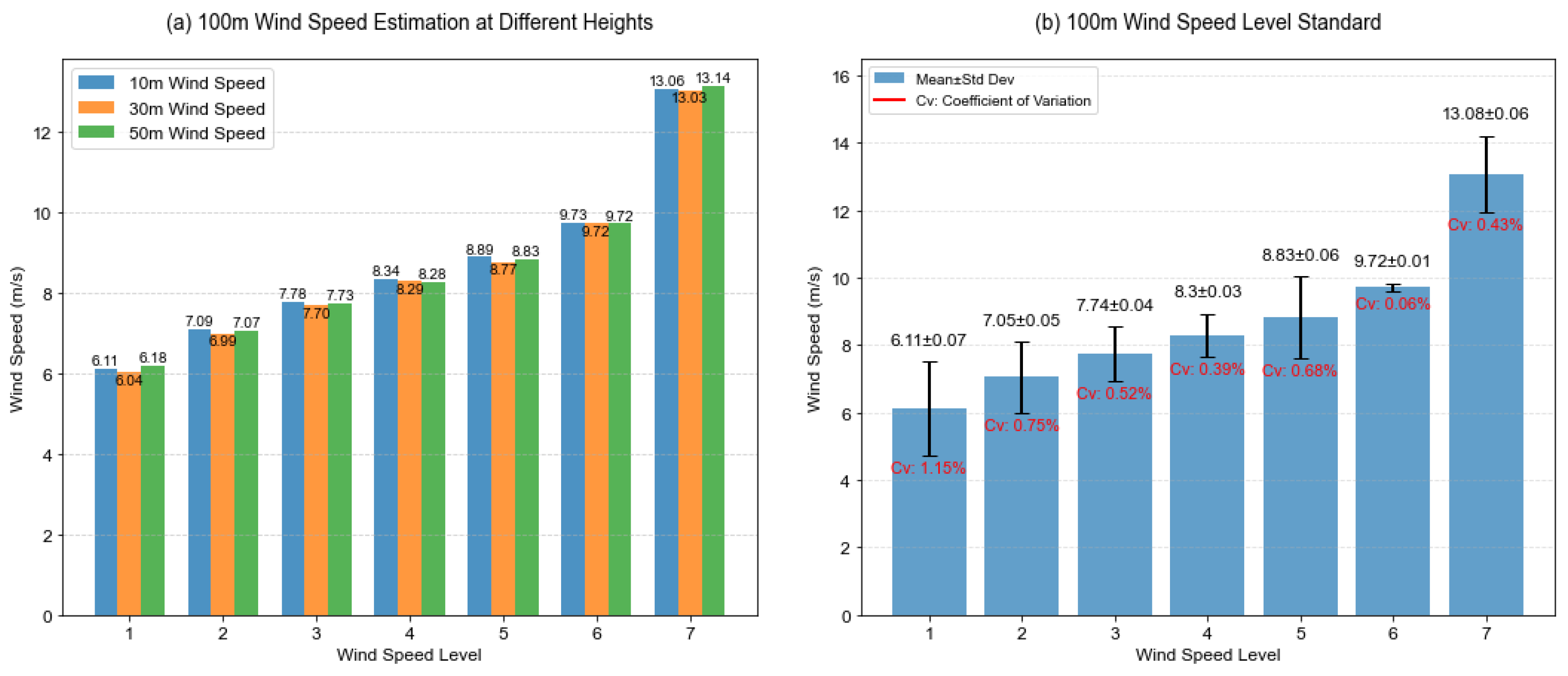
Following the WPD classification criteria of the Wind Energy Resource Assessment Method for Wind Farms (GB/T 18710-2002) and utilizing the wind shear power law (Equation (6)), we derived the wind speed classification thresholds at 100 m height from the current standards for 10 m, 30 m, and 50 m heights. As shown in Figure 1a, the differences in wind speed among these lower heights were negligible (<0.1 m·s⁻¹), indicating that vertical wind speed variations below 100 m have a negligible effect on the classification outcome.

We then consolidated these three sets of thresholds into a single standard for 100 m height by calculating their mean values. The associated uncertainty was quantified by the standard deviation and coefficient of variation (Figure 1b). The results show that both metrics are very low, indicating excellent agreement between the thresholds derived from different reference heights. The derived wind speed ranges for each grade are well-defined and practical for implementation. Therefore, we propose that this classification scheme for 100 m wind speeds be adopted as a meteorological standard.

3. Results and Discussion

3.1. Data Comparison

In recent years, scatterometers used for observing sea surface wind fields include HY-2A, OSCAT, QuikSCAT, and ASCAT, etc. Among these, HY-2A, QuikSCAT, and OSCAT operate in the same Ku-band frequency range and are thus significantly affected by rainfall [30,31,32]. ASCAT operates at a frequency of 5.25 GHz in the C band, making it less susceptible to cloud and rain interference. Scholars both domestically and internationally have conducted relevant assessments and validations of ASCAT scatterometer wind field products, demonstrating that ASCAT wind field products exhibit high accuracy [33,34,35,36].

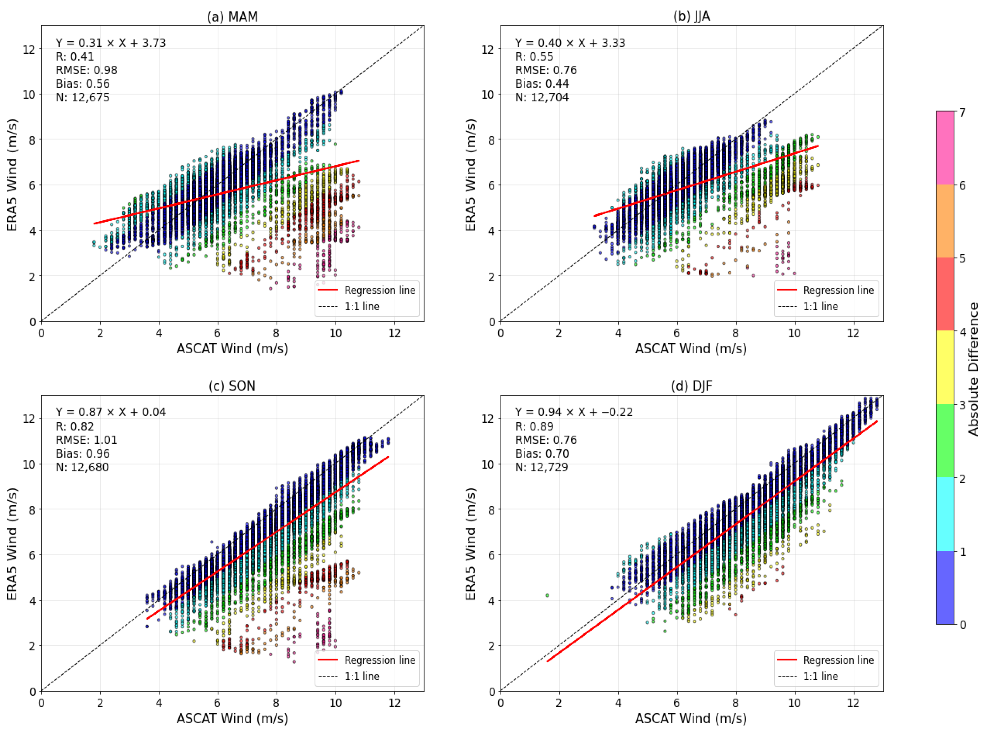
Therefore, we selected ASCAT data for comparative validation against ERA5 data. Figure 2 shows the seasonal discrepancies in wind speed retrievals between ERA5 and ASCAT. To facilitate seasonal comparison, the four seasons are defined as follows: boreal spring (March–May, MAM), boreal summer (June–August, JJA), boreal autumn (September–November, SON), and boreal winter (December–February, DJF). In DJF, the two datasets exhibit remarkable consistency: the regression slope reaches 0.94 (formulated as y = 0.94x − 0.22), accompanied by a high correlation coefficient (R = 0.89) and a negligible bias of 0.7. For SON, while the linear relationship remains robust (slope = 0.87, R = 0.82), a notable bias of 0.96 implies the necessity of bias correction for ERA5 data in this season. In contrast, MAM and JJA demonstrate relatively weaker linear correlations, signifying higher uncertainties. This may be because MAM is a monsoon transition period with highly variable wind directions and speeds, reducing consistency between instantaneous satellite observations and reanalysis data. Summer coincides with peak tropical cyclone activity, where satellite-retrieved winds show significant biases under high-wind conditions—especially for speeds >10 m·s⁻¹, where over 90% of retrievals are underestimated. Additionally, increased summer rainfall can interfere with scatterometer measurements, and the fundamental difference in temporal sampling (instantaneous ASCAT overpasses versus hourly averaged ERA5 outputs) further amplifies discrepancies during periods of high wind variability. These combined factors explain the lower correlation in spring and summer [27,33,37,38,39]. In summary, the substantial annual and seasonal agreement, especially in autumn and winter, validates ERA5 as a feasible alternative to ASCAT for subsequent wind resource assessments. This finding highlights the utility of ERA5 for long-term wind energy studies in the northern SCS, provided that its seasonal limitations are explicitly considered.

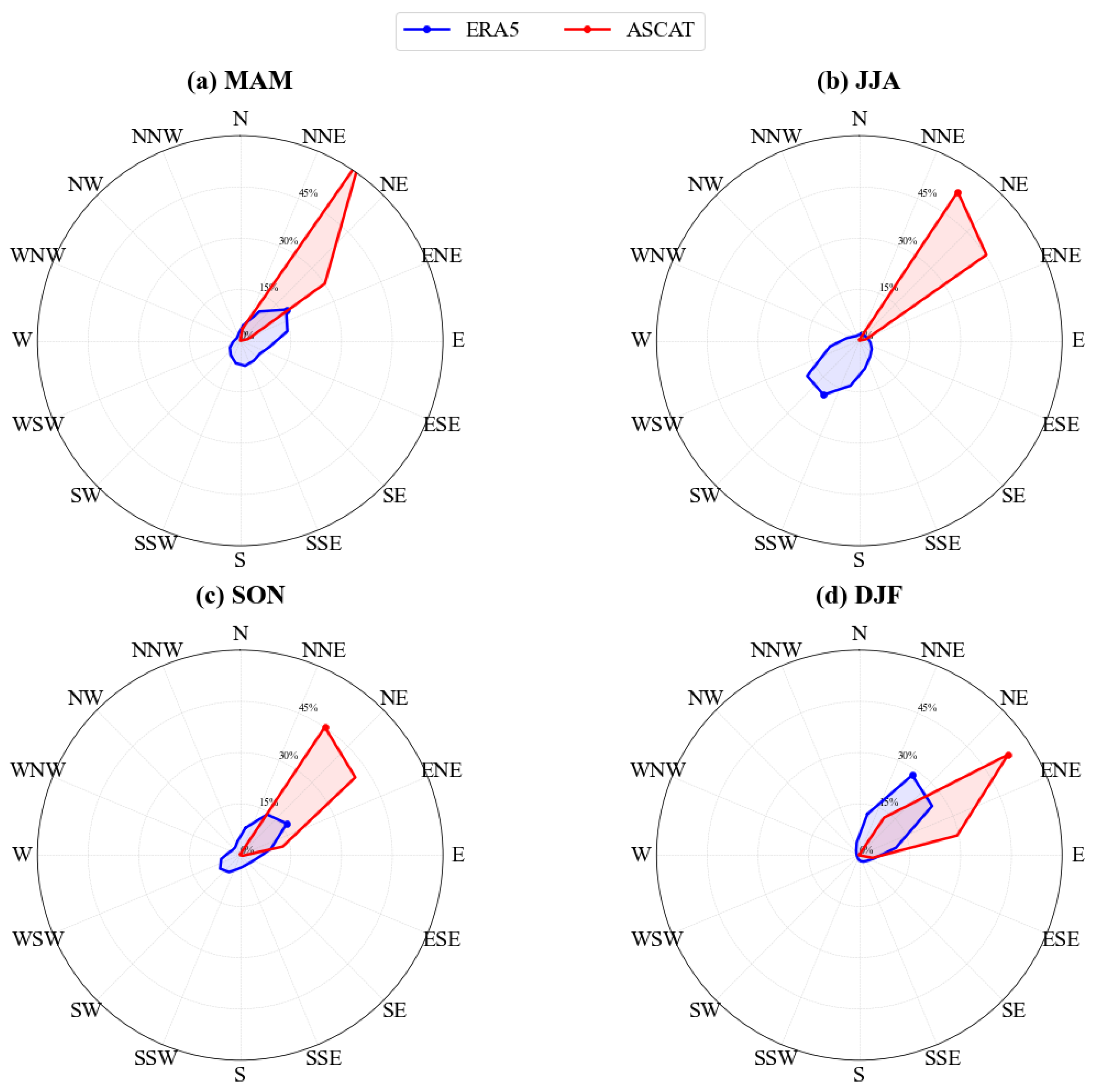
The seasonal wind direction patterns derived from ERA5 and ASCAT exhibit both consistencies and notable discrepancies. It is shown in Figure 3 that in DJF, ERA5 shows a dominant north-northeasterly (NNE) wind direction (28.13%, mean direction 81.2°), while ASCAT indicates a dominant northeasterly (NE) wind direction (52.92%, mean direction 60.8°). Both datasets capture the prevailing northeasterly monsoon, with ASCAT showing a more concentrated directional distribution. In JJA, ERA5 records a dominant south–south westerly (SSW) wind (19.06%, mean direction 197.2°), consistent with the summer monsoon pattern, whereas ASCAT continues to show a dominant north–northeasterly (NNE) wind (52.40%, mean direction 44.1°), likely due to the limited temporal coverage and different sampling characteristics of satellite scatterometer data. Despite these differences, the ERA5 data more effectively capture the seasonal reversal of monsoon winds, making it more suitable for long-term wind energy assessment in the northern SCS.

3.2. Spatial Comparison of Wind Field Datasets

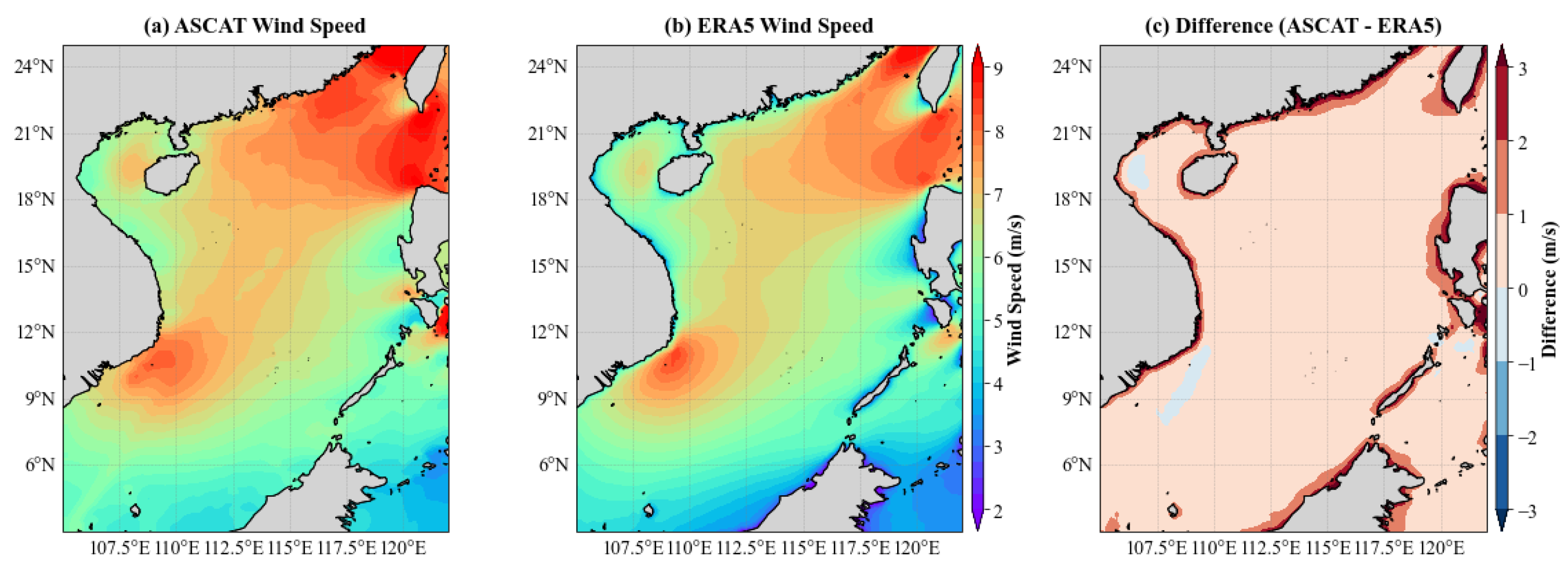
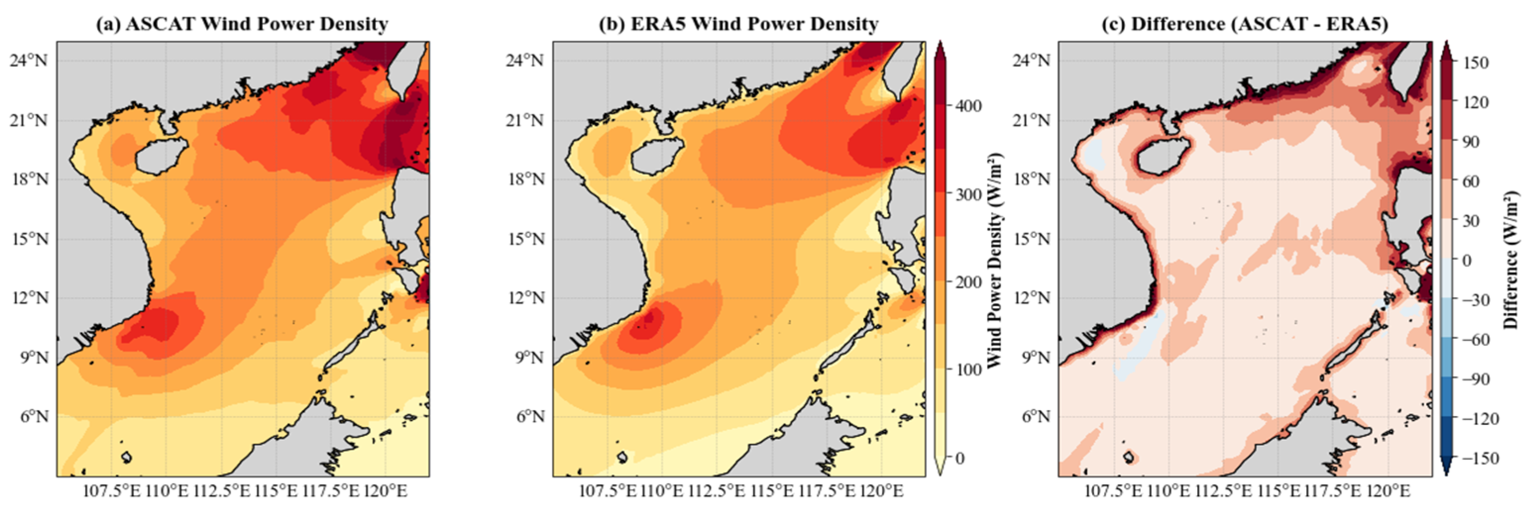
To further demonstrate the consistency between the two datasets, Figure 4 and Figure 5 present the spatial comparison of annual mean wind speed and wind power density between ASCAT and ERA5. For both variables, the spatial distributions exhibit a pronounced northwest-to-southeast gradient. High wind speeds (7–8 m·s⁻¹) and high WPD values (300 W·m⁻²) are concentrated southwest of Taiwan and southeast of Vietnam, reaching maximum values of up to 9 m·s⁻¹ and 400 W·m⁻², respectively, in these hotspot regions. Overall, ASCAT values are slightly higher than ERA5 across most of the study area, with positive biases generally ranging from 0 to 1 m·s⁻¹ for wind speed and from 30 to 120 W·m⁻² for WPD.

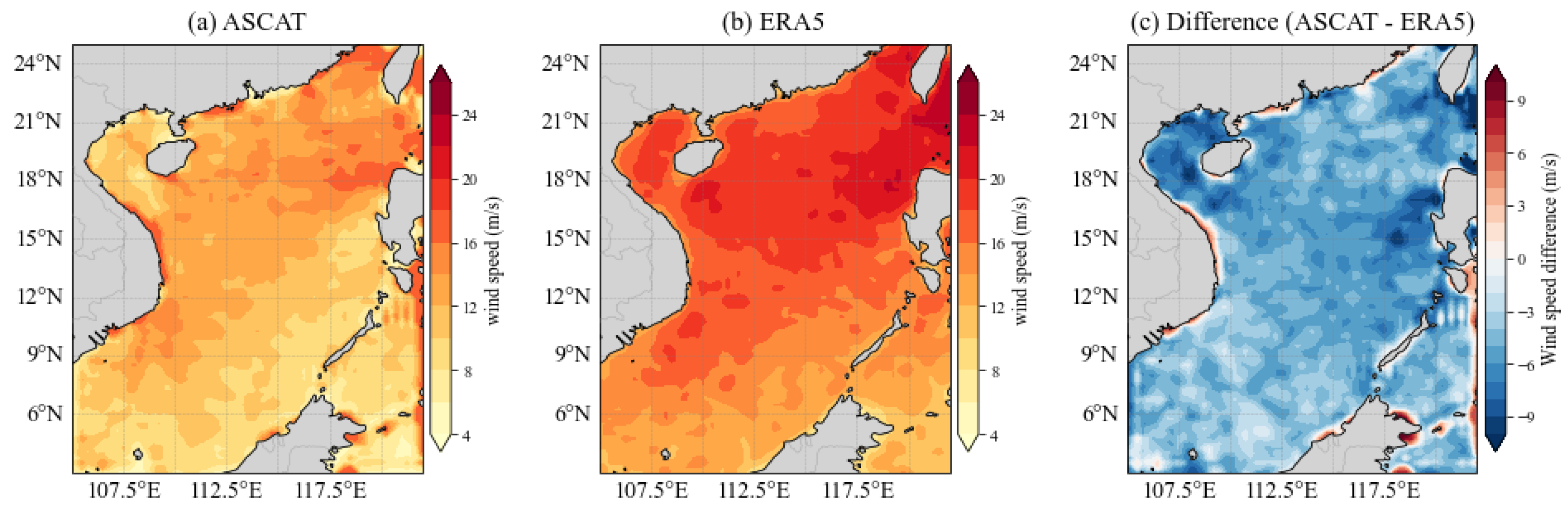
Figure 6 follows the extreme wind assessment methodology outlined in IEC 61400-1:2019 (Section 6.3.3.2) [40]; we calculated the 50-year return period wind speed by fitting the Gumbel distribution to the annual maximum wind speed time series at each grid point [29]. The 50-year return period wind speeds derived from ASCAT are generally lower than those from ERA5 across most of the study area. This discrepancy is likely attributable to the limited temporal coverage of ASCAT observations, which may not fully capture the full range of extreme wind events, particularly those associated with tropical cyclones. In contrast, ERA5 is a reanalysis product that assimilates a wide range of observational data, including satellite measurements and in situ observations from around the world, over an extended historical period. This long-term record enables ERA5 to better represent the climatological characteristics of extreme wind events, including those associated with typhoons [27,38,39]. Consequently, ERA5 provides a more comprehensive characterization of extreme wind conditions.

3.3. Comprehensive Analysis of Wind Energy Resources

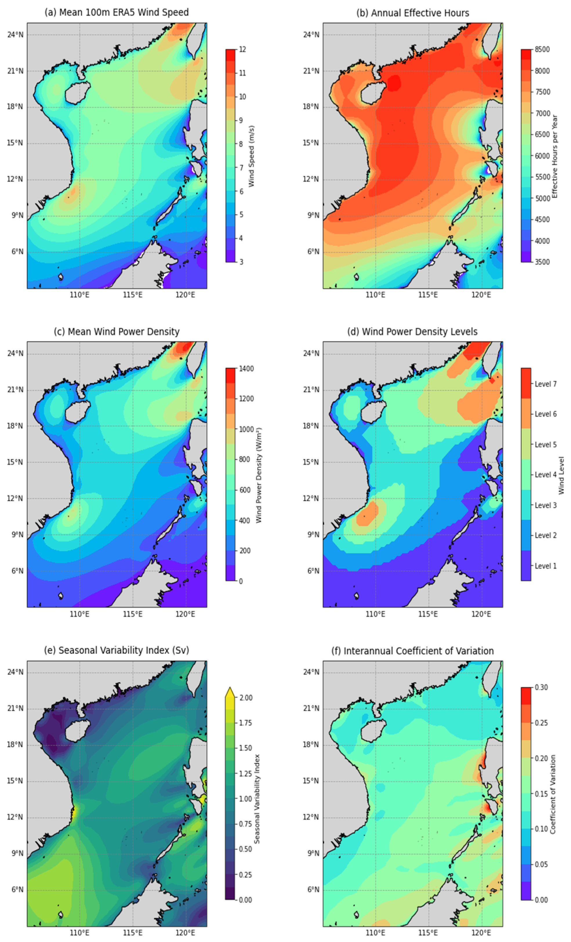
To analyze the long-term characteristics of wind energy potential in the SCS, Figure 7 presents a comprehensive analysis, including (a) annual mean wind speed, (b) annual wind availability, (c) annual mean wind power density, (d) wind energy classification, (e) seasonality index, and (f) interannual coefficient of variation.

Figure 7a illustrates the spatial distribution of the long-term mean wind speed at 100 m, which exhibits a pronounced northwest-to-southeast gradient, with wind speeds decreasing towards the southeastern basin. The southeastern basin is characterized by mean speeds below 7.0 m·s⁻¹, while higher speeds (≥10.0 m·s⁻¹) are predominantly located southwest of Taiwan and southeast of Vietnam. Intermediate wind speeds (5.0–10.0 m·s⁻¹) are observed in coastal regions, including the Beibu Gulf, around Hainan Island, and in the central basin.

For wind energy potential analysis, we calculated the annual wind availability (Figure 7b), defined as the count of hours per year when the 100 m wind speed is within the effective operating range (3–25 m·s⁻¹). Wind availability in most of the region exceeds 6457 h per year on average, with maximum availability reaching up to 8283 h per year in the most favorable locations, particularly southwest of Taiwan, southeast of the Pearl River Delta, and southeast of Vietnam.

The mean wind power density (Figure 7c) exhibits a spatial pattern consistent with that of mean wind speed, showing a strong meridional gradient with higher values in the north. Large WPD areas (≥1000 W·m⁻²) are concentrated in the Taiwan Strait and southeast of Vietnam, while the southeastern basin is characterized by low WPD (<300 W·m⁻²). Based on the classification criteria from the Chinese national standard GB/T 18710-2002, the wind energy resources are classified in Figure 7d. The southeastern basin is predominantly classified as Marginal or Poor (below Class 3), whereas Good to Excellent resources (Class 3 and above) dominate the northwestern waters. Notably, Outstanding to Superb resources (up to Class 7) are found southwest of the Taiwan Strait and southeast of Vietnam.

The seasonality index (Figure 7e) reveals significant spatial heterogeneity. Most of the basin experiences high seasonal variability (index = 0.75–1.5), while the Beibu Gulf and areas southeast of the Pearl River Delta show exceptional seasonal stability (index ≈ 0.25). The interannual coefficient of variation in annual mean WPD (Figure 7f) ranges from 0 to 0.3 across most of the basin, with relatively low values (0–0.1) in the northern regions and relatively high values (0.1–0.3) in the central and southeastern basins [12].

In summary, the wind resources of the northern SCS are characterized by high abundance and high stability, both seasonally and interannually. This combination identifies the northern regions as the most reliable and promising areas for offshore wind development.

3.4. Effective Wind Energy Reserve (EWER)

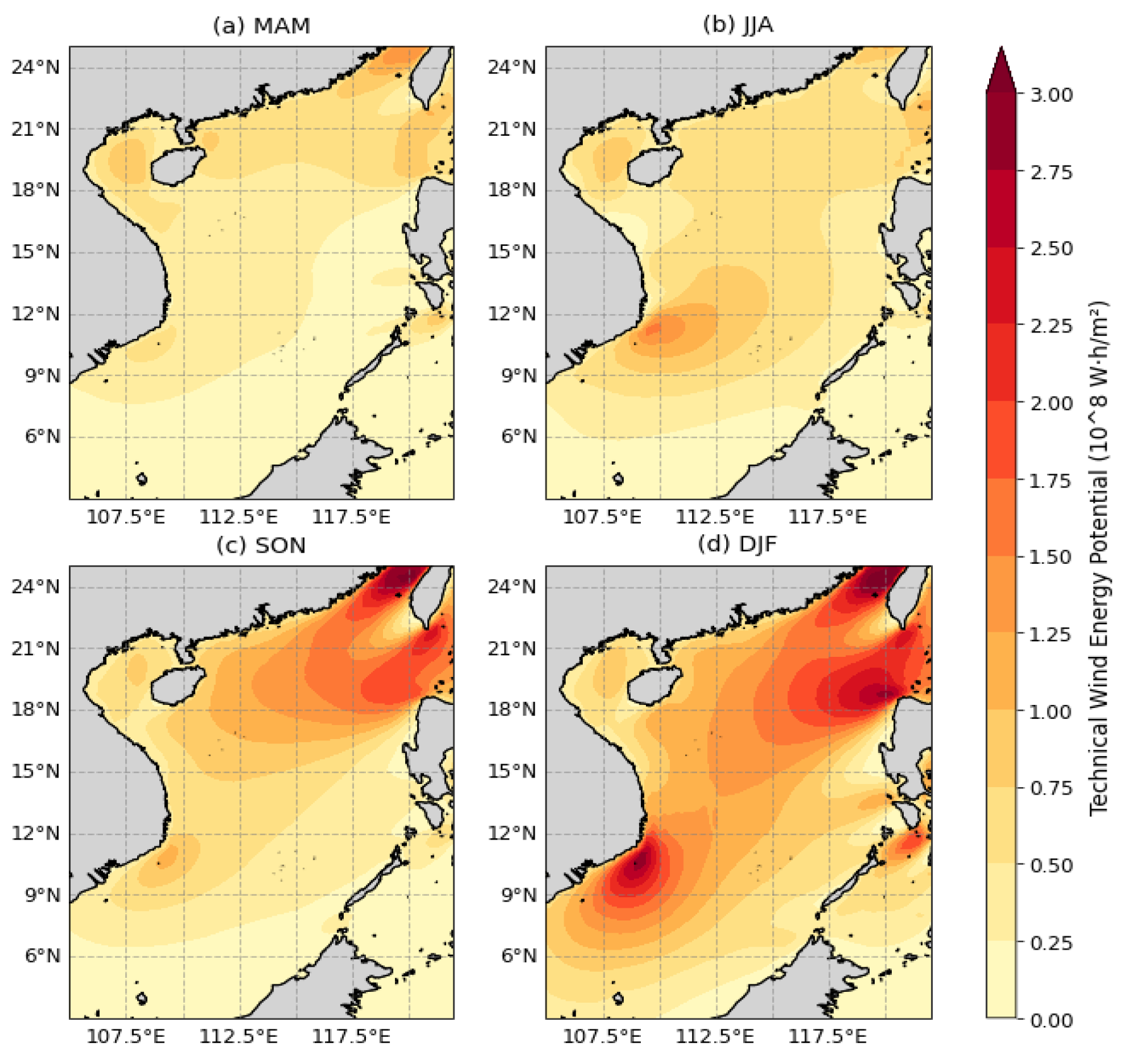
As shown in Figure 8, seasonal EWER reveals strong variations in magnitude in different seasons. The EWER reaches its peak in winter (up to 2.4 × 10⁸ Wh·m⁻² in optimal zones), followed by autumn, and drops to the valley in spring. The Taiwan Strait and eastern sea of Vietnam maintain superior potential across all seasons, with performance being particularly enhanced during autumn and winter due to intensified monsoon winds.

3.5. Capacity Factor (CF)

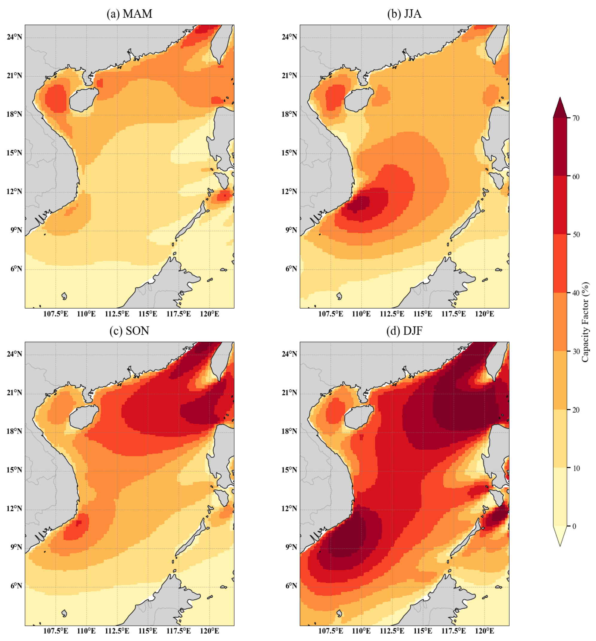
As shown in Figure 9, the seasonal CF exhibits a spatial distribution consistent with that of WPD and wind speed. High CF values are concentrated in the resource-rich hotspots southwest of Taiwan and southeast of Vietnam, where values generally exceed 30% across all seasons. Winter achieves the highest CF, with most areas in these hotspots exceeding 50%, reflecting the strongest monsoon winds during this season [28]. Summer shows the lowest CF, while spring and autumn exhibit intermediate values. The Taiwan Strait and the eastern sea of Vietnam maintain a superior CF throughout the year, with particularly enhanced performance during autumn and winter due to intensified monsoon winds. These results indicate that the northern SCS, especially the regions southwest of Taiwan and southeast of Vietnam, possesses substantial potential for efficient wind power generation.

3.6. Leading Modes of Wintertime WPD

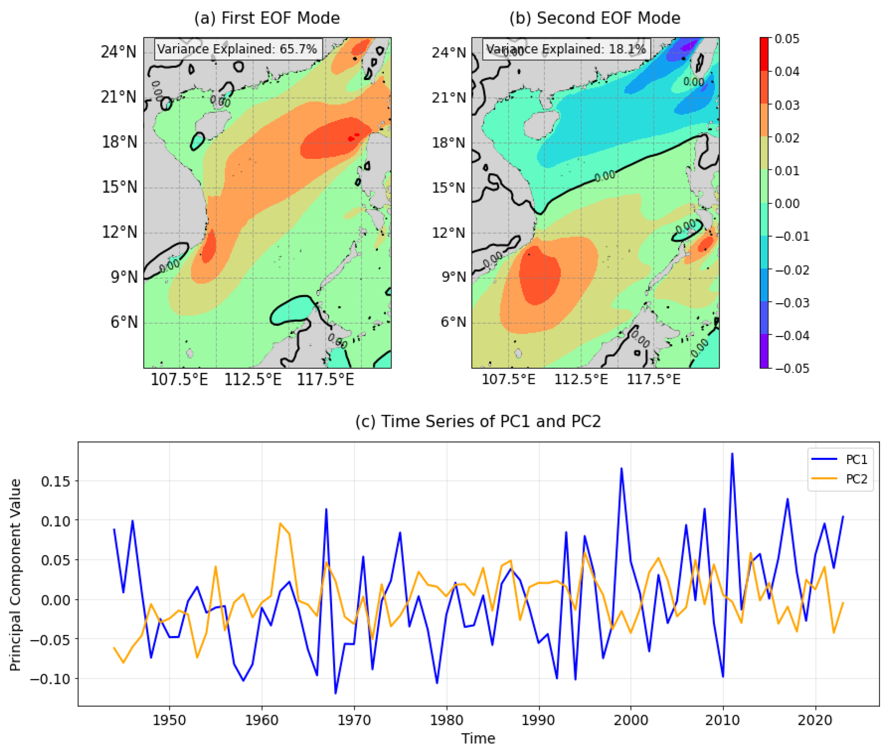
To extract the leading mode of wintertime (December–February) WPD over the SCS, an empirical orthogonal function (EOF) analysis is conducted [41]. As shown in Figure 10, the first EOF mode shows a spatially uniform WPD anomaly in the SCS, with prominent interannual–interdecadal variability and an increasing trend after the 1990s (PC1), which accounts for 65.7% of the total variance. Therefore, this mode can be considered as a homogenous mode, suggesting that winter WPD over most of the SCS presents coherent year-to-year variability. The second mode (PC2) presents a meridional dipole structure (north–south contrast) of the WPD anomaly, accounting for additional 18.1% (Figure 10b). In order to represent the primary information of WPD’s long-term variability, the normalized PC1 time series (Figure 10c) is defined as an indicator for the variability of WPD over the SCS and used in the following discussion.

3.7. Characteristics of Principal Component of Winter WPD

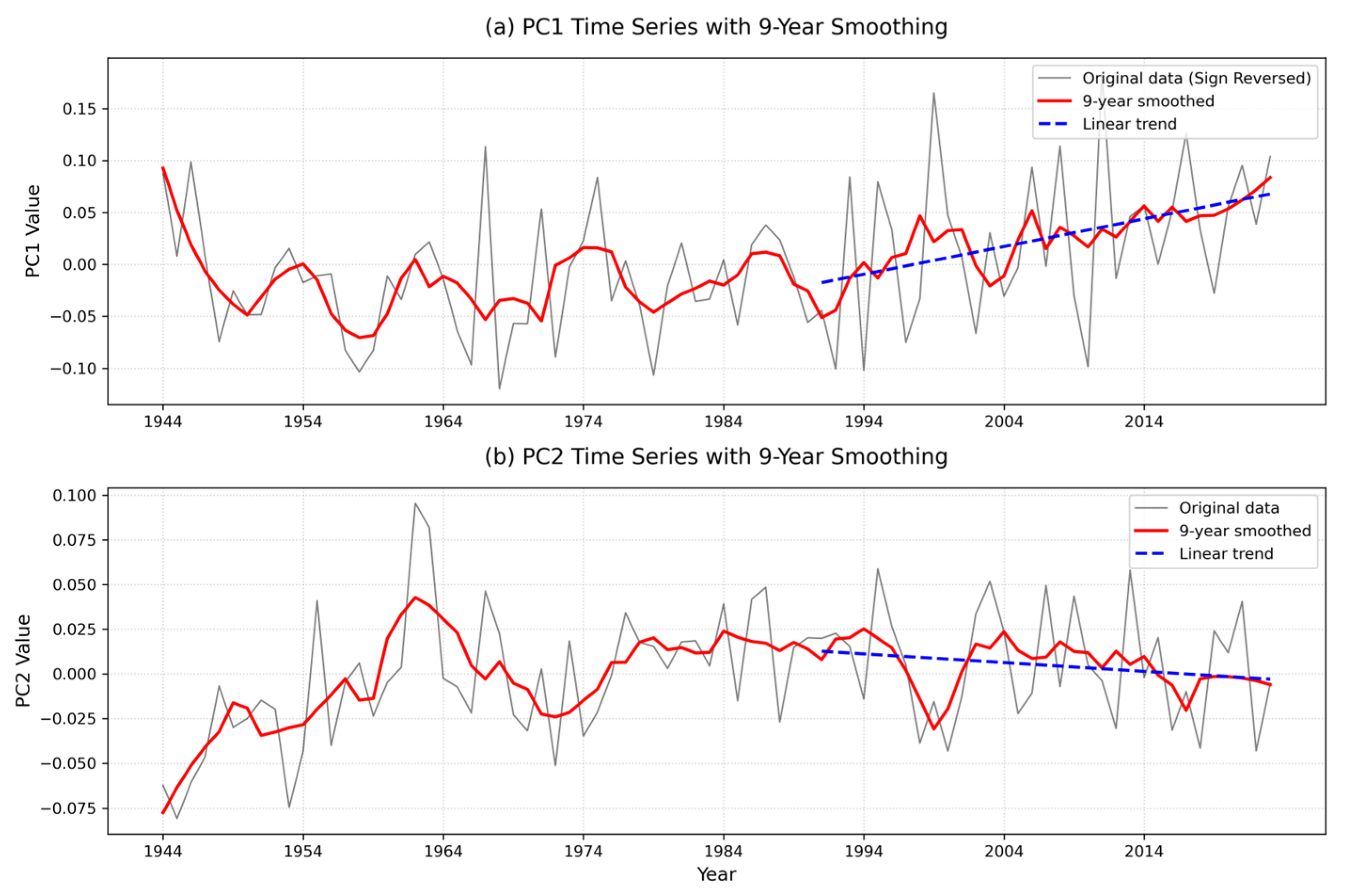
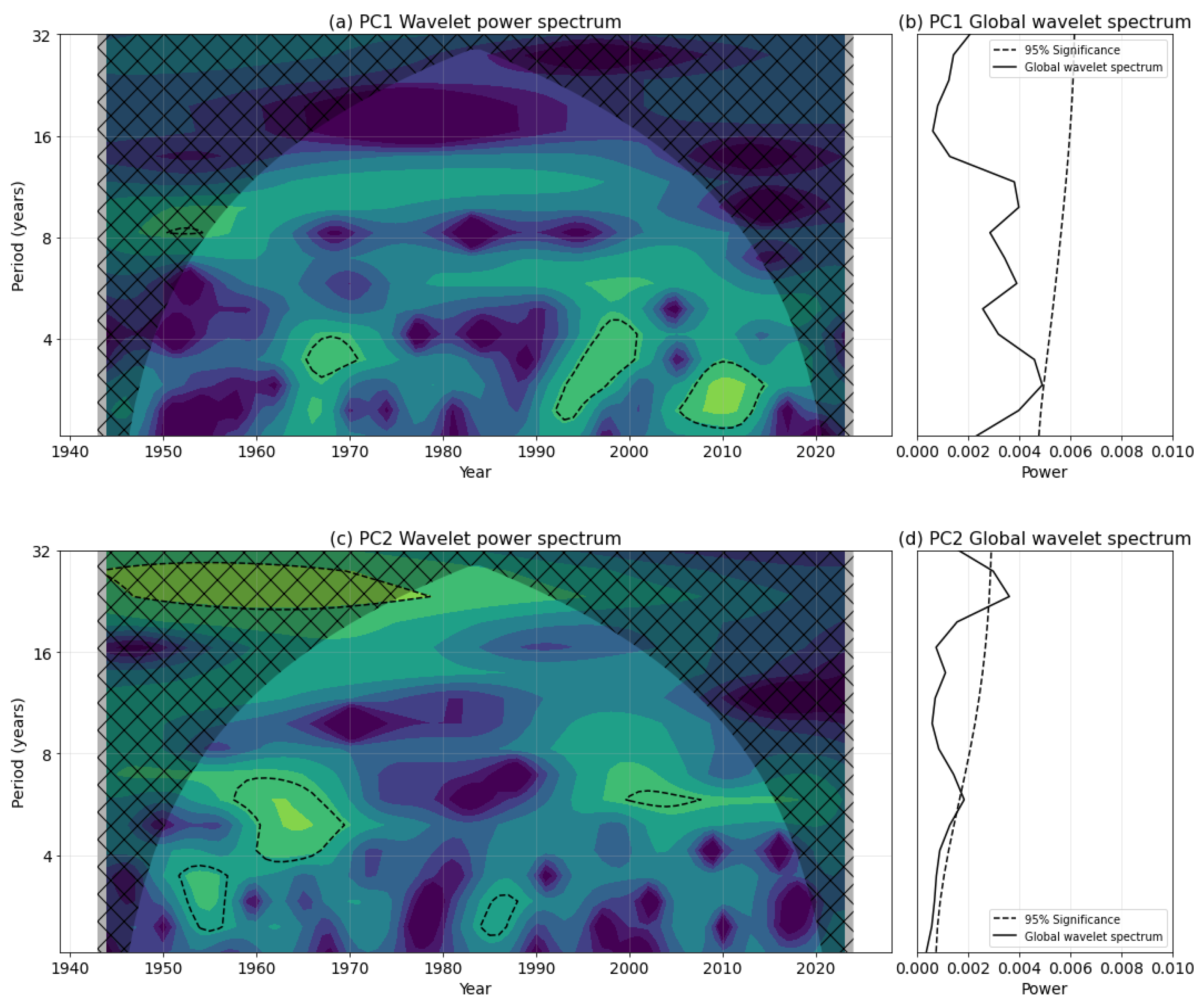
The time series of PC1 shows strong interannual–interdecadal variability with a significant increasing trend in the last three decades. A 9-year moving average reinforces this interdecadal variability and a highly significant (p < 10⁻⁶) increasing trend from 1991 to 2023 (Figure 11a). The wavelet power spectrum presents significant interannual variability (exceeding the 95% confidence level against red noise) at periods of 2–4 years. This band of variability manifested as two active epochs: 1992–2001 and 2005–2014. The global wavelet spectrum confirms that this 2–4-year oscillation is an intrinsic mode of variability persisting throughout the 1944–2023 record (Figure 12a,b).

Analysis of the secondary mode (PC2) reveals distinctly different characteristics. The 9-year smoothed PC2 shows a statistically significant but climatically modest declining trend (p = 0.043; slope = −0.009 W·m⁻²·decade) post-1991 (Figure 10b). The linear model explains very little variance (R² = 0.126) and has wide prediction intervals (±0.025), indicating that this trend is weak and likely part of the background low-frequency variability rather than a robust climatic signal. PC2 identifies significant oscillations in the 4–6 year band, with active phases occurring in 1957–1969 and 1999–2007. Given its different temporal characteristics from PC1, the variability in PC2 is likely modulated by a different set of drivers, potentially involving other facets of Pacific decadal variability or remote forcing mechanisms that affect the meridional dipole pattern.

3.8. Impact of Extratropical Sea Surface Temperature on Winter WPD in the SCS

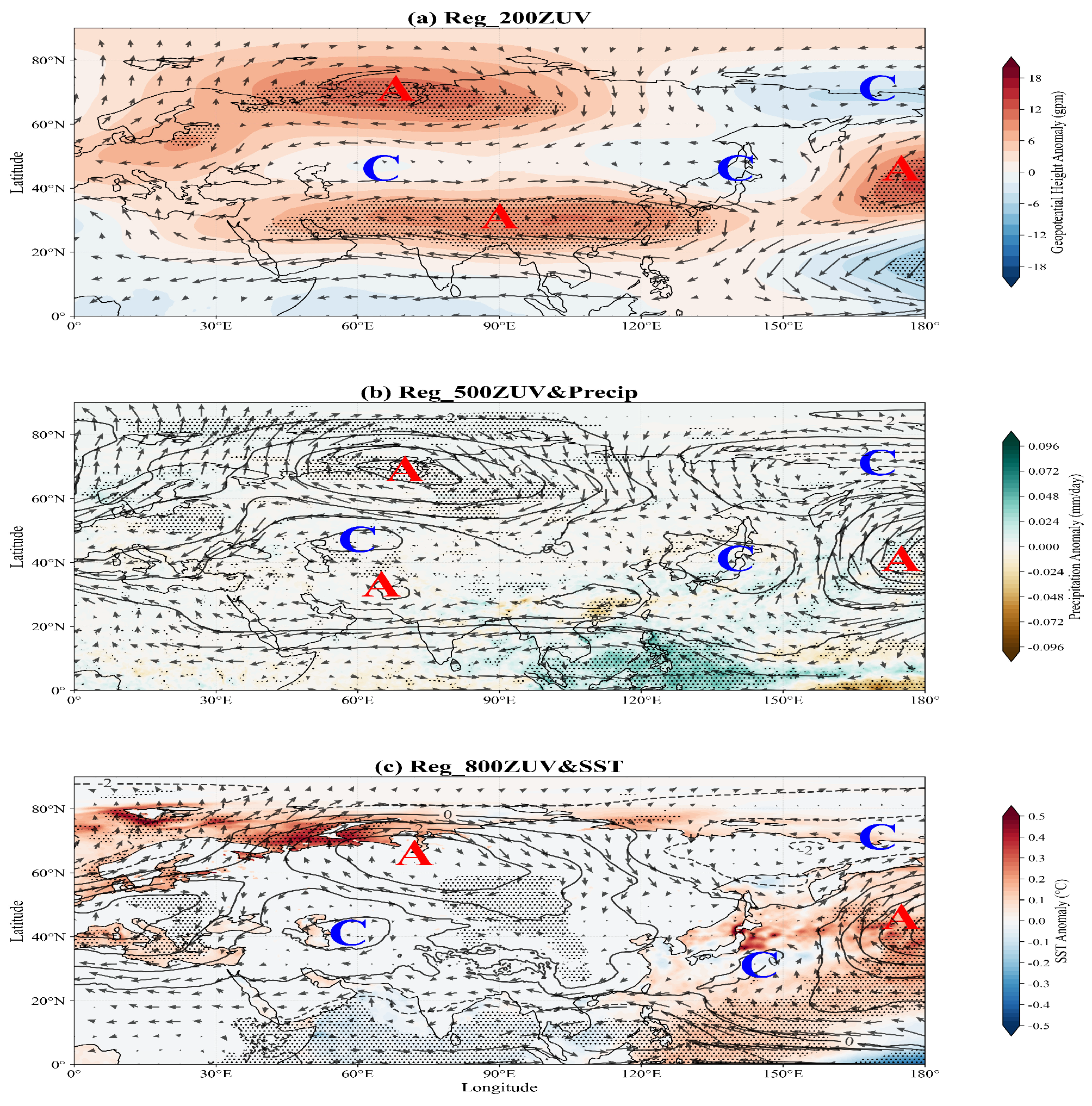
To reveal the dynamic mechanisms underlying the intensification of the winter monsoon in the SCS, this section analyzes atmospheric circulation anomalies from the upper (200 hPa), middle (500 hPa), to lower (800 hPa) troposphere. The analysis demonstrates that the intensification of the SCS winter monsoon is a systematic process involving vertical coupling among polar sea surface temperature (SST) anomalies and the upper-level steering, mid-level transmission, and lower-level response. Regression ofPC1 onto anomalous SST, geopotential height and wind fields reveals that the intensification of the SCS winter monsoon is closely associated with anomalous warming in the Barents Sea. The warming SST heats the overlying atmosphere, generating a quasi-barotropic anticyclonic circulation anomaly aloft (Figure 13). This disturbance propagates from high to low latitudes via quasi-stationary Rossby waves, which is similar to the results in Tan et al. (2023) [42].

At 200 hPa, positive geopotential height anomalies are observed over the mid-high latitudes of Eurasia (60° E–120° E, 40° N–80° N) and the eastern North Pacific (180° E, 40° N–60° N), while negative anomalies occur along the East Asian coast (120° E–150° E, 40° N–60° N), forming a wave train structure of “anticyclone–cyclone–anticyclone” (Figure 13a). At 500 hPa, the circulation is highly coupled with that at 200 hPa: the positive height anomaly over Eurasia persists, corresponding to a strengthened and downward-extended blocking high; the negative anomaly along the East Asian coast deepens, forming a strong East Asian trough (Figure 13b). The wind field exhibits a pronounced northerly anomaly over the mid-high latitudes of East Asia, accompanied by significant positive precipitation anomalies over the SCS and the tropical western Pacific. The positive precipitation anomalies indicate the release of large-scale latent heat of condensation, heating the atmosphere and thus favoring the formation of cyclonic circulations east of the South China Sea and the Philippine Sea (Figure 14a and Figure 15a). At 800 hPa, the positive height anomaly over the mid-high latitudes corresponds to an enhanced Mongolian cold high, while the negative anomaly along the East Asian coast corresponds to a lower-level low-pressure system or cyclone, leading to a substantially increased sea–land pressure gradient. A pronounced northeasterly wind anomaly appears over the SCS, along with positive SST anomalies over the SCS and the tropical western Pacific (Figure 13c).

3.9. Impact of Tropical SST Anomaly on WPD over the SCS

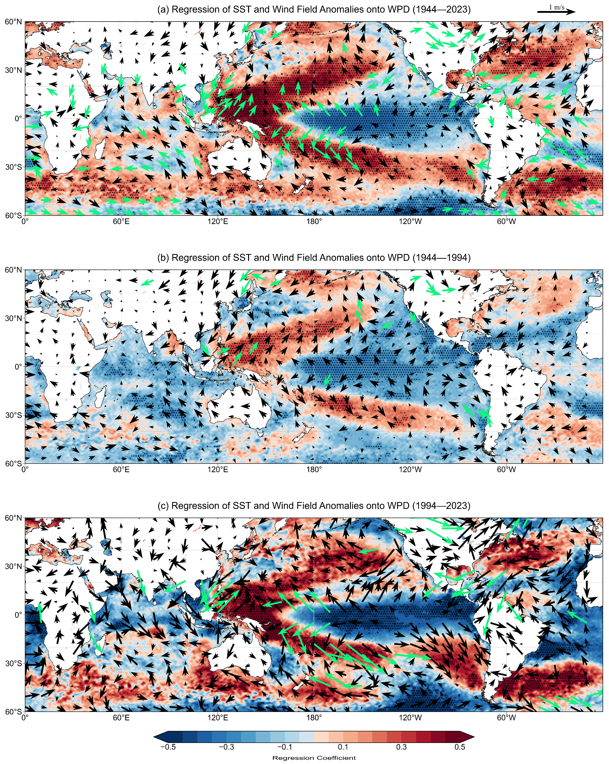
In this section, our study focuses on PC1, because the first EOF mode of WPD in the SCS accounts for 65.7% of the total variance, explaining primary signals of WPD variability. For the homogenous mode of WPD in the SCS, the regression of the SST field (Figure 14a) onto PC1 presents significant K-shaped warming in the western Pacific and triangular cooling with prominent negative anomalies in the tropical central and eastern Pacific. This spatial pattern is analogous to the “Mega-ENSO” mode proposed by [43], which is an intrinsic interdecadal variabilities. Anomalous warming in the warm pool region drives enhanced convective motion, favoring the formation of cyclonic circulation anomalies in the SCS and east of the Philippine Sea, which in turn strengthens the northerly wind over the SCS (Figure 15a).

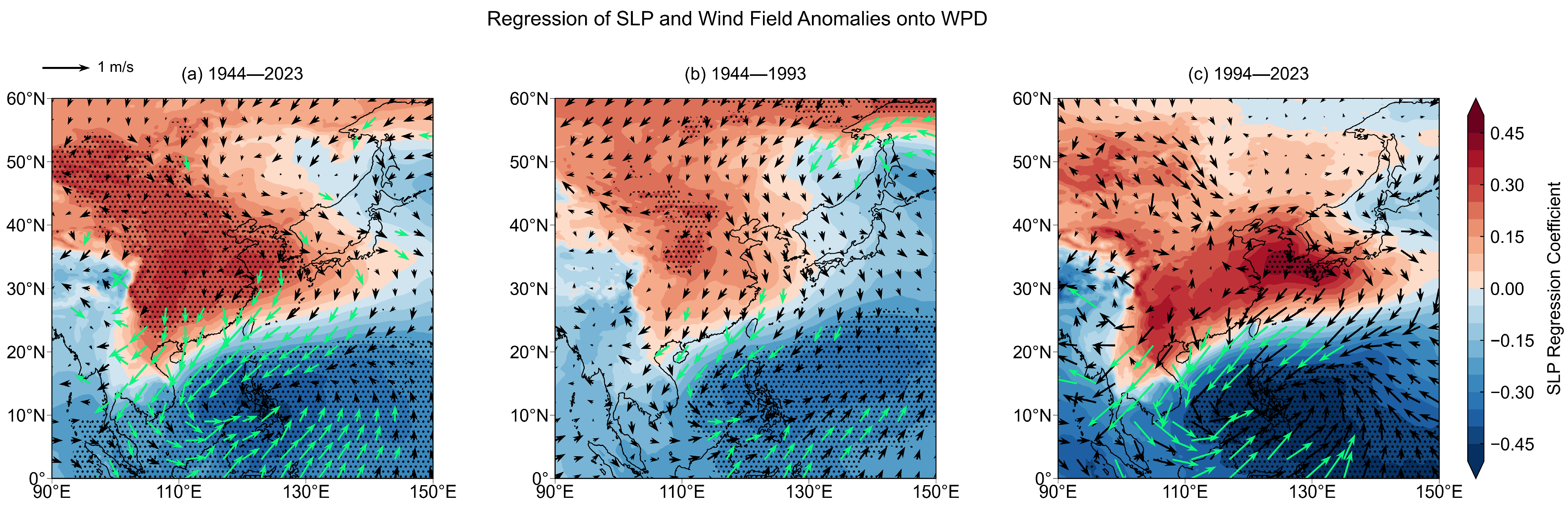
As shown in Figure 14b,c, a comparison of oceanic and atmospheric anomalies before and after the significant increase in WPD (the 1990s) reveals that the Mega-La Niña signal has strengthened significantly since the 1990s, implying a marked increase in both the frequency and intensity of Mega-La Niña events after 1990. In addition, SST anomaly signals in the southern Indian Ocean and North Atlantic have also intensified (Figure 14c). Correspondingly, an anomalous low pressure over the SCS and Philippine Sea and anomalous high pressure over East Asia have both intensified since the 1990s. The stronger pressure gradient between them enhances northerly wind anomalies in the central and northern SCS (Figure 15b,c).

Therefore, Mega-ENSO can be considered as an important forcing factor in the multidecadal variability of WPD in the SCS, which is instructive for understanding the variability of wind energy in the SCS and for future physically constrained predictions.

3.10. Integrated Discussion

The strong agreement between ASCAT and ERA5 in autumn and winter confirms the reliability of ERA5 for wind energy analysis over the SCS. This is consistent with previous validation studies. Gao et al. [37] reported correlation coefficients of 0.62–0.77 for wind speed between satellite products and buoys, with mean biases of 0.46–0.50 m·s⁻¹. Zhang [10] further validated ERA5 against coastal stations, achieving a correlation of 0.91, though biases were slightly higher in coastal areas due to complex topography. The slight underestimation of high-frequency variability during extreme events aligns with Li et al. [44], who found ASCAT winds to be systematically lower than QuikSCAT at high wind speeds (>15 m·s⁻¹), with biases up to 1.5 m·s⁻¹ in the Taiwan Strait. These results collectively confirm that both ASCAT and ERA5 provide reliable wind fields for long-term resource analysis in the SCS, though caution is needed when analyzing extreme wind conditions [45].

The pronounced northwest-to-southeast gradient in wind speed and WPD reflects the dominant influence of the East Asian monsoon system [46]. The high-wind hotspots identified in our study—southwest of Taiwan and southeast of Vietnam—correspond to regions where topographic effects accelerate monsoon flows [47]. Gale events in the SCS occur most frequently in winter, followed by autumn, consistent with the seasonal energy distribution observed in our WPD analysis [45]. The spatial pattern of wind resources also reflects the influence of Kuroshio intrusion on local wind fields through air–sea interactions [46]. The high stability of wind resources in the northern SCS (interannual C_V = 0–0.3; seasonal C_V < 0.4) aligns with previous characterizations. The Beibu Gulf exhibits particularly stable conditions due to its semi-enclosed geometry and reduced typhoon exposure [45]. The Beibu Gulf and areas southeast of the Pearl River Delta show exceptionally low seasonal variability (seasonality index ≈ 0.25) [10]. Conversely, the high variability southwest of the Philippines (C_V > 0.4, reaching 0.9 in spring) reflects the influence of tropical cyclone activity, with over 50% of summer and autumn gale events associated with tropical cyclones [45].

Interannual variability in the northern SCS is modulated by large-scale climate modes, with the first EOF mode capturing basin-wide wind intensity and exhibiting 3–4 year periodicity correlated with ENSO. The EOF analysis of winter WPD reveals that the first mode accounts for 65.7% of the total variance, with predominantly positive loadings across the region, indicating coherent basin-scale variability. The significant increasing trend in PC1 since approximately 1990 suggests a notable enhancement of winter wind resources in recent decades. Wavelet analysis identifies significant 2–6-year oscillations matching ENSO’s periodicity, providing strong temporal evidence for ENSO’s role in regulating interannual wind resource variability. The mechanism linking ENSO to SCS wind variability involves the Philippine Sea anticyclone/cyclone anomaly, with ENSO accounting for approximately 17.5% of interannual variance [20,48]. In addition, other climate modes such as the Pacific Decadal Oscillation (PDO), North Atlantic Oscillation (NAO), and Southern Annular Mode (SAM) also modulate wind variability on longer timescales through atmospheric teleconnections. This air–sea coupling mechanism explains why La Niña conditions enhance Philippine Sea cyclonic circulation, generating northeasterly anomalies that constructively reinforce the East Asian winter monsoon and increase WPD in the northern SCS [21,22,23,24].

The findings of this study have important implications for offshore wind energy development in the SCS. The identification of stable, resource-rich areas—particularly southwest of Taiwan and southeast of Vietnam—provides clear guidance for wind farm siting, while the strong seasonal variability suggests that energy storage may be necessary for year-round reliability [7,49,50]. ENSO-driven interannual variability underscores the need to consider climate variability in long-term planning. Substantial development potential exists despite ongoing climate change [51,52]. Deng et al. [29,53,54] demonstrated that greenhouse gas forcing plays a dominant role in enhancing wind resources, supporting the viability of long-term wind energy development in the region. Limitations include uncertainties in representing extreme events and complex coastal dynamics, as well as inter-satellite discrepancies at high wind speeds. Future research should prioritize higher-resolution downscaling, integration with marine spatial planning, and the investigation of multi-scale climate mode interactions [38,39,55].

4. Conclusions

Based on an analysis of high-resolution ERA5 100 m wind data, this study provides a comprehensive assessment of the wind energy resources in the northern SCS. The main conclusions are as follows:

1. ASCAT and ERA5 show strong agreement in winter (R = 0.89) and autumn (R = 0.82). Both datasets capture a northwest-to-southeast gradient, with wind speeds ≥10 m·s⁻¹ and WPD ≥ 900 W·m⁻² concentrated southwest of Taiwan and southeast of Vietnam. ASCAT wind speeds and WPDs are slightly higher than ERA5 across most of the basin. The 50-year return period wind speeds from ERA5 are higher than those from ASCAT.

2. Annual wind availability exceeds 6457 h across most regions, reaching up to 8283 h in optimal locations. The C_V for annual WPD ranges from 0 to 0.3, with northern areas exhibiting the highest stability (C_V = 0–0.1). The seasonality index ranges from 0.75 to 1.5 over most of the basin, with notably lower values (≈0.25) in the Beibu Gulf and areas southeast of the Pearl River Delta.

3. WPD and capacity factor peak in winter (up to 2.4 × 10⁸ Wh·m⁻² and >50%, respectively) and reach minimum values in spring. The Taiwan Strait and eastern sea of Vietnam maintain higher values across all seasons, with peak values in autumn and winter.

4. The first EOF mode of winter WPD accounts for 65.7% of the total variance, with positive loadings across the region. The corresponding principal component has shown an increasing trend since approximately 1990. Wavelet analysis identifies significant 2–6-year oscillations. The interannual variation in winter WPD is associated with SST anomalies in the tropical Pacific and the Arctic Barents Sea. In years with strong wind anomalies in the SCS, mega-La Niña-type SST patterns occur in the tropical Pacific, and warm SST anomalies occur in the Arctic Barents Sea. The 2–6-year oscillations match ENSO periodicity.

Overall, the northern SCS is characterized by abundant wind resources, high seasonal and interannual stability, and substantial technical potential. The resource-rich hotspots (southwest of Taiwan and southeast of Vietnam) demonstrate capacity factors exceeding 50% in winter, indicating excellent suitability for offshore wind farm development. These findings provide a scientific basis for wind farm siting, turbine selection, and long-term operational planning in the region.

References

1. Chen, X.X.; Tian, Y.X. Development trend, advantage potential and orientation choice of China’s new energy industry. Reform 2024, 5, 112–123. (In Chinese) [Google Scholar]
2. Li, X.M.; Liu, S.Z.; Xue, D. Study on the impact of renewable energy development on carbon emissions. Soft Sci. 2024, 38, 86–92+100. (In Chinese) [Google Scholar] [CrossRef]
3. Global Wind Energy Council. Global Offshore Wind Report 2024; GWEC: Brussels, Belgium, 2024. [Google Scholar]
4. State Council of the People’s Republic of China. Notice on Issuing the National Land Planning Outline (2016–2030). 2017. Available online: https://www.gov.cn/gongbao/content/2017/content_5171326.htm (accessed on 10 July 2024). (In Chinese)
5. Heading into Deep Sea and Accelerating Rural Adoption: Wind Power Unlocks New Growth Space. 18 October 2023. Available online: https://baijiahao.baidu.com/s?id=1780059907647149146&wfr=spider&for=pc (accessed on 10 July 2024). (In Chinese)
6. Yang, S.W. Wind Energy Resource Assessment Method Based on Multi-Source Data Fusion. Master’s Thesis, North China Electric Power University, Beijing, China, 2024. (In Chinese) [Google Scholar] [CrossRef]
7. Gao, C.Z.; Zheng, C.W.; Chen, X. Long-term trend analysis of wind energy resources in China’s offshore areas based on CCMP wind field data. Mar. Forecast 2017, 34, 27–35. (In Chinese) [Google Scholar]
8. Xu, Q.; Li, Y.Z.; Cheng, Y.C.; Ye, X.; Zhang, Z. Impacts of climate oscillation on offshore wind resources in China seas. Remote Sens. 2022, 14, 1879. [Google Scholar] [CrossRef]
9. Ding, J.; Wu, G.W.; Chen, J.Q.; Jiang, B. Assessment of ocean wind energy resources in the South China Sea based on CCMP reanalysis wind field data. J. Ocean. Technol. 2022, 41, 83–90. (In Chinese) [Google Scholar]
10. Zhang, J. Long-Term Trends of Sea Surface Wind and Its Impacts on the Marine Environment in the Northern South China Sea Under the Background of Climate Change. Master’s Thesis, South China University of Technology, Guangzhou, China, 2021. (In Chinese) [Google Scholar]
11. Huang, S.C.; Jiang, A.J.; Liu, C.; Chen, B. Reassessment and distribution of wind energy resources in Jiangsu Province. Sci. Meteorol. Sin. 2007, 27, 407–412. (In Chinese) [Google Scholar]
12. Ji, H.F.; Liu, J.T.; Song, X.G.; Ding, Y.Z. Evaluation of wind energy resources in Jiangsu sea area based on ERA5 data. Acta Energiae Solaris Sin. 2023, 44, 320–324. (In Chinese) [Google Scholar]
13. Herbert-Acero, J.F.; Franco-Acevedo, J.R.; Valenzuela-Rendón, M.; Probst-Oleszewski, O. Linear wind farm layout optimization through computational intelligence. In Mexican International Conference on Artificial Intelligence; Springer: Berlin/Heidelberg, Germany, 2009; pp. 692–703. [Google Scholar]
14. Song, Y.L.; Wang, H.; Liu, S.J. Analysis of the impact of hub height variation on investment returns of wind power projects. Appl. Energy Technol. 2018, 12, 51–54. (In Chinese) [Google Scholar]
15. Huang, S.; Cai, Y.F.; Wang, J.; Zhou, C. Applicability of sea surface wind field data in the Yangjiang offshore wind farm area of Guangdong Province. South. Energy Constr. 2024, 11, 111–123. (In Chinese) [Google Scholar] [CrossRef]
16. Chen, K.; Song, M.X.; Zhang, X.; Wang, S. Wind turbine layout optimization with multiple hub height wind turbines using greedy algorithm. Renew. Energy 2016, 96, 676–686. [Google Scholar] [CrossRef]
17. Niang, S.A.A.; Gueye, A.; Drame, M.S.; Ba, A.; Sarr, A.; Nebon, B.; Ndiaye, S.O.; Niang, D.N.; Dioum, A.; Talla, K. Analysis of wind resources in Senegal using 100-meter wind data from ERA5 reanalysis. Sci. Afr. 2024, 26, e02480. [Google Scholar] [CrossRef]
18. Huang, X.L.; Yin, Q.Y.; Mai, Z.T.; Yin, H.N. Characteristics of surface wind field and preliminary exploration of wind energy resources in Yangjiang City in recent 10 years. Guangdong Meteorol. 2016, 38, 53–56. (In Chinese) [Google Scholar]
19. Vasel-Be-Hagh, A.; Archer, C.L. Wind farm hub height optimization. Appl. Energy 2017, 195, 905–921. [Google Scholar] [CrossRef]
20. McPhaden, M.J.; Zebiak, S.E.; Glantz, M.H. ENSO as an integrating concept in Earth science. Science 2006, 314, 1740–1745. [Google Scholar] [CrossRef] [PubMed]
21. Saji, N.H.; Yamagata, T. Structure of SST and surface wind variability during Indian Ocean dipole mode events: COADS observations. J. Clim. 2003, 16, 2735–2751. [Google Scholar] [CrossRef]
22. Marshall, J.; Kushnir, Y.; Battisti, D.; Chang, P.; Czaja, A.; Dickson, R.; Hurrell, J.; McCartney, M.; Saravanan, R.; Visbeck, M. North Atlantic climate variability: Phenomena, impacts and mechanisms. Int. J. Climatol. 2001, 21, 1863–1898. [Google Scholar] [CrossRef]
23. Thompson, D.W.J.; Wallace, J.M. Annular modes in the extratropical circulation. Part I: Month-to-month variability. J. Clim. 2000, 13, 1000–1016. [Google Scholar] [CrossRef]
24. Lou, J.; Holbrook, N.J.; O’Kane, D.T. South Pacific decadal climate variability and potential predictability. J. Clim. 2019, 32, 6051–6069. [Google Scholar] [CrossRef]
25. DeCastro, M.; Costoya, X.; Salvador, S.; Carvalho, D.; Gómez-Gesteira, M.; Sanz-Larruga, F.J.; Gimeno, L. An overview of offshore wind energy resources in Europe under present and future climate. Ann. N. Y. Acad. Sci. 2019, 1436, 70–97. [Google Scholar] [CrossRef]
26. GB/T 18710-2002; Methodology of Wind Energy Resource Assessment for Wind Farm. China Standards Press: Beijing, China, 2002.
27. Zhang, K.F.; Xiang, J.; Yang, B.; Zhou, C.J. Validation of ASCAT wind field products in the South China Sea based on ERA-Interim reanalysis data and analysis of monthly mean wind field characteristics. Mar. Forecast 2017, 34, 27–36. [Google Scholar]
28. Zhang, S.Y.; Li, X.C. Future projection of wind energy resources over China’s offshore areas under climate change scenarios. Acta Energiae Solaris Sin. 2022, 43, 29–35. (In Chinese) [Google Scholar] [CrossRef]
29. Deng, K.Q.; Yang, S.; Liu, W.L.; Li, H.; Chen, D.; Lian, T.; Zhang, G.; Zha, J.; Shen, C. The offshore wind speed changes in China: An insight into CMIP6 model simulation and future projections. Clim. Dyn. 2024, 62, 3305–3319. [Google Scholar] [CrossRef]
30. Lin, M.S.; Zou, J.H.; Xie, X.T.; Zhang, Y. Wind field inversion algorithm for HY-2A microwave scatterometer. Chin. Eng. Sci. 2013, 15, 68–74. (In Chinese) [Google Scholar]
31. Hoffman, R.N.; Leidner, S.M. An introduction to the near-real-time QuikSCAT data. Weather. Forecast. 2005, 20, 476–493. [Google Scholar] [CrossRef]
32. Singh, R.; Kumar, P.; Pal, P.K. Assimilation of Oceansat-2 scatterometer-derived surface winds in the Weather Research and Forecasting model. IEEE Trans. Geosci. Remote Sens. 2012, 50, 1015–1021. [Google Scholar] [CrossRef]
33. Verspeek, J.; Stoffelen, A. Validation and calibration of ASCAT using CMOD5.n. IEEE Trans. Geosci. Remote Sens. 2010, 48, 386–395. [Google Scholar] [CrossRef]
34. Ocean and Sea Ice SAF. ASCAT Wind Product User Manual; Version 1.12; Ocean and Sea Ice SAF: De Bilt, The Netherlands, 2012; pp. 1–27. [Google Scholar]
35. Yang, X.J.; Zhang, Z.H. Reliability validation of ASCAT sea surface wind data in the northern coastal waters of China. Mar. Forecast 2014, 31, 8–12. (In Chinese) [Google Scholar]
36. Bentamy, A.; Croize-Fillon, D.; Perigaud, C. Characterization of ASCAT measurements based on buoy and QuikSCAT wind vector observations. Ocean. Sci. 2008, 4, 265–274. [Google Scholar] [CrossRef]
37. Gao, L.X.; Zhu, R.; Chang, R. Study on the applicability of QuikSCAT and ASCAT satellite wind field retrievals in the northern part of the South China Sea. Meteorology 2014, 40, 1240–1247. (In Chinese) [Google Scholar]
38. Weissman, D.E.; Stiles, B.W.; Hristova-Veleva, S.M.; Long, D.G.; Smith, D.K.; Hilburn, K.A.; Jones, W.L. Challenges to satellite sensors of ocean winds: Addressing precipitation effects. J. Atmos. Ocean. Technol. 2012, 29, 356–374. [Google Scholar] [CrossRef]
39. Zhang, D.T.; Zheng, C.W.; Shi, L.L.; Liu, Z.H.; Chen, X.B. Study on China’s sea surface wind field from 1999 to 2009 based on QuikSCAT/NCEP wind data. Mar. Forecast 2011, 28, 58–64. [Google Scholar]
40. IEC 61400-1:2019; Wind Energy Generation Systems Part 1: Design Requirements. International Electrotechnical Commission (IEC): Geneva, Switzerland, 2019.
41. Lorenz, E.N. Empirical Orthogonal Functions and Statistical Weather Prediction; Department of Meteorology, Massachusetts Institute of Technology: Boston, MA, USA, 1956. [Google Scholar]
42. Tan, H.; Zhu, Z.; Miao, L.; Long, J. Winter cloudy days will diminish over hina under global warming. Earth’s Future 2023, 11, e2023EF004030. [Google Scholar] [CrossRef]
43. Wang, B.; Liu, J.; Kim, H.J.; Webster, P.J.; Yim, S.Y.; Xiang, B. Northern Hemisphere summer monsoon intensified by Mega-El Niño/Southern Oscillation and Atlantic multidecadal oscillation. Proc. Natl. Acad. Sci. USA 2013, 110, 5347–5352. [Google Scholar] [CrossRef]
44. Li, Y.; Gao, L.; Zhang, X.Z.; Wu, H.P. Differences between QuikSCAT and ASCAT-A satellite sea surface wind in China’s offshore wind power planning areas. Ship Eng. 2022, 44, 140–146. (In Chinese) [Google Scholar] [CrossRef]
45. Li, C.X.; Wei, Z.G. Changes in surface wind speed and strong wind events in the South China Sea of China from 1979 to 2021. Plateau Meteorol. 2024, 43, 696–710. (In Chinese) [Google Scholar]
46. Shen, C.; Jiang, G.R.; Shi, W.L.; Zhang, L. Analysis of the variations in QuikSCAT sea surface wind fields in the South China Sea. Mar. Forecast. 2012, 29, 1–8. (In Chinese) [Google Scholar]
47. Xiao, J.J.; Li, Z.Q.; Guo, F.F.; Ma, H. Analysis of wind energy resources in Chinese seas based on CCMP satellite data. Mar. Forecast. 2017, 34, 9–18. (In Chinese) [Google Scholar]
48. Gu, D.J.; Ji, Z.P.; Li, C.H. Multi-scale relationship between the onset date of the South China Sea summer monsoon and sea surface temperature and optimal subset regression prediction. Acta Oceanol. Sin. 2011, 33, 55–63. [Google Scholar]
49. Zhao, L.; Wei, C.; Wang, Y.; Qin, Y.F.; Dong, F. Macro site selection for offshore wind farms and estimation of wind energy resources. Acta Energiae Solaris Sin. 2024, 45, 1–8. (In Chinese) [Google Scholar] [CrossRef]
50. Li, Z.C.; Hu, P.; Ma, J.X.; Gao, M.; Huang, H.L.; Liu, X.Y.; Qi, L.; Sun, Z.H. Current status and prospects of offshore wind power development in China. China Offshore Oil Gas 2022, 34, 229–236. (In Chinese) [Google Scholar]
51. Shen, L.; Luo, J.J.; Jin, D.C. Regional characteristics, causes, and prediction of interannual variability of wind energy along China’s coast. Trans. Atmos. Sci. 2024, 47, 235–248. (In Chinese) [Google Scholar]
52. Martinez, A.; Iglesias, G. Climate change impacts on wind energy resources in North America based on the CMIP6 projections. Sci. Total Environ. 2022, 806, 150580. [Google Scholar] [CrossRef]
53. Yang, S.; Chen, D.; Deng, K. Global effects of climate change in the South China Sea and its surrounding areas. Ocean.-Land-Atmos. Res. 2024, 3, 0038. [Google Scholar] [CrossRef]
54. Qiu, W.; Zhao, Q.; Yang, S.; Xing, X.; Azorin-Molina, C.; Zhang, G.; Zha, J.; Deng, K. Relationship between different types of ENSO events and East Asian winter near-surface wind speed variability revealed by reanalyses and CMIP6 models. Clim. Dyn. 2025, 63, 400. [Google Scholar] [CrossRef]
55. Xu, J.; Hu, Y.Z.; Li, J.X.; Zhu, B.Y.; Ren, N.D. Analysis of long-term variations in wind speed in China’s coastal waters under the context of global warming and evaluation of wind resources. Adv. Mar. Sci. 2024, 42, 269–280. (In Chinese) [Google Scholar]
Figure 1. Derivation of the 100 m wind speed classification standard: (a) comparison of extrapolated 100 m wind speed thresholds derived from the 10 m, 30 m, and 50 m standards defined in GB/T 18710-2002; (b) the finalized 100 m wind speed classification standard, with error bars indicating ±1 standard deviation derived from the three individual height estimates.
Atmosphere 17 00425 g001
Figure 2. Seasonal validation of ERA5 100 m wind speeds against ASCAT observations: (ad) scatter plots and linear regression for (a) MAM, (b) JJA, (c) SON, and (d) DJF. The dashed line represents the 1:1 ideal fit. Seasonal regression statistics (slope, correlation coefficient R, and bias) are provided.
Atmosphere 17 00425 g002
Figure 3. Seasonal wind roses for South China Sea: (a) MAM, (b) JJA, (c) SON, and (d) DJF. Blue roses represent ERA5 data, while red roses represent ASCAT data.
Atmosphere 17 00425 g003
Figure 4. Distribution of (a) ASCAT and (b) ERA5. (c) Difference multiyear mean wind speed in South China Sea during 2009–2018.
Atmosphere 17 00425 g004
Figure 5. Distribution of (a) ASCAT and (b) ERA5. (c) Difference multiyear mean WPD in South China Sea during 2009–2018.
Atmosphere 17 00425 g005
Figure 6. Distribution of (a) ASCAT and (b) ERA5. (c) Difference in 50-year return level wind speed in South China Sea.
Atmosphere 17 00425 g006
Figure 7. Comprehensive assessment of wind energy resources in the South China Sea (1944–2023): (a) annual mean 100 m wind speed (m·s−1), (b) annual wind availability (hours), (c) annual mean wind power density at 100 m height (W·m−2), (d) corresponding wind energy resource classification, (e) seasonality index, and (f) interannual coefficient of variation in wind power density.
Atmosphere 17 00425 g007
Figure 8. Seasonal EWER (Wh·m−2): (a) MAM, (b) JJA, (c) SON, and (d) DJF.
Atmosphere 17 00425 g008
Figure 9. Spatial distribution of seasonal CF in the South China Sea: (a) MAM, (b) JJA, (c) SON, and (d) DJF.
Atmosphere 17 00425 g009
Figure 10. Spatial pattern of the first EOF mode of wintertime WPD in the SCS for the period of 1944–2023, and (b) is same as (a), but for the second EOF mode. (c) Normalized the first (blue curve) and the second (orange curve) principal component of WPD in the SCS.
Atmosphere 17 00425 g010
Figure 11. Principal component (PC) time series of the two leading EOF modes for winter WPD: (a) PC1 and (b) PC2. The gray solid line represents original data, the red solid line represents 9-year smoothed data, and the blue dotted line represents a linear trend.
Atmosphere 17 00425 g011
Figure 12. Wavelet analysis of the principal component time series: (a,c) wavelet power spectra for PC1 and PC2, respectively; (b,d) corresponding global wavelet spectra. In (a,c), the regions within the black dashed contours are statistically significant at the 95% confidence level against a red-noise background. The cone of influence (COI) is demarcated by a boundary line, inside which the area is bright and outside which the area is dark. In (b,d), the black solid line represents the global wavelet power spectrum, and the black dashed line denotes the 95% confidence level for the red-noise test.
Atmosphere 17 00425 g012
Figure 13. (a) Regression of 200 hPa geopotential height, wind field (black vectors), and PC1; (b) regression of 500 hPa geopotential height, precipitation, wind field (black vectors), and PC1; (c) regression of 800 hPa geopotential height, sea surface temperature, wind field (black vectors), and PC1. The letters A and C denote the centers of anticyclonic and cyclonic anomalies, respectively.
Atmosphere 17 00425 g013
Figure 14. Regression of SST and wind anomalies onto PC1. Green arrows represent regression-derived wind field vectors that are statistically significant at the 95% confidence level, with black dots marking grid points where the corresponding SST regression coefficients are statistically significant (p < 0.05). Black arrows represent regression-derived wind field vectors at all grid points, while green arrows indicate those that are statistically significant at the 95% confidence level.
Atmosphere 17 00425 g014
Figure 15. Regression of East Asian Sea Level Pressure (SLP) and wind field anomalies onto WPD. Green arrows represent regression-derived wind field vectors that are statistically significant at the 95% confidence level, with black dots marking grid points where the corresponding SLP regression coefficients are statistically significant (p < 0.05). Black arrows represent regression-derived wind field vectors at all grid points, while green arrows indicate those that are statistically significant at the 95% confidence level.
Atmosphere 17 00425 g015
Disclaimer/Publisher’s Note: The statements, opinions and data contained in all publications are solely those of the individual author(s) and contributor(s) and not of MDPI and/or the editor(s). MDPI and/or the editor(s) disclaim responsibility for any injury to people or property resulting from any ideas, methods, instructions or products referred to in the content.