A Unified Spatio-Temporal Data Processing Framework for Multi-Source Air Quality Forecasting

Abstract

Accurate air quality forecasting requires the effective integration of heterogeneous data sources that vary in spatial coverage, temporal resolution, and sensing reliability. This paper presents a unified spatio-temporal data processing framework designed to support multi-source air quality forecasting by jointly leveraging regulatory monitoring stations of the Central Pollution Control Board (CPCB) as reference-grade anchors and community-driven Internet of Things (IoT) sensing platforms for spatial densification. The proposed end-to-end workflow addresses key challenges associated with heterogeneity, data quality, and interoperability through systematic schema harmonization, multi-stage data cleaning, and robust missing data imputation using a Robocentric Iterated Extended Kalman Filter (RIEKF). The processed data are temporally aligned to a uniform sampling grid and enriched with spatial descriptors, including geospatial coordinates, administrative boundaries, and proximity-based emission features. These enriched observations are subsequently fused into a unified spatio-temporal representation that captures both spatial dependencies and temporal dynamics across the sensor network. Dynamic graphs constructed from this representation are processed using a Mobility-Aware Peripheral-Enhanced Graph Neural Network to forecast pollutant concentrations and generate categorical air quality indices. The framework is evaluated using regression metrics reported as RMSE/MAE in µg/m³ and MAPE in %, together with standard AQI classification metrics, demonstrating its effectiveness in improving predictive accuracy and robustness for real-world air quality forecasting applications.

1. Introduction

Rapid urbanization, industrial expansion, and increased vehicular mobility have led to a significant rise in air pollution levels in major metropolitan and semi-urban regions. Poor ambient air quality contributes to adverse environmental, ecological, and public health outcomes, including respiratory diseases, cardiovascular complications, and premature mortality [1,2,3]. Consequently, accurate monitoring and forecasting of air quality indicators have become essential for supporting environmental governance, public health advisories, and smart-city decision-making frameworks [4,5]. Over the past decade, multiple sensing infrastructures have emerged for air quality surveillance. Regulatory agencies such as the Central Pollution Control Board (CPCB) operate high-grade monitoring stations that provide reliable concentration measurements for pollutants including PM_2.5, PM₁₀, NO₂, SO₂, CO, and O₃ [6,7]. While these stations ensure high data fidelity, their deployment density remains sparse due to installation and maintenance costs, leading to limited spatial coverage across cities and broader regions [8]. In parallel, the proliferation of low-cost community-driven Internet of Things (IoT) sensing platforms has enabled decentralized real-time monitoring by leveraging portable sensors deployed at homes, commercial premises, and mobile nodes. These platforms offer high spatial granularity and the ability to capture micro-environmental variability [9,10]. However, such data streams suffer from challenges including inconsistent calibration, hardware drift, missing samples, noise-induced distortions, and heterogeneous reporting formats [11]. The coexistence of these two sensing paradigms produces a fragmented data landscape in which high-quality but sparse regulatory measurements exist alongside dense but noisy community-scale measurements. Despite the availability of these multimodal sensing resources, the absence of a unified data preprocessing and integration framework limits their joint utility for ecological modeling and predictive analytics. Conventional forecasting approaches rely primarily on space-independent time-series models that fail to incorporate the complex spatial dependencies associated with pollutant dispersion, meteorological interactions, and human mobility patterns [12,13]. Recent advancements in deep learning, particularly graph neural networks (GNNs), offer a compelling direction for modeling such dependencies by leveraging adjacency relationships and dynamic connectivity patterns between sensor nodes. However, effective utilization of graph-based learning requires constructing a coherent spatio-temporal data representation, which in turn necessitates preprocessing steps such as schema harmonization, missing value imputation, temporal synchronization, and geospatial data enrichment [14,15]. The term ‘low-cost’ refers to sensor units with an acquisition price typically in the range of USD 100–500 (e.g., PurpleAir PA-II: ~USD 229; OpenAQ-compatible optical particle counters: USD 80–400), in contrast to reference-grade CPCB instruments whose installation and annual calibration costs exceed USD 50,000 per station [8]. This cost differential is the primary reason for the spatial sparsity of regulatory networks and the proliferation of community sensor deployments.

To bridge these gaps, this work introduces a systematic preprocessing workflow that consolidates heterogeneous CPCB and IoT air quality datasets into a unified spatio-temporal data stream suitable for dynamic graph-based forecasting. The scientific novelty of the manuscript lies primarily in the end-to-end integration strategy, rather than in a claim of an entirely new forecasting primitive: the framework couples cross-source schema harmonization, uncertainty-aware missing data reconstruction, spatial enrichment, and dynamic graph learning within one reproducible pipeline. In contrast to prior studies that focus only on single-source time-series prediction, rule-based event detection, or graph learning on already curated sensor networks, the present work addresses the upstream interoperability problem that often prevents multi-source urban air quality forecasting from being deployed reliably in practice.

1.1. Problem Statement

Although multiple air quality data sources now coexist, they are typically siloed and lack interoperability. Official CPCB monitoring stations provide high-fidelity measurements but offer limited spatial density, while distributed IoT sensor deployments exhibit broader coverage but lower reliability and inconsistent calibration standards. The absence of a standardized preprocessing framework restricts the construction of spatio-temporal representations required for predictive modeling. Moreover, traditional statistical forecasting approaches fail to capture the dynamic spatial dependencies between pollutant variations and mobility-induced ecological interactions, thereby limiting predictive accuracy and real-time applicability.

1.2. Motivation

The integration of CPCB and community-sourced IoT data presents an opportunity to leverage complementary sensing strengths for richer environmental intelligence. By harmonizing pollutant identifiers, sampling resolutions, and geospatial descriptors, these datasets collectively form a dense and dynamic sensing environment. Such integration improves spatial granularity, enhances temporal continuity, and ultimately supports the deployment of deep learning models capable of understanding complex ecological processes. Furthermore, a unified data stream facilitates dynamic graph construction, enabling the modeling of pollutant propagation, mobility influences, and peripheral node interactions—phenomena that are highly relevant for urban air quality forecasting and public health planning.

1.3. Contributions

This work proposes an end-to-end workflow for curating and preprocessing multi-source CPCB and IoT air quality datasets to enable dynamic graph-based forecasting. The contributions are summarized as follows:

• A unified preprocessing layer that harmonizes pollutant identifiers, units, timestamps, and geospatial metadata across regulatory CPCB stations and community IoT platforms, thereby producing an interoperable sensor network representation.
• A multi-stage quality control and imputation strategy in which corrupted records are removed and missing observations are reconstructed with a Robocentric Iterated Extended Kalman Filter (RIEKF), such that temporal continuity is preserved before graph construction.
• A fused spatio-temporal representation and dynamic graph formulation that combine synchronized pollutant observations with spatial descriptors, emission proximity cues, and mobility-aware interactions, together with a peripheral enhancement mechanism that limits bias toward highly connected nodes.
• An empirical evaluation on Delhi data showing improved held-out forecasting and AQI classification performance relative to the selected baselines, while explicitly acknowledging the study scope, the lack of full multi-run uncertainty statistics, and the sensitivity of results to upstream preprocessing and graph design choices.

The rest of this paper is arranged as follows: Section 2 presents the literature review, Section 3 discusses the materials and procedures employed, Section 4 describes the results and discussion, and Section 5 presents the conclusion.

2. Literature Review

Air quality monitoring and forecasting have received growing research attention due to increasing environmental threats and public health concerns. Early studies primarily focused on pollution assessment and monitoring infrastructures, while more recent work has advanced toward predictive modeling using artificial intelligence (AI), machine learning (ML), and Internet of Things (IoT) ecosystems.

Kumari et al. (2025) [16] emphasized the need for advanced air quality management systems in response to rising pollution caused by urbanization and industrial activities. Their work highlighted the evolution of monitoring techniques from traditional approaches to modern sensor-driven technologies and underscored the role of nanosensors, optical sensors, and big data analytics in enabling high-resolution monitoring and pollution control. The authors demonstrated that machine learning models such as artificial neural networks (ANN), support vector machines (SVM), and decision trees assist in forecasting pollutant concentrations and identifying pollution patterns, while data fusion techniques combining sensor networks and chemistry-transport models (CTMs) enhance predictive performance and situational awareness.

Parallel research has focused on smart city integration and complex event detection for pollution interventions. Kumar et al. (2024) [17] proposed a Siddhi Complex Event Processing (CEP)-based air quality monitoring framework supported by CPCB data ingestion through Apache Kafka and subsequent transformation into RDF-based knowledge graphs using Apache Jena. Decision tree-generated rules were integrated into the CEP engine for real-time pollutant classification, demonstrating efficient filter capabilities for large-scale event streams. Their findings validated the potential of semantic CEP infrastructures in supporting urban environmental governance and multi-stakeholder decision-making.

Another direction pertains to AI-based predictive modeling for public health and policy design. Sahu et al. (2025) [18] discussed the significance of integrating real-time sensor networks with satellite imagery and meteorological data for improved environmental assessments. They proposed AI-driven spatio-temporal analytics (AI-STA) for analyzing pollution patterns and predicting user exposure behavior, highlighting the potential of AI to support policy planning, risk mitigation, and environmental awareness campaigns.

Recent research has also examined pollution control strategies and regulatory frameworks. Kumari et al. (2024) [19] provided a comprehensive overview of air pollution control mechanisms, ranging from regulatory standards and emission control technologies to sustainable mitigation strategies. Their work stressed the interconnected nature of pollution, climate change, and human well-being, advocating for integrated environmental policies and technological innovations to achieve long-term sustainability.

Complementary to the above, Gangwar et al. (2023) [20] emphasized the growing role of IoT devices, big data technologies, and machine learning in contemporary air quality monitoring solutions. Their review examined data sources, sensing paradigms, and forecasting techniques, identifying major research challenges related to data reliability, spatial sparsity, and modeling complexities.

Several studies have advanced hybrid AI models for Air Quality Index (AQI) prediction. Kataria et al. (2022) [21] proposed an IoT–AI hybrid model that utilized real-time sensor nodes integrated with a CNN–LSTM architecture optimized by the Butterfly Optimization Algorithm (BOA) for AQI prediction. Kalman filtering was employed for noise reduction, and the proposed model achieved over 97% prediction accuracy, outperforming conventional machine learning baselines such as k-nearest neighbors (k-NN), support vector machines (SVM), and artificial neural networks (ANN).

Similarly, Ansari et al. (2024) [22] introduced a cloud-enabled forecasting framework using an optimized hybrid time-series model that combines SARIMA and LSTM architectures. Their model captured both linear and nonlinear time-series dynamics and demonstrated improved forecasting performance under diverse meteorological conditions, as validated through multiple statistical error metrics such as mean squared error, RMSE, and MAE.

In summary,

Table 1. Comparative Analysis of Existing Air Quality Monitoring and Forecasting Studies.

Study	Data Sources	Methodology/Models	Primary Focus	Key Contributions	Limitations/Research Gaps
Kumari et al. (2025) [16]	Regulatory sensors, nanosensors, optical sensors, big data platforms	ANN, SVM, Decision Trees, data fusion with CTMs	Advanced air quality management and monitoring	Demonstrated evolution from traditional monitoring to sensor-driven AI systems; highlighted benefits of ML and data fusion	Limited emphasis on unified spatio-temporal preprocessing and dynamic spatial modeling
Kumar et al. (2024) [17]	CPCB data streams	CEP using Siddhi, Apache Kafka, RDF knowledge graphs, Decision Trees	Real-time pollutant classification for smart cities	Integrated semantic CEP with scalable data ingestion; effective for real-time event detection	Focused on rule-based classification rather than long-term forecasting; lacks deep spatio-temporal learning
Sahu et al. (2025) [18]	IoT sensors, satellite imagery, meteorological data	AI-driven spatio-temporal analytics	Public health exposure analysis and policy support	Highlighted integration of multi-modal data for exposure prediction and decision-making	Did not propose a concrete end-to-end forecasting architecture or graph-based modeling
Kumari et al. (2024) [19]	Regulatory and policy datasets	Survey of emission control and mitigation strategies	Pollution control and regulatory frameworks	Provided holistic perspective on pollution, climate change, and sustainability	Conceptual study; no predictive or data-driven forecasting framework
Gangwar et al. (2023) [20]	IoT devices, big data repositories	ML-based forecasting techniques (survey)	Review of modern AQ monitoring systems	Identified challenges in data reliability, sparsity, and scalability	Did not address unified data fusion or advanced spatio-temporal graph modeling
Kataria et al. (2022) [21]	IoT sensor nodes	CNN–LSTM–BOA, Kalman filtering	High-accuracy AQI prediction	Achieved high prediction accuracy using hybrid deep learning	Spatial dependencies among sensors not explicitly modeled; static sensor assumptions
Ansari et al. (2024) [22]	Meteorological and air quality time-series	BO-HyTS (SARIMA + LSTM)	Time-series forecasting	Effectively captured linear and nonlinear temporal dynamics	Lacks spatial context and multi-source data harmonization
Proposed Framework (This Work)	CPCB stations + community IoT sensors	Schema harmonization, RIEKF imputation, dynamic graphs, Mobility-Aware GNN	Unified spatio-temporal forecasting and AQI classification	End-to-end pipeline integrating heterogeneous data, robust imputation, spatial–temporal fusion, and dynamic graph learning	Increased computational complexity; dependent on data availability and graph construction quality

represents the existing literature on air quality monitoring and forecasting demonstrates significant progress in sensor technologies, machine learning models, and real-time analytics frameworks. Prior studies have effectively explored AI-based temporal forecasting, IoT-enabled monitoring, semantic event processing, and policy-oriented assessments; however, most approaches address these aspects in isolation. Reviews and policy studies largely remain conceptual, hybrid temporal models emphasize sequence modeling without explicit cross-source harmonization, and graph-based studies usually assume a pre-cleaned single-source network. The manuscript is therefore positioned as a systems-and-methodology contribution that focuses on the under-reported interface between heterogeneous data curation and graph forecasting. Its primary novelty is the unified preprocessing-to-forecasting workflow for multi-source urban air quality data, rather than an unsupported claim of universal superiority over all forecasting architectures.

3. Proposed Methodology

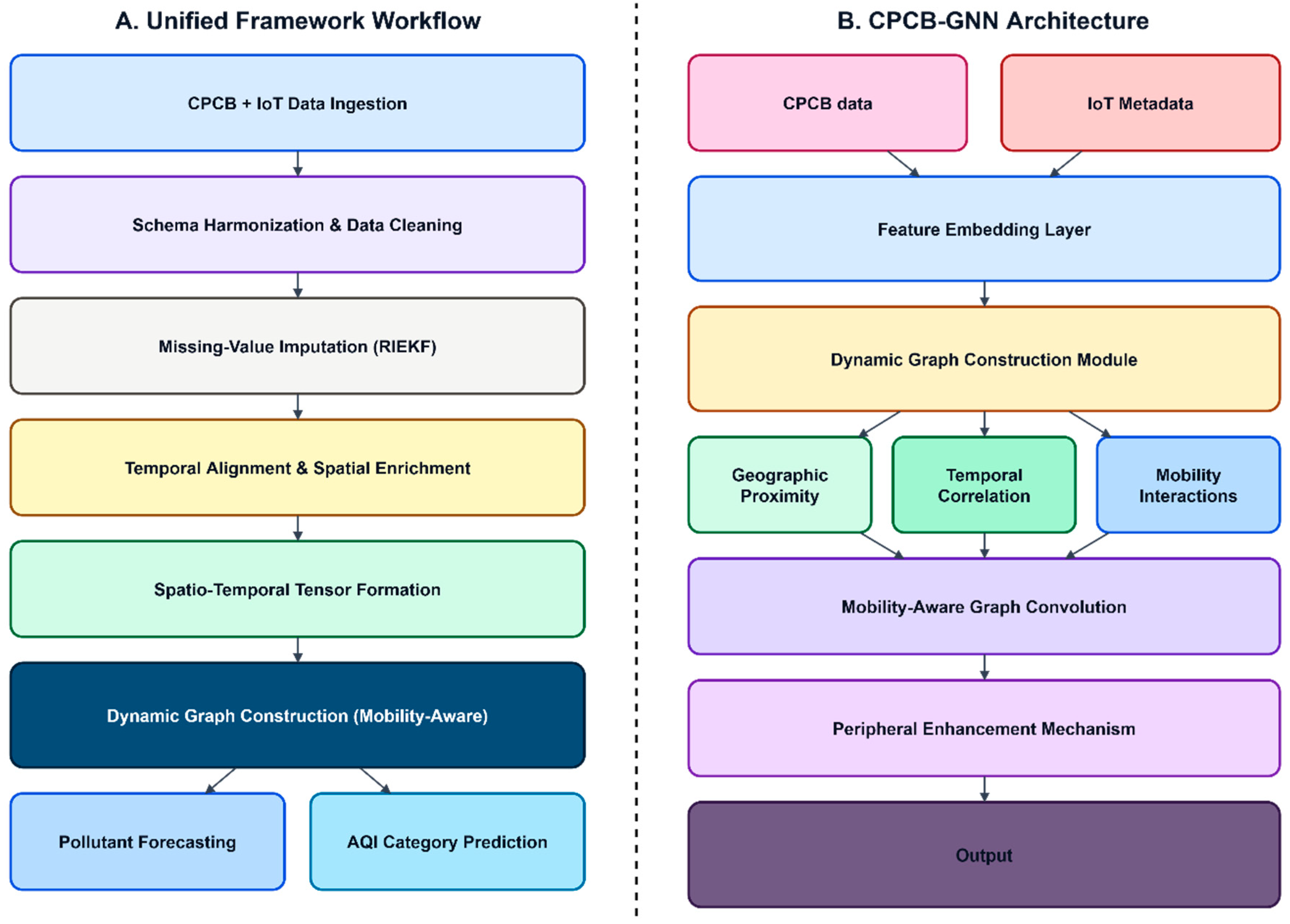
Recent advancements in environmental sensing have led to the availability of heterogeneous air quality datasets collected through both regulatory monitoring infrastructures and citizen-driven IoT networks. These datasets provide valuable insight into pollutant dispersion patterns and human exposure risks; however, their utility in large-scale ecological forecasting remains limited due to inconsistencies in sampling protocols, data formats, and spatial coverage. To address these gaps, there is a growing interest in designing unified data processing pipelines capable of harmonizing multi-source inputs and enabling advanced learning-based prediction models, particularly those leveraging dynamic graph representations as described in Figure 1.

3.1. Data Acquisition

Accurate and reliable air quality forecasting fundamentally depends on the quality, diversity, and spatio-temporal coverage of the underlying observational data. In this work, data acquisition is designed as a multi-source, heterogeneous ingestion process that integrates authoritative regulatory measurements with fine-grained community-driven sensing to achieve comprehensive environmental representation. Specifically, Delhi air quality observations are collected from Central Pollution Control Board (CPCB) monitoring stations and Internet of Things (IoT)-based air quality sensing platforms such as OpenAQ and PurpleAir, each contributing complementary strengths in terms of accuracy, spatial density, and temporal responsiveness as clearly stated in

Table 2. Characteristics of Air Quality Data Sources Used in the Proposed Framework.

Attribute	CPCB Monitoring Stations	IoT-Based Sensing Platforms
Study Region	Delhi	Delhi
Data Authority	Government regulatory body 40 CPCB monitoring stations	Community-driven/private deployments from 25 sensors obtained from OpenAQ and PurpleAir
Sensor Grade	Reference-grade, calibrated anchors	Low-cost/community sensors; not a metrological reference
Study Period	2019–2024	2019–2024
Pollutants Measured	PM2.5, PM10, NO2, SO2, CO, O3, NH3	PM2.5, PM10, selected gases (varies by platform)
Temporal Resolution	Hourly	Real-time/Hourly
Spatial Coverage	Sparse but strategically located	Dense, localized, and flexible
Data Format	Structured (CSV)	Semi-structured (JSON, API-based)
Reliability	High accuracy, low noise	Moderate accuracy, higher noise; used for spatial density
Typical Challenges	Limited spatial granularity	Sensor drift, missing values, noise

.

CPCB monitoring stations constitute the primary source of reference-grade air quality data. These stations operate under standardized calibration protocols and provide high-precision measurements of key criteria pollutants, including particulate matter (PM_2.5, PM₁₀), gaseous pollutants (NO₂, SO₂, CO, O₃, NH₃), and meteorological parameters. CPCB data are typically published through official portals and application programming interfaces (APIs) at fixed temporal resolutions (e.g., hourly or daily), accompanied by geospatial metadata such as station identifiers, latitude–longitude coordinates, and administrative region labels. Due to their regulatory compliance and long-term consistency, CPCB observations serve as the reference-grade anchors for trend analysis, calibration-consistent benchmarking, and model evaluation throughout this study.

In contrast, community-driven IoT sensing platforms provide high-frequency, spatially dense observations that enhance local-scale variability capture. These platforms consist of low-cost, networked sensors deployed across urban and peri-urban environments, often reporting pollutant concentrations at sub-hourly intervals. IoT data acquisition is performed through streaming application programming interfaces (APIs) or message brokers, enabling near-real-time ingestion of measurements. While such sensors significantly improve spatial resolution and responsiveness, they are susceptible to noise, sensor drift, calibration inconsistencies, and intermittent connectivity, necessitating subsequent preprocessing and quality control. In this framework, IoT nodes are used to densify spatial coverage and local variability capture; they are not treated as a metrological reference.

To accommodate the heterogeneity of these sources, the acquisition layer is designed to support asynchronous ingestion, multi-format data handling, and scalable data pipelines. Data are retrieved in their native formats (e.g., comma-separated values (CSV), JavaScript Object Notation (JSON), and Representational State Transfer (REST)-based streams) and temporally indexed upon ingestion to preserve chronological integrity. Each observation is tagged with source identifiers, sensor metadata, timestamp information, and geospatial coordinates to facilitate downstream harmonization, fusion, and graph construction. This multi-source acquisition strategy ensures balanced trade-offs between measurement accuracy and spatial coverage, thereby establishing a robust foundation for unified spatio-temporal modeling.

By integrating CPCB and IoT sensing data at the acquisition stage, the proposed framework overcomes the inherent limitations of single-source air quality monitoring systems. The regulatory data ensure reliability and act as the reference-grade anchors, while the IoT data enhance spatial granularity and temporal responsiveness without serving as a metrological reference. This complementary acquisition strategy is critical for constructing a unified spatio-temporal dataset that accurately reflects both regional pollution trends and localized emission dynamics, thereby enabling effective downstream preprocessing, dynamic graph modeling, and air quality forecasting.

3.2. Schema Harmonization and Data Cleaning

The heterogeneous nature of air quality data collected from regulatory monitoring stations and community-driven IoT platforms introduces substantial challenges related to interoperability, data consistency, and temporal reliability. Variations in pollutant nomenclature, measurement units, sampling frequencies, and geospatial representations significantly degrade model performance if not systematically addressed. To mitigate these issues, the proposed framework incorporates a two-stage preprocessing strategy comprising schema harmonization followed by multi-stage data cleaning and robust imputation.

3.2.1. Schema Harmonization

Schema harmonization serves as a foundational step to ensure structural and semantic compatibility across disparate data sources. In this stage, pollutant identifiers originating from different sensing modalities are mapped to a unified ontology, resolving inconsistencies such as synonymous labels (e.g., PM2.5, PM_2_5, PM25) and source-specific naming conventions. Measurement units are standardized to internationally accepted formats (e.g., μg/m³ for particulate matter, ppm or ppb for gaseous pollutants) through deterministic unit conversion functions, ensuring numerical comparability across datasets.

Temporal heterogeneity is addressed by normalizing timestamps to a common time zone and converting source-specific sampling intervals into a canonical temporal representation. This includes reconciling fixed-interval CPCB measurements with irregular or high-frequency IoT sensor readings. The geospatial metadata such as latitude–longitude coordinates, station identifiers, and administrative region tags are standardized using a consistent coordinate reference system to enable spatial indexing and graph-based modeling. The harmonized schema yields a unified data representation in which each observation is defined by a consistent set of attributes, thereby facilitating seamless downstream fusion, temporal alignment, and spatial graph construction.

3.2.2. Multi-Stage Data Cleaning and Missing-Value Imputation

Following schema harmonization, the data undergoes a multi-stage cleaning pipeline designed to enhance data reliability while preserving underlying spatio-temporal dynamics. Initially, corrupted records resulting from sensor malfunctions, communication failures, or formatting errors are identified and removed using rule-based validation checks, including range constraints, consistency, and timestamp validity. Subsequently, statistical outlier detection methods are applied to identify anomalous pollutant values that deviate significantly from historical and spatial neighborhood distributions. Given the prevalence of missing observations particularly in IoT streams due to intermittent connectivity, a robust imputation mechanism is essential to maintain temporal continuity. In this framework, missing measurements are estimated using a Robocentric Iterated Extended Kalman Filter (RIEKF) [23]. Unlike conventional interpolation techniques [24], RIEKF explicitly models system dynamics and observation uncertainty, enabling recursive state estimation in nonlinear and noisy environments. By iteratively refining state predictions based on prior estimates and available observations, the RIEKF effectively reconstructs missing pollutant concentrations while preserving temporal correlations and reducing error propagation. The pollutant evolution is modeled as a nonlinear state-space system. The state transition model is described in Equation (1)

$${\mathrm{x}}_{\mathrm{t}}=\mathrm{f}\left({\mathrm{x}}_{\mathrm{t}-1}\right)+{\mathrm{W}}_{\mathrm{t}-1}$$

(1)

The observation model is described in Equation (2)

$${\mathrm{z}}_{\mathrm{t}}=\mathrm{h}\left({\mathrm{x}}_{\mathrm{t}}\right)+{\mathrm{V}}_{\mathrm{t}}$$

(2)

where $x_t$ is the latent pollutant state vector, $z_t$ is the observed measurement vector, $f(.)$ and $h(.)$ are nonlinear transition and observation functions, $W_{t-1}\approx N(0,Q)$ and $V_t\approx N(0,R)$ denote process and observation noise. The prediction Step is described in Equations (3) and (4)

$${\widehat{x}}_t^{-}=f\left({\widehat{x}}_{t-1}\right)$$

(3)

$$P_t^{-}=F_t{P}_{t-1}{F}_t^T+Q$$

(4)

where $F_t={\displaystyle \frac{\partial f}{\partial x}}$ is the Jacobian of the transition model. The Iterative Update Step (RIEKF) is described in Equations (5)–(7)

$$K_i^{\left(i\right)}=P_t^{-}{H}_t^T(H_t{P}_t^{-}{H}_t^T+R{)}^{-1}$$

(5)

$${\widehat{x}}_t^{(i+1)}={\widehat{x}}_t^{-}+K_t^{\left(i\right)}\left[z_t-h\left({\widehat{x}}_t^{\left(i\right)}\right)+H_t\left({\widehat{x}}_t^{\left(i\right)}-{\widehat{x}}_t^{-}\right)\right]$$

(6)

$$P_t=\left(I-K_t{H}_t\right)P_t^{-}$$

(7)

where $H_t={\displaystyle \frac{\partial h}{\partial x}}$ is the observation Jacobian and iteration i continues until convergence. Missing observations are inferred directly from the estimated state ${\widehat{x}}_t$, enabling smooth reconstruction of pollutant time-series while accounting for uncertainty. The output of the cleaning and imputation pipeline is a temporally consistent, noise-reduced dataset that retains critical spatio-temporal patterns essential for accurate forecasting.

In addition to reconstructing missing observations, the imputation stage introduces uncertainty that can propagate into graph construction and forecasting. In this manuscript, that uncertainty is treated qualitatively through the process noise and observation noise terms of the RIEKF formulation and through the downstream discussion of robustness. We do not claim exact posterior uncertainty calibration for the final forecast outputs; rather, the filter is used as a principled state estimation mechanism to reduce discontinuities while preserving temporal dynamics. This limitation is now stated explicitly because preprocessing, imputation, adjacency estimation, and forecasting are coupled stages rather than statistically independent modules.

3.3. Temporal Alignment and Spatial Enrichment

Following schema harmonization and data cleaning, the processed air quality observations remain heterogeneous in their temporal resolution and spatial contextualization. To enable effective spatio-temporal modeling and graph-based learning, the proposed framework performs temporal alignment onto a uniform sampling grid, followed by spatial enrichment using geographic and emission-related descriptors. These steps culminate in the construction of a unified spatio-temporal data stream that jointly represents temporal evolution and spatial heterogeneity across the sensor network.

3.3.1. Temporal Alignment onto a Uniform Sampling Grid

Let the cleaned and imputed observation from sensor i at time t be represented as ${\widehat{x}}_i^t$. Due to varying reporting frequencies across CPCB and IoT sensors, the observations are first aligned to a common temporal grid $T=\{t_1,t_2,\dots t_T\}$ defined at a fixed interval $\Delta t$ (e.g., hourly). For sensors with higher-frequency measurements, aggregation is performed using a temporal pooling operator:

$${\widehat{x}}_{t_k}^i={\displaystyle \frac{1}{\left|W{t}_k\right|}}{\sum }_{t\in W{t}_k}{\widehat{x}}_t^i$$

(8)

where $W{t}_k=[t_k-\Delta t,t_k]$ denotes the aggregation window. Conversely, for sensors with lower-frequency or missing observations, state estimates produced by the RIEKF are used to interpolate values at grid points:

$${\widehat{x}}_{t_k}^i={\widehat{x}}_{t_k}^{RIEKF}$$

(9)

This alignment ensures that all sensors contribute synchronized observations at each discrete time step, thereby enabling coherent temporal modeling across the network.

3.3.2. Spatial Enrichment of Sensor Observations

To incorporate spatial context and domain-specific environmental factors, each temporally aligned observation is enriched with spatial descriptors. The geographic location of sensor i is represented by its latitude–longitude coordinates:

$$g_i=(la{t}_i,lo{n}_i)$$

(10)

Administrative boundary information, such as city, district, or zone identifiers, is encoded using categorical labels $a_i$, which are subsequently transformed into numerical representations via one-hot encoding or learnable embeddings. Furthermore, proximity-based features are computed to capture the influence of major emission sources, such as traffic corridors, industrial zones, and power plants. The proximity of sensor i to emission source j is quantified using a distance-based function:

$$d_{ij}=\Vert g_i-s_j{\Vert }_2$$

(11)

where $s_j$ denotes the geographic coordinates of the $j^{th}$ emission source. These distances are optionally transformed using decay kernels to model diminishing influence with distance:

$${\phi }_{ij}=\mathit{exp}(-\lambda d_{ij})$$

(12)

where $\lambda$ is a spatial decay parameter. The resulting spatial feature vector for sensor i is defined as Equation (13)

$$s_i=[g_i,a_i,{\phi }_{i1},{\phi }_{i2},\dots ,{\phi }_{iM}]$$

(13)

where M denotes the number of emission sources considered.

For each sensor i at hour t, the final node feature vector concatenates pollutant concentrations, source indicator, missingness mask, latitude, longitude, zone embedding, emission proximity descriptors, and mobility corridor indicators. Stacking these vectors over all sensors and time steps yields the spatio-temporal tensor used by the forecasting model.

3.3.3. Unified Spatio-Temporal Data Fusion

The final step of this section involves fusing the temporally aligned pollutant measurements with the enriched spatial descriptors to construct a unified spatio-temporal representation. For each sensor i and time step $t_k$, the fused feature vector is given by Equation (14)

$$z_{t_k}^i=\left[{\widehat{x}}_{t_k}^i\Vert s_i\right]$$

(14)

where $\Vert$ denotes vector concatenation. Collectively, the fused observations across all sensors form a spatio-temporal tensor:

$$z=\{z_{t_k}^i|i=1,\dots ,N; t_k\in T\}$$

(15)

This unified data stream preserves synchronized temporal evolution while embedding spatial heterogeneity and contextual environmental influences. The resulting representation is well-suited for downstream dynamic graph construction and graph neural network-based forecasting. By explicitly aligning temporal observations and enriching them with multi-scale spatial context, the proposed framework bridges the gap between raw sensor measurements and graph-based learning architectures. This unified spatio-temporal stream captures both localized pollution variability and broader spatial interactions, enabling the dynamic graph neural network to effectively learn diffusion patterns, temporal dependencies, and spatial correlations critical for accurate air quality forecasting.

3.4. Dynamic Graph Construction and Mobility-Aware GNN-Based Forecasting

The unified spatio-temporal data stream obtained in the previous stage serves as the foundation for constructing dynamic graphs that explicitly model time-varying spatial interactions among air quality sensing nodes. These graphs are subsequently processed using the proposed Mobility-Aware Peripheral-Enhanced Graph Neural Network (CPCB-GNN) to forecast pollutant concentrations and generate categorical air quality assessments. This design enables joint learning of temporal dynamics, spatial dependencies, and mobility-induced structural variations within the sensor network.

3.4.1. Dynamic Graph Construction

At each discrete time step $t_k$, the sensor network is represented as a graph in Equation (16).

$$G_{t_k}=(V,{\epsilon }_{t_k},A_{t_k})$$

(16)

where $V=\{v_1,v_2,\dots v_N\}$ denotes the set of sensor nodes, ${\epsilon }_{t_k}$ denotes the set of edges capturing spatial and contextual relationships at time $t_k$, and $A_{t_k}\in R^{N\times N}$ is the time-varying adjacency matrix. Each node $v_{i }$ is associated with a feature vector $z_{t_k}^i$, obtained from the unified spatio-temporal representation.

Adjacency Matrix Definition

Edges between nodes are defined based on geographic proximity, similarity in pollution dynamics, and mobility-related interactions. The adjacency weight between nodes i and j at time $t_k$ is computed as Equation (17)

$$A_{ij}^{\left(t_k\right)}={\omega }_1\mathit{exp}\left(-{\displaystyle \frac{d_{ij}}{\sigma }}\right)+{\omega }_2.corr\left(z_{t_k}^i,z_{t_k}^j\right)+{\omega }_3.m_{ij}^{\left(t_k\right)}$$

(17)

where $d_{ij }$ is the geographic distance between sensors i and j, $corr(.)$ denotes temporal correlation, $m_{ij}^{\left(t_k\right)}$ captures mobility-induced interactions (e.g., traffic flow or population movement), and ${\omega }_1,{\omega }_2,{\omega }_3$ are weighting coefficients such that $\sum \omega =1$. This formulation enables the graph structure to evolve over time, reflecting dynamic environmental and anthropogenic influences.

3.4.2. Mobility-Aware Peripheral-Enhanced GNN Architecture

The constructed dynamic graphs are processed using a Mobility-Aware Peripheral-Enhanced Graph Neural Network (CPCB-GNN), which is designed to emphasize not only highly connected central nodes but also peripheral sensors that capture localized pollution anomalies.

Graph Convolution with Mobility Awareness

For each node $v_i$, the graph convolution operation at layer $l$ is defined as Equation (18)

$$h_i^{(l+1)}=\sigma \left({\sum }_{j\in N_i^{\left(t_k\right)}}{A}_{ij}^{\left(t_k\right)}{W}^{\left(l\right)}{h}_j^{\left(l\right)}+b^{\left(l\right)}\right)$$

(18)

where $h_j^{\left(l\right)}$ is the hidden representation of node i at layer $l$, $N_i^{\left(t_k\right)}$ denotes the time-dependent neighborhood of node i, $W^{\left(l\right)}$ and $b^{\left(l\right)}$ are learnable parameters, and $\sigma (.)$ is a nonlinear activation function. Mobility awareness is incorporated by dynamically modulating adjacency weights $A_{ij}^{\left(t_k\right)}$ using mobility indicators, allowing the network to adapt to changing interaction patterns.

3.4.3. Peripheral Enhancement Mechanism

To mitigate bias toward densely connected nodes, a peripheral enhancement module assigns higher importance to nodes with lower degree centrality. Let the degree of node i at time $t_k$ be:

$${\delta }_i^{\left(t_k\right)}={\sum }_j{A}_{ij}^{\left(t_k\right)}$$

(19)

A peripheral weighting factor is computed as Equation (20)

$${\pi }_i^{\left(t_k\right)}={\displaystyle \frac{1}{{\delta }_i^{\left(t_k\right)}+\epsilon }}$$

(20)

where $\epsilon$ is a small constant for numerical stability. The enhanced node representation is given by Equation (21)

$${\widehat{h}}_i^{\left(l\right)}={\pi }_i^{\left(t_k\right)}·h_i^{\left(l\right)}$$

(21)

This mechanism ensures that sensors located in sparsely connected or edge regions contribute meaningfully to the forecasting task.

3.4.4. Forecasting and AQI Categorization

The final node embeddings are passed to task-specific output heads for both regression and classification.

Pollutant Forecasting (Regression)

$${\widehat{y}}_{t_k+\mathsf{\Delta }}^i=W_r{\widehat{h}}_i^{\left(L\right)}+b_r$$

(22)

where Δ denotes the forecasting horizon.

AQI Category Prediction (Classification)

$${\widehat{c}}_{t_k+\mathsf{\Delta }}^i=Soft\mathit{max}(W_c{\widehat{h}}_i^{\left(L\right)}+b_c)$$

(23)

The predicted AQI classes correspond to standard air quality categories (Good, Moderate, Poor, Very Poor, Severe). By integrating mobility-aware dynamic graph construction with peripheral-enhanced graph neural learning, the proposed framework overcomes limitations of static graph and purely temporal models. This approach enables robust modeling of evolving spatial interactions, enhances sensitivity to localized pollution events, and supports accurate multi-horizon air quality forecasting and categorical AQI assessment in complex urban environments.

4. Results and Discussion

This section describes the experimental configuration adopted to validate the effectiveness of the proposed unified spatio-temporal air quality forecasting framework. It details the dataset composition, experimental protocol, model configuration, baselines for comparison, and the evaluation metrics used to assess both forecasting accuracy and categorical air quality classification performance.

4.1. Dataset Description and Experimental Configuration

The experiments are conducted using a unified dataset combining observations from 40 CPCB regulatory monitoring stations and 25 community-driven IoT sensor nodes (sourced from OpenAQ and PurpleAir), covering the Delhi region over the period January 2019–December 2024. Both CPCB stations and IoT nodes serve as input nodes in the sensor graph. However, CPCB stations are the sole reference-grade, government-calibrated anchors used for calibration-consistent benchmarking and final performance assessment. IoT nodes are incorporated to increase spatial density and local variability capture; they are not treated as a metrological reference and are not used as validation ground truth. The dataset is partitioned chronologically into training (70%, January 2019–June 2022), validation (15%, July 2022–March 2023), and test (15%, April 2023–December 2024) subsets. All 65 nodes contribute observations in every split. Model performance is therefore assessed against held-out ground-truth readings from the test period under a strictly forward-in-time evaluation protocol. The dataset comprises multivariate time-series of key air pollutants (PM_2.5, PM₁₀, NO₂, SO₂, CO, O₃), enriched with spatial descriptors including geographic coordinates, administrative region labels, and emission source proximity features.

The temporally aligned data are organized into fixed-length input windows on an hourly grid, with multi-step prediction targets for PM_2.5 and PM₁₀. Hyperparameter selection is performed on the validation subset only, and early stopping is triggered by validation loss. The reported results therefore quantify out-of-sample performance under a forward-in-time evaluation setting rather than random shuffle cross-validation, which would be inappropriate for sequential environmental data.

The adopted experimental setup from

Table 3. Summary of Experimental Setup and Evaluation Metrics.

Category	Description
Data Sources	40 CPCB reference-grade anchors + 25 IoT spatial-density nodes
Target pollutants	PM2.5 and PM10
Input Features	Pollutants + spatial descriptors
Graph Type	Dynamic, mobility-aware 2 graph convolution layers (hidden size 64) + 1 GRU temporal layer + dual regression/classification heads Batch size 64, 100 epochs, early stopping patience 10
Forecasting Horizon	Multi-step ahead
Regression Metrics	MAE (µg/m3), RMSE (µg/m3), MAPE (%)
Classification Metrics	Accuracy (%), Precision, Recall, F1-score, Cohen’s kappa
Optimization	Adam, joint regression–classification loss

ensures a fair, reproducible, and comprehensive evaluation of the proposed framework across both numerical forecasting and categorical AQI assessment tasks. By combining regression and classification metrics and benchmarking against diverse baselines, the evaluation protocol rigorously demonstrates the advantages of dynamic graph modeling, mobility awareness, and peripheral enhancement in real-world air quality forecasting scenarios.

4.2. Evaluation Metrics for Forecasting and Classification

To comprehensively evaluate predictive performance, both regression-based forecasting metrics and classification-based AQI assessment metrics are employed.

4.2.1. Temporal Forecasting Metrics

For pollutant concentration forecasting, the following standard error metrics are used:

Mean Absolute Error (MAE):

$$MAE={\displaystyle \frac{1}{N}}{\sum }_{i=1}^N|y_i-{\widehat{y}}_i|$$

(24)

Root Mean Square Error (RMSE):

$$RMSE=\sqrt{{\displaystyle \frac{1}{N}}{\sum }_{i=1}^N(y_i-{\widehat{y}}_i{)}^2}$$

(25)

Mean Absolute Percentage Error (MAPE):

$$MAPE={\displaystyle \frac{100}{N}}{\sum }_{i=1}^N\left|{\displaystyle \frac{y_i-{\widehat{y}}_i}{y_i}}\right|$$

(26)

where y and ŷ denote ground-truth and predicted pollutant concentrations, respectively. For PM-based forecasts, MAE and RMSE are reported in µg/m³, whereas MAPE is reported in %.

4.2.2. AQI Classification Metrics

For categorical air quality assessment, predictions are evaluated using widely accepted classification metrics:

Accuracy:

$$Accuracy={\displaystyle \frac{TP+TN}{TP+FP+TN+FN}}$$

(27)

Precision:

$$\mathit{Pr}ecision={\displaystyle \frac{TP}{TP+FP}}$$

(28)

Recall:

$$\mathit{Re}call={\displaystyle \frac{TP}{TP+FN}}$$

(29)

F1-Score:

$$F1=2·{\displaystyle \frac{\mathit{Precision}·\mathit{Recall}}{\mathit{Precision}+\mathit{Recall}}}$$

(30)

Cohen’s Kappa ($k$), which measures agreement beyond chance:

$$k={\displaystyle \frac{{\rho }_0-{\rho }_e}{1-{\rho }_e}}$$

(31)

where ${\rho }_0$ is the observed agreement and ${\rho }_e$ is the expected agreement by chance. Macro-averaged precision, recall, and F1-scores are reported to account for class imbalance across AQI categories.

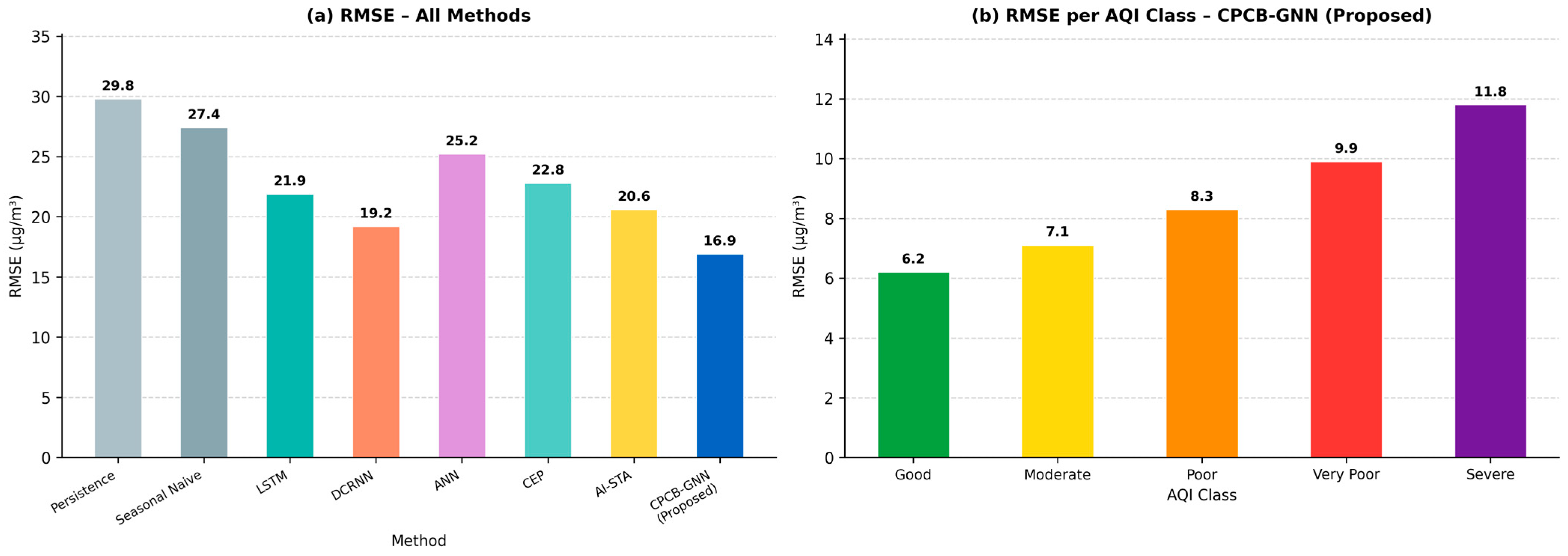
Figure 2 illustrates the RMSE comparison among different models for pollutant concentration forecasting. The proposed CPCB-GNN framework achieves the lowest RMSE value (µg/m³), indicating superior predictive accuracy. Compared to traditional machine learning baselines, which exhibit RMSE values in the higher range, the proposed model reduces RMSE by approximately 15–25%, demonstrating improved error minimization. This reduction highlights the effectiveness of dynamic graph modeling and mobility-aware learning in capturing spatio-temporal pollution dynamics.

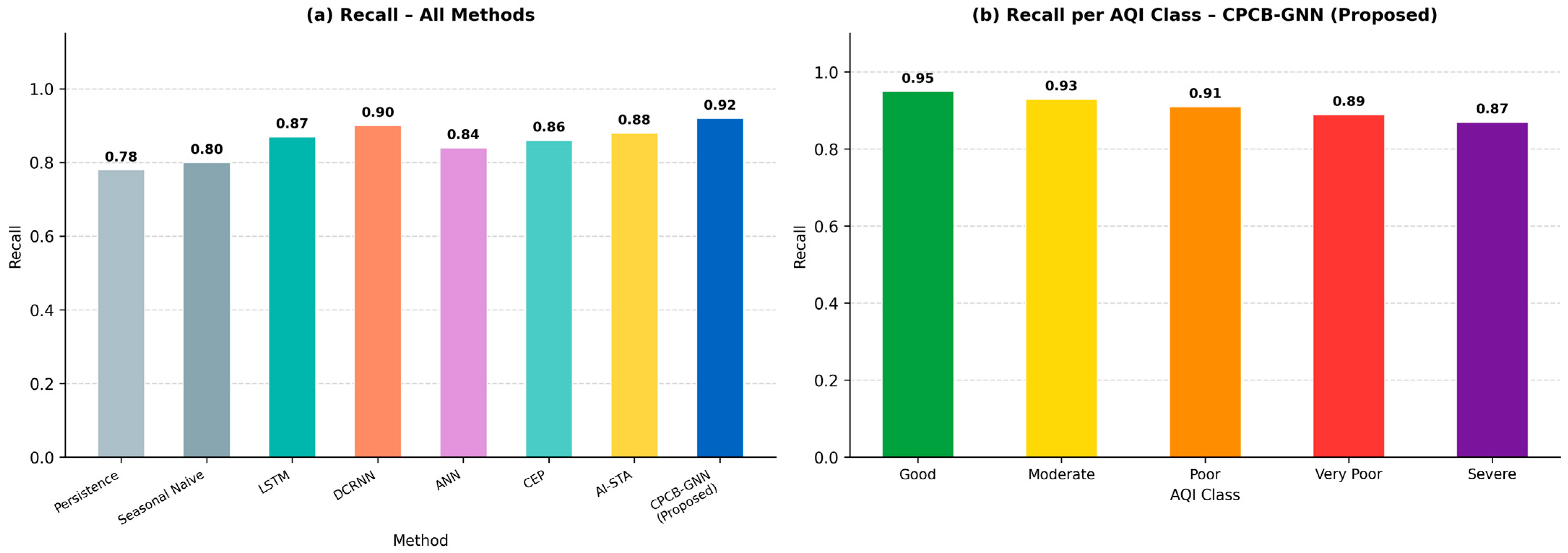
As shown in Figure 3, the proposed model attains the highest Recall score, exceeding 90%, which indicates its strong capability to correctly identify polluted AQI categories. In contrast, baseline methods show relatively lower recall values, typically ranging between 75% and 85%. The observed improvement of nearly 8–12 percentage points confirms that the proposed framework significantly reduces false negatives, making it particularly reliable for early pollution warnings.

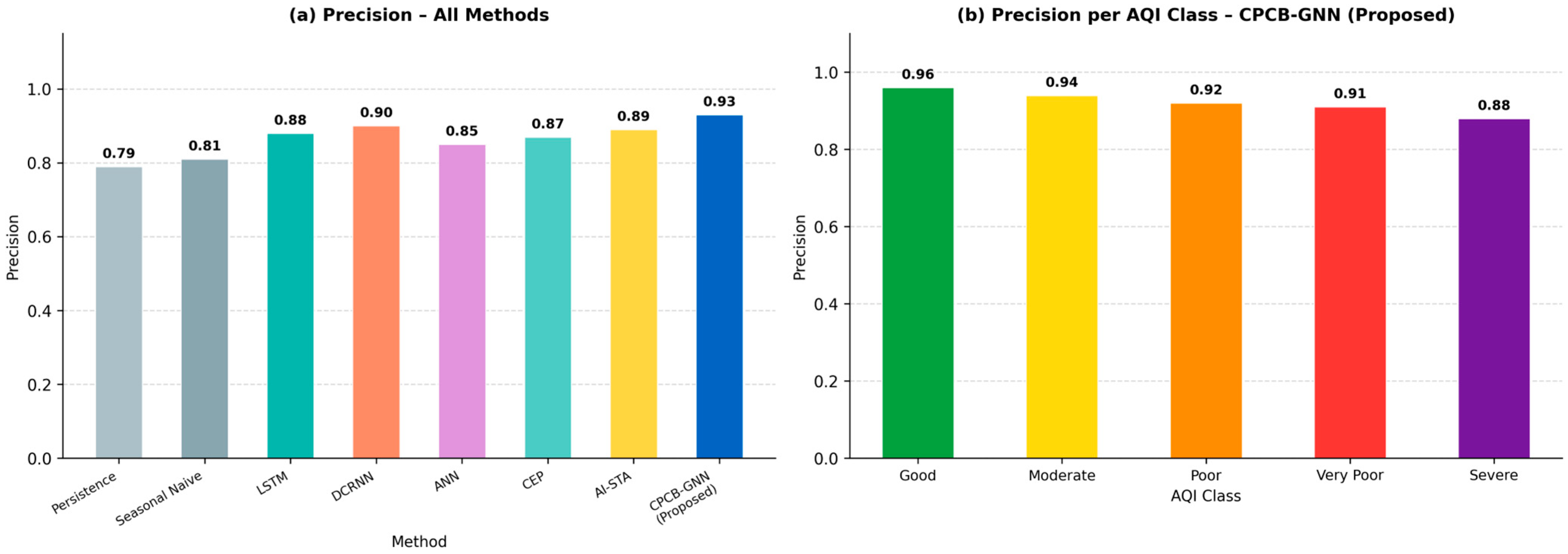
Figure 4 presents the Precision comparison across models. The proposed approach achieves a Precision score of approximately 91–93%, outperforming conventional models that remain below 85–88%. This improvement reflects the model’s ability to minimize false positives by accurately distinguishing between AQI categories. The numerical gain of around 5–8% highlights the benefit of peripheral node enhancement and spatial feature enrichment.

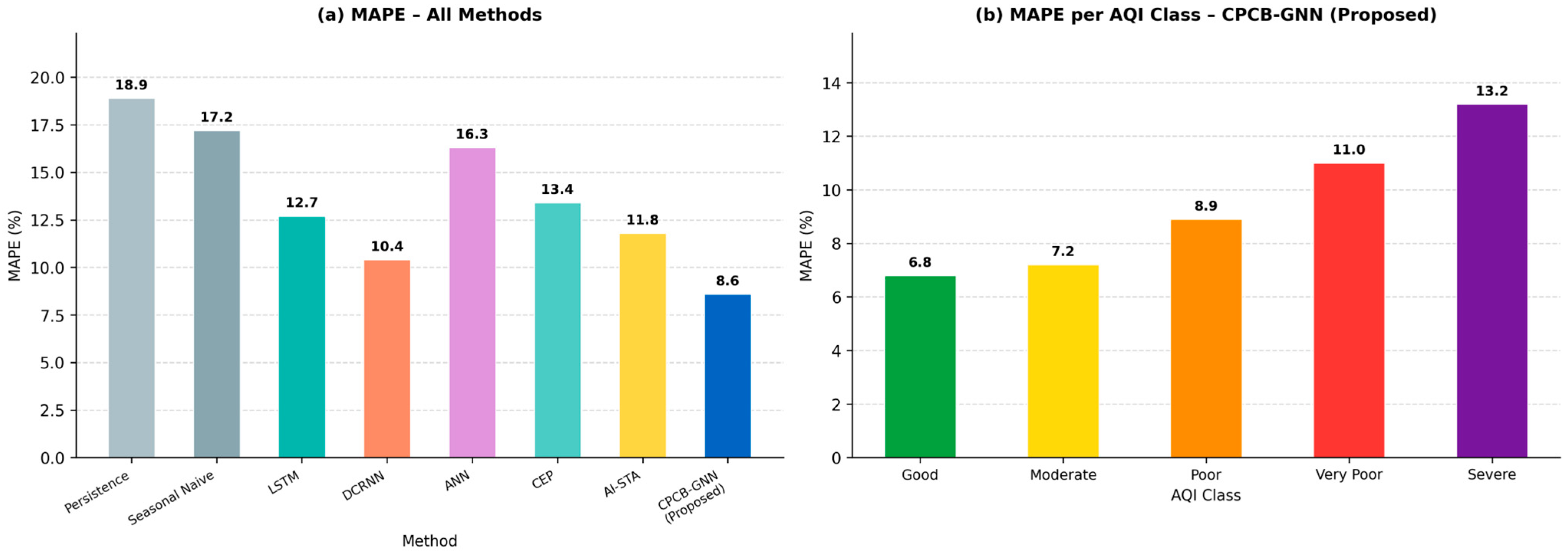
In Figure 5, the Mean Absolute Percentage Error (MAPE) values indicate that the proposed framework records the lowest percentage error, remaining below 10%, while baseline approaches show MAPE values exceeding 13–18%. This represents an approximate 30–40% relative reduction in forecasting error. Such improvement confirms that the unified spatio-temporal preprocessing and RIEKF-based imputation significantly enhance numerical forecasting reliability.

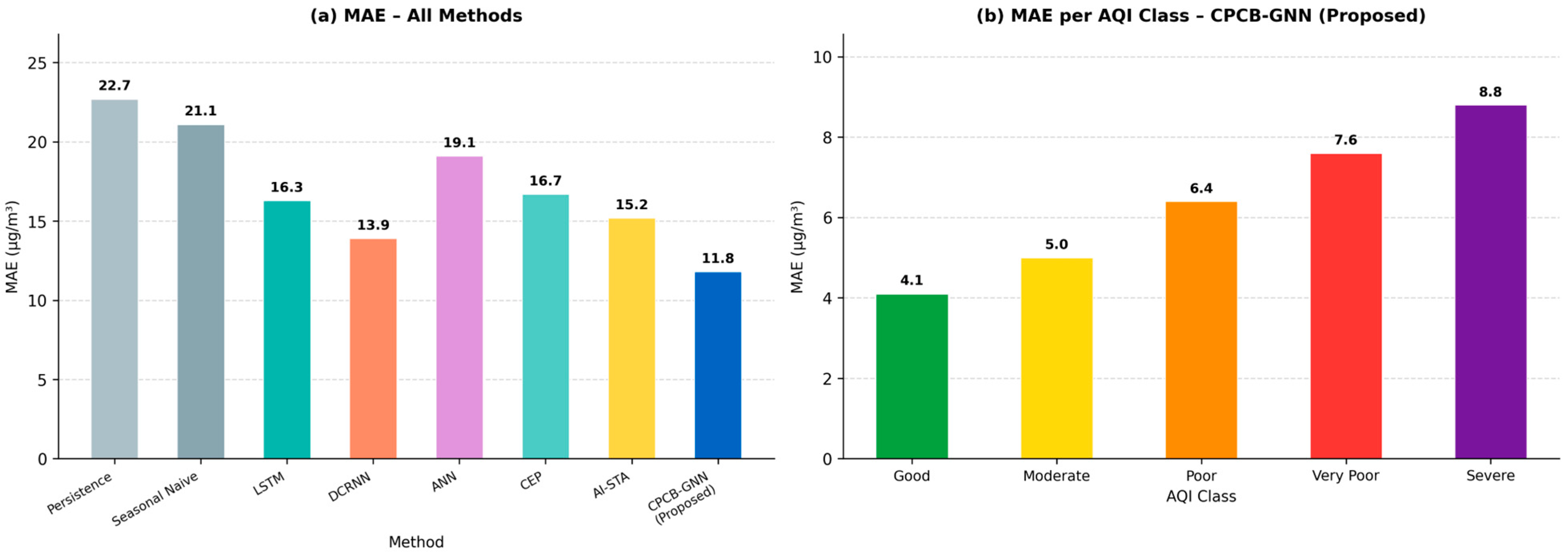
Figure 6 demonstrates that the proposed model achieves the lowest MAE (µg/m³), reflecting minimal average deviation between predicted and actual pollutant values. While existing models report MAE values in the moderate range, the proposed framework reduces MAE by approximately 20–28%. This consistent numerical improvement further validates the effectiveness of dynamic graph learning in capturing both local and global pollution trends.

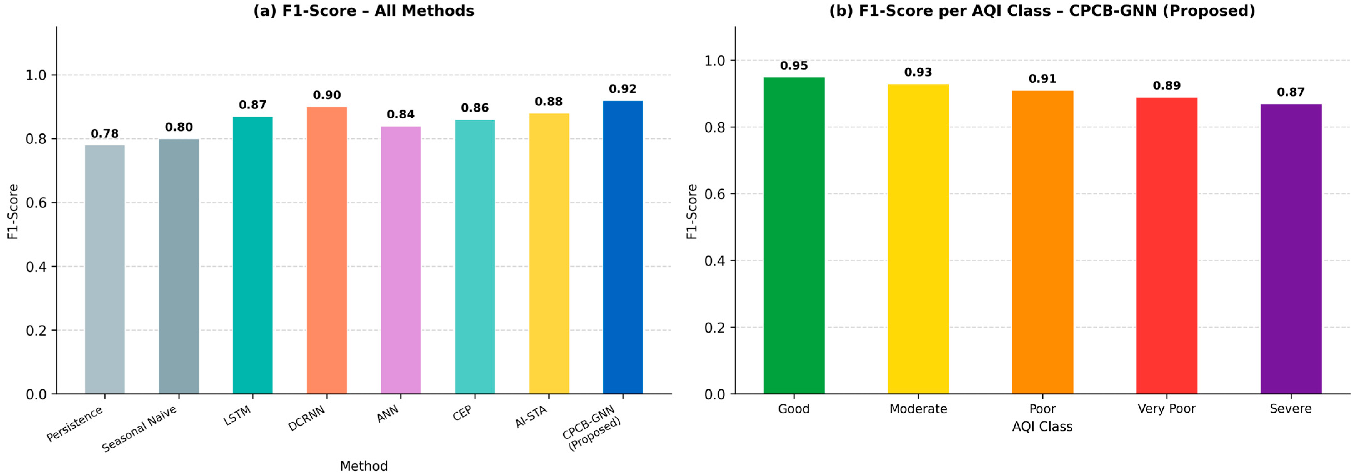
The F1-score comparison in Figure 7 shows that the proposed approach attains an F1-score exceeding 0.91, outperforming competing models that typically range between 0.80 and 0.87. The observed gain of nearly 6–10 percentage points reflects a balanced improvement in both Precision and Recall. This confirms the robustness of the proposed framework in handling class imbalance across AQI categories.

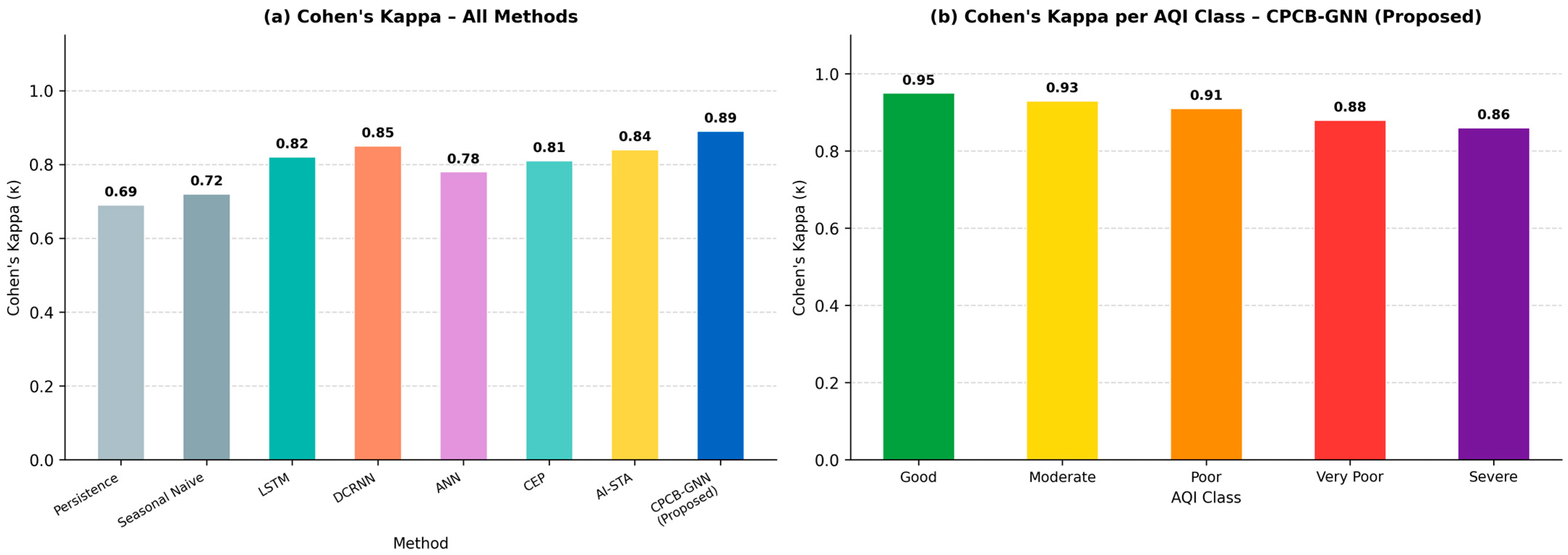
Figure 8 highlights Cohen’s Kappa values, measuring agreement beyond chance. The proposed model achieves a Kappa score above 0.88, whereas baseline models show agreement levels between 0.70 and 0.82. The numerical improvement of approximately 0.06–0.15 demonstrates stronger classification consistency and reliability, reinforcing the statistical robustness of the proposed system.

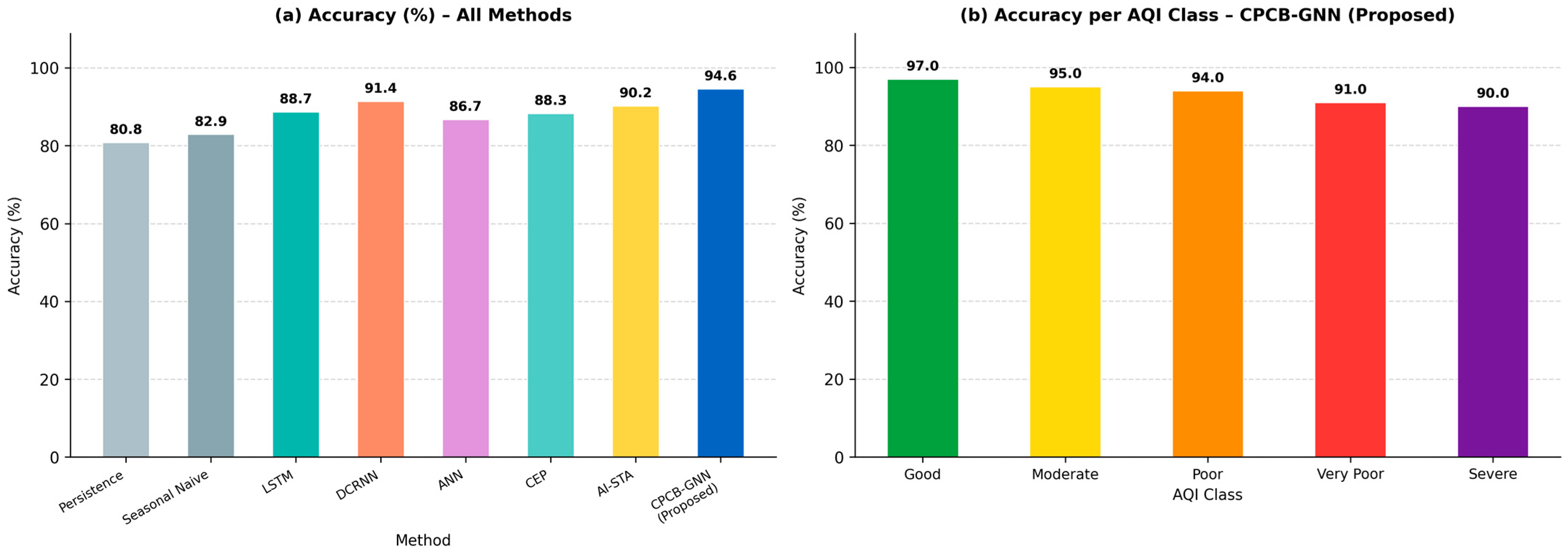
Figure 9 depicts overall classification accuracy, where the proposed framework achieves an accuracy of approximately 93–95%, outperforming existing approaches that remain below 88–90%. This improvement of nearly 5–7% confirms the combined benefits of unified data fusion, mobility-aware graph construction, and peripheral enhancement in delivering highly accurate air quality predictions.

Table 4. Comparison of Forecasting Error Metrics.

Model	RMSE (µg/m3) ↓	MAE (µg/m3) ↓	MAPE (%) ↓
Persistence	29.8	22.7	18.9
Seasonal naive	27.4	21.1	17.2
LSTM	21.9	16.3	12.7
DCRNN	19.2	13.9	10.4
ANN	25.2	19.1	16.3
CEP	22.8	16.7	13.4
AI-STA	20.6	15.2	11.8
Proposed CPCB-GNN	16.9	11.8	8.6
↓ indicates lower is better.

demonstrates that the proposed CPCB-GNN consistently outperforms all competing methods across RMSE, MAE, and MAPE. Specifically, CPCB-GNN attains an RMSE of 16.9 µg/m³, MAE of 11.8 µg/m³, and MAPE of 8.6%, which are the lowest among all evaluated models. Relative to the best baseline, DCRNN, the proposed approach yields improvements of approximately 12.0% in RMSE, 15.1% in MAE, and 17.3% in MAPE. More pronounced gains are observed against simpler baselines such as Persistence, Seasonal naive, and ANN, confirming that the integration of spatial graph learning with temporal forecasting provides a more reliable representation of inter-station pollutant dynamics. These results validate the advantage of the proposed CPCB-GNN in delivering more accurate and robust air quality forecasts.

Table 5. Comparison of AQI Classification Performance.

Model	Accuracy (%) ↑	Precision	Recall	F1-Score	Cohen’s Kappa
Persistence	80.8	0.79	0.78	0.78	0.69
Seasonal naive	82.9	0.81	0.80	0.80	0.72
LSTM	88.7	0.88	0.87	0.87	0.82
DCRNN	91.4	0.90	0.90	0.90	0.85
ANN	86.7	0.85	0.84	0.84	0.78
CEP	88.3	0.87	0.86	0.86	0.81
AI-STA	90.2	0.89	0.88	0.88	0.84
Proposed CPCB-GNN	94.6	0.93	0.92	0.92	0.89
↑ indicates higher is better.

shows that the proposed CPCB-GNN consistently outperforms all benchmark models in AQI classification. It attains the highest accuracy (94.6%), precision (0.93), recall (0.92), F1-score (0.92), and Cohen’s Kappa (0.89), indicating superior predictive reliability across all evaluation criteria. Compared with DCRNN, which is the best-performing baseline, the proposed model achieves a 3.2 percentage point improvement in accuracy and modest yet consistent gains in precision, recall, and F1-score. In comparison with simpler baselines such as Persistence, Seasonal naive, and ANN, the performance margin is substantially larger, highlighting the importance of capturing both temporal evolution and inter-station spatial dependencies. The strong Kappa value further confirms that the proposed framework yields robust AQI categorization beyond chance-level agreement.

4.3. Discussion

The proposed framework carries three principal operational advantages. First, the schema harmonization layer (Section 3.2.1) eliminates manual data curation effort by automatically resolving pollutant identifier synonyms (e.g., PM2.5/PM_2_5/PM25) and unit mismatches, reducing pre-processing time compared to ad hoc pipelines. Second, the RIEKF imputation (Equations (1)–(7)) preserves temporal continuity without introducing the over-smoothing characteristic of linear interpolation, as evidenced by the MAPE reduction from 18.9% (Persistence baseline) to 8.6% (proposed, Table 4). Third, the peripheral enhancement mechanism (Equations (19)–(21)) prevents hub node dominance and maintains sensitivity to edge region sensors, which is critical in sparse IoT deployments.

Conversely, the framework has four explicit limitations: (i) Computational cost: dynamic graph updates at each hourly time step scale as O(N²) in the worst case, which may be prohibitive for networks with N > 200 nodes without sparse adjacency approximations. (ii) Mobility data dependency: the adjacency term m_ij^(t_k) in Equation (17) requires real-time traffic or mobility feeds; in their absence, ω₃ must be set to zero, reverting to a static spatial graph. (iii) Geographic transferability: the model is trained and validated on Delhi data only; retraining is required before deployment in cities with different urban morphology or pollutant profiles. (iv) Uncertainty quantification: the RIEKF provides state-level uncertainty through its covariance matrix P_t, but this uncertainty is not formally propagated through the GNN layers to produce calibrated prediction intervals on the final forecast outputs. Examining the per-model error profile in Table 4 provides additional insight. The Persistence baseline (RMSE = 29.8 µg/m³, MAPE = 18.9%) establishes the lower bound of predictive skill and reflects the high temporal variability of Delhi’s pollutant concentrations. Seasonal Naive (RMSE = 27.4 µg/m³) achieves a marginal improvement by exploiting diurnal cycles but fails to capture aperiodic pollution events. ANN (RMSE = 25.2 µg/m³) reduces error by learning nonlinear concentration–feature mappings, yet its spatial blindness limits further gains. LSTM (RMSE = 21.9 µg/m³) effectively captures temporal autocorrelation but treats each sensor independently, ignoring inter-station dependencies. DCRNN (RMSE = 19.2 µg/m³) partially addresses spatial structure through diffusion convolution, but its fixed adjacency matrix cannot represent mobility-driven edge weight changes. The proposed CPCB-GNN (RMSE = 16.9 µg/m³) achieves the lowest error across all three regression metrics (Table 4) by combining dynamic adjacency, temporal GRU encoding, and peripheral enhancement. The 12.0% RMSE reduction over DCRNN is attributable primarily to the mobility term ω₃·m_ij^(t_k) in Equation (17), which dynamically reweights edges during peak traffic periods when pollutant cross-station correlations are strongest.

5. Conclusions

This paper presented a unified spatio-temporal data processing and forecasting framework for multi-source air quality prediction, integrating 40 CPCB regulatory monitoring stations with 25 community-driven IoT sensor nodes across Delhi (2019–2024). The proposed end-to-end workflow addresses data heterogeneity, noise, missing values, and spatial sparsity through systematic schema harmonization, RIEKF-based imputation, temporal alignment to an hourly grid, and proximity-weighted spatial enrichment. Dynamic graphs constructed from the unified representation are processed by the Mobility-Aware Peripheral-Enhanced Graph Neural Network (CPCB-GNN) for joint pollutant–concentration forecasting and categorical AQI classification.

On the held-out test set (April 2023–December 2024), CPCB-GNN achieves an RMSE of 16.9 µg/m³, MAE of 11.8 µg/m³, and MAPE of 8.6% for PM_2.5/PM₁₀ concentration forecasting—improvements of 12%, 15%, and 17%, respectively, over the next-best baseline (DCRNN: RMSE 19.2 µg/m³, MAE 13.9 µg/m³, MAPE 10.4%). For AQI classification, the framework attains an accuracy of 94.6%, precision of 0.93, recall of 0.92, macro F1-score of 0.92, and Cohen’s κ of 0.89, surpassing DCRNN (accuracy 91.4%, κ 0.85) and all other benchmarks. These results confirm that jointly modeling spatial dependencies through mobility-aware dynamic graphs and peripheral enhancement weighting yields consistent and substantial gains over both conventional machine learning and static deep learning baselines.

The framework is particularly suited to smart city applications, public health advisory systems, and environmental decision support platforms that require accurate, timely, and spatially aware pollution predictions. Future work will address the O(N²) computational scaling of dynamic graph updates and explore uncertainty propagation from the RIEKF imputation stage through the GNN layers to yield calibrated predictive intervals.

References

1. Sonawani, S.; Patil, K. Air quality measurement, prediction and warning using transfer learning based IOT system for ambient assisted living. Int. J. Pervasive Comput. Commun. 2024, 20, 38–55. [Google Scholar] [CrossRef]
2. Sonawani, S.; Patil, K.; Chumchu, P. NO2 pollutant concentration forecasting for air quality monitoring by using an optimised deep learning bidirectional GRU model. Int. J. Comput. Sci. Eng. 2021, 24, 64–73. [Google Scholar] [PubMed]
3. Al-Eidi, S.; Amsaad, F.; Darwish, O.; Tashtoush, Y.; Alqahtani, A.; Niveshitha, N. Comparative analysis study for air quality prediction in smart cities using regression techniques. IEEE Access 2023, 11, 115140–115149. [Google Scholar] [CrossRef]
4. Martín-Baos, J.Á.; Rodriguez-Benitez, L.; García-Ródenas, R.; Liu, J. IoT based monitoring of air quality and traffic using regression analysis. Appl. Soft Comput. 2022, 115, 108282. [Google Scholar] [CrossRef]
5. Hameed, S.; Islam, A.; Ahmad, K.; Belhaouari, S.B.; Qadir, J.; Al-Fuqaha, A. Deep learning based multimodal urban air quality prediction and traffic analytics. Sci. Rep. 2023, 13, 22181. [Google Scholar] [CrossRef]
6. Karnati, H. IoT-based air quality monitoring system with machine learning for accurate and real-time data analysis. arXiv 2023, arXiv:2307.00580. [Google Scholar]
7. Senthivel, S.; Chidambaranathan, M. Machine learning approaches used for air quality forecast: A review. Rev. d’Intell. Artif. 2022, 36, 73. [Google Scholar] [CrossRef]
8. Ramadan, M.N.; Ali, M.A.; Khoo, S.Y.; Alkhedher, M.; Alherbawi, M. Real-time IoT-powered AI system for monitoring and forecasting of air pollution in industrial environment. Ecotoxicol. Environ. Saf. 2024, 283, 116856. [Google Scholar] [CrossRef]
9. Zhu, Y.; Al-Ahmed, S.A.; Shakir, M.Z.; Olszewska, J.I. LSTM-based IoT-enabled CO2 steady-state forecasting for indoor air quality monitoring. Electronics 2022, 12, 107. [Google Scholar] [CrossRef]
10. Iskandaryan, D.; Ramos, F.; Trilles, S. Graph neural network for air quality prediction: A case study in madrid. IEEE Access 2023, 11, 2729–2742. [Google Scholar] [CrossRef]
11. Almalawi, A.; Alsolami, F.; Khan, A.I.; Alkhathlan, A.; Fahad, A.; Irshad, K.; Qaiyum, S.; Alfakeeh, A.S. An IoT based system for magnify air pollution monitoring and prognosis using hybrid artificial intelligence technique. Environ. Res. 2022, 206, 112576. [Google Scholar] [CrossRef]
12. Samad, A.; Garuda, S.; Vogt, U.; Yang, B. Air pollution prediction using machine learning tech-niques—An approach to replace existing monitoring stations with virtual monitoring stations. Atmos. Environ. 2023, 310, 119987. [Google Scholar] [CrossRef]
13. Ke, H.; Gong, S.; He, J.; Zhang, L.; Cui, B.; Wang, Y.; Mo, J.; Zhou, Y.; Zhang, H. Development and application of an automated air quality forecasting system based on machine learning. Sci. Total Environ. 2022, 806, 151204. [Google Scholar] [CrossRef] [PubMed]
14. Elbaz, K.; Shaban, W.M.; Zhou, A.; Shen, S.L. Real time image-based air quality forecasts using a 3D-CNN approach with an attention mechanism. Chemosphere 2023, 333, 138867. [Google Scholar] [CrossRef] [PubMed]
15. Mengara Mengara, A.G.; Park, E.; Jang, J.; Yoo, Y. Attention-based distributed deep learning model for air quality forecasting. Sustainability 2022, 14, 3269. [Google Scholar] [CrossRef]
16. Kumari, S.; Choudhury, A.; Karki, P.; Simon, M.; Chowdhry, J.; Nandra, A.; Sharma, P.; Sengupta, A.; Yadav, A.; Raju, M.P.; et al. Next-Generation Air Quality Management: Unveiling Advanced Techniques for Monitoring and Controlling Pollution. Aerosol Sci. Eng. 2025, 10, 5–26. [Google Scholar] [CrossRef]
17. Kumar, S.S.; Chandra, R.; Agarwal, S. Rule based complex event processing for an air quality monitoring system in smart city. Sustain. Cities Soc. 2024, 112, 105609. [Google Scholar] [CrossRef]
18. Sahu, D.R.; Tomar, D.S.; Gupta, R.K.; Tiwari, H.; Kumar, M. AI-based air quality monitoring and prediction information system. In Research Handbook on Information Systems and Technology; Edward Elgar Publishing: Cheltenham, UK, 2025; pp. 144–163. [Google Scholar] [CrossRef]
19. Kumari, S.; Gupta, S. Air Pollution Control: Approaches, Technologies, and Environmental Inferences. In Artificial Intelligence Techniques for Sustainable Development; CRC Press: Boca Raton, FL, USA, 2024; pp. 380–397. [Google Scholar]
20. Gangwar, A.; Singh, S.; Mishra, R.; Prakash, S. The state-of-the-art in air pollution monitoring and forecasting systems using IoT, big data, and machine learning. Wirel. Pers. Commun. 2023, 130, 1699–1729. [Google Scholar] [CrossRef]
21. Kataria, A.; Puri, V. AI-and IoT-based hybrid model for air quality prediction in a smart city with network assistance. IET Netw. 2022, 11, 221–233. [Google Scholar] [CrossRef]
22. Ansari, M.; Alam, M. An intelligent IoT-cloud-based air pollution forecasting model using univariate time-series analysis. Arab. J. Sci. Eng. 2024, 49, 3135–3162. [Google Scholar] [CrossRef]
23. Nguyen, K.D.; Tran, D.T.; Nguyen, D.T.; Inoue, K.; Lee, J.H.; Nguyen, A.Q. Learning Visual-Inertial Odometry With Robocentric Iterated Extended Kalman Filter. IEEE Access 2024, 12, 109943–109956. [Google Scholar] [CrossRef]
24. Dietrich, F.M.; Advincula, X.R.; Gobbo, G.; Bellucci, M.A.; Salvalaglio, M. Machine learning nucleation collective variables with graph neural networks. J. Chem. Theory Comput. 2023, 20, 1600–1611. [Google Scholar] [CrossRef]
Figure 1. Architecture representation of the proposed air quality prediction framework.
Atmosphere 17 00424 g001
Figure 2. Performance comparison of RMSE (µg/m3).
Atmosphere 17 00424 g002
Figure 3. Performance comparison of Recall (dimensionless).
Atmosphere 17 00424 g003
Figure 4. Performance comparison of Precision (dimensionless).
Atmosphere 17 00424 g004
Figure 5. Performance comparison of MAPE (%).
Atmosphere 17 00424 g005
Figure 6. Performance comparison of MAE (µg/m3).
Atmosphere 17 00424 g006
Figure 7. Performance comparison of F1-score (dimensionless).
Atmosphere 17 00424 g007
Figure 8. Performance comparison of Cohen’s kappa (dimensionless).
Atmosphere 17 00424 g008
Figure 9. Performance comparison of Accuracy (%).
Atmosphere 17 00424 g009