An Improved Nearness Grey Incidence Model and Its Application in the Analysis of Air Pollutants in Beijing-Tianjin-Hebei Region

Abstract

A new nearness grey incidence model that not only measures the degree of correlation but also measures the direction is proposed to analyze the distribution characteristics of air pollutants in the Beijing–Tianjin–Hebei region, from 2016 to 2024. To be specific, improvements in this proposed model lie in the following aspects: First, the calculation method of the symbol judgement factor is updated, so that the final nearness grey incidence degree can better reflect the nearness degree and nearness direction between any two sequences, which improves the stable robustness of the grey incidence degree. Second, the anti-fluctuation factor is introduced into the new model, and the relative volatility between series is included in the calculation process of the grey incidence degree. Third, several practical properties of the proposed model are elaborated to further interpret the feasibility and adaptability of the proposed model. In experiments, based on the daily data of the six pollutants in the Beijing–Tianjin–Hebei region from 2016 to 2024, using the new model as a tool, the main pollutants in the Beijing–Tianjin–Hebei region are identified, the temporal and spatial distribution of different pollutants is analyzed, the changes in trends of air pollution processes in the past 9 years are identified, and a comparison with pollution levels of other cities in Beijing–Tianjin–Hebei and Beijing is also detailed. Finally, the superlative performance of the proposed model is confirmed by the model comparison, Monte Carlo analysis and example analysis.

1. Introduction

Air pollution is a major environmental and public health challenge confronting countries worldwide, posing a significant threat to human health and social development. To promote the progress of air pollution prevention and control and better achieve the harmonious development of human society and the ecological environment, each country has formulated prevention and control strategies tailored to its national conditions. China is no exception, and the main pollution control policies issued by the Chinese government are presented in

Table 1. Main pollution control policies promulgated by the Chinese government.

Year	Issuing Unit	Policy
2013	The State Council	Action Plan for Air Pollution Prevention and Control
2015	The National Development and Reform Commission	Beijing–Tianjin–Hebei Coordinated Development Ecological Environmental Protection Plan
2016	The Ministry of Environmental Protection	13th Five-Year Plan for National Ecological Protection
2016	The State Council	13th Five-Year Plan for Ecological Environmental Protection
2017	The Ministry of Environment	13th Five-Year Development Plan for National Environmental Protection Standards and the 13th Five-Year Plan for Ecological Environmental Protection
2020	The Ministry of Ecology and Environment	The preparation of the Action Plan for Comprehensive Air Quality Improvement (2021–2025)

.

Among them, the “Air Pollution Prevention and Control Action Plan” is often referred to as the “Ten Atmospheres” because it formulated ten measures to improve air quality. Through these measures, the objectives of the “Ten Atmospheres” had been fully achieved by 2017. The concentration of inhalable particulate matter (PM₁₀) in cities at or above the prefecture level across the country decreased by more than 20%, while the concentration of fine particulate matter (PM_2.5) in the Beijing–Tianjin–Hebei, Yangtze River Delta, and Pearl River Delta regions dropped by 39.6%, 34.3%, and 27.7%, respectively. In Beijing, the PM_2.5 concentration fell from 89.5 μg/m³ to approximately 58 μg/m³. Thanks to the unremitting efforts of the Chinese government, air pollution in China has been gradually alleviated, and the atmospheric environment has continued to improve.

However, to date, the concentrations of PM_2.5, PM₁₀ and O₃ are still far higher than the safety standards set by the World Health Organization (WHO), especially in the Beijing–Tianjin–Hebei region, abbreviated as BTH. Specifically, the frequency of calm winds is relatively high in both winter and summer, and the horizontal air circulation capacity is weak, resulting in difficulty in the diffusion of pollutants in these two seasons [1]. Meanwhile, BTH is the region with the largest economic scale and the strongest economic vitality in northern China [2]. It is also China’s most important steel base and the largest energy industrial base [3]. These factors have made BTH one of the areas with the most severe air pollution in the country. Therefore, many scholars have conducted research on various aspects of air pollution in BTH, such as influencing factors [4], chemical characteristics [5], transmission channel [6], spatiotemporal patterns [7], concentration prediction [8], spatial transmission characteristics [9], health effects [10], air quality evaluation [11], policy evaluation [12], the relationship with economic development [13], and influencing factors [14]. These studies are mainly dedicated to providing directions and strategies for air pollution control [15]. Among them, analyzing the distribution characteristics of pollutants is an important prerequisite and necessary guarantee for air pollution prevention and control, which is also the focus of research on air pollution-related issues in BTH.

Through literature review, the types of pollutants studied by scholars are not fixed. Some scholars have studied multiple pollutants, including PM_2.5, PM₁₀, O₃, CO, NO₂ and SO₂; others have studied only certain pollutants. But the main pollutants analyzed are concentrated in particulate matter (PM_2.5 and PM₁₀) and O₃. Grey fuzzy comprehensive evaluation method [16], statistical method [17], WRF-CAMx-PSAT model [18] and other methods are used to analyze the distribution characteristic of pollutants in BTH. The conclusions are roughly the same. Particulate pollution in BTH has gradually decreased, and O₃ pollution has increased [19]. A summary of the literature on the distribution characteristic of air pollution in BTH in recent years is listed in

Table 2. Literature summary on the spatial and temporal distribution of air pollution in BTH.

Literature	Research Object	Time Limit	Horizon	Research Method	Types of Pollutants	Main Conclusion
[20]	BTH	2018	Daily	Statistical Analysis	PM2.5	Heavy pollution in autumn and winter.
[21]	BTH	2010–2017	Daily	High-performance RF Models	O3	Weather and altitude have a great influence on O3 concentration.
[22]	China (Including BTH)	2016	Daily	Statistical Analysis	Six pollutants	Particulate matter is the major pollutant during most of the year. O3 is a major pollutant in summer.
[23]	China (Including BTH)	2015–2016	Hourly	Statistical Analysis	Six pollutants	PM2.5 pollution in BTH is serious. Compared with 2015, PM2.5 pollution was reduced in 2016.
[17]	Beijing	2014–2020	Hourly	Statistical Analysis	PM2.5	The maximum O3 concentrations decreased slightly since 2014.
[6]	China (Including BTH)	2013–2019	Hourly	Statistical Methods	PM2.5	Annual and seasonal PM2.5 concentrations have decreased over most areas in China during the 6 years.
[7]	China (Including BTH)	2014.6–2018.5	Hourly	Statistical Analysis	PM2.5	BTH is a high concentration area of PM2.5.
[19]	China (Including BTH)	2015–2018	Hourly	CV Method GWR Model	PM2.5	The concentration of PM2.5 in the BTH showed a significant downward trend.
[24]	China (Including BTH)	2013–2017	Annual	Statistical Analysis	Six pollutants	The overall air quality has been significantly improved.
[25]	China (Including BTH)	2013–2017	Daily	Machine Learning Approach	O3	There was a significant increasing trend in the BTH.
[18]	China (Including BTH)	2015	Hourly	WRF- CMAQ Models	O3	The estimated mortality of COPD caused by ozone is high.
[26]	China	2015–2016	Hourly	Statistical Analysis	Six pollutants	The concentrations of pollutants reduced other than O3.

The six pollutants refer to PM_2.5, PM₁₀, O₃, CO, NO₂ and SO₂.

.

In addition to the above methods, the distribution characteristic analysis of air pollution can also be analyzed by using the grey incidence model. By calculating the grey incidence degree (GID) between different pollutant indicators and AQI, the temporal and spatial distribution of pollutants can be judged. Many scholars have used the grey incidence model to identify the factor identification [27] and analyze the spatiotemporal distribution of air pollution [28]. The grey incidence method is an important branch of grey system theory, which was proposed by Professor Deng in the 1980s. Once it was proposed, it was widely welcomed by scholars due to its characteristics of being suitable for fewer data and its ease of use. After 40 years of development, the grey incidence theory has achieved great breakthroughs in both model construction [29] and application [30].

There are indeed many examples in social life where the direction of grey incidence analysis needs to be considered. For example, the PM_2.5 concentration in a certain area is originally 60 μg/m³, but if the government regulates it, the PM_2.5 concentration may be reduced to 50 μg/m³, and if factories are left to emit arbitrarily, the PM_2.5 concentration may rise to 70 μg/m³. The PM_2.5 concentration changes based on these two conditions. There are many similar examples, such as the rise and fall of students’ grades, the rise and fall of monthly wages, the development trend of GDP and so on. When conducting the grey incidence analysis (GIA), the direction characteristics of the grey incidence coefficient (GIC) and grey incidence degree (GID) should be taken into account for all these scenarios.

As to the grey incidence model (GIM), the directionality of association, that is, to distinguish whether the research data are co-correlated or reverse correlated [31], is also considered more and more. However, in the calculation of grey incidence degree, most of the models which are able to reflect positive and negative correlations may have the situation that the grey incidence coefficient (GIC) shows a strong degree of correlation, but the grey incidence degree (GID) shows a weak correlation, which is called the low stability robustness of the models. Therefore, it is extremely urgent to change the calculation method of the grey incidence coefficient to a grey incidence degree. Sun has made a preliminary attempt [32], but there are still areas to be improved.

To address the aforementioned issues, this paper mainly carried out the following tasks. Firstly, we constructed a new nearness grey incidence model, abbreviated as NGIM, which can not only measure the degree of nearness between sequences but also judge the direction of nearness. Secondly, we verified the excellent properties of the model from both theoretical and Monte Carlo simulation analyses. The new model not only possesses the excellent characteristics of proximity correlation models but also has high stability; its correlation results will not be affected by the order of the objects. Finally, it is applied to analyze the distribution characteristics of major air pollutants in the Beijing–Tianjin–Hebei (BTH) region based on daily data from 2016 to 2024. To our knowledge, this is the first application of a grey incidence model to the analysis of long data series.

The remainder of this paper is organized as follows. Section 2 focuses on the mechanism of the proposed model, in terms of the representation of panel data, the model building of time dimension, object dimension, comprehensive dimension, and property analysis. Subsequently, Section 3 conducts an empirical validation to verify the efficacy and generalizability of the novel model. For this validation, four aspects of pollutant characteristics are employed as the research basis, including identification of major pollutants, spatial and temporal distribution characteristics, pollution trends and pollution comparison in different cities. Furthermore, Section 3 also conducts a model comparison analysis through examples and Monte Carlo simulations. Finally, conclusions and future work are drawn in Section 4.

2. Design of the Nearness Grey Incidence Model

The NGIM model is used to determine the nearness between two sequences. Firstly, the representation of panel data is interpreted in Section 2.1. Secondly, the measurement of data nearness in different dimensions, namely, the time dimension and object dimension, is discussed. Thirdly, the detailed formulae for the NGIM model are listed. Some properties of the new model are proved in detail in Section 2.4.

2.1. The Representation of Panel Data

Panel data is the extension of time series and cross-sectional data in the object dimension and time dimension, respectively. Therefore, there are three features of panel data that are more comprehensive than time-series and cross-sectional data. First, it can fully reflect the absolute level of the indicator value of some object in a certain period; secondly, the dynamic change of an individual over time, which can also be considered as the incremental level or growth rate of the indicator value over time, can be found in panel data; in addition, the coordination level of an indicator of an object, that is, the degree of variation or fluctuation of an indicator value, can be reflected.

Definition 1 (Panel Data).

Assume that $X_n^{*}$ is an original data set having the tth observation value $x_n^{*}(m,t)$ of the nth indicator for an object m, where $t=1,2,\cdots ,T$, $n=1,2,\cdots ,N$, $m=1,2,\cdots ,M$. Then,

$$X_n^{*}=\left[\begin{array}{cccc}{x}_n^{*}(1,1)& x_n^{*}(1,2)& \cdots & x_n^{*}(1,T)\\ x_n^{*}(2,1)& x_n^{*}(2,2)& \cdots & x_n^{*}(2,T)\\ ⋮& ⋮& \ddots & ⋮\\ x_n^{*}(M,1)& x_n^{*}(M,2)& \cdots & x_n^{*}(M,T)\end{array}\right]$$

is called the panel data of the nth indicator.

The panel data shown in Definition 1 are the original indicator values. To eliminate the influence of different dimensional data on the calculation results of nearness grey incidence degree, the research data set needs to be normalized, and $*$ will be removed from the upper right corner of the data representation, as shown in Definition 2.

Definition 2 (Data normalization).

Assume that the panel data of the nth indicator is defined as Definition 1. Then, $X_n=\left[\begin{array}{cccc}{x}_n(1,1)& x_n(1,2)& \cdots & x_n(1,T)\\ x_n(2,1)& x_n(2,2)& \cdots & x_n(2,T)\\ ⋮& ⋮& \ddots & ⋮\\ x_n(M,1)& x_n(M,2)& \cdots & x_n(M,T)\end{array}\right]$ is the normalized panel data, in which $x_n(m,t)={\displaystyle \frac{x_n^{*}(m,t)-\overline{x_n^{*}}}{{\sigma }_n^{*}}}$, $\overline{x_n^{*}}={\displaystyle \frac{{\sum }_{m=1}^M{\sum }_{t=1}^T{x}_n^{*}(m,t)}{MT}}$, ${\sigma }_n^{*}=\sqrt{{\displaystyle \frac{1}{MT}}{\sum }_{m=1}^M{\sum }_{t=1}^T{\left(x_n^{*}\right(m,t)-\overline{x_n^{*}})}^2}$.

A serious concern to the normalization of original data has brought about widespread attention in grey system theory, involving the initial valuing operator, mean value operator and logarithmic operator. Compared with the traditional normalization method, the method in Definition 2, which causes the mean value to be 0 and the variance 1, can not only solve the problem of different indicators having different units of measurement, but also it can be used for analysis and comparison after being standardized without changing the original distribution of data.

From here on, all the data in the definitions and properties are standardized.

2.2. Nearness Characteristics of Time and Object Dimensions

Since the nearness grey incidence model proposed in this paper includes the judgement of nearness direction, it is necessary to distinguish the subtrahend and the minuend in the process of model construction, that is, the difference between A-B and B-A cannot be ignored. There are two cases comparing the indicator values of $n_1$ and $n_2$ about the mth object at time t. 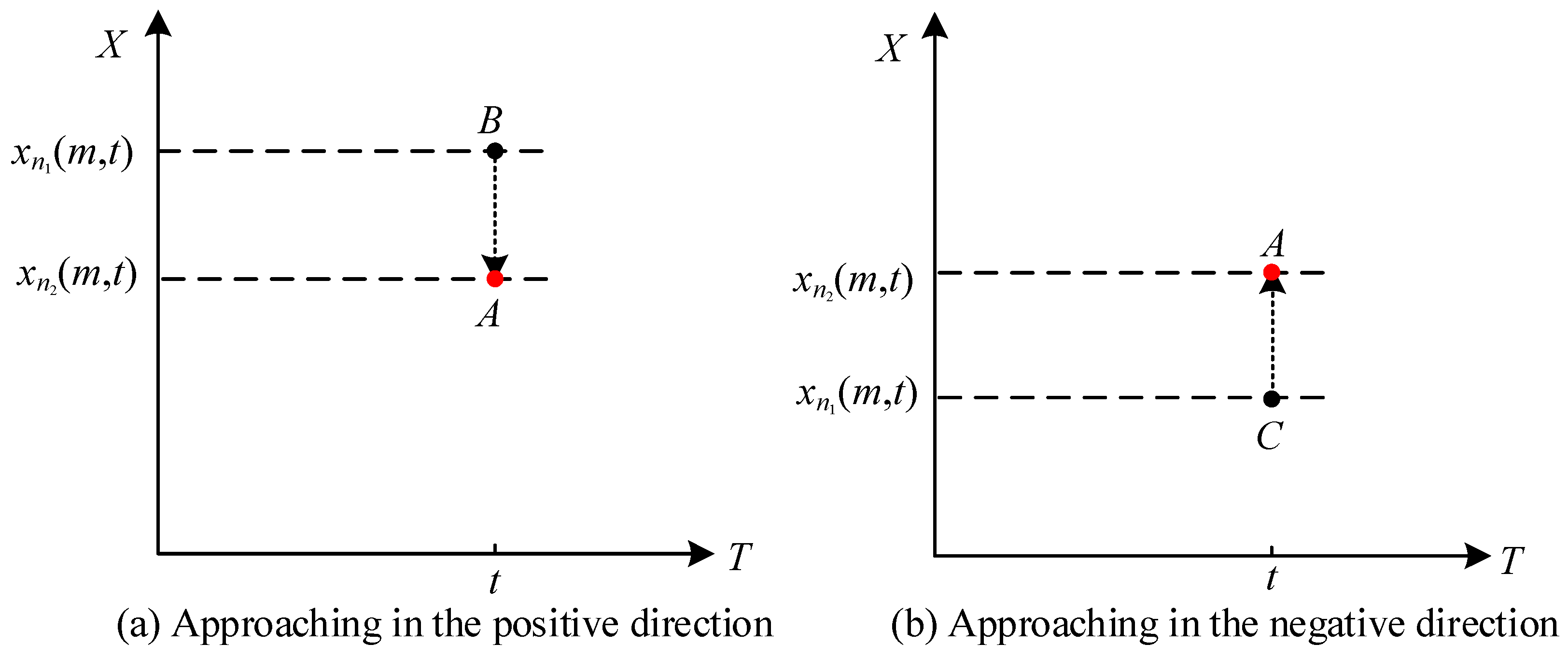The corresponding indicator value of $n_1$ about the object m is not less than or is less than the index value of $n_2$ at time t. The two cases are shown in Figure 1. In terms of nearness direction judgement, the index value of $n_2$ is taken as reference, so Figure 1a,b indicate that the index value of $n_1$ approaches the index value of $n_2$ about the mth object at time t in different directions.

The following will mainly introduce the preparation work for proposing the NGIM model.

Definition 3. 

Let ${\Delta }_{n_1,n_2}(m,t)=x_{n_1}(m,t)-x_{n_2}(m,t)$ and $\left|{\Delta }_{n_1,n_2}\right(m,t\left)\right|=|-{\Delta }_{n_2,n_1}(m,t\left)\right|=\left|x_{n_1}\right(m,t)-x_{n_2}(m,t\left)\right|$ be the directed distance and absolute distance of the indicator $n_1$ to $n_2$ $(n_1,n_2\in \{1,2,\cdots ,N\left\}\right)$ about the mth $(m\in \{1,2,\cdots ,M\left\}\right)$ object at time t $(t\in \{1,2,\cdots ,T\left\}\right)$, respectively. Then, ${\Delta }_{n_1,n_2}\left(m\right)=({\Delta }_{n_1,n_2}\left(m,1\right),{\Delta }_{n_1,n_2}\left(m,2\right),\cdots ,{\Delta }_{n_1,n_2}(m,T\left)\right)$ and $\left|{\Delta }_{n_1,n_2}\right(m\left)\right|=(\left|{\Delta }_{n_1,n_2}\left(m,1\right)\right|,\left|{\Delta }_{n_1,n_2}\left(m,2\right)\right|,\cdots ,|{\Delta }_{n_1,n_2}(m,T)\left|\right)$ are the time series of the directed distance and absolute distance sequence of the indicator $n_1$ to $n_2$ about the mth object, respectively.

Similarly, ${\Delta }_{n_1,n_2}\left(t\right)=({\Delta }_{n_1,n_2}\left(1,t\right),{\Delta }_{n_1,n_2}\left(2,t\right),\cdots ,{\Delta }_{n_1,n_2}(M,t\left)\right)$ and $\left|{\Delta }_{n_1,n_2}\right(t\left)\right|=(\left|{\Delta }_{n_1,n_2}\left(1,t\right)\right|,\left|{\Delta }_{n_1,n_2}\left(2,t\right)\right|,\cdots ,|{\Delta }_{n_1,n_2}(M,t)\left|\right)$ are the cross-sectional data of the directed distance and absolute distance sequence of the indicator $n_1$ to $n_2$ at time t, respectively.

The directionality of approach is considered in Definition 3; therefore ${\Delta }_{n_1,n_2}(m,t)=-{\Delta }_{n_2,n_1}(m,t)$, and $\left|{\Delta }_{n_1,n_2}\right(m,t\left)\right|=|-{\Delta }_{n_2,n_1}(m,t\left)\right|=\left|x_{n_1}\right(m,t)-x_{n_2}(m,t\left)\right|$.

In this paper, the degree of nearness is judged by absolute distance, and the direction of nearness is judged according to whether the indicator value is less than or no less than the reference value.

If the index value is no less than the reference value, the direction of nearness is positive; if the index value is less than the reference value, the direction of nearness is negative. Nearness direction judgement is defined as Definition 4.

Definition 4. 

Take $x_{n_2}(m,t)$ as the reference value; $T_{n_1,n_2}\left(m,t\right)=1$ indicates that the indicator value $n_1$ of the mth object is no less than that of $n_2$ at time t, and $T_{n_1,n_2}\left(m,t\right)=-1$ indicates that the indicator value $n_1$ of the mth object is less than that of $n_2$ at time t. Then, $T_{n_1,n_2}(m,t)=\{\begin{array}{c}1,{ \Delta }_{n_1,n_2}(m,t)\ge 0\\ -1, {\Delta }_{n_1,n_2}\left(m,t\right)<0\end{array}$ can be used to represent the direction of nearness of the indicator values $n_1$ to $n_2$ of the object m at time t. $T_{n_1,n_2}(m,t)$ is called the nearness direction judgement factor.

2.3. Formulae for Calculating the Nearness Grey Incidence Model

Based on the analysis of the nearness feature representation of panel data, the grey incidence coefficients and grey incidence degrees are proposed in this section. In addition, to improve the resolution of the new model, which can magnify the difference in grey incidence degree, the natural logarithm is used to judge the magnitude of the grey incidence coefficients, as mentioned by Liu et al. [29]. Methods to improve the stable robustness of the grey incidence analysis, which was first proposed by Sun et al. [32], can still be adopted in the new model. It acquires grey incidence degree by calculating the magnitude and symbol of the grey incidence coefficients separately. The novel nearness grey incidence mode is put forward as follows.

Definition 5. 

${\Delta }_{n_1,n_2}(m,t)$ and $T_{n_1,n_2}(m,t)$ are defined in Definitions 3 and 4, respectively. The nearness grey incidence coefficient of the indicator $n_1$ to $n_2$ $(n_1,n_2\in \{1,2,\cdots ,N\left\}\right)$ of the object m $(m\in \{1,2,\cdots ,M\left\}\right)$ at time t $(t\in \{1,2,\cdots ,T\left\}\right)$ can be expressed as ${\gamma }_{n_1,n_2}(m,t)=T_{n_1,n_2}(m,t)\cdot e^{-a\cdot \left|{\Delta }_{n_1,n_2}\right(m,t\left)\right|}$, in which $T_{n_1,n_2}(m,t)$, $e^{-a\cdot \left|{\Delta }_{n_1,n_2}\right(m,t\left)\right|}$ and $\alpha (0<\alpha \le 2)$ are the nearness direction judgement factor, measurement factor and adjustment factor of the measurement factor, respectively.

The grey incidence coefficient serves as the intermediate step in the correlation analysis process. Ultimately, we use the grey incidence coefficient to synthesize grey incidence degree. Different from the previous grey incidence models, which obtained the grey incidence degree by the weighted average of grey incidence coefficients, the new model is based on the physical meaning of nearness, and it calculates the grey incidence degree sign by determining whether the sum of the directed distance is positive or negative. It is specifically defined as follows.

Definition 6 (The symbol determination of grey incidence degree).

${\Delta }_{n_1,n_2}(m,t)$ is defined in Definition 3. Then, the nearness direction judgement factor of the mth object of the indicator $n_1$ to $n_2$ is shown in Formula (1):

$$T_{n_1,n_2}(m)=\{\begin{array}{c}1, {\sum }_{t=1}^T{\Delta }_{n_1,n_2}(m,t)\ge 0\\ -1, {\sum }_{t=1}^T{\Delta }_{n_1,n_2}(m,t)<0\end{array}$$

(1)

Similarly, the nearness direction judgement factor of the indicator $n_1$ to $n_2$ at time t can be defined as Formula (2):

$$O_{n_1,n_2}(t)=\{\begin{array}{c}1, {\sum }_{m=1}^M{\Delta }_{n_1,n_2}(m,t)\ge 0\\ -1, {\sum }_{m=1}^M{\Delta }_{n_1,n_2}\left(m,t\right)<0\end{array}$$

(2)

The model can reflect the directionality of data nearness, and the grey incidence coefficients may be positive and negative. How to obtain the grey incidence degree according to grey incidence coefficients is the key to improving the stable robustness of the model. This paper deeply considers the influence of nearness direction on the results of the grey incidence degree, uses the variance of the directed distance sequence to characterize the volatility of the difference between the two series, and uses it to correct the final grey incidence degree, as shown in Definition 7.

Definition 7. 

${\Delta }_{n_1,n_2}(m,t)$, ${\gamma }_{n_1,n_2}(m,t)$, $T_{n_1,n_2}\left(m\right)$ and $O_{n_1,n_2}\left(t\right)$ are defined in Definitions 3, 5 and 6. Let ${\gamma }_{n_1,n_2}^T(m)=T_{n_1,n_2}(m)\cdot {\displaystyle \frac{{\sum }_{t=1}^T\left|{\gamma }_{n_1,n_2}\right(m,t\left)\right|}{T}}\cdot e^{-\beta \cdot \sigma \left({\Delta }_{n_1,n_2}\right(m\left)\right)}$ and ${\gamma }_{n_1,n_2}^O\left(t\right)=O_{n_1,n_2}\left(t\right)\cdot Let{\displaystyle \frac{{\sum }_{m=1}^M\left|{\gamma }_{n_1,n_2}\right(m,t\left)\right|}{M}}\cdot e^{-\beta \cdot \sigma \left({\Delta }_{n_1,n_2}\right(t\left)\right)}$ be the nearness grey incidence sub-degree of panel data in the time dimension and object dimension, respectively. Here, $\sigma \left({\Delta }_{n_1,n_2}\right(m\left)\right)$ and $\sigma \left({\Delta }_{n_1,n_2}\right(t\left)\right)$ are the variance of directed distance sequences ${\Delta }_{n_1,n_2}\left(m\right)$ and ${\Delta }_{n_1,n_2}\left(t\right)$, respectively, and $\beta (0<\beta \le 2)$ is the adjustment factor of $\Delta$. The larger the variance value is, the more volatile the sequence is. $e^{-\beta \cdot \sigma \left({\Delta }_{n_1,n_2}\right(m\left)\right)}$ and $e^{-\beta \cdot \sigma \left({\Delta }_{n_1,n_2}\right(t\left)\right)}$ are the subtractive functions of $\sigma \left({\Delta }_{n_1,n_2}\right(m\left)\right)$ and $\sigma \left({\Delta }_{n_1,n_2}\right(t\left)\right)$ respectively, that is, the larger the fluctuation ( $\sigma$) is, the smaller the value of $e^{-\sigma }$ will be. Therefore, $e^{-\beta \cdot \sigma \left({\Delta }_{n_1,n_2}\right(m\left)\right)}$ and $e^{-\beta \cdot \sigma \left({\Delta }_{n_1,n_2}\right(t\left)\right)}$ are called the anti-fluctuation factors of panel data in the time dimension and object dimension, respectively.

In this paper, the anti-fluctuation factors are used to measure the influence of relative fluctuation between sequences on the calculation result of the nearness grey incidence degree.

Definition 8. 

Let $T_{n_1,n_2}$ be the nearness direction judgement factor of the two indicators $n_1$ and $n_2$ in the time dimension and object dimension, and the formula is as Formula (3).

$$T_{n_1,n_2}=\{\begin{array}{c}1, {\sum }_{m=1}^M{\sum }_{t=1}^T{\Delta }_{n_1,n_2}(m,t)\ge 0\\ -1, {\sum }_{m=1}^M{\sum }_{t=1}^T{\Delta }_{n_1,n_2}(m,t)<0\end{array}$$

(3)

Actually, considering the nearness direction between the two-panel data, whether the judgement factor is calculated from the time dimension or the space dimension is the same result, that is, $T_{n_1,n_2}$ can represent the nearness direction judgement factor in the time dimension, object dimension and panel data.

Then, the nearness grey incidence degree of panel data in the time dimension and object dimension are defined as ${\gamma }_{n_1,n_2}^T=T_{n_1,n_2}\cdot {\displaystyle \frac{{\sum }_{m=1}^M{\sum }_{t=1}^T\left|{\gamma }_{n_1,n_2}^T\right(m\left)\right|}{M\cdot T}}$ and ${\gamma }_{n_1,n_2}^O=T_{n_1,n_2}\cdot {\displaystyle \frac{{\sum }_{m=1}^M{\sum }_{t=1}^T\left|{\gamma }_{n_1,n_2}^O\right(m\left)\right|}{M\cdot T}}$, respectively.

Definition 9. 

The comprehensive nearness grey incidence degree of panel data is denoted as Formula (4):

$${\varphi }_{n_1,n_2}=T_{n_1,n_2}\cdot ({\omega }_T\cdot |{\gamma }_{n_1,n_2}^T|+{\omega }_O\cdot |{\gamma }_{n_1,n_2}^O\left|\right)$$

(4)

where $T_{n_1,n_2}$ and ${\omega }_T\cdot \left|{\gamma }_{n_1,n_2}^T\right|+{\omega }_O\cdot \left|{\gamma }_{n_1,n_2}^O\right|$ are the nearness direction judgement factor and measurement factor of panel data for the indiactors $n_1$ to $n_2$, respectively. ${\omega }_T\cdot \left|{\gamma }_{n_1,n_2}^T\right|+{\omega }_O\cdot \left|{\gamma }_{n_1,n_2}^O\right|$ is also used to calculate the absolute nearness grey incidence degree. $\left|{\gamma }_{n_1,n_2}^T\right|$ and $\left|{\gamma }_{n_1,n_2}^O\right|$ are the absolute value of the nearness grey incidence degree in the time dimension and object dimension, respectively. ${\omega }_T$ and ${\omega }_O$ are the weights of panel data in the time and object dimensions, respectively. In general, ${\omega }_T,{\omega }_O\in [0, 1]$, ${\omega }_T+{\omega }_O=1$, and the decision-maker can determine the values of ${\omega }_T$ and ${\omega }_O$ according to their importance.

2.4. Properties of the Nearness Grey Incidence Model

As shown in the aforementioned formulae and the model building process, the new model has its characteristics compared with the existing grey incidence models which can apply to a variety of data types, such as time-series data, cross-sectional data, panel data, and so on. There are six properties of the proposed model presented in this section, and the explanations of each property are given.

For the next six properties, recall that $X_n$ denotes the panel data matrix. Whether it is in the time dimension or object dimension, let $\Delta$ represents the directed distance of the observation value and $T$ or $O$ denote the nearness direction judgement factors in the time dimension or object dimension. In addition, $\gamma$ and $\varphi$ are referred to as the grey incidence coefficient and the grey incidence degree, respectively.

Property 1. 

(1) 

${\gamma }_{n_1,n_2}(m,t)\in (-1,0)\cup (0,1]$;

(2) 

${\gamma }_{n_1,n_2}^T\left(m\right)\in (-1,0)\cup (0,1]$, ${\gamma }_{n_1,n_2}^O\left(t\right)\in (-1,0)\cup (0,1]$;

(3) 

${\gamma }_{n_1,n_2}\left(m,t\right)=1\iff x_{n_1}(m,t)=x_{n_2}(m,t)$; ${\gamma }_{n_1,n_2}^T\left(m\right)=1, {\gamma }_{n_1,n_2}^O\left(t\right)=1\iff X_{n_1}=X_{n_2}$.

Proof. 

(1)

Since $\left|{\Delta }_{n_1,n_2}\right(m,t\left)\right|\in [0,+\mathrm{\infty })$, when $T_{n_1,n_2}(m,t)=1$, then ${\gamma }_{n_1,n_2}(m,t)\in (0,1]$; when $T_{n_1,n_2}\left(m,t\right)=-1$, then ${\gamma }_{n_1,n_2}(m,t)\in [-1,0)$. Both ${\gamma }_{n_1,n_2}\left(m,t\right)=1$ and ${\gamma }_{n_1,n_2}\left(m,t\right)=-1$ indicate that the two points coincide, so only one case is taken, ${\gamma }_{n_1,n_2}\left(m,t\right)=1$.

(2)

According to (1) and Definition 7, there is ${\gamma }_{n_1,n_2}^T\left(m\right)\in (-1,0)\cup \left(0,1\right]$.

(3)

It is easy to prove that the nearness grey incidence degree is equal to 1 if and only if the two values are the same. □

Property 2. 

The order of objects does not affect the nearness grey incidence degree and the ranking of grey incidence degree.

Since the calculation process does not involve the distance between objects, the calculation result of the nearness grey incidence degree is not affected by the order of object dimension.

Property 3. 

The model applies to time series, cross-sectional data and panel data.

The nearness grey incidence model, which has been constructed in Section 2.2 and Section 2.3, is based on panel data, while time series and cross-sectional data are special cases of panel data, so the new model is also applicable to time series and cross-sectional data.

Property 4. 

The new model satisfies uniqueness, comparability and antisymmetry.

The unique nearness grey incidence coefficients and nearness grey incidence degrees will be produced according to the input values. Then, the calculation result meets uniqueness.

The nearness grey incidence coefficients and nearness grey incidence degrees are unique. Therefore, the results of the model are comparable.

Since the model considers the direction of data nearness, the nearness grey incidence coefficient between $x_{n_1}(m,t)$ and $x_{n_2}(m,t)$ and the nearness grey incidence coefficient between $x_{n_2}(m,t)$ and $x_{n_1}(m,t)$ are the negative of each other. In other words, ${\gamma }_{n_1,n_2}\left(m,t\right)=-{\gamma }_{n_2,n_1}(m,t)$.

Property 5. 

The relative fluctuation of data will affect the nearness grey incidence degree.

The relative fluctuation of the sequence will affect the variance of the difference sequence; the larger the fluctuation of the sequence is, the larger variance ($\sigma$) will be. Since $0<\beta \le 1$, $e^{-\beta \cdot \sigma \left({\Delta }_{n_1,n_2}\right(m\left)\right)}$ and $e^{-\beta \cdot \sigma \left({\Delta }_{n_1,n_2}\right(t\left)\right)}$ are the subtractive functions of $\sigma \left({\Delta }_{n_1,n_2}\right(m\left)\right)$ and $\sigma \left({\Delta }_{n_1,n_2}\right(t\left)\right)$, respectively, the relative fluctuation between sequences will reduce the nearness grey incidence degree to a certain extent.

Property 6. 

The model applies to the measurement of nearness grey incidence degree between any two objects.

The model building process in Section 2.2 and Section 2.3 only introduces the nearness grey incidence degree of panel data for any two indicators. Actually, as long as the data have comparable practical meaning, it is also suitable to determine how close the data are between any two objects.

3. Case Study

According to the Ambient Air Quality Standards (GB3095-2012) [33], which was implemented nationwide in 2016, there are six basic environmental pollutants: PM_2.5 (particulate matter with an aerodynamic diameter less than 2.5 mm), PM₁₀ (particulate matter with an aerodynamic diameter less than 10 mm), SO₂ (sulfur dioxide), CO (carbon monoxide), NO₂ (nitrogen dioxide), and O₃ (ozone). In addition, the quality of air is reflected by AQI (air quality index).

Next, we will analyze the distribution characteristics of the six different pollutants in the Beijing–Tianjin–Hebei region from 2016 to 2024 according to the monthly data calculated from the daily concentration of six pollutants, and also analyze the overall environmental pollution situation according to AQI.

In Section 3.1, the original data sources and how to obtain the monthly data with daily data are described. The NGIM is utilized to analyze the distribution characteristics of each pollutant in Section 3.2. To highlight the advantages of the model in nearness judgement and panel data analysis, in Section 3.3, systematic comparisons are compared with a series of traditional grey incidence models.

3.1. Data Source

Six pollutants (SO₂, PM_2.5, PM₁₀, O₃, NO₂ and CO) are determined to analyze the distribution characteristics of different indexes in BTH, which contains 13 cities (Beijing, Tianjin, Shijiazhuang, Tangshan, Qinhuangdao, Handan, Baoding, Zhangjiakou, Chengde, Cangzhou, Langfang, Hengshui, Xingtai). The daily data of the six indicators of the 13 cities from 1 January 2016 to 31 December 2024 are acquired from the China Air Quality Online Monitoring and Analysis Platform, whose website is https://www.aqistudy.cn/historydata/, accessed on 1 March 2026. In addition, we used the linear interpolation method to fill in the missing data.

In this paper, monthly pollutant concentrations were used to analyze the main pollutants and their distribution in BTH. However, there is a mismatch between monthly AQI acquisition and pollutant concentration on the website. For example, the ozone concentration data collected from the website are all 8 h moving average concentrations, while the individual air quality indexes (IAQI) of ozone should be calculated by 1 h average concentration according to the Ambient Air Quality Index Technical Regulations, which was promulgated by the Ministry of Environmental Protection of the People’s Republic of China. Moreover, the monthly AQI is obtained by averaging the daily AQI, which takes the maximum daily IAQI among all pollutants. Therefore, even if the ozone 8 h moving average concentration is converted into AQI, the AQI published on the website cannot be correlated with the AQI corresponding to ozone. We cannot calculate the nearness grey incidence degree using the AQI calculated by the 1 h concentration of ozone with the AQI calculated by the 8 h concentration, as there is a clear mismatch between them.

To solve this question, according to the technical regulations for environmental air quality index (AQI) (HJ 633—2012), we use the collected daily pollutant concentration data to acquire the IAQI, and the daily AQI is the maximum value of the daily IAQI of different pollutants. Then, the monthly comprehensive AQI is the average value of the daily AQI, represented by the following formulae.

$$AQI{\left(q\right)}_{daily}=\mathrm{m}\mathrm{a}\mathrm{x}\left\{IAQI\right(1,q),IAQI(2,q),\cdots ,IAQI(p,q),\cdots ,IAQI(P,q\left)\right\},$$

where p is the number of pollutants, and q is the daily time number.

$$AQI{\left(p\right)}_{monthly}={\sum }_{q=1}^{Q}IAQI(p,q),$$

Q is the number of days in the month, and $AQI{\left(p\right)}_{monthly}$ is the mean value of the daily IAQI of the pth pollutant in a certain month.

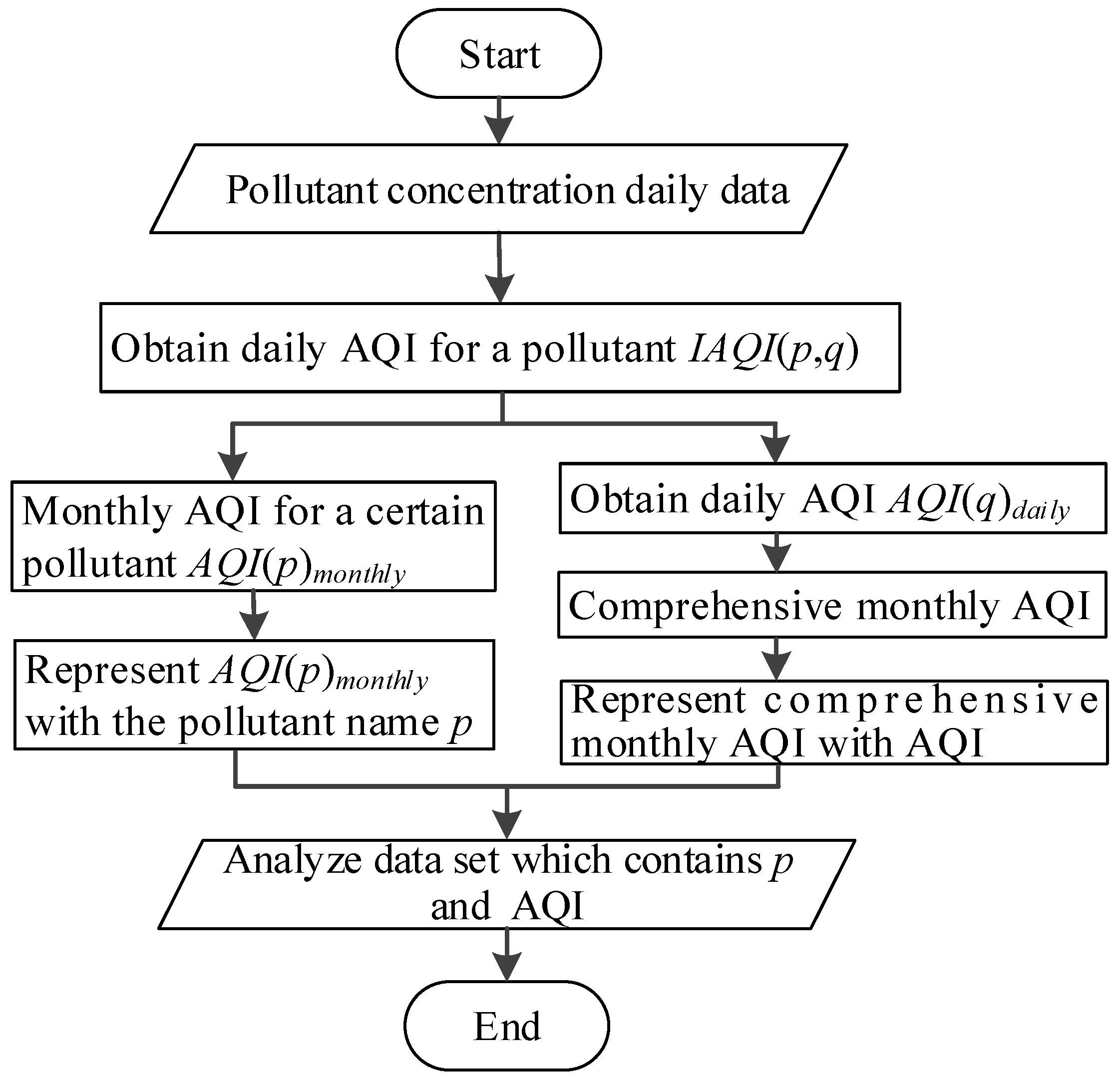
The flow chart of the acquisition of the calculation data set is shown in Figure 2. The pseudo-code for data standardization is shown in Algorithm 1.

Algorithm 1. Standardized data acquisition

Data: Original daily data of six pollutants from 2016 to 2024

Result: Standardized data

1. Load original data;

2. Linear interpolation method fills in the missing values;

3. Calculate IAQI based on Table 3. Table IAQI and corresponding pollutant concentration limits. IAQI Pollution Concentration Limits SO2 /(μg/m3) NO2 /(μg/m3) CO /(mg/m3) O3 /(μg/m3) PM10 /(μg/m3) PM2.5 /(μg/m3) 0 0 0 0 0 0 0 50 50 40 2 100 50 35 100 150 80 4 160 150 75 150 475 180 14 215 250 115 200 800 280 24 265 350 150 300 1600 565 36 800 420 250 400 2100 750 48 * 420 350 500 2620 940 60 * 600 500 * indicates that the value is null. When the O3 8 h average concentration value is higher than 800 μg/m3, the IAQI will not be calculated. In this paper, there is no O3 concentration beyond this range. ;

4. Synthetic monthly AQI for every pollutant according to the results of Step 3.

5. Obtain daily AQI;

6. Synthetic daily AQI according to the results of Step 4;

7. Standardize each indicator;

8. Save standardized data.

Using the calculated various types of AQIs, the main analysis is as follows: by calculating the grey incidence degree between the monthly comprehensive AQI and the monthly AQI of different pollutants, the major pollutants and their temporal and spatial distribution can be distinguished; by comparing the grey incidence degree between the monthly AQIs of a certain pollutant at two times, the pollution of the pollutant at different times can be analyzed; by calculating the grey incidence degree between the monthly AQIs of a pollutant in different cities, the pollution situation of the pollutant in the two cities can be compared and analyzed.

In addition, the individual air quality indexes, abbreviated as IAQI, are calculated according to the next formula.

$$IAQ{I}_P={\displaystyle \frac{IAQ{I}_{Hi}-IAQ{I}_{Lo}}{B{P}_{Hi}-B{P}_{Lo}}}(C_P-B{P}_{Lo})+IAQ{I}_{Lo}$$

where $IAQ{I}_P$ is the IAQI of pollutant p; $C_P$ represents the concentration value of pollutant p; $B{P}_{Hi}$ and $B{P}_{Lo}$ can be considered as the high and low value of pollutant concentration limits similar to $C_P$ in Table 3, respectively. $IAQ{I}_{Hi}$ and $IAQ{I}_{Lo}$ are the IAQI of $B{P}_{Hi}$ and $B{P}_{Lo}$, respectively.

For simplicity, abbreviations of cities are used to represent the names of different cities. For example, we label Beijing as BJ, and other cities use the same naming principle. The full names and abbreviations of other cities are as follows: Tianjin—TJ, Shijiazhuang—SJZ, Tangshan—TS, Qinhuangdao—QHD, Handan—HD, Xingtai—XT, Zhangjiakou—ZJK, Chengde—CD, Cangzhou—CZ, Langfang—LF, Hengshui—HS, Baoding—BD.

3.2. Model Calculation and Analysis

In this section, according to different systems as benchmarks, the NGIM is utilized to analyze the different characteristics of pollutants in BTH from 2016 to 2024. This part is mainly divided into several subsections: Firstly, to obtain the major pollutants in BTH, the proposed model is used to calculate the grey incidence degree between the monthly AQI of each pollutant and monthly comprehensive AQI in Section 3.2.1. Subsequently, we analyze the spatiotemporal distribution characteristics of pollutants by analyzing the grey incidence sub-degree and grey incidence coefficients, which are presented in Section 3.2.2. In Section 3.2.3, by analyzing the grey incidence degree between the year-by-year data and the data in 2024, the changing trend of major pollutants in BTH from 2016 to 2024 was obtained. Finally, in Section 3.2.4, based on Beijing pollutant data, the similarities and differences of pollution between different cities and Beijing are analyzed. It is worth emphasizing that all data in this section are standardized.

3.2.1. Identification of Major Pollutants

This part mainly introduces the grey incidence degrees between different monthly pollutants’ AQI and the comprehensive monthly AQI, which has been shown in

Table 4. The NGIDs between different pollutants and AQI.

Indicators	${\mathit{\gamma }}_{\mathit{n}}^{\mathit{T}}$	$\mathbf{ABS} {\mathit{\gamma }}_{\mathit{n}}^{\mathit{T}}$	Rank	${\mathit{\gamma }}_{\mathit{n}}^{\mathit{O}}$	$\mathbf{ABS} {\mathit{\gamma }}_{\mathit{n}}^{\mathit{O}}$	Rank	${\mathit{\varphi }}_{\mathit{n}}$	$\mathbf{ABS} {\mathit{\varphi }}_{\mathit{n}}$	Rank
SO2-AQI	−0.2584	0.2584	6	−0.2795	0.2795	6	−0.2689	0.2689	6
PM2.5-AQI	−0.5207	0.5207	2	−0.6508	0.6508	1	−0.5857	0.5857	2
PM10-AQI	−0.5676	0.5676	1	−0.6490	0.6490	2	−0.6083	0.6083	1
O3-AQI	−0.4263	0.4263	3	−0.6192	0.6192	3	−0.5228	0.5228	3
NO2-AQI	−0.3884	0.3884	4	−0.4445	0.4445	4	−0.4164	0.4164	4
CO-AQI	−0.2943	0.2943	5	−0.3172	0.3172	5	−0.3057	0.3057	5

. For convenience, different monthly pollutants’ AQI and the comprehensive monthly AQI are replaced by pollutant names and AQI respectively. Within Table 4, the first column represents the combinations of different pollutants with the comprehensive monthly AQI. The arrays of the grey incidence degree between AQI and its related indicators are given in the second, fourth and sixth columns in Table 4, and represent the grey incidence degree in the time dimension, object dimension and comprehensive grey incidence degree, represented by ${\gamma }_n^T$, ${\gamma }_n^O$ and ${\varphi }_n$, respectively. In addition, the remaining columns are absolute values of the corresponding grey incidence degree. ABS in the table is the abbreviation of “absolute”. The rank is the ordering of the absolute value of the corresponding grey incidence degree. For simplicity, the nearness grey incidence degrees are marked as NGIDs.

As shown in Table 4, regardless of whether the NGIDs are in the time dimension (${\gamma }_n^T$), the object dimension (${\gamma }_n^O$), or comprehensive dimension (${\varphi }_n$), they are all negative numbers. This means that all pollutants are calculated from the NGIDs from the direction of the overall-less-than AQI. Similar conclusions can be drawn from the way of obtaining the comprehensive monthly AQI, which is the mean of daily AQI, and daily AQI is the maximum of six pollutants’ daily IAQI. This results in a monthly AQI for all pollutants less than the comprehensive monthly AQI. After determining the direction of the nearness grey incidence degree, the degree of each pollutant to the AQI should be judged from the numerical value of the NGIDs, that is, its absolute value. The higher the absolute value, the higher the nearness, and the higher the level of pollution.

The top three in the absolute values of comprehensive NGIDs are PM₁₀, PM_2.5 and O₃, which means, from the perspective of the time dimension and object dimension of panel data, PM₁₀, PM_2.5 and O₃ are the main pollutants in BTH from 2016 to 2024. There are different NGIDs rankings in different dimensions. From the time dimension, the top three combinations in the absolute value of NGIDs are AQI-PM₁₀, AQI-PM_2.5, and AQI-O₃, while the top three combinations in the object dimension are AQI-PM_2.5, AQI-PM₁₀, and AQI-O₃. This indicates that there are differences in the data volatility of panel data in the time dimension and the object dimension. The impact of the volatility between series on the calculation results of the NGID will be introduced in detail in Section 3.3.2. As to the remaining three pollutants NO₂, SO₂ and CO, it is obvious that the ranking of the NGIDs of NO₂-AQI, SO₂-AQI and CO-AQI does not differ due to different computational dimensions, and the absolute values of NGIDs are low, indicating that the three pollutants have a low degree of nearness with AQI. Then, from an overall view, compared with other pollutants, NO₂, SO₂ and CO are not the major pollutants.

3.2.2. Spatiotemporal Distribution of Different Pollutants

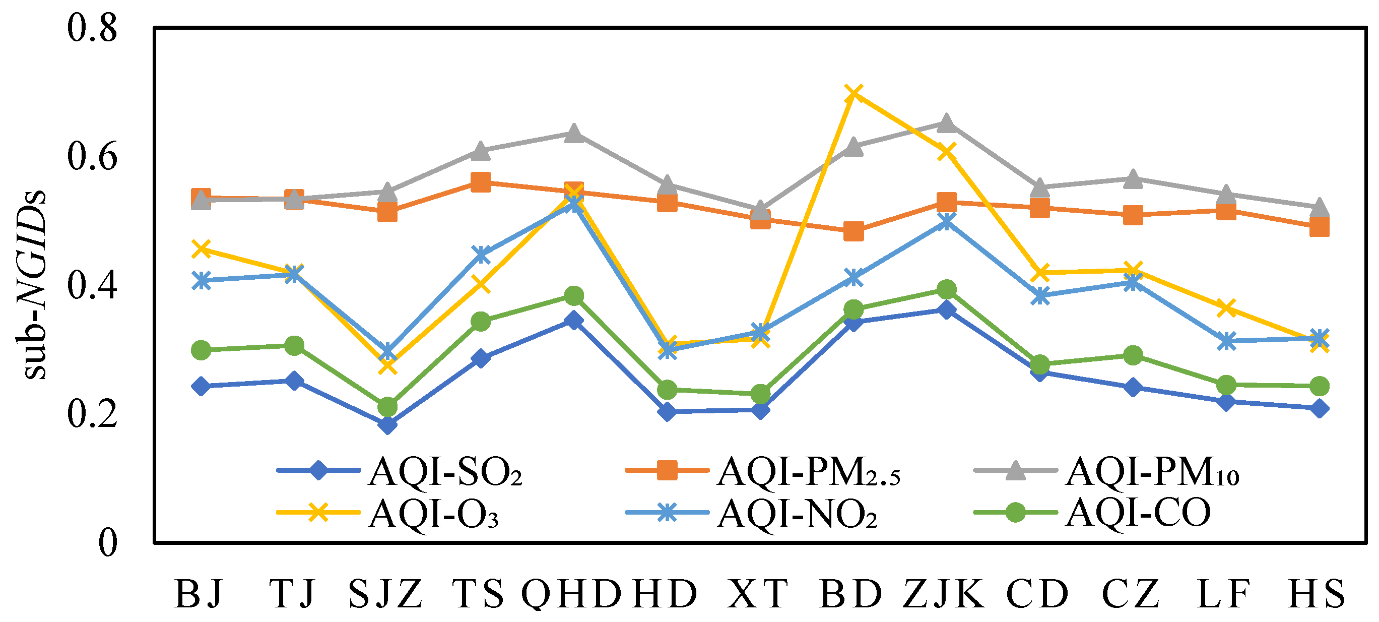
To more clearly show the pollutants in different regions and different periods, this part will analyze the nearness grey incidence sub-degrees (sub-NGIDs) and grey incidence coefficients of the time and object dimensions. It can be seen from the time dimension NGIDs’ diagram, which is depicted in Figure 3, that the absolute values of sub-NGIDs between PM_2.5, PM₁₀ and AQI in different regions has always been ranked high; the pollution severity of SO₂ and CO has always been at a low level. Comparatively speaking, the pollution level of CO is slightly higher than that of SO₂; the pollution severity of NO₂ and O₃ in different regions varies greatly, and the absolute values of the sub-NGIDs are in the middle level, lower than PM_2.5, PM₁₀, and higher than SO₂ and CO.

By evaluating the absolute grey incidence sub-degrees in the time dimension, the main pollutants vary in different regions, but mainly are PM_2.5 PM₁₀ and O₃, as presented in Figure 3. Apart from BD and ZJK, the top two pollutants in other cities are PM_2.5 and PM₁₀. The pollution of O₃ is quite severe in both BD and ZJK. Except for PM_2.5, PM₁₀ and O₃, NO₂ has a higher grey incidence degree with AQI. NO₂ is in the third position in TJ, SJZ, TS, XT and HS. As we can see from Figure 3, compared with NO₂, the grey incidence degree of O₃ in different regions fluctuates significantly. Similar to the results of the grey incidence degree analysis in Section 3.2.1, the grey incidence sub-degrees between CO, SO₂ and AQI are at a low level compared with the other four pollutants.

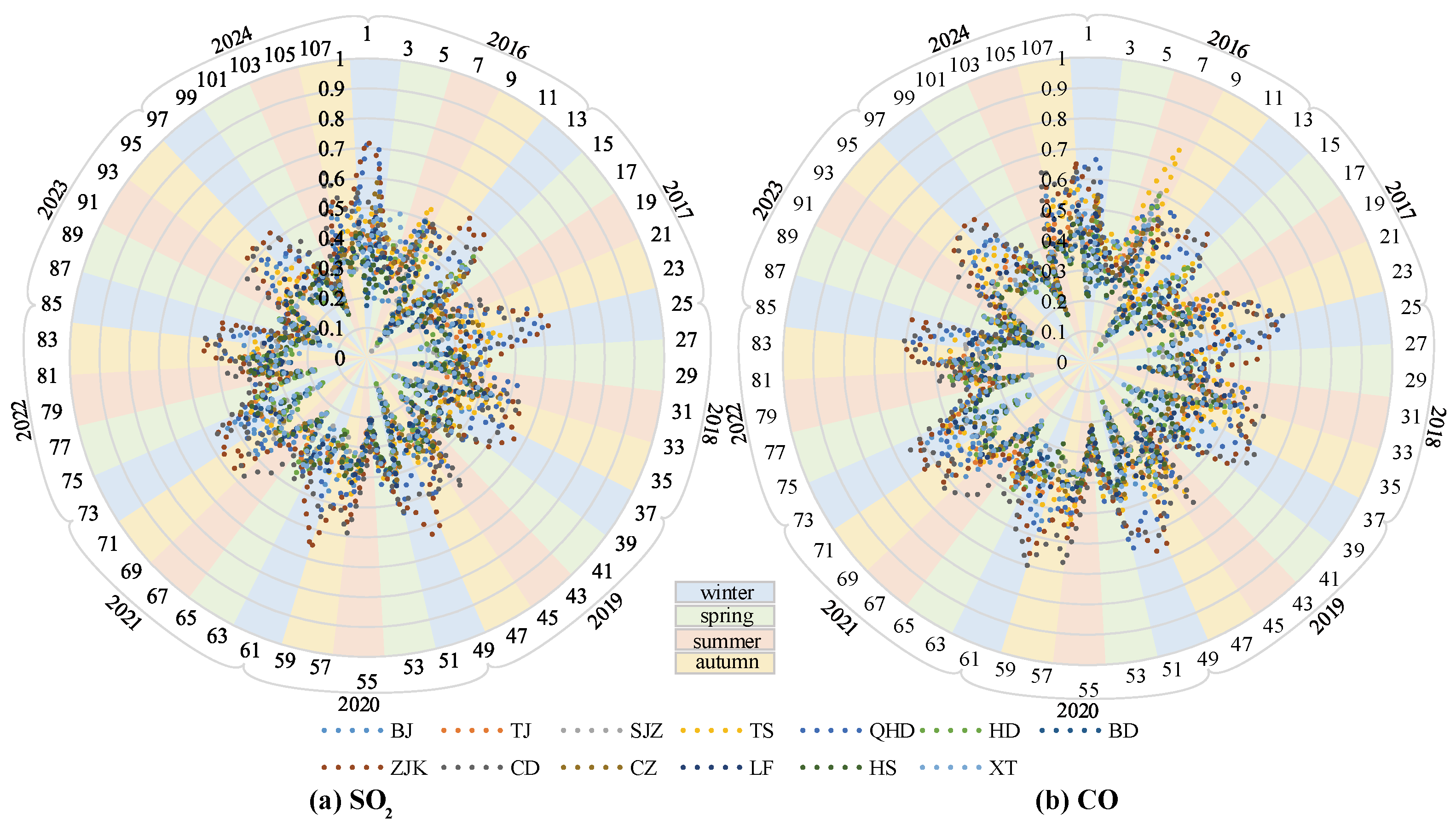
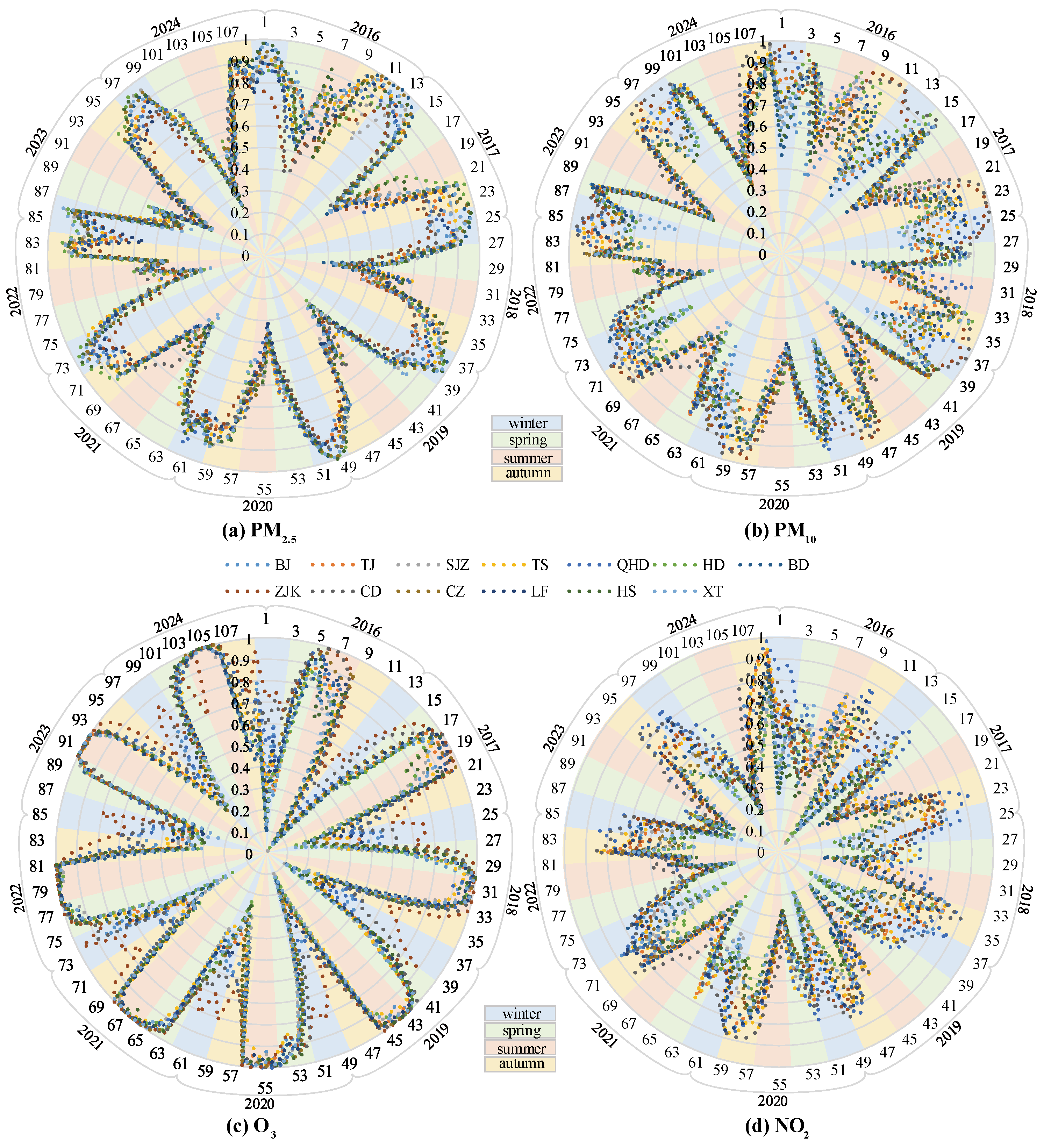
The absolute values of the grey incidence coefficient of different pollutants in the time dimension will be analyzed in detail below to reveal the seasonal characteristics of different pollutants. The grey incidence coefficients of different pollutants are shown in Figure 4 and Figure 5. The axis of the radar chart represents the absolute value of the grey incidence coefficient. The numbers in the outermost circle indicate the month number of the research data, 2016–2024, a total of 9 years, and 108 months. The outermost 2016–2024 in each subgraph represents the years. Four shading colours, light blue, light green, light red and light yellow represent the four seasons of winter, spring, summer and autumn respectively. The 13 cities are represented by dotted lines in 13 colours. From Figure 4, each graph represents the grey incidence coefficients between a certain pollutant and AQI for all cities in 108 months. The final graphs are all flowers, but the shape and size of petals are different. The larger the petals, the larger the grey incidence coefficients in a certain period, and more petals there are, the shorter the duration of pollution each petal represents. In a general sense, when the grey incidence coefficient is greater than 0.9, the degree of nearness is considered to be extremely strong. Therefore, this paper takes 0.9 as the limit to judge the main pollution period of different pollutants.

First, we analyze the relatively serious pollution of PM_2.5, PM₁₀, O₃ and NO₂ among the six pollutants. From Figure 4 as a whole, the seasonal distribution characteristics of PM_2.5 and O₃ are particularly obvious for almost all cities; the seasonal characteristics of PM₁₀ and NO₂ are weaker than the former two, and the seasonal distribution characteristics of PM₁₀ in some cities are different from other cities. PM_2.5 and PM₁₀ show evolutionary pollution characteristics: From 2016, pollution may occur all year round, and in 2023 and 2024, pollution is more serious only in autumn and winter.

From the pollution characteristics of each pollutant, PM_2.5 pollution occurred in four seasons of the year in 2016–2018, but was concentrated in autumn and winter. The fluctuation of the grey incidence coefficients in Figure 4a clearly shows the fluctuation characteristics of PM_2.5 over time. From 2019 to 2024, the main period of PM_2.5 pollution is concentrated in autumn and winter. Furthermore, the PM_2.5 pollution period is gradually concentrated, and the grey incidence coefficient with AQI has a downward trend, because the size of the petal in Figure 4a has a decreasing trend, especially in 2020 and 2024.

The characteristics of O₃ pollution are more obvious, as shown in Figure 4c, mainly concentrated in summer, but also in some months of spring and autumn. This makes the O₃ pollution show a situation where the number of petals is large and the number of petals is relatively small, and the boundaries between petals are relatively clear. The level of O₃ pollution in CD and ZJK is more serious than in other cities. The specific performance is that the grey incidence coefficient between O₃ and AQI has been higher than 0.9 in the summer of 2016.

There are differences in PM₁₀ pollution characteristics in different cities, just as depicted in Figure 4b. As for CD and ZJK, the PM₁₀ pollution season evolved from autumn, winter and spring in 2016 and 2019 to PM₁₀ pollution concentrated in autumn and winter in 2020 and 2024. Therefore, the grey incidence coefficient graph between PM₁₀ and AQI of CD and ZJK shows that the petals are larger in the first four years, and the petals are narrower in the next five years. For cities other than CD and ZJK, from 2016, the PM₁₀ concentration has been high throughout every season of the year. From 2017 to 2019, the PM₁₀ pollution is more serious in spring, autumn and winter, and then in 2020 and 2024, the PM₁₀ pollution is mainly concentrated in autumn and winter. For all cities, from 2016 to 2024, PM₁₀ pollution experienced a change from pollution occurring in every season of a year to mainly concentrated in autumn and winter, indicating that the period of PM₁₀ pollution in a year is gradually shortened, and the pollution period is more concentrated.

In Figure 4d, only in QHD, the absolute value of the grey incidence coefficient between NO₂ and AQI was greater than 0.9 once each, and in all cities it was mainly concentrated between 0.6 and 0.9. NO₂ pollution occurs in every season of the year, but the main pollution periods are concentrated in autumn and winter. Compared with O₃ and PM_2.5, the seasonal characteristics of NO₂ pollution are not strong, and the pollution level is lower, which is evident from the size of the petals.

For two pollutants SO₂ and CO, it can be seen from the petal size in the radar chart in Figure 5 that there are also certain seasonal characteristics, but the overall pollution level is low. Only in the winter of 2016 did the grey incidence coefficient of QHD and SJZ exceed 0.6.

3.2.3. Judging the Development Trend of Air Pollution

Based on the last year in the research data range, in this article, 2024 data was selected as benchmark data; the NGIDs between different pollutants for 2016–2023 and 2024 can be analyzed, and then the overall pollution changes in different pollutants in the last 9 years can be judged. Row and column headings represent year and indicator, respectively. Therein, “2016–2024” refers to the indicator value in 2016 minus the indicator value corresponding to 2024; other row headings have similar meanings. The main part of the table indicates the NGIDs. Taking the SO₂ row as an example, 0.6323 is the NGID between the SO₂ monthly AQI in 2016 and the SO₂ monthly AQI in 2024. A positive NGID sign indicates that the SO₂ monthly AQI value in 2016 is higher than that in 2024, and it also reflects that the overall SO₂ pollution level in BTH in 2016 is more serious than that in 2024. It is worth noting that since the 2024 data is used as the benchmark, the NGIDs of all pollutants corresponding to 2024 in

Table 5. The NGIDs between different years of each pollutant and the indicator data in 2024.

Years Indicators	2016–2024	2017–2024	2018–2024	2019–2024	2020–2024	2021–2024	2022–2024	2023–2024	2024–2024
SO2	0.6323	0.6866	0.7876	0.8312	0.8792	0.9220	0.9394	0.9492	1.0000
PM2.5	0.4364	0.5093	0.6215	0.6574	0.6960	0.7459	−0.7426	0.7587	1.0000
PM10	0.5521	0.5931	0.7085	0.7131	0.7484	−0.8303	−0.7731	0.7279	1.0000
O3	−0.7456	0.7707	−0.8490	0.7806	−0.8458	−0.8076	−0.8065	0.8237	1.0000
NO2	0.6005	0.6240	0.7150	0.7364	0.7861	0.8412	0.8680	0.8361	1.0000
CO	0.6674	0.7056	0.8026	0.8184	0.8595	0.9088	0.9357	0.9400	1.0000

are 1.

As can be seen from Table 5, almost all nearness grey incidence sub-degrees (sub-NGIDs) are greater than 0. However, O₃ had negative sub-NGIDs in 2016, 2018, 2020, 2021, and 2022. PM₁₀ and PM_2.5 had negative sub-NGIDs in 2021 and 2022, respectively. Take O₃ as an example; a negative sign appears in the sub-NGIDs, indicating that the overall pollution of O₃ in 2016, 2018, 2020, 2021, and 2022 is lighter than that in 2024. This is because it calculates the sub-NGIDs from the direction in which the overall value is less than the O₃ indicator value in 2024. These changes in O₃ might be related to the El Niño phenomenon [34]. The absolute value of the sub-NGIDs indicates the degree of closeness. The closer the value is to 1, the higher the degree of closeness. Judging from the absolute value of sub-NGIDs between O₃ in 2018 and 2024, the value of 0.8490 is large, indicating that the degree of pollution deterioration of O₃ in 2018 and 2024 is not much different, and the overall degree of closeness between 2018 and 2024 is relatively high. The above analysis indicates that the pollution level of O₃ has significantly increased in recent years, especially in 2023 and 2024. This is in line with the research conclusions of many scholars [35]. For PM_2.5 and PM₁₀, it might be because during the pandemic [36], many factories temporarily suspended their operations, resulting in better conditions in 2021 and 2022 compared to 2024.

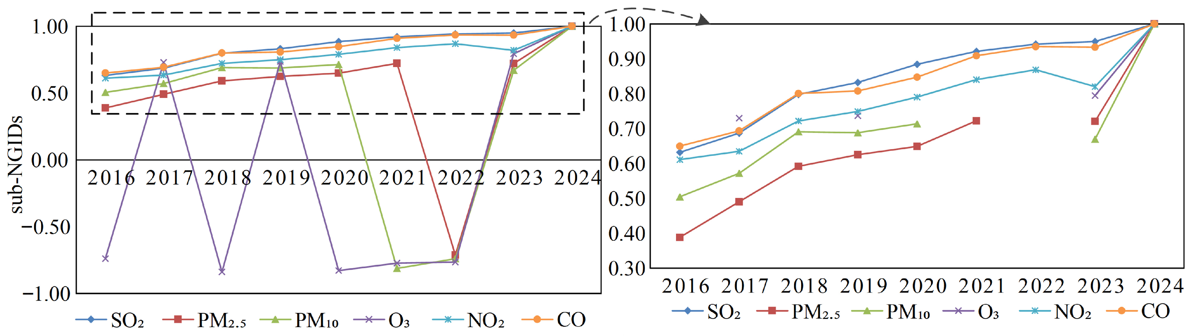
The sub-NGIDs of the other three pollutants, SO₂, NO₂ and CO, in 2016–2023 and 2024 are all positive numbers, indicating that these pollutants in 2016–2023 are all calculated from the overall values greater than 2024. The overall pollution level of pollutants in 2016–2023 is more serious than that in 2024. From the line chart in Figure 6, we can more clearly see the pollution change trend of various pollutants as a unit of one year. As can be seen from Figure 6, the sub-NGIDs between all pollutants except O₃, PM₁₀ and PM_2.5 in different years and 2024 show a monotonically increasing trend. As for positive sub-NGIDs, the smaller the value of the grey incidence sub-degrees, the greater the difference in serious pollution compared to 2024. Therefore, SO₂, NO₂ and CO are showing a trend of pollution improvement year by year, which can be seen more intuitively in the enlarged section in Figure 6. Among the three pollutants, the most obvious improvement is NO₂. The NGIDs have always been positive, and the sub-NGIDs have increased significantly from 2016 to 2024. SO₂ and CO improved to a lesser extent because they were less polluted in 2016, so there is not much room for improvement.

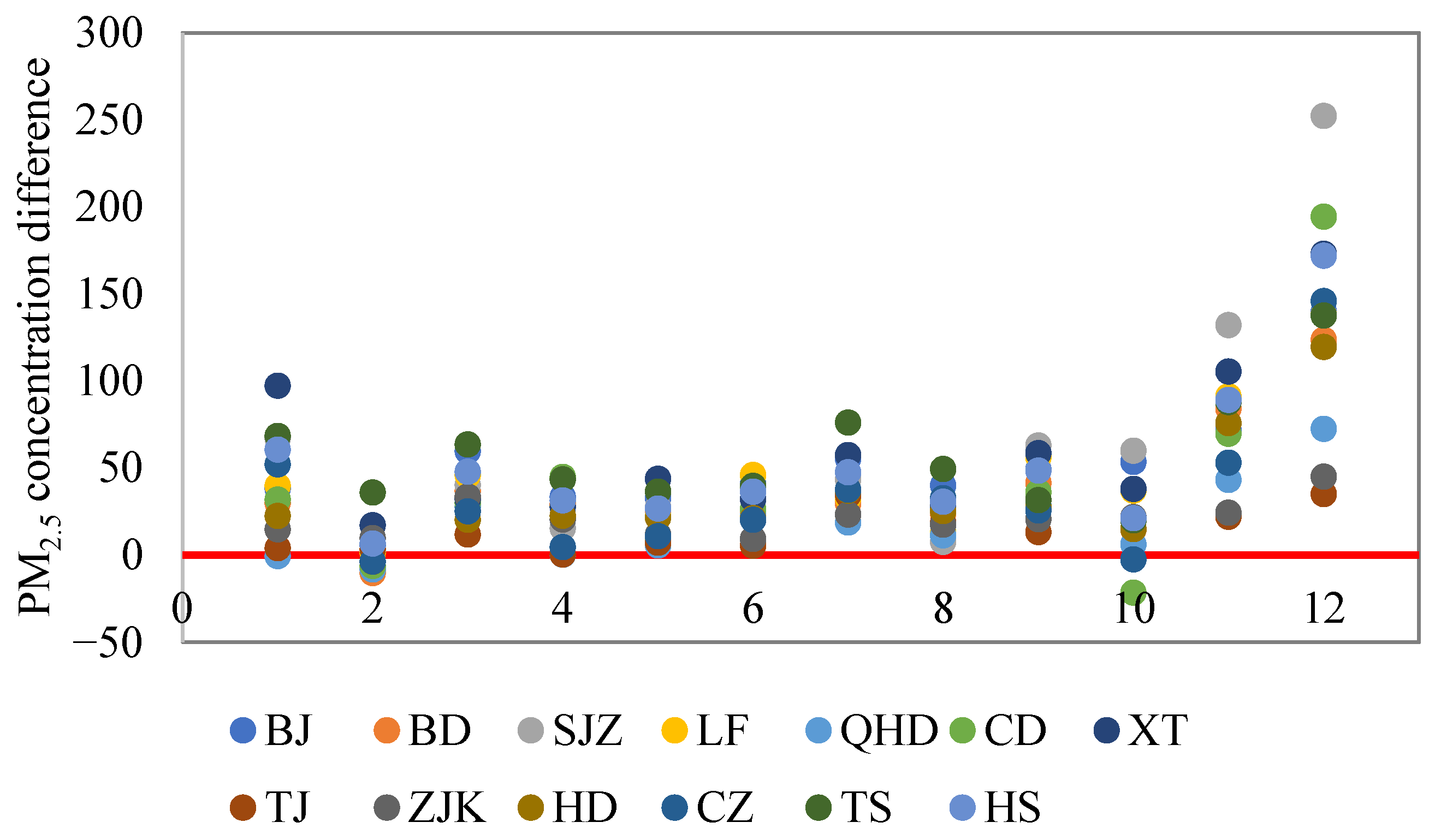
In order to explain the rationality of the model in this paper more intuitively, Figure 7 shows the scatter plot of the PM_2.5 difference between 2016 and 2024 in the BTH. Therein, the vertical axis represents the PM_2.5 difference between 2016 and 2024; to be precise, it is the indicator value in 2016 minus the indicator value in 2021, and the horizontal axis represents the 12 months of each year. In February, PM_2.5 in many cities in 2016 was lower than that in 2024. And except for February, PM_2.5 in almost all of the months in 2016 is higher than that in 2024. In January, November and December, the difference between PM_2.5 in 2016 and 2024 is larger. This shows that compared with 2016, the PM_2.5 concentration in these three months in 2024 declined more greatly. On the whole, most of the points are above the 0 scale, which verifies the fact that the PM_2.5 pollution situation in 2016 is more serious than that in 2024. The actual data has proved that the PM_2.5 pollution situation in 2024 was better than that in 2016.

3.2.4. Grey Incidence Analysis with Beijing as the Benchmark

In this subsection, Beijing, abbreviated as BJ, as China’s political centre, cultural centre, international exchange centre, and technology innovation centre, is the core city of BTH urban agglomeration. The following will calculate the NGIDs of some kind of pollutant between a certain city and BJ.

Table 6. The sub-NGIDs between cities in BTH and Beijing.

Indicators City Combinations	SO2	PM2.5	PM10	O3	NO2	CO
BJ-BJ	1.0000	1.0000	1.0000	1.0000	1.0000	1.0000
TJ-BJ	0.8786	0.7254	0.8166	0.8038	0.7882	0.8849
SJZ-BJ	0.7407	0.4830	0.5040	0.7564	0.7809	0.8262
TS-BJ	0.6914	0.7115	0.7164	0.8423	0.7504	0.7300
QHD-BJ	0.7848	−0.6870	0.8235	−0.7584	0.8384	0.8427
HD-BJ	0.7243	0.4697	0.5399	0.7394	0.7942	0.7844
BD-BJ	0.7629	0.5291	0.6202	0.7824	0.7522	0.8262
ZJK-BJ	0.8721	−0.5700	−0.8075	0.7572	−0.7017	−0.8634
CD-BJ	0.8656	−0.6217	−0.8384	−0.7841	−0.8108	0.8798
CZ-BJ	0.7553	0.6141	0.7319	0.7733	0.8097	0.8752
LF-BJ	0.9040	0.7260	0.7780	0.8590	0.8158	0.9096
HS-BJ	0.8165	0.5532	0.6463	0.7673	−0.7881	0.8797
XT-BJ	0.6956	0.5100	0.5824	0.7431	0.7813	0.7817

shows the NGIDs between cities in BTH and Beijing regarding certain pollutants. Row and column headings represent different pollutants and city combinations, respectively. It is possible to deeply analyze the impact of different pollutants in other cities in BTH and BJ.

According to different pollutants, from the SO₂ in the second column, the sub-NGIDs of all cities with BJ as the benchmark are positive, which indicates that the sub-NGIDs are calculated from a direction greater than BJ’s SO₂. This also shows that the SO₂ pollution in other areas of BTH is generally more serious than that of Beijing in the time frame 2016–2024. LF, TJ, ZJK and CD have highly NGIDs with BJ. The SO₂ pollution situation of these four cities is not much different from that of BJ, and the overall pollution level of the four cities is lower. On the contrary, the sub-NGIDs of XT-BJ and TS-BJ are low, indicating that the SO₂ of the two is higher than that of BJ, and the SO₂ pollution is more serious than that of other cities in BTH.

From the point of view of the indicator PM_2.5, there are three cities, QHD, ZJK and CD, whose PM_2.5 have negative sub-NGIDs with BJ’s PM_2.5. The PM_2.5 pollution situation in these three areas is significantly better than that in BJ. Except for these three cities, the sub-NGIDs between other cities and BJ is 0.4697 at least, and 0.7260 at most. In BTH, except for three cities whose PM_2.5 pollution is lower than BJ, the PM_2.5 pollution of other cities is more serious than that of BJ, and the severity varies greatly. Among them, HD, SJZ, XT and BD are more polluted than BJ’s PM_2.5. Because the sub-NGIDs between these four cities and BJ is positive, and the value is small, it shows that the PM_2.5 value of these four cities is higher than that of BJ, and the difference between them is large.

From the perspective of PM₁₀, the sub-NGIDs between ZJK, CD and BJ are negative. Therefore, the PM₁₀ of ZJK and CD is at the upper level in BTH. SJZ and HD have more serious PM₁₀ pollution than BJ from 2016 to 2024.

QHD and CD have less O₃ pollution than BJ, because of the negative sub-NGIDs. The O₃ pollution of other cities is not much different from that of BJ, and the sub-NGIDs are all above 0.7394. The NO₂ pollution of ZJK, CD and HS is better than that of BJ, and the NO₂ pollution in other cities is more serious than in BJ, but the difference is not big. Similar to the analysis of NO₂, there is only one city, ZJK, with better CO pollution than BJ. Other cities are inferior to BJ. It is worth noting that for O₃, NO₂ and CO, all cities in BTH are not significantly different from BJ, because the absolute values of all NGIDs are above 0.7300.

3.3. Model Effect Comparison and Analysis

3.3.1. Comparative Analysis of the New Model and Traditional Models Suitable for Panel Data

In this subsection, three classic grey incidence models suitable for panel data are selected as comparative models to analyze the air pollution in BTH from 2016 to 2024, to reflect the characteristics of different models. The three models are the expanding grey absolute incidence model [37], the grey grid incidence model [29], and the grey dynamic trend incidence model [31]. For convenience, we rename each model with its initial letter. Then, the three models can be expressed as EGAIM, GGIM, and GDTIM, respectively. The calculation results of the four models including the proposed model in this paper are presented in

Table 7. Grey incidence degrees of the four selected models and their ordering.

Indicators	EGAIM		GGIM		GDTIM		NGIM
	Degree	Rank	Degree	Rank	Degree	Rank	Degree	ABS Degree	Rank
AQI-SO2	0.8769	2	0.2148	6	0.2481	5	−0.2689	0.2689	6
AQI-PM2.5	0.9717	1	0.6109	1	0.5779	2	−0.5857	0.5857	2
AQI-PM10	0.8142	4	0.5650	2	0.5988	1	−0.6083	0.6083	1
AQI-O3	0.7485	6	0.3178	3	0.2788	3	−0.5228	0.5228	3
AQI-NO2	0.7557	5	0.2721	5	0.1989	6	−0.4164	0.4164	4
AQI-CO	0.8391	3	0.2890	4	0.2774	4	−0.3057	0.3057	5

. The row headers are the model names and their grey incidence degrees and the corresponding ordering. The sorting of the last column is the absolute value of NGIM. The first column represents the associated combination of AQI and different pollutants.

From Table 7, even though GGIMI and GDTIM themselves can reflect the positive and negative of the grey incidence degree, the grey incidence degrees are all positive numbers. From the ranking results, the ranking of GDTIM and NGIM is extremely similar. Both models agree that the main pollutants are PM_2.5, PM₁₀ and O₃, which are the same as the major pollutants calculated by GGIM. From the calculation results of the GGIM, the pollution of CO is more serious than that of NO₂, which is inconsistent with the actual situation. The calculation results of EGAIM show that the second serious pollution in BTH is SO₂, which completely disregarded the significant role of O₃ and PM₁₀ in air pollution, which is obviously inconsistent with reality. This also shows that EGAIM may not be suitable for the case analysis in this paper.

3.3.2. Analysis of the Impact of Object Arrangement Order on GIDs

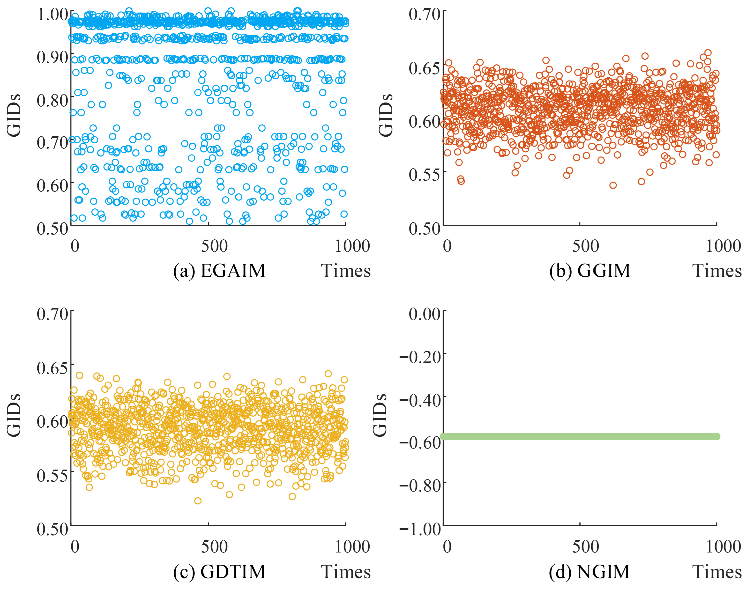
In the grey incidence analysis of panel data, if changes in the arrangement order of objects lead to changes in the correlation results, it indicates that the model needs improvement or is more suitable for analyses where the arrangement order of objects is fixed. In this subsection, we used Monte Carlo analysis to verify and analyze this characteristic of the model. In this study, there are 13 cities, resulting in 13! possible sorting methods. We selected 1000 non-repetitive permutations from them and calculated the correlation degree of the comparison model for each, with the results shown in Figure 8.

It can be seen from Figure 8 that the GIDs of EGAIM, GGIM, and GDTIM will all change with the change in the object arrangement order. This indicates that when analyzing cases where the arrangement order of objects is not fixed, it is necessary to carefully select the aforementioned comparison models (EGAIM, GGIM, and GDTIM). From the results of the Monte Carlo simulation, NGIM is suitable for cases where the arrangement order of objects is not fixed. Because, regardless of how the arrangement order of the objects changes, it will not affect the calculation results of the GIDs of NGIM. This is fully consistent with Property 2 of our model.

3.3.3. Analysis of Model Stability

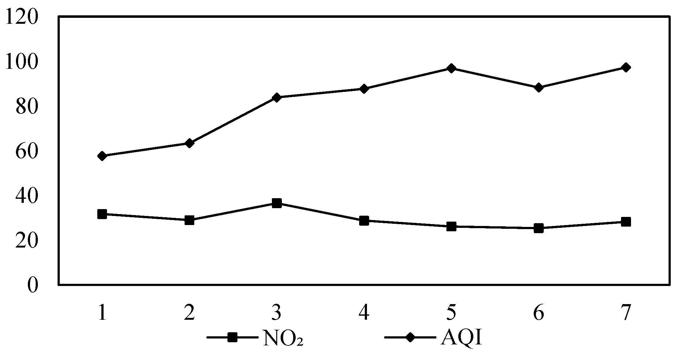
In the three comparison models, both GGIM and GDTIM can reflect the positive and negative of the coefficients. The grey incidence model can reflect positive or negative associations, so the method for calculating grey incidence degree is important. To verify this, we use actual examples below to demonstrate it. We choose the monthly data of AQI and NO₂’s monthly AQI from January to July 2016, which have been shown in Figure 9, and deeply analyze the reasons why the grey incidence model can reflect the positive and negative association that may have low stable robustness.

For the selected data, the coefficients and degrees calculated by the three models are shown in

Table 8. The coefficients and degrees of the three models.

	Time	GGIM	GDTIM	NGIM
GIC	1	−0.9560	−0.7702	−0.6974
	2	0.8667	0.6963	−0.6209
	3	−0.9447	−0.6838	−0.5197
	4	−0.9116	−0.6842	−0.4418
	5	0.8914	0.7868	−0.3754
	6	0.9151	0.8322	−0.4188
	7	-	-	−0.3841
GID		−0.0232	0.0295	−0.4940

. Within Table 8, the leftmost data indicates the coefficients or degree of the models; the second column, whose header is “time”, is the time point of the research data. The main part of the table shows the coefficients and degrees of the three models. It is worth noting that GGIM and GDTIM calculate the coefficients based on adjacent data, so seven data will generate six coefficients, resulting in an empty position corresponding to Time 7.

From the calculation results of the degrees in Table 8, the GID of NGIM is −0.4940. The scope of its GIC is [−0.6974, −0.3841]. Therefore, the degree of actual correlation between GIC and GID is similar. On the contrary, the degrees of GGIM and GDTIM are near 0, and the absolute values of the degrees are small. Meanwhile, all the absolute values of the coefficients of them are greater than 0.6838, which indicates that the two models consider a strong correlation between NO₂ and AQI when calculating the coefficients. The results of the grey incidence degree and grey incidence coefficient are contradictory. The root of this question is to directly take the average of the coefficients in the degree, which has been simply proved by Sun et al. [28]. The following content will be verified through Monte Carlo analysis.

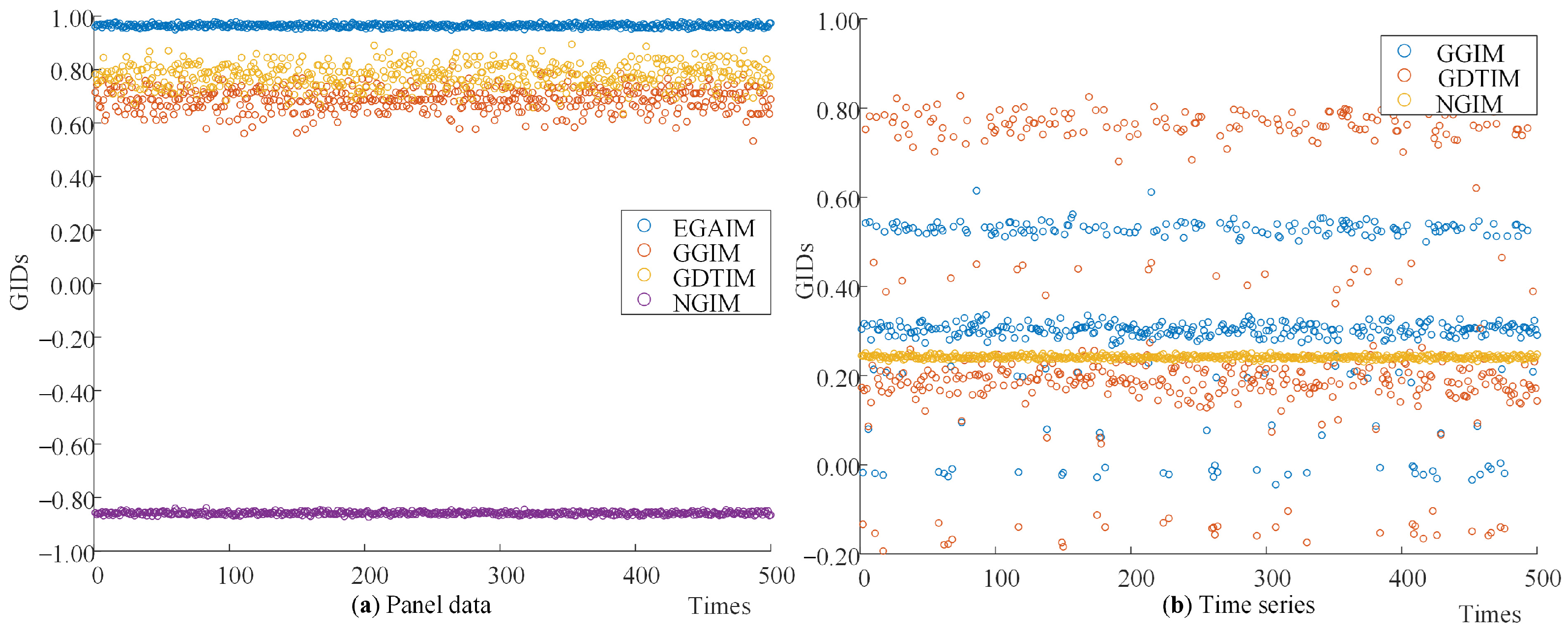
To enhance the credibility of the above analysis results, we conducted two sets of Monte Carlo analyses. One set was related to panel data, using the panel data of six pollutants in BJ and TJ from March 2017 to September 2017 for analysis; the other set was related to time series, using the CO and monthly AQI data from March 2017 to September 2017 for analysis. The experimental data range of these two sets of Monte Carlo analyses was set as the interval data fluctuating 5% up and down based on the above experimental data, and the experimental data sequence was composed of randomly selected data within the interval. In 500 repeated experiments, the selected models were calculated respectively according to the randomly selected sequences, with the results shown in Figure 10. It should be noted that EGAIM is not suitable for time series, so the results of EGAIM do not appear in Figure 10.

It can be seen from Figure 10a that when the experimental data is panel data, the GIDs of EGAIM and NGIM do not change significantly due to data fluctuations. In contrast, GGIM and GDTIM show more significant changes compared with EGAIM and NGIM. Moreover, as can be seen from Figure 10b, when the experimental data is time series, the GIDs of NGIM do not change significantly due to data fluctuations, but the results of GGIM and GDTIM obviously show the phenomenon of multiple data clustering intervals. This fully indicates that GGIM and GDTIM have low stability.

3.3.4. Analysis of the Influence of Sequence Volatility on NGIDs

This section will deeply analyze the influence of the anti-fluctuation factors on grey incidence degree, and compare the new model with the classic nearness grey incidence model proposed by Liu et al. [38]. Since the time scale of panel data involved in this paper is larger than the number of objects, it is easier to analyze the effect of relative volatility in the time dimension. Therefore, the impact of relative volatility will be analyzed in the time dimension.

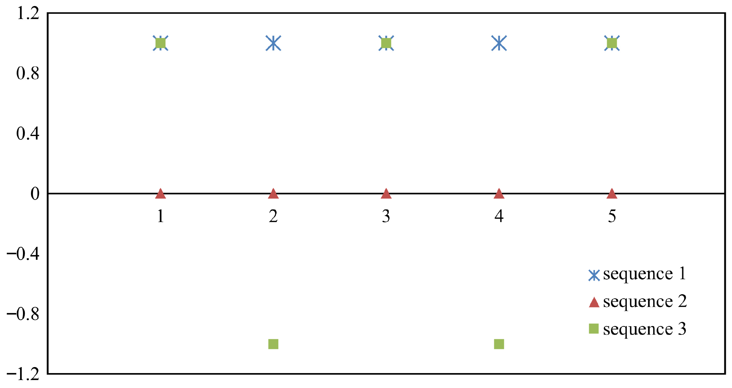
As for why relative volatility is considered in the nearness grey incidence model, it will be introduced in the following example. The example data is drawn in Figure 11 in the form of a scatter plot. The horizontal data represent the time points, while the vertical data represent the numerical values. The data of sequence 1 and sequence 2 are 1 and 0, respectively. The data of sequence 3 is alternating 1 and −1. Sequence 2 is used as the benchmark sequence. The calculation results of the classical nearness grey incidence model and the proposed model in this paper are listed in

Table 9. Grey incidence degrees for sample data.

Indicators	CNGIM	NGIM
Sequence 1-Sequence 2	0.2222	0.5073
Sequence 3-Sequence 2	0.6667	0.2934

. Within Table 9, the first column represents the sequence combination for calculating the nearness degree. CNGIM and NGIM are the abbreviations for the classical nearness grey incidence model and the proposed model.

The calculation results of the two models in Table 9 are diametrically opposite. The calculation results of CNGIM show that sequence 3 is closer to sequence 2, while the model in this paper considers that sequence 1 is closer to sequence 2. Actually, from each value of these sequences, the absolute distance between sequence 3 and sequence 2 and the absolute distance between sequence 1 and sequence 2 is always 1. That is to say, from the perspective of absolute distance, the nearness degree between two sequence combinations should be the same. But sequence 3 sometimes calculates the coefficients with sequence 2 from a direction greater than sequence 2, and sometimes calculates its coefficients with sequence 2 from a direction less than sequence 2. We believe that this uncertainty will reduce the absolute value of the nearness degree to a certain extent. Therefore, the new model can well distinguish the nearness grey incidence degree between sequences with the same absolute distance but different fluctuation conditions.

4. Conclusions

Since many problems in social life should consider the direction of nearness when judging whether the two are close, this paper constructs a new nearness grey incidence model suitable for panel data. Different from the traditional grey incidence model, the proposed model is not limited by the amount of calculation data, and the amount of data does not affect the calculation effect of the model.

From the perspective of model construction, the new model mainly has the following characteristics. First, it can reflect both the degree of nearness and the direction of nearness. The sign of the nearness grey incidence degree indicates the approach direction, and the absolute value of the nearness grey incidence degree indicates the degree of nearness. Second, when the order of objects is changed, the calculation results of the model will not change due to the change in the order of objects. Third, the relative volatility between sequences is incorporated into the model construction, which can better distinguish the sequences with the same absolute degree of nearness but different relative fluctuations. Fourth, the new model has updated the calculation method of the degree obtained by the coefficients, and the stable robustness is stronger.

In the case study part, this paper measures the major pollutants and analyzes the spatiotemporal distribution of six major pollutants in BTH from 2016 to 2024. It was found that PM_2.5, PM₁₀ and O₃ were the major pollutants during 2016–2024. In addition, the six pollutants all have seasonal distribution characteristics, among which the seasonal distribution characteristics of PM_2.5 and O₃ are significant, and the seasonal distribution characteristics of PM₁₀ and NO₂ are weaker than the former two; thirdly, based on the data from 2024, the NGIDs between 2016–2023 and 2024 conclude that the overall pollution in BTH has gradually improved; fourthly, taking Beijing as the benchmark, we calculated the degree between other cities of BTH and Beijing, and then the severity of different pollutants in BTH and in Beijing was compared; finally, we compared data with the traditional grey incidence model suitable for panel data; the proposed model was verified to have two important properties, no ordinal effect and strong stable robustness. Subsequently, the importance of adding the anti-fluctuation factor into the model was proved.

Up to this point, the proposed nearness grey incidence model has prominent advantages in analyzing practical problems and contrast with the other competing models, but there remains room for improvement. For future work, the applications of the model in the field of data stream analysis and spatiotemporal data analysis will be expanded. Additionally, the influence of meteorological factors on air pollution is also one of the key research directions for the future.