Machine Learning Calibration Transfer for Low-Cost Air Quality Sensors: Distance-Based Uncertainty Quantification in a Hybrid Urban Monitoring Network

Abstract

Low-cost air quality sensors enable dense urban monitoring networks but require calibration against reference-grade instruments. While machine learning calibration is well-established for co-located sensor pairs, applying these calibrations to sensors deployed far from any reference station—the operational reality for most network sensors—lacks systematic methodology. We address this gap using 24 months of hourly data (August 2023–July 2025) from Sofia, Bulgaria, where five official reference stations (Executive Environmental Agency) operate alongside 22 AirThings low-cost sensors, four of which are co-located. Random Forest models achieved $R^2\in (0.53,0.75)$ across PM_2.5, PM₁₀, NO₂, and O₃, representing from 40% (for O₃) to 408% (for PM_2.5) improvement over Multiple Linear Regression baselines. Using leave-one-station-out spatial cross-validation, we derived pollutant-specific uncertainty growth rates ($\alpha$) from 3.84% to 5.62% per km, characterizing how calibration uncertainty increases with distance from reference stations (statistically significant for PM₁₀ and O₃, $p<0.05$). Applied to 18 non-co-located sensors, the framework generated 1.2 million calibrated hourly measurements with 95% prediction intervals over the study period. Co-location sites spaced 6 km apart achieve a less than 30% uncertainty increase at network midpoints, within EU Air Quality Directive thresholds for indicative monitoring. These empirically derived $\alpha$ parameters enable network planners to predict measurement reliability at arbitrary sensor locations without ground-truth validation, providing evidence-based guidance for cost-effective hybrid monitoring network design.

1. Introduction

Urban air quality monitoring has become a pressing public health priority as cities worldwide grapple with the impacts of pollution on respiratory health, cardiovascular disease, and overall environmental quality [1,2,3]. Traditional monitoring approaches rely on official reference stations that provide highly accurate measurements but face a fundamental constraint: their high cost limits spatial coverage, leaving vast urban areas unmonitored. This sparse coverage makes it difficult to capture the fine-scale spatial variability of air pollution that exists within cities, where concentrations can vary significantly across neighborhoods due to local traffic patterns, industrial sources, and geographic features. Recent advances in sensor technology have introduced low-cost air quality sensors as a potential solution [4], offering the promise of dense monitoring networks at a fraction of the cost of traditional stations [5,6]. However, these sensors present their own challenges, particularly around calibration accuracy and data quality assurance. We analyze 24 months of hourly data (August 2023–July 2025), deliberately spanning two complete winter heating seasons to capture inter-annual variability and the full range of pollution conditions typical in Central European cities. This extended temporal coverage, combined with exceptional sensor data completeness (96.9% average data availability), provides a robust foundation for developing and validating calibration transfer methodologies.

The core challenge lies in integrating two fundamentally different monitoring systems: official reference stations that deliver traceable, quality-assured measurements but with limited spatial coverage, and low-cost sensor networks that enable dense monitoring but suffer from calibration uncertainties and sensor drift. While official stations operated by environmental agencies provide the gold standard for air quality data and are used for regulatory compliance, their expansion is financially prohibitive for most municipalities. Low-cost sensors, on the other hand, can be deployed in large numbers to reveal spatial pollution patterns, but their raw measurements often deviate significantly from reference-grade instruments due to cross-sensitivities, temperature dependencies, and gradual calibration drift. This creates a dilemma for cities seeking to expand their monitoring capabilities: invest heavily in a few additional reference stations, or deploy many low-cost sensors with uncertain data quality. This study addresses this challenge using data from Sofia, Bulgaria, where a unique opportunity exists to examine both systems operating in parallel–5 official reference stations operated by the Executive Environmental Agency (ExEA), located in the Pavlovo, Hipodruma, Nadezhda, Mladost, and Druzhba neighborhoods, alongside 22 AirThings low-cost sensors deployed throughout the city, with 4 sensors co-located within meters of official stations. A unique characteristic of this dataset is that while all reference stations measure PM₁₀, NO₂, and O₃, only one station (Hipodruma) provides PM_2.5 measurements. This creates an opportunity to examine calibration transfer under varying data availability constraints, with PM_2.5 calibration relying on a single co-located pair while other pollutants benefit from four independent training locations.

Three critical gaps prevent the effective integration of official and low-cost monitoring systems into validated hybrid networks. First, while co-located sensors can be calibrated against nearby reference stations, the vast majority of low-cost sensors are deployed in locations without proximate reference measurements, creating a calibration transfer problem that has not been systematically addressed in the literature. Second, operational frameworks that guide municipalities on how to strategically deploy and maintain hybrid networks are largely absent, leaving cities without clear implementation pathways. Third, quality assurance protocols for low-cost sensor data remain underdeveloped, particularly regarding uncertainty quantification and transparent communication of data reliability to policy makers and the public.

This study introduces a machine learning-based calibration transfer framework for creating validated hybrid air quality monitoring networks that combine the accuracy of official reference stations with the spatial density of low-cost sensor arrays. Our approach develops calibration models using co-located sensor pairs and then systematically transfers these calibrations to non-co-located sensors through transfer learning techniques that account for spatial distance, meteorological conditions, and measurement uncertainty. We implement and compare two machine learning calibration methods–Multiple Linear Regression as a baseline and Random Forest as an ensemble approach–achieving $R^2\in (0.53,0.75)$ across pollutants for operational calibration transfer. A key innovation is our distance-based uncertainty quantification framework that predicts calibration uncertainty as a function of spatial separation from reference stations (uncertainty growth rates: 3.8–5.6% per km; statistically significant for PM₁₀ and O₃, with consistent trends for PM_2.5 and NO₂), enabling practitioners to estimate measurement reliability for sensors deployed without ground-truth validation. This framework addresses a longstanding question in the sensor community: How sparse can co-location infrastructure be while maintaining acceptable calibration quality? Our analysis demonstrates that co-location sites spaced 6 km apart achieve <30% uncertainty increase at network midpoints, enabling cost-effective city-wide monitoring while maintaining transparent quality assurance.

The remainder of this paper is organized as follows. Section 2 reviews the relevant literature on low-cost air quality sensors, machine learning calibration methods, transfer learning applications, hybrid monitoring networks, and quality assurance frameworks. Section 3 describes our methodology, including the Sofia case study setup, data preprocessing, calibration model development, transfer learning implementation, and quality flagging system design. Section 4 presents results from calibration model evaluation, transfer learning performance, and network optimization analysis. Section 5 discusses the implications for urban air quality monitoring policy and practice, addresses limitations, and proposes future research directions. Section 6 concludes with practical recommendations for cities seeking to implement hybrid monitoring networks.

2. Literature Review

2.1. Low-Cost Air Quality Sensors

The past decade has witnessed rapid development in low-cost air quality sensing technology, driven by advances in miniaturized sensors, wireless communication, and affordable computing platforms [5]. These sensors, typically costing between $100 and $1000, measure particulate matter (PM_2.5, PM₁₀), gaseous pollutants (NO₂, O₃, CO), and meteorological variables using optical, electrochemical, or metal-oxide semiconductor technologies. Field deployments have demonstrated that low-cost sensors can capture meaningful spatial and temporal pollution patterns, revealing hotspots and gradients that official monitoring networks miss entirely due to their sparse coverage [6]. However, these sensors face well-documented limitations that complicate their use in scientific and regulatory applications. Cross-sensitivities to humidity, temperature, and interfering gases can introduce significant measurement errors. Sensor drift over time degrades calibration accuracy, with performance typically declining within months of deployment. Inter-sensor variability means that even sensors from the same manufacturer and model batch can produce different readings under identical conditions.

Validation studies comparing low-cost sensors against reference instruments have yielded mixed results, with correlation coefficients ranging from strong agreement $(R^2>0.8)$ under controlled conditions to poor performance $(R^2<0.5)$ in challenging field environments. The literature reveals that raw sensor measurements often require substantial calibration corrections before they can be considered reliable. Various calibration approaches have been proposed, from simple linear corrections to more sophisticated methods accounting for environmental cofactors [7], but most studies focus exclusively on co-located calibration scenarios where sensors sit directly next to reference stations. This leaves a critical gap: how to calibrate the majority of sensors deployed in locations far from any reference station.

2.2. Machine Learning Calibration Methods

Machine learning has emerged as a powerful tool for improving low-cost sensor accuracy by learning complex, nonlinear relationships between sensor readings, environmental conditions, and true pollutant concentrations [8]. Multiple Linear Regression (MLR) serves as the baseline approach in many studies, using sensor outputs and meteorological variables as predictors of reference measurements [9]. While interpretable and computationally efficient, MLR struggles to capture nonlinear sensor responses and complex interactions between variables. Random Forest models have shown superior performance in numerous calibration studies [10], effectively handling nonlinearities, variable interactions, and outliers without requiring extensive feature engineering. These ensemble methods consistently outperform linear models, achieving correlation improvements of 0.1–0.3 in $R^2$ values [11].

Neural networks and deep learning approaches represent the cutting edge of sensor calibration research, with architectures ranging from simple feedforward networks to more complex convolutional and recurrent designs [12]. These models can automatically extract relevant features from high-dimensional input data and learn hierarchical representations of sensor behavior [13]. Long Short-Term Memory (LSTM) networks have recently been applied to sensor calibration with the specific goal of modeling temporal dependencies and capturing sensor drift dynamics. LSTMs can learn how sensor accuracy degrades over time and potentially provide adaptive calibration that adjusts as sensors age. However, these advanced methods require substantial training data and computational resources, and their “black box” nature complicates interpretation and diagnostic analysis when calibrations fail.

Systematic algorithm comparisons confirm this hierarchy: gradient tree boosting, AdaBoost, and neural networks all outperform linear baselines in controlled benchmarks, but no single method consistently dominates across sensor types and environments [14]. Recent studies specifically targeting calibration propagation (applying a model trained at one node to geographically separated nodes) report that RF and gradient boosting maintain acceptable accuracy when source and target sites share similar microenvironments, while LSTM networks offer additional gains for pollutants with strong temporal structure [15,16].

Prior work has specifically evaluated supervised and unsupervised machine learning approaches for calibrating low-cost air quality sensors in urban deployments, consistently finding ensemble methods superior to linear baselines [17]. Despite this methodological diversity, a critical limitation persists across the literature: nearly all machine learning calibration studies train and validate models exclusively on co-located sensor-reference pairs. The question of how well these models transfer to sensors deployed elsewhere—spatially separated from training locations–remains largely unexplored. This represents a fundamental gap because the practical value of low-cost sensor networks depends precisely on deploying sensors where reference stations do not exist.

The study in [18] proposes machine learning calibration methods which use a high-cost instrument as a reference to improve the accuracy of networks of low-cost sensors. The authors combine three models for machine learning: linear regression, random forest, and Gradient Boosting Regression. In [19], the integration of machine learning and neural networks for the calibration of a low-cost nitrogen dioxide sensor is proposed. Tastan [20] developed the Internet of Things (IoT)-based air quality monitoring system. The system is tested by applying several machine learning algorithms as follows: Decision Tree (DT), Linear Regression (LR), Random Forest (RF), k-Nearest Neighbors (kNN), AdaBoost (AB), Gradient Boosting (GB), Support Vector Machines (SVM), and Stochastic Gradient Descent (SGD). In [21], the authors apply Linear Regression (LR), Random Forest (RF), Gradient Boosting (GB), k-nearest Neighbors (KNN), and Neural Networks (NN) for calibration of low-cost sensors for monitoring PM_2.5. They apply k-fold cross-validation methods to ensure the robustness of the performance of the model.

2.3. Transfer Learning in Sensor Networks

Transfer learning, the process of applying knowledge gained from one task or domain to a different but related task or domain [22,23], has seen limited application in air quality sensor calibration despite its potential relevance. The broader environmental monitoring literature includes examples of spatial transfer, where models trained at one location are applied to another, and temporal transfer, where models trained during one time period are applied to later periods. These studies demonstrate that transfer learning can work reasonably well when source and target domains share similar characteristics, but often requires domain adaptation techniques to account for systematic differences.

In the air quality sensor context, a few recent studies have begun exploring calibration transfer [8,24], typically by training models on co-located sensors and applying them to nearby non-co-located sensors, sometimes with correction factors based on meteorological similarity or spatial proximity. However, these efforts remain exploratory and lack systematic frameworks for quantifying transfer uncertainty, determining when transfer is appropriate, and adapting transferred calibrations to local conditions. No comprehensive methodology exists for implementing calibration transfer across an entire sensor network with varying distances from reference stations, diverse microclimatic conditions, and heterogeneous sensor characteristics. This gap is particularly problematic for operational deployments where most sensors will necessarily be far from reference stations.

2.4. Hybrid Monitoring Networks

The concept of hybrid monitoring networks—integrating official reference stations with low-cost sensor arrays—has gained traction as a pragmatic approach to expanding spatial coverage while maintaining data quality [25,26]. Several pilot deployments in cities worldwide have demonstrated the feasibility of operating both systems in parallel, with reference stations providing calibration anchors and validation data while low-cost sensors fill in spatial gaps. Co-location studies, where low-cost sensors are deliberately placed alongside reference instruments, have become standard practice for developing calibration equations and assessing sensor performance under real-world conditions [27].

However, the literature on hybrid networks reveals a significant gap in operational guidance. While researchers have successfully demonstrated hybrid network concepts in controlled deployments, cities lack clear frameworks for making strategic decisions about network design: how many reference stations are needed as calibration anchors, where to place them for maximum network benefit, how to optimize low-cost sensor placement to maximize coverage while ensuring calibratability, and how frequently sensors require recalibration. Cost-benefit analyses comparing hybrid network expansion strategies against traditional reference-station-only expansion are largely absent from the literature, making it difficult for municipalities to justify investments in hybrid approaches to policymakers and funding agencies.

2.5. Quality Assurance and Uncertainty Quantification

Quality assurance (QA) for low-cost sensor data presents unique challenges distinct from traditional reference monitoring [28]. While reference stations operate under strict QA/QC protocols with regular calibration checks, zero/span tests, and performance audits, comparable protocols for low-cost sensor networks remain underdeveloped. The literature includes various proposals for automated QA procedures: statistical outlier detection, temporal consistency checks, spatial coherence analysis, and comparison against co-located reference data when available [29]. However, these methods typically flag potentially problematic data without providing quantitative uncertainty estimates that would allow users to assess fitness for specific purposes.

Uncertainty quantification–providing confidence intervals or prediction intervals for calibrated measurements–is essential for regulatory and policy applications but is rarely implemented in low-cost sensor deployments [30]. Some studies have explored uncertainty estimation using machine learning prediction intervals, ensemble model variance, or residual analysis from co-located comparisons [31]. A particularly important gap is the need for distance-based uncertainty models that recognize a fundamental reality: measurements from sensors located far from reference stations inherently carry greater calibration uncertainty than those close to reference stations. Such models would enable transparent communication of data reliability, allowing end users to make informed decisions about whether data quality is sufficient for their intended application, whether for community awareness, scientific research, or regulatory compliance.

Furthermore, existing quality flagging systems, when they exist at all, tend to be binary (pass/fail) rather than providing graduated quality levels that reflect the reality that data can have varying degrees of reliability suitable for different purposes. Transparent, automated quality flagging systems that clearly communicate confidence levels based on objective criteria—distance to reference stations, calibration model performance, measurement uncertainty—would significantly enhance the credibility and usability of hybrid network data.

2.6. Research Gaps and Study Objectives

Prior studies have established important foundations for calibration transferability research. Van Zoest et al. [32] evaluated spatial transferability of three calibration methods for NO₂ electrochemical sensors across a 35-node network in Eindhoven, finding that calibration parameters do not generalise well across locations. Wei et al. [33] demonstrated the importance of temperature-sensitive corrections for long-term NO₂ network calibration. De Vito et al. [34] documented “concept drift” when electrochemical NO₂ sensor nodes are relocated to different microenvironments, concluding that static field calibrations degrade with relocation. These three studies collectively establish that calibration transfer for gas-phase sensors is problematic; they address NO₂ measured by electrochemical sensors exclusively.

Three interconnected gaps remain. First, calibration transfer for optical particulate matter sensors (PM_2.5, PM₁₀) has received far less systematic attention; the different physical measurement principles and interference mechanisms require independent investigation. Second, none of the prior works quantify how much uncertainty grows as a function of spatial separation from reference infrastructure, leaving network planners without actionable co-location spacing guidance. Third, the simultaneous treatment of calibration relocation and cross-node sensor-to-sensor fabrication variance has not been addressed within a unified uncertainty framework.

This study addresses these gaps using data from Sofia, Bulgaria’s hybrid monitoring network. We develop and evaluate RF and MLR calibration models on co-located sensor pairs across four pollutants (PM_2.5, PM₁₀, NO₂, O₃), then introduce a distance-based uncertainty quantification framework that translates spatial separation into calibration uncertainty bounds. We provide practical network design guidance demonstrating that co-location sites spaced 6 km apart achieve less than 30% uncertainty increase at network midpoints, within EU indicative monitoring thresholds.

3. Methodology

3.1. Study Area and Monitoring Network

Sofia, Bulgaria’s capital city with approximately 1.3 million residents, is situated in a geological basin surrounded by mountains, creating conditions favorable for temperature inversions that trap air pollutants, particularly during winter heating seasons, when particulate matter concentrations often exceed EU air quality standards. This topographic configuration makes Sofia an ideal case study for hybrid monitoring network development, as the city experiences significant spatiotemporal variability in pollution levels that sparse reference station networks cannot adequately capture. Recent digital twin modeling of mobile-source emissions across Sofia’s urban area has further characterized this heterogeneous pollution landscape [35], underscoring the need for dense monitoring networks capable of resolving intra-urban concentration gradients.

3.1.1. Reference Monitoring Stations

The Executive Environmental Agency (ExEA) operates five official reference stations across Sofia, located in the Pavlovo, Hipodruma, Nadezhda, Mladost, and Druzhba neighborhoods. These stations employ reference-grade instrumentation following European Standard methods [36]: gravimetric measurement (EN 12341:2023) for particulate matter with beta-attenuation monitors for continuous PM₁₀ monitoring [37], chemiluminescence (EN 14211:2024) for nitrogen dioxide and nitrogen monoxide [38], and ultraviolet photometry (EN 14625:2024) for ozone [39]. A critical limitation of this network is that only the Hipodruma station measures PM_2.5, creating substantial data scarcity for fine particulate matter analysis across the city, a significant constraint given that PM_2.5 is the pollutant most strongly associated with adverse health outcomes. All reference stations measure PM₁₀, NO₂, O₃, and CO, along with meteorological variables including temperature, atmospheric pressure, relative humidity, wind speed, and wind direction.

3.1.2. Low-Cost Sensor Network

The Sofia Municipality deployed 22 AirThings low-cost air quality sensors throughout the city as part of an initiative to expand spatial monitoring coverage. These sensors employ optical particle counters for particulate matter measurement and electrochemical cells for gaseous pollutants, measuring PM_2.5, PM₁₀, NO₂, O₃, and CO at hourly resolution. While substantially less expensive than reference instrumentation (approximately $200–500 per sensor versus $20,000–50,000 per reference station), these devices face well-documented accuracy challenges including temperature and humidity cross-sensitivities, calibration drift, and inter-sensor variability [5,6]. Critically, four sensors (AT1, AT3, AT11, AT15) were deliberately co-located within meters of reference stations (Hipodruma, Druzhba, Mladost, and Pavlovo, respectively), creating a unique natural experiment for developing and validating calibration transfer methodologies. The fifth reference station (Nadezhda) lacked a co-located sensor and was therefore excluded from calibration training and spatial cross-validation.

The monitoring stations are Develiot Urban Air Quality Monitoring Stations (UAQMS, v7.3, March 2022 hardware generation; Develiot, Sofia). Gaseous pollutants are measured by electrochemical cells: NO₂, O₃, and CO operate in the low-concentration urban range (0–1 ppm for NO₂/O₃; 0–10 ppm for CO) with a resolution of <10 ppb and a manufacturer-specified operational lifespan of 12 months, after which sensor replacement is required to maintain calibration stability. Particulate matter is measured by a laser-scattering optical particle counter (range 0–1000 μg/m³, resolution 0.1 μg/m³, 12-month operational lifespan). The integrated meteorological sensor provides temperature (accuracy ±0.2 °C), relative humidity (±1.5%), and atmospheric pressure (±0.5 hPa). All sensing elements are housed in an IP65-rated enclosure with active climatization, a patented thermal management system that reduces temperature and humidity cross-sensitivities inherent to electrochemical and optical sensing technologies.

3.2. Data Collection and Temporal Coverage

We analyze 24 months of hourly air quality and meteorological data spanning 1 August 2023 through 31 July 2025, yielding 17,521 hourly timestamps. This extended temporal coverage was deliberately selected to capture two complete winter heating seasons (November–March), when Sofia experiences the most severe air quality episodes due to residential heating combined with meteorological conditions that trap pollutants. Prior calibration studies have demonstrated that training data spanning at least one complete annual cycle is essential for capturing seasonal variations in sensor response [11], and multi-year datasets reduce the risk of overfitting to atypical meteorological conditions [40]. The dataset encompasses the full range of seasonal variability typical in Central European continental climates, from winter temperature inversions with stagnant air masses to summer photochemical ozone formation events.

Data completeness exceeded expectations for both monitoring systems. Reference stations achieved 95–99% data availability across pollutants (PM₁₀: 97.2%, NO₂: 98.6%, O₃: 98.4%), with the exception of PM_2.5 at Hipodruma (93.7% complete). These availability rates exceed the 90% data capture requirement specified in the EU Air Quality Directive for fixed measurements [36]. The low-cost sensor network demonstrated exceptional reliability with 96.9% average data availability across all 22 sensors, ranging from 89.9% (AT5) to 99.6% (AT17, AT20), substantially higher than the 50–80% availability commonly reported in low-cost sensor deployments [31].

3.3. Data Preprocessing and Quality Control

All raw data underwent systematic quality control procedures following EPA guidance for low-cost sensor evaluation [41] and implemented in Python using pandas (version 2.0+) and numpy (version 1.24+). Timestamps were standardized to UTC and synchronized to hourly resolution across both monitoring systems, ensuring temporal alignment between sensor and reference measurements–a critical step given that even small timing offsets can introduce spurious calibration errors [7].

Physical range validation flagged measurements outside plausible bounds based on historical extremes observed in Sofia and surrounding regions: PM_2.5 and PM₁₀ (0–1000 μg/m³), NO₂ andO₃ (0–500 ppb), temperature (−20 to 45 °C), relative humidity (0–100%), and atmospheric pressure (900–1050 hPa). The Rate-of-change filters identified implausible spikes (>200 μg/m³/h for PM, >100 ppb/h for gases), which typically indicate sensor malfunctions rather than genuine pollution events [29]. Missing data gaps shorter than three consecutive hours were forward-filled using the last valid observation, a conservative approach that avoids introducing interpolation artifacts while maintaining temporal continuity for time-series features. Longer gaps were preserved as missing values and excluded from model training.

Temporal features were extracted to enable machine learning models to capture diurnal and seasonal pollution patterns that reflect emission source activity and atmospheric dynamics [42]. Three integer-valued temporal features were included: hour of day (0–23), month (1–12), and a binary weekend indicator. These raw integer representations were retained rather than cyclically encoded, as the Random Forest algorithm assigns thresholds through recursive partitioning and does not require the numerical continuity assumptions that motivate sine-cosine transformation in distance-based or linear models.

Co-located sensor pairs were identified using Haversine distance calculations between AirThings sensor and ExEA reference station coordinates. Sensors within 5 m were classified as co-located, consistent with EPA recommendations that co-location distances should not exceed the inlet height of reference instruments to minimize microenvironmental differences [43]. This analysis identified four co-located pairs: Hipodruma ↔ AT1, Pavlovo ↔ AT15, Mladost ↔ AT11, and Druzhba ↔ AT3, yielding 69,064 synchronized hourly measurements across all four pairs, with 16,162 valid PM_2.5 observation pairs from Hipodruma ↔ AT1 specifically.

3.4. Calibration Model Development

Calibration models were trained exclusively on the four co-located sensor pairs to learn the relationship between low-cost sensor readings and co-located reference measurements. This co-location-based calibration approach, sometimes termed field calibration, has become standard practice in low-cost sensor research because it captures real-world sensor behavior under ambient conditions rather than controlled laboratory settings [8,11]. The fundamental calibration task is to estimate a function f such that:

$$C_{\mathrm{ref}}=f(C_{\mathrm{sensor}},\mathbf{M},\mathbf{T})+ϵ$$

(1)

where $C_{\mathrm{ref}}$ is the reference pollutant concentration, $C_{\mathrm{sensor}}$ is the low-cost sensor reading, $\mathbf{M}$ represents meteorological covariates (temperature T, relative humidity RH, atmospheric pressure P), $\mathbf{T}$ represents temporal features (hour, month, day of week), and $ϵ$ is irreducible error arising from measurement noise and unmodeled factors. The inclusion of meteorological covariates is essential because low-cost sensors exhibit well-documented cross-sensitivities: optical particle counters are affected by hygroscopic particle growth at high humidity [44,45], while electrochemical gas sensors show temperature-dependent baseline drift and sensitivity changes [46,47].

3.4.1. Model Specifications

Model A: Multiple Linear Regression (MLR) serves as an interpretable baseline, assuming additive linear relationships between predictors and reference concentrations [9]:

$$C_{\mathrm{ref}}={\beta }_0+{\beta }_1{C}_{\mathrm{sensor}}+{\beta }_{2}T+{\beta }_3\mathrm{RH}+{\beta }_{4}P+\sum _k{\beta }_k{\mathbf{T}}_k+ϵ$$

(2)

where coefficients $\beta$ are estimated via ordinary least squares. MLR provides a performance floor against which more complex models can be compared, and its coefficients offer direct physical interpretation (e.g., ${\beta }_3$ quantifies the humidity correction per percentage point RH).

Model B: Random Forest (RF), implemented via scikit-learn (version 1.3+), constructs an ensemble of decision trees trained on bootstrap samples with random feature subsets [48]. This ensemble approach has emerged as the dominant method for low-cost sensor calibration due to its ability to capture nonlinear sensor responses, automatic handling of variable interactions, and robustness to outliers [10,11]:

$${\widehat{C}}_{\mathrm{ref}}={\displaystyle \frac{1}{N_{\mathrm{trees}}}}\sum _{i=1}^{N_{\mathrm{trees}}}{T}_i(C_{\mathrm{sensor}},\mathbf{M},\mathbf{T})$$

(3)

Hyperparameters were selected via 5-fold cross-validation on the training set: $N_{\mathrm{trees}}=200$ (beyond which out-of-bag error stabilized), maximum tree depth = 15 (balancing model complexity against overfitting), minimum samples per leaf = 5 (preventing trees from memorizing individual observations), and maximum features per split = $\sqrt{p}$ where p is the number of predictors (the default for regression tasks that promotes tree diversity) [49]. The feature set for each pollutant model included: raw sensor reading, temperature, relative humidity, pressure, and cyclically-encoded temporal features (hour_sin, hour_cos, month_sin, month_cos, weekend indicator). Feature importance was quantified using the mean decrease in Impurity (MDI), which measures how much each feature contributes to reducing prediction variance in all decision tree splits [48].

3.4.2. Training and Evaluation Protocol

Data from co-located pairs were pooled across all available stations for each pollutant (four stations for PM₁₀, NO₂, O₃; one station for PM_2.5) and split chronologically: the first 80% of timestamps (19.2 months) for training and the final 20% (4.8 months) for independent testing. This temporal split, rather than random sampling, is critical for realistic performance estimation because it simulates the operational scenario where models trained on historical data must predict future measurements [50]. Random splits would allow information leakage across the temporal boundary, artificially inflating performance estimates.

Three complementary cross-validation strategies assessed model generalization across different dimensions of extrapolation:

• Temporal cross-validation: A single temporal hold-out fold was used for validation: models were trained on the first 18 months (August 2023–January 2025) and evaluated on the held-out final 6 months (February–July 2025). This fold evaluates whether calibration relationships remain stable over time or degrade due to sensor drift, seasonal regime shifts, or changes in emission sources.
• Seasonal cross-validation: Leave-one-season-out design (winter: December–February; spring: March–May; summer: June–August; fall: September–November). This tests whether models trained predominantly on one pollution regime (e.g., winter heating episodes) generalize to different seasonal conditions.
• Spatial cross-validation: Leave-one-station-out design for pollutants with multiple co-location pairs (PM₁₀,NO₂, O₃). This is the most stringent test, evaluating whether calibration relationships learned at one location transfer to geographically distinct sites with potentially different microenvironments, source mixtures, and sensor-specific characteristics [51]. Note:O₃ spatial CV was limited to three stations because the Mladost reference station does not measure ozone.

The production calibration models applied to all 22 sensors are subsequently retrained on the full 24-month co-location dataset; the 18-month split is a validation instrument only and does not limit the training data available for deployment.

The performance of the model was evaluated using three complementary metrics: coefficient of determination $\left(R^2\right)$, root mean square error (RMSE), and mean absolute error (MAE). $R^2$ captures the proportion of variance explained and enables comparison across pollutants with different concentration ranges; RMSE emphasizes large errors and is sensitive to outliers; MAE provides a robust central tendency measure of prediction error magnitude.

3.5. Calibration Transfer and Uncertainty Quantification

The 18 non-co-located sensors represent the primary operational challenge: how to provide calibrated measurements for sensors deployed 1–6 km from the nearest reference station, where no ground-truth reference data exist for validation. This calibration transfer problem–applying models trained at co-located sites to spatially distant sensors–is conceptually related to spatial prediction problems in geostatistics, where prediction uncertainty typically increases with distance from observation locations [52].

3.5.1. Transfer Methodology

For each non-co-located sensor, calibrated concentrations were generated by applying the trained Random Forest model directly to the sensor’s raw measurements and concurrent meteorological data. The underlying assumption is that sensors of the same model (AirThings) exhibit similar response characteristics, such that calibration relationships learned from co-located sensors transfer to non-co-located sensors of identical hardware [13]. This assumption is strongest when sensors are from the same manufacturing batch and have similar deployment ages, and weakest when inter-sensor variability is high, or sensors have experienced differential aging or damage.

3.5.2. Distance-Based Uncertainty Model

We developed a distance-based uncertainty quantification framework to provide realistic confidence bounds for transferred calibrations. The conceptual basis is that calibration uncertainty should increase with spatial separation from reference stations due to: (1) spatial heterogeneity in pollution source mixtures and atmospheric conditions that the calibration model was not trained on, (2) potential inter-sensor variability not captured by models trained on different sensor units, and (3) microenvironmental differences between co-located sites (often in controlled settings near official stations) and typical deployment locations [42].

We model measurement uncertainty as a linear function of distance:

$${\sigma }_j\left(d\right)={\sigma }_{\mathrm{base}}·\left(1+\alpha ·d_j\right)$$

(4)

where ${\sigma }_j\left(d\right)$ is the estimated prediction uncertainty for sensor j, ${\sigma }_{\mathrm{base}}$ is the baseline calibration uncertainty estimated as the intercept of a linear regression of RMSE against distance from spatial cross-validation results (representing expected uncertainty at zero distance from reference stations), $d_j$ is the Haversine distance to the nearest reference station (km), and $\alpha$ is the uncertainty growth rate parameter (km⁻¹). The linear form was chosen for parsimony and interpretability; more complex functional forms (exponential, power-law) were explored but did not significantly improve fit given the limited distance range (1–6 km) in our network.

The parameter $\alpha$ was estimated empirically using the spatial cross-validation results. In leave-one-station-out cross-validation, each held-out station provides an estimate of prediction error at a known distance from the training stations. By regressing absolute prediction residuals against distance across all held-out evaluations, we obtained pollutant-specific $\alpha$ estimates. This approach assumes that performance degradation observed when transferring to held-out co-located stations is representative of degradation expected when transferring to non-co-located sensors at similar distances, a reasonable approximation given that co-located stations span diverse microenvironments across Sofia.

3.5.3. Prediction Intervals

The distance-scaled uncertainty estimates provide 95% prediction intervals for each calibrated measurement:

$${\mathrm{PI}}_{95}\left(j\right)={\widehat{C}}_{\mathrm{sensor},j}\pm 1.96·{\sigma }_j\left(d\right)$$

(5)

assuming approximately normal prediction errors, which was verified by examining residual distributions from co-located calibration. These intervals communicate measurement reliability to end users: sensors near reference stations have narrow intervals reflecting high confidence, while peripheral sensors have wider intervals appropriately reflecting greater calibration uncertainty. This transparent uncertainty quantification addresses a key criticism of low-cost sensor deployments, that measurements are often presented without acknowledgment of their substantial uncertainty [30].

4. Results

4.1. Co-Location Calibration Performance

Table 1. Calibration model performance on co-located sensor test set.

Pollutant	Model	ntest	R2	RMSE (μg/m3)	MAE (μg/m3)
PM2.5	MLR	2408	0.147	11.52	7.84
	Random Forest	2408	0.745	6.30	4.00
PM10	MLR	9726	0.142	19.20	12.94
	Random Forest	9726	0.668	11.95	7.43
NO2	MLR	9882	0.199	16.94	13.21
	Random Forest	9882	0.532	12.94	9.77
O3	MLR	7540	0.532	21.56	17.48
	Random Forest	7540	0.745	15.91	12.52

summarizes the calibration performance of both models across all four pollutants on the held-out test set. Random Forest consistently outperformed MLR across all pollutants, with $R^2$ improvements ranging from 40% (O₃) to 407% (PM_2.5). Better results are in bold.

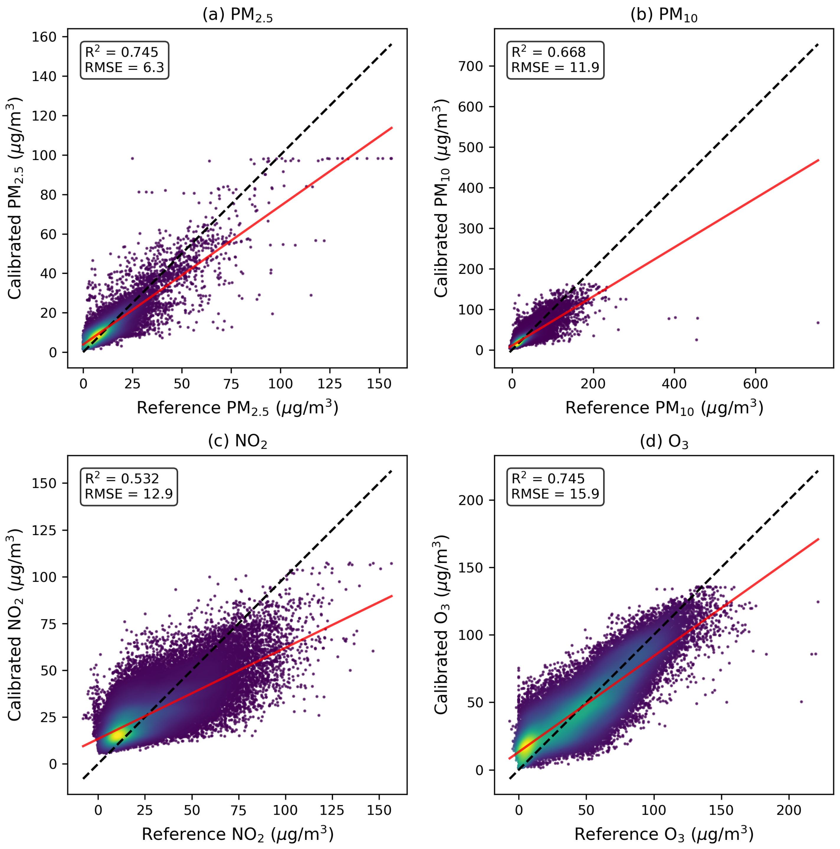
Figure 1 shows calibration scatter plots comparing Random Forest predictions against reference measurements for each pollutant.

Based on these results, Random Forest was selected as the operational calibration model for transfer to non-co-located sensors.

4.2. Cross-Validation Analysis

To assess model generalizability beyond the training period and locations, we conducted both temporal and spatial cross-validation experiments. The temporal cross-validation design trained models on the first 18 months of data and reserved the final 6 months as an independent test set, simulating the operational deployment scenario where calibration models must extrapolate to future time periods that may differ in pollution regimes and meteorological conditions. Under this temporal holdout design, MLR performance degraded substantially for some pollutants, with NO₂ dropping from $R^2=0.20$ to $R^2=-0.08$. Negative $R^2$ values indicate that predictions performed worse than simply using the training period mean as a constant predictor, suggesting that the linear model failed to capture temporal dynamics that differ between training and test periods. In contrast, O₃ maintained a more stable performance $(R^2=0.44)$, indicating that the drivers of ozone calibration are more temporally consistent. These results suggest that the importance of temporal factors varies substantially across pollutants.

Spatial cross-validation using a leave-one-station-out design provided critical insights about calibration transferability across Sofia’s monitoring network. In this experiment, Random Forest models were trained on three of the four co-located pairs and evaluated on the held-out fourth pair, rotating through all combinations.

Table 2. Random Forest spatial cross-validation results (leave-one-station-out). Results are shown for the full feature set, including temporal features (hour, month, weekend indicator) and for physical features only (temperature, pressure, humidity), to empirically assess the effect of temporal features on spatial calibration transfer.

Pollutant	Test Station	R2 (with Temporal)	R2 (Without Temporal)	RMSE (μg/m3)
PM10	Pavlovo	0.446	0.356	16.41
	Hipodruma	0.219	0.098	19.78
	Mladost	0.465	0.416	11.72
	Druzhba	0.174	0.127	18.87
NO2	Pavlovo	0.329	0.141	17.74
	Hipodruma	0.397	0.243	13.92
	Mladost	0.222	0.036	13.98
	Druzhba	−0.029	−0.282	18.72
O3	Pavlovo	0.437	0.385	24.87
	Hipodruma	−0.145	−0.311	28.92
	Druzhba	0.565	0.501	21.32

summarizes performance when each co-location site is held out for testing.

The variable performance across stations ($R^2$ ranging from $-0.15$ to $0.57$ with the full feature set) indicates that calibration transfer is not uniformly successful across all locations. Hipodruma shows particularly poor O₃ transfer performance, likely reflecting unique microenvironmental conditions at this central urban site, while Druzhba NO₂ also yields negative $R^2$, consistent with the pronounced NO₂ spatial gradient near this traffic-exposed location. Notably, temporal features (hour, month, weekend indicator) consistently improve spatial transfer performance across all three pollutants and all stations: mean $R^2$ increases from 0.25 to 0.33 for PM₁₀, from 0.03 to 0.23 for NO₂, and from 0.19 to 0.29 for O₃ when temporal features are included. This empirical result indicates that, for Sofia’s compact urban network, the shared diurnal and seasonal structure of emission sources across neighborhoods provides a generalizable signal rather than location-specific overfitting, as might be expected in a larger or more spatially heterogeneous city. This variability underscores the importance of the uncertainty quantification framework developed in Section 3.5.

Seasonal cross-validation (

Table 3. Seasonal cross-validation results (leave-one-season-out).

Pollutant	Test Season	ntrain	ntest	R2	RMSE (μg/m3)	MAE (μg/m3)
PM2.5	Winter	12,042	4005	0.223	17.13	9.74
	Spring	12,376	3671	0.345	5.43	3.93
	Summer	11,911	4136	−0.151	7.20	5.21
	Fall	11,812	4235	0.167	8.05	5.71
PM10	Winter	50,724	14,115	0.143	29.24	17.25
	Spring	47,580	17,259	0.223	13.58	9.35
	Summer	47,850	16,989	0.174	11.93	8.75
	Fall	48,363	16,476	−0.017	16.58	11.86
NO2	Winter	51,190	14,691	0.147	20.85	15.79
	Spring	48,596	17,285	−0.148	15.78	12.12
	Summer	48,711	17,170	0.096	11.86	8.88
	Fall	49,146	16,735	−0.013	20.25	14.73
O3	Winter	38,374	11,890	−0.026	21.65	17.36
	Spring	37,346	12,918	0.114	24.01	19.52
	Summer	37,310	12,954	0.461	22.35	17.34
	Fall	37,762	12,502	0.200	23.39	18.87

) revealed substantial variation in calibration performance across seasons. O₃ achieved the highest seasonal $R^2$ during summer $\left(0.46\right)$, reflecting the strong temperature-ozone relationship during photochemically active months. Conversely, PM_2.5 showed negative $R^2$ during summer $(-0.15)$, suggesting that calibration relationships developed during heating-season pollution episodes may not transfer well to summer conditions with different particle composition. NO₂ exhibited consistently modest performance across all seasons $(R^2\in (-0.15,0.15))$, indicating challenges in generalizing electrochemical sensor calibrations across seasonal emission and meteorological regimes.

To verify that RF extrapolation is not a concern in practice, we checked what fraction of transfer-site observations fall within the training feature space. Across all three pollutants, 99.5% of transfer observations ($n>300,000$) lie within the min–max bounds of the co-location training data for every feature; the only gap is 0.5% of temperature readings marginally outside the training range. RF extrapolation is therefore not a material source of error in this network.

4.3. Feature Importance Analysis

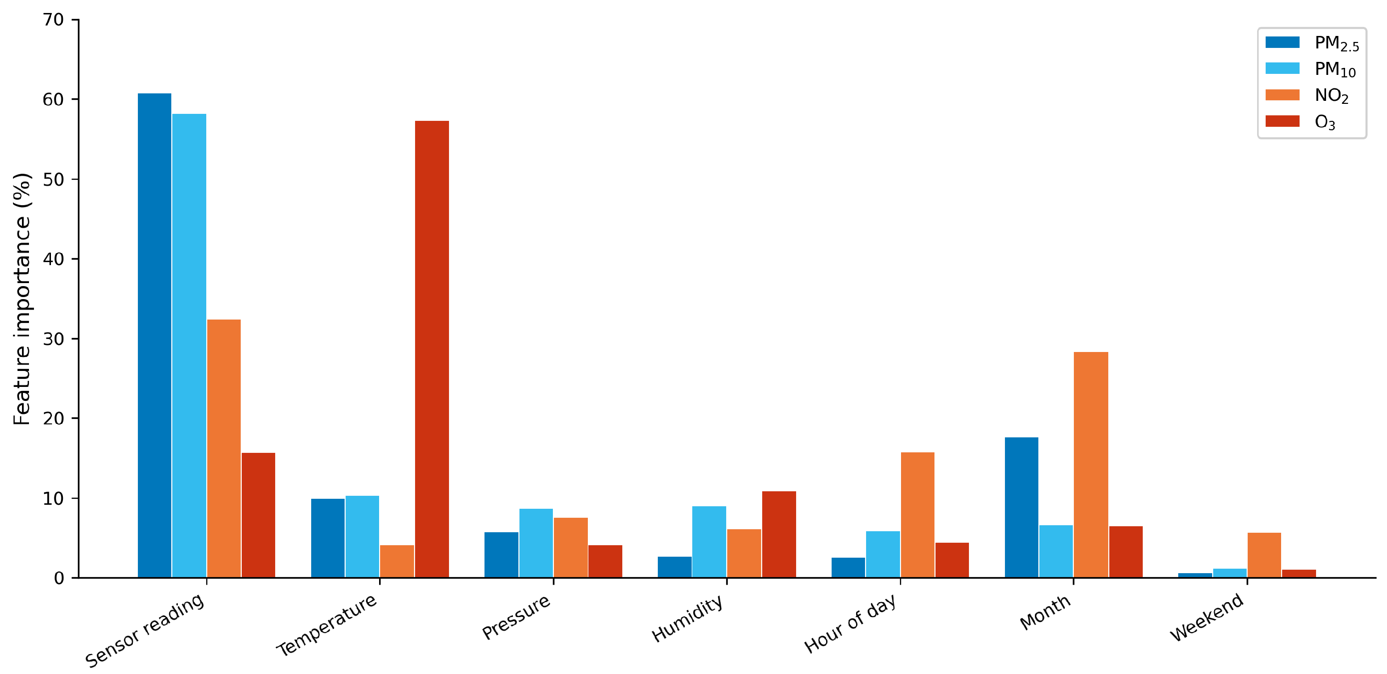
Random Forest feature importance analysis (Figure 2) reveals that fundamentally different calibration mechanisms operate across pollutant types. For particulate matter, the sensor readings themselves dominate the calibration model, contributing 60% of the total importance for PM_2.5 and 58% for PM₁₀. Temperature and seasonal features (encoded through month) add modest contributions of 10–18%, primarily capturing humidity-related optical interference in winter months. This pattern indicates that the optical particle counters in these low-cost sensors provide informative base signals that require only modest environmental correction to align with reference measurements.

The calibration mechanism for NO₂ differs markedly from that of particulate matter. Temporal features dominate the model, with month contributing 28% and hour of day contributing 16% of total importance, together exceeding the 32% contribution from the sensor reading itself. This pattern reflects the strong diurnal and seasonal cycles characteristic of NO₂ concentrations, driven by morning and evening traffic rush hours and seasonal variations in atmospheric mixing depth. The implication is that electrochemical NO₂ sensors require substantial temporal adjustment, and the calibration model essentially learns to predict typical NO₂ patterns for a given time of day and season, with the sensor reading providing secondary refinement.

Ozone calibration is dominated almost entirely by temperature, which accounts for 57% of feature importance while the sensor reading contributes only 16%. This finding reflects the well-documented temperature cross-sensitivity of electrochemical O₃ sensors, where the sensing element responds not only to ozone concentration but also strongly to ambient temperature. The calibration model thus primarily corrects for thermal artifacts rather than extracting an ozone-specific signal from the sensor output.

These non-linear sensor behaviours directly explain the large RF–MLR performance gap (average 246% improvement). Multiple Linear Regression can fit only a single slope per feature; it cannot represent the temperature-saturating response of EC O₃ sensors, the interaction between humidity and optical PM scattering, or the non-linear diurnal NO₂ profile. Random Forest partitions the feature space into local regions where each non-linearity is captured independently, which is precisely why ensemble methods outperform linear baselines so markedly for these sensor types.

These distinct calibration mechanisms have practical implications for sensor network design and transferability. Particulate matter sensors, where the sensor reading dominates calibration, may transfer more reliably across locations because the fundamental sensor response remains consistent. Gaseous sensors, in contrast, require careful attention to local temporal pollution patterns and temperature regimes, and calibrations developed at one location may not transfer as effectively to sites with different diurnal traffic patterns or thermal environments.

4.4. Calibration Transfer to Non-Co-Located Sensors

Having established Random Forest as the preferred calibration approach through the co-location experiments, we applied the trained models to calibrate measurements from the 18 non-co-located sensors distributed across Sofia. Over the 24-month study period, this transfer process generated a total of 1,207,809 calibrated hourly measurements, each accompanied by distance-scaled uncertainty estimates derived from the framework described in Section 3.5.

The calibrated measurements reveal the pollution landscape across Sofia’s urban area. Mean PM_2.5 concentrations of 14.5 μg/m³ indicate moderate fine particulate pollution that exceeds the WHO guideline of 5 μg/m³ but remains below the EU annual limit of 25 μg/m³. PM₁₀ levels are elevated at 27.3 μg/m³, reflecting contributions from road dust, construction activity, and residential heating during winter months. NO₂ concentrations average 28.9 μg/m³, consistent with traffic-dominated urban environments. Ozone levels are relatively high at 48.7 μg/m³, typical of continental European cities where strong solar radiation during summer drives photochemical production from precursor pollutants transported into the Sofia basin.

4.5. Spatial Uncertainty Quantification

A central question for network planners is how measurement uncertainty grows as sensors are deployed increasingly far from reference stations. To address this, we fitted linear uncertainty growth models relating prediction residual magnitude to distance from the nearest co-location site.

Table 4. Distance-based uncertainty growth parameters.

Pollutant	σbase (μg/m3)	α (km−1)	Growth (%/km)	R2	p-Value
PM10	20.26	0.0562	5.62	0.379	0.0066 **
PM2.5	9.30	0.0533	5.33	0.177	0.0819
NO2	17.47	0.0424	4.24	0.134	0.1350
O3	24.02	0.0384	3.84	0.260	0.0307 *

* p < 0.05, ** p < 0.01; Distance range: 1.0–5.6 km ($n=18$ sensors)

presents the fitted uncertainty growth parameters for all pollutants, including the baseline uncertainty at co-located sites (${\sigma }_{\mathrm{base}}$), the growth rate per kilometer ($\alpha$), and statistical significance of the distance effect.

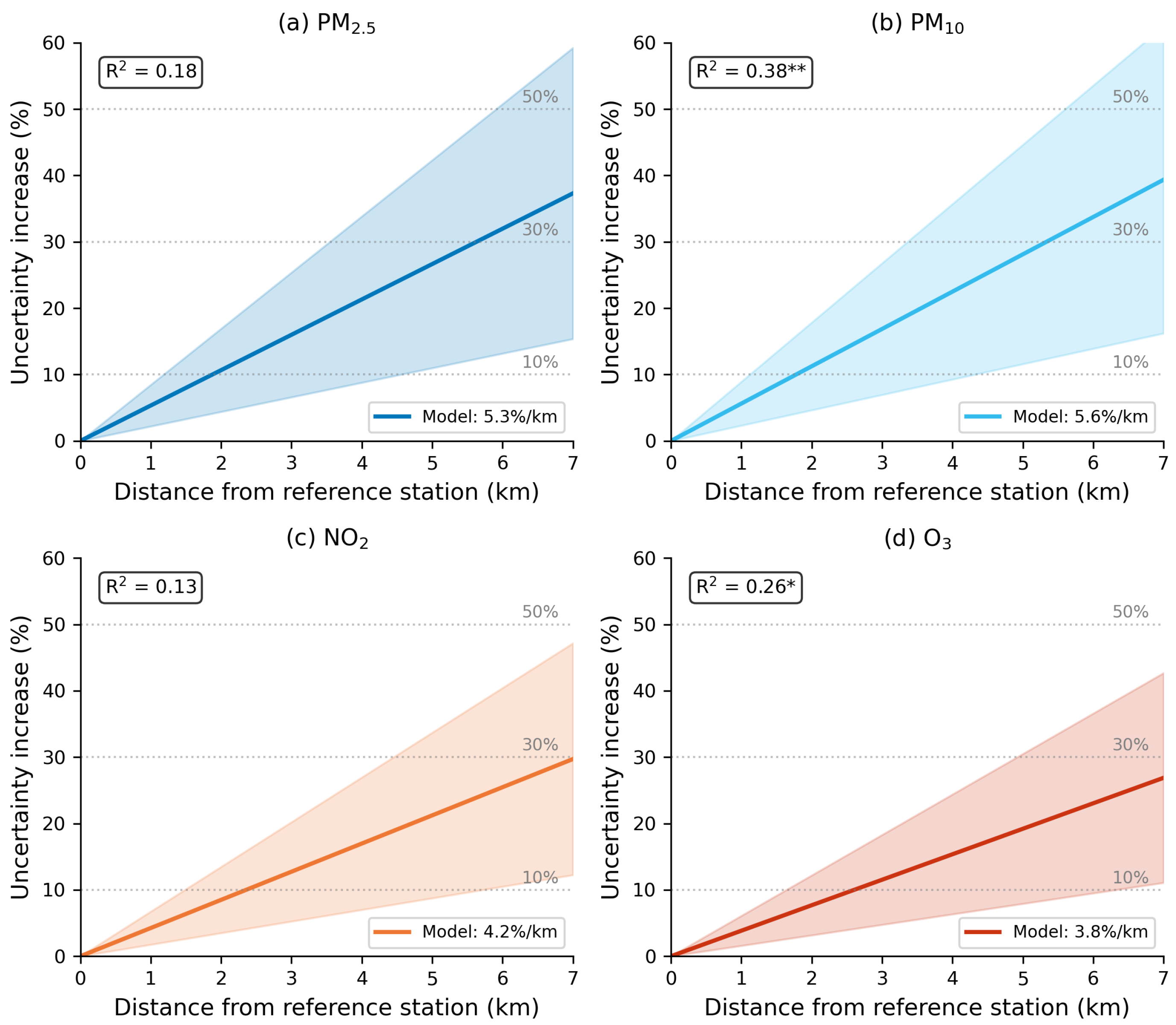
Figure 3 visualizes the uncertainty growth model, showing how prediction uncertainty increases with distance from co-location sites for each pollutant.

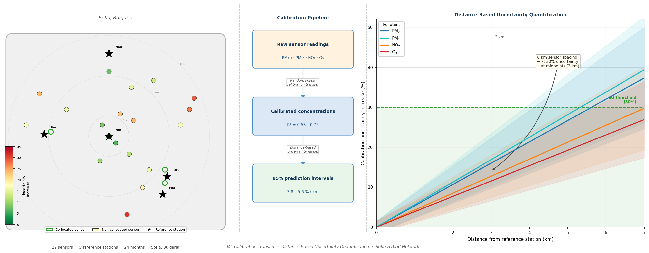
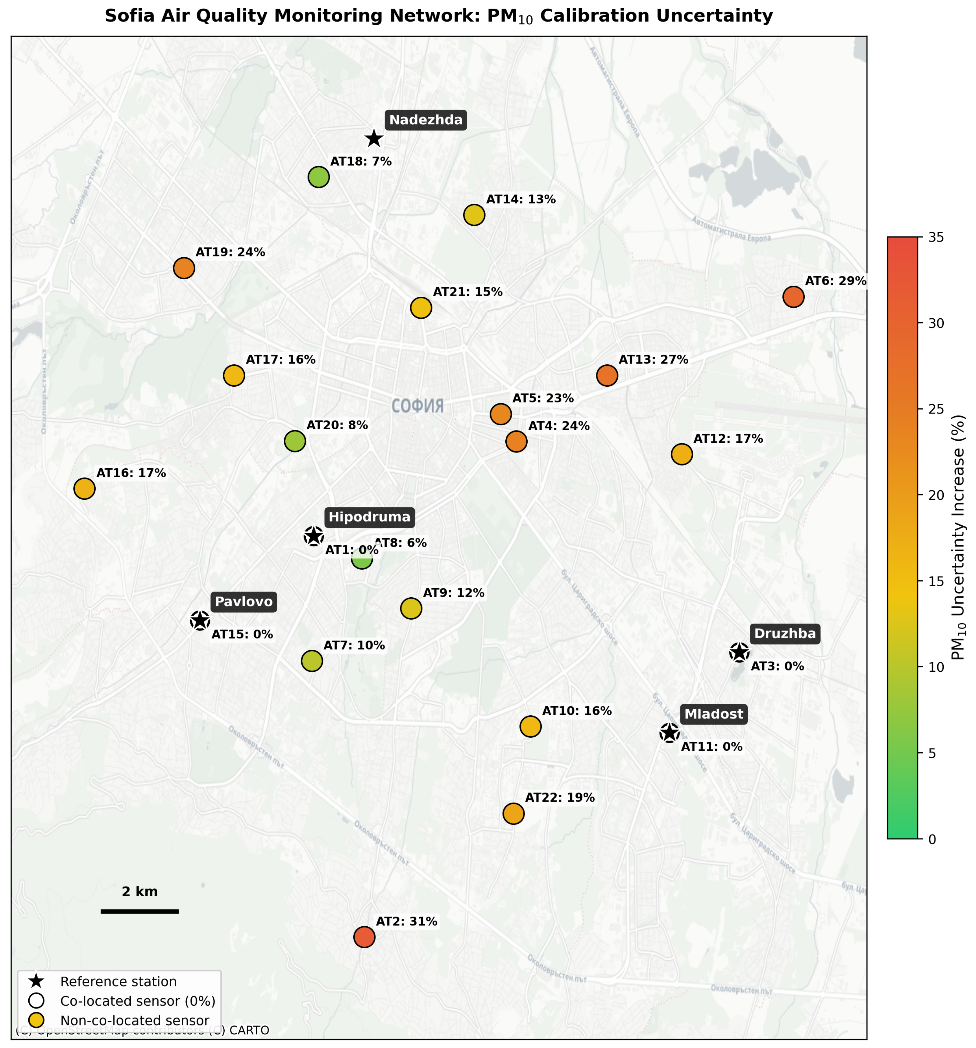
Figure 4 illustrates the spatial distribution of monitoring stations across Sofia and the predicted PM₁₀ calibration uncertainty for each non-co-located sensor. We present PM₁₀ because it exhibits the highest uncertainty growth rate (5.62%/km) among the pollutants with statistically significant distance effects, representing the most conservative (worst-case) scenario for network planning. The map demonstrates the practical application of the uncertainty framework: sensors near reference stations (e.g., AT8 at 6% uncertainty) can provide reliable, calibrated measurements, while sensors at the network periphery (e.g., AT2 at 31% uncertainty) require more cautious interpretation.

The modest uncertainty growth rates, all below 6% per kilometer, have direct implications for practical network design. At 6 km spacing between co-location sites, sensors positioned at the network midpoint (3 km from the nearest reference station) experience less than 30% uncertainty increase relative to co-located sensors. This degradation remains well within acceptable bounds for indicative monitoring applications, suggesting that relatively sparse co-location infrastructure can support city-wide calibration transfer without excessive quality degradation. The stronger statistical significance for PM₁₀ and O₃ provides confidence in these design recommendations for coarse particulate and ozone monitoring, while the consistent trends for PM_2.5 and NO₂, though not statistically significant at conventional thresholds given the limited sample of 18 transfer sensors, point in the same direction.

5. Discussion

5.1. Summary of Key Findings

This study developed and validated a machine learning-based calibration transfer framework for hybrid air quality monitoring networks. Our investigation yielded three primary findings:

First, Random Forest calibration substantially outperformed Multiple Linear Regression across all pollutants ($R^2\in (0.53,0.75)$ vs. $R^2\in (0.14,0.53)$), demonstrating the value of ensemble learning for capturing non-linear sensor-environment-pollutant relationships. The performance gains were most pronounced for particulate matter (PM_2.5: 408% improvement, PM₁₀: 370% improvement).

Second, and most significantly, we quantified spatial uncertainty degradation through a distance-based framework characterized by pollutant-specific uncertainty growth rates ($\alpha$ parameters): PM₁₀ (5.62%/km), PM_2.5 (5.33%/km), NO₂ (4.24%/km), and O₃ (3.84%/km). These $\alpha$ parameters enable prediction of calibration uncertainty for sensors deployed 1–6 km from reference stations without requiring ground-truth validation.

Third, the modest uncertainty growth rates (<6%/km for all pollutants) support practical network design recommendations: co-location sites spaced 6 km apart achieve <30% uncertainty increase at network midpoints, enabling cost-effective city-wide monitoring.

5.2. Comparison with Literature

Table 5. Comparison of calibration performance with published literature.

Study	Pollutant	R2 Range	Training Data	Notes
[10]	PM2.5	0.70–0.85	Multi-site, months	Dense co-location network
[11]	PM2.5	0.65–0.80	Multi-site, year	General calibration model
This study	PM2.5	0.745	Single pair, 24 months	Limited co-location data
[10]	NO2	0.50–0.70	Multi-site, months	Electrochemical sensors
This study	NO2	0.532	4 pairs, 24 monts	Consistent with literature
[11]	O3	0.60–0.75	Multi-site, year	Temperature-corrected
This study	O3	0.745	4 pairs, 24 monts	Strong T-dependence

contextualizes our calibration performance against published studies.

Our PM_2.5 calibration ($R^2=0.745$) is notable given reliance on a single co-located training pair (Hipodruma ↔ AT1, $n=\mathrm{16,162}$), whereas benchmark studies typically employ multiple co-location sites. This suggests that the 24-month training duration compensates partially for limited spatial replication. NO₂ performance ($R^2=0.532$) aligns with the literature findings that electrochemical NO₂ sensors are more challenging to calibrate than optical PM sensors due to cross-sensitivities to O₃ and temperature.

The MobiliSense study [53] found median correlations of only from 0.21 to 0.27 between personal exposure and fixed station measurements, with slight improvement as distance to the nearest station decreased. While that study addressed a different question, comparing mobile individuals against fixed monitors rather than fixed sensors at varying distances, it reinforces the broader principle that distance from reference infrastructure degrades measurement reliability. Our $\alpha$ parameters quantify this same phenomenon for fixed sensor networks, providing the operational metrics that network planners need.

5.3. Methodological Contribution

The distance-based uncertainty quantification framework addresses a practical gap in low-cost sensor deployment. While geostatistical methods (kriging, land-use regression) quantify ambient spatial variability of pollutant concentrations [10], and personal exposure studies demonstrate distance-dependent misclassification between fixed stations and mobile individuals [53], neither approach directly addresses the operational question facing network planners: how does calibration uncertainty degrade as sensors are deployed farther from reference stations?

Prior studies of calibration transfer (Van Zoest et al. [32], Wei et al. [33], and De Vito et al. [34]) established that transferring NO₂ electrochemical sensor calibrations across locations is unreliable, but did not quantify uncertainty as a function of spatial separation, did not address optical PM sensors, and did not provide actionable network design guidance. The present work extends this body of knowledge in three respects: it covers optical PM sensors (PM_2.5, PM₁₀) alongside electrochemical gas sensors; it introduces pollutant-specific $\alpha$ parameters that convert distance into a calibration uncertainty bound; and it simultaneously captures both calibration relocation and cross-node fabrication variance within a single operational metric.

Our framework fills this gap by providing actionable $\alpha$ parameters (3.8–5.6%/km) that quantify calibration transfer uncertainty. This quantity is distinct from ambient concentration variability: it measures how much additional error is introduced by applying a calibration model developed at one location to sensors at another location, rather than how much pollutant concentrations vary spatially. These parameters enable practitioners to predict measurement reliability at any network location without requiring ground-truth validation, supporting cost-effective decisions about co-location infrastructure density. While the specific $\alpha$ values derived here are Sofia-specific, reflecting its basin topography, source mix, and climate, the methodology itself is transferable to other cities implementing hybrid monitoring networks, though local calibration studies would be required to derive city-specific uncertainty parameters.

5.4. Practical Implications

The regulatory context provides important benchmarks for evaluating this framework’s practical utility. The EU Air Quality Directive [36] specifies Data Quality Objectives for indicative measurements at $\pm 50$% uncertainty for particulate matter. Our framework achieves less than 30% uncertainty increase at network midpoints when co-location sites are spaced 6 km apart, comfortably within these indicative measurement thresholds. This positions calibrated low-cost sensor networks as viable supplements to reference monitoring for indicative air quality assessment, community awareness applications, and preliminary spatial mapping. However, they cannot replace the fixed reference stations required for regulatory compliance monitoring and enforcement actions. It is also worth noting that reference instruments themselves carry measurement uncertainty, typically 10–15% for PM analyzers, and this baseline uncertainty propagates through calibration transfer to the low-cost sensor measurements.

The economic case for hybrid networks is compelling when comparing the costs of equivalent spatial coverage. Reference-grade PM analyzers cost approximately $20,000–50,000 per station, including installation, housing, and utility connections, while low-cost sensors cost $200–500 per unit with minimal infrastructure requirements. For Sofia’s 18-sensor low-cost network, achieving equivalent spatial coverage with reference stations would require approximately $360,000 (18 stations at $20,000 minimum each), compared to approximately $10,000 for the low-cost sensors plus the co-location infrastructure already provided by existing reference stations. This represents a 36-fold cost reduction while providing roughly ten times better spatial resolution than the existing 5-station reference network alone.

The uncertainty growth parameters derived in this study enable evidence-based decisions about co-location spacing. A spacing of 2 km between co-location sites achieves less than 10% uncertainty increase at the midpoint between stations, suitable for applications requiring high confidence. Spacing of 6 km achieves less than 30% uncertainty increase, acceptable for indicative monitoring and spatial screening. For PM₁₀, NO₂, and O₃, where four co-location pairs support robust spatial cross-validation, these recommendations rest on a solid empirical foundation. The situation for PM_2.5 is more constrained because Sofia operates only a single reference station measuring fine particulate matter, and expanding PM_2.5 reference coverage should be a priority for municipalities seeking comprehensive hybrid network design.

5.5. Limitations and Future Research

Four limitations constrain our findings, each suggesting specific directions for future research.

The most significant limitation is that our uncertainty estimates at transfer sites are predicted rather than validated. The $\alpha$ parameters quantify how uncertainty grows with distance from co-location sites, but these predictions have not been empirically verified by deploying reference instruments at the transfer locations. Mobile reference campaigns offer a path forward: deploying portable reference-grade instruments at selected transfer sites (for example, at 2 km, 4 km, and 6 km from co-location stations) for one to two week intensive measurement periods could directly validate whether observed prediction errors match the uncertainty estimates our framework provides. Sofia’s Executive Environmental Agency possesses mobile monitoring capabilities that would be suitable for such validation studies.

The distance range over which our linear uncertainty growth model has been validated is limited to 1–6 km, the spatial extent of Sofia’s current sensor network. Whether uncertainty continues to grow linearly beyond this range, or instead saturates at some asymptotic level or accelerates at greater distances, remains unknown. Extended-range validation studies in larger metropolitan areas such as London, Paris, or Berlin could address this gap and determine whether the linear model requires modification for city-wide deployments spanning tens of kilometers.

The $\alpha$ values derived here reflect Sofia’s particular characteristics: a basin topography that traps pollutants, a source mix dominated by residential heating and traffic, and a continental climate with strong seasonal temperature variations. Whether these parameters generalize to other cities is an open question. Multi-city comparative studies applying identical methodology could establish whether $\alpha$ parameters cluster by city typology (basin versus coastal versus flat terrain), climate zone, or dominant pollution sources, potentially enabling transferable lookup tables that would allow network planners in new cities to estimate uncertainty growth rates without requiring local calibration studies.

The statistical significance of the distance–uncertainty relationship varies by pollutant: PM₁₀ ($p=0.007$) and O₃ ($p=0.031$) are significant at $\alpha =0.05$, while PM_2.5 ($p=0.082$) and NO₂ ($p=0.135$) are not. This disparity is primarily a power constraint rather than evidence that the distance effect is absent for the non-significant pollutants. With only $n=18$ transfer sensors spanning a 1–5.6 km distance range, the regression has limited degrees of freedom; a positive trend can exist and remain physically consistent yet fall short of conventional significance thresholds. The $\alpha$ estimates for PM_2.5 (5.33%/km) and NO₂ (4.24%/km) are quantitatively consistent with the significant PM₁₀ (5.62%/km) and O₃ (3.84%/km) values, and all four point estimates have the same sign. Practitioners should treat the PM_2.5 and NO₂ $\alpha$ values as indicative rather than prescriptive; validation with larger networks spanning wider distance ranges would narrow the confidence intervals and determine whether the linear model holds for these pollutants.

The inclusion of temporal features (hour, month, weekend indicator) in the calibration models warrants discussion in the context of spatial transfer. It has been argued that temporal features may encode location-specific emission profiles that do not generalize to other sites. We tested this directly by running leave-one-station-out spatial cross-validation with RF models both with and without temporal features (Section 4.2). Empirically, temporal features improved spatial transfer for all three pollutants in Sofia’s network. This outcome reflects the city’s relatively compact geography, where major emission sources (residential heating, traffic) follow broadly similar diurnal and seasonal rhythms across neighborhoods. In networks with greater spatial heterogeneity, for example, in cities with highly localized industrial sources, this assumption may not hold, and temporal features could introduce the location-specific bias that prior literature cautions against.

The spatial cross-validation reveals substantial station-to-station variability, with negative $R^2$ at specific held-out stations (NO₂ at Druzhba, O₃ at Hipodruma). This is a structural consequence of the small leave-one-station-out training set: with only four co-location sites, removing one leaves just three spatial training points to span Sofia’s urban variability. When the held-out station occupies a distinctive microenvironment (Druzhba’s predominantly residential NO₂ profile is not well represented by the three remaining stations, and Hipodruma’s city-center photochemical O₃ dynamics differ from those at the outer-ring stations), the calibration model lacks sufficient spatial context to generalize, producing predictions that are systematically offset from the true concentration mean. This negative $R^2$ reflects microenvironmental specificity rather than a general failure of the calibration transfer method; the positive $R^2$ values achieved when the full four-station co-location dataset is used confirm that the approach performs reliably when spatial coverage is adequate.

A further limitation concerns interferent gases. Cross-sensitivity between non-target and target species is well documented in electrochemical gas sensors: O₃ sensors are sensitive to NO₂ and vice versa. The AirThings sensors used here provide only calibrated concentration outputs through their consumer API; raw electrochemical voltages and cross-channel signals are not accessible without manufacturer cooperation. Interferent correction was therefore not possible within our framework. Calibration accuracy for NO₂ and O₃ may consequently be reduced at transfer sites where the NO₂/O₃ ratio differs substantially from co-location training conditions.

Random Forest regressors cannot extrapolate beyond the feature space seen during co-location training; however, a coverage check (Section 4.2) confirms that 99.5% of transfer-site observations lie within the training bounds, so this structural limitation has negligible practical effect in the present network. Practitioners deploying this framework in networks with substantially different pollution regimes or climatic conditions should verify that transfer-site features overlap with training-site distributions before applying the calibration.

Finally, the constraint of having only a single reference station measuring PM_2.5 in Sofia means that spatial cross-validation is impossible for this health-critical pollutant. All PM_2.5 calibration and uncertainty estimates rest on a single co-located pair, and we cannot assess how well these calibrations transfer across the city’s diverse microenvironments. Expansion of PM_2.5 reference monitoring infrastructure would enable robust spatial validation and more reliable uncertainty quantification for fine particulate matter.

6. Conclusions

This study presents a comprehensive framework for creating validated hybrid air quality monitoring networks that combine the accuracy of official reference stations with the spatial density of low-cost sensor arrays.

Random Forest calibration models achieved $R^2$ values ranging from 0.53 to 0.75 across four pollutants (PM_2.5, PM₁₀, NO₂, and O₃), representing an average improvement of 246% over Multiple Linear Regression baselines. The superior performance of ensemble methods reflects their ability to capture the non-linear relationships between sensor readings, environmental conditions, and true pollutant concentrations that linear models cannot represent.

The central methodological contribution is the empirical derivation of distance-based uncertainty growth rates. These $\alpha$ parameters quantify how calibration uncertainty increases as sensors are deployed farther from reference stations: 5.62% per kilometer for PM₁₀, 5.33% for PM_2.5, 4.24% for NO₂, and 3.84% for O₃. These parameters enable practitioners to predict measurement uncertainty at any network location without requiring ground-truth validation at each sensor site, addressing a longstanding gap in low-cost sensor deployment methodology.

The modest uncertainty growth rates translate directly into practical network design guidance. Co-location sites spaced 6 km apart achieve less than 30% uncertainty increase at network midpoints, well within acceptable bounds for indicative monitoring applications. For PM₁₀, NO₂, and O₃, where four co-location pairs support robust cross-validation, four to five strategically placed co-location sites can provide calibration anchors for a city-wide sensor network. PM_2.5 network design remains constrained by limited reference infrastructure in Sofia, highlighting the importance of expanding fine particulate monitoring capacity.

The operational demonstration of this framework, generating 1.2 million calibrated measurements for Sofia’s 18 non-co-located sensors over 24 months, each accompanied by 95% prediction intervals, establishes that hybrid networks can provide spatially dense, quality-assured air quality data at a fraction of the cost of traditional reference-station expansion. This framework offers municipalities actionable guidance for implementing cost-effective hybrid monitoring networks while maintaining the transparent quality assurance essential for scientific credibility and public trust.