Ionospheric Schumann Resonance Signal Image Recognition Model and Its Application to the Yangbi Earthquake

Abstract

The Schumann resonance (SR) signal has attracted much attention as a potential earthquake precursor indicator. To enable rapid identification of these signals from massive volumes of China Seismo-Electromagnetic Satellite (CSES) data, this paper presents a machine learning-based image recognition algorithm. Firstly, the Ultra-Low Frequency (ULF) band power spectrum data of the ionospheric electric field was standardized to enhance the visual contrast of the signal and generate a spectrogram. A small-image dataset with standardized image size and labeled positive and negative samples was constructed by cropping the original images. High-dimensional features of the image were extracted using the deep convolutional neural network VGG16 algorithm, combined with the support vector machine (SVM) algorithm to classify whether the high-dimensional data contains SR signals. The sliding window recognition algorithm is designed to process large-format power spectrum images. The results showed that this VGG16-SVM hybrid model achieved an accuracy of 95.00% on the independent small-image test set, which was superior to both pure SVM and pure VGG16 models. On the large-format image prediction set, the overall accuracy of the model is 81.48%, and the SR physical properties of the recognition signal are verified through frequency statistics. The hybrid model was applied to the SR detection and recognition of the Yangbi earthquake in Yunnan, China, and achieved ideal results. This indicates that the proposed VGG16-SVM hybrid model can quickly and effectively identify SR signals in CSES data, which has important practical value for automated electromagnetic signal analysis in seismic research.

1. Introduction

Schumann resonance (SR) is a global electromagnetic resonance phenomenon occurring within the cavity formed by the Earth’s surface and the lower ionosphere. Primarily excited by global lightning discharges, SR manifests as a series of spectral peaks in the Extremely Low Frequency (ELF) band [1,2,3]. The resonance frequencies are fundamentally determined by the dimensions and conductivity of the Earth-ionosphere cavity [3], according to the following formula:

$$f_n=\left({\displaystyle \frac{c}{2\pi a}}\right)\sqrt{n(n+1)}$$

(1)

where c denotes the speed of light, a represents the effective radius of the Earth-ionosphere resonant cavity, which can be approximated as the Earth’s radius R_E plus the effective ionospheric reflection height (h, typically on the order of 70–100 km), and n indicates the order of the resonant mode [4]. The fundamental frequency is approximately 7.8 Hz, with subsequent harmonic frequencies at approximately 13.8 Hz, 19.6 Hz, and 25.9 Hz. While traditional monitoring relies on ground-based stations, the French DEMETER satellite demonstrated that a fraction of SR energy can leak through the lower ionospheric boundary and propagate to the upper ionosphere, making it detectable by low-Earth orbit satellites [5].

Earthquakes, involving the rapid release of energy from the lithosphere, represent one of the most destructive natural disasters, posing severe threats to human society and infrastructure [6,7]. Given their immense socio-economic impact, researching preparation mechanisms and identifying precursory phenomena are of crucial scientific and practical significance [8,9,10,11]. In recent years, research on geophysical field anomalies—particularly electromagnetic perturbations within the Lithosphere–Atmosphere–Ionosphere Coupling (LAIC) framework—has advanced significantly, enhanced by satellite technology. SR has gained attention as a potential diagnostic tool for these anomalies, as variations in its parameters (frequency, amplitude, and bandwidth) can reflect perturbations in the lower ionosphere triggered by rock fracturing, fluid migration, or radon emanation during the seismogenic process [12,13].

Numerous studies have indicated that SR anomalies appear prior to strong earthquakes. For instance, a 0.5 Hz shift in the SR fundamental frequency was observed before the 1999 Chi-Chi earthquake [14], a phenomenon attributed to electron density perturbations in the ionospheric D-layer [15]. Observations of the 2004 Niigata earthquake revealed that SR anomalies exhibited high-order selectivity [16]. More recently, researchers have utilized ground-based data to confirm anomalous enhancements in the first four SR modes before the 2011 Yingjiang earthquake [17] and significant parameter variations preceding other major events in mainland China [18,19,20,21]. These studies collectively support the LAIC mechanism and highlight the potential value of SR monitoring in exploring seismic precursors [22].

The advancement of space detection technologies has opened up new avenues for investigating these SR anomalies from a global perspective. The China Seismo-Electromagnetic Satellite is designed to acquire multi-parameter data on electromagnetic fields, plasma, and high-energy particles, enabling the tracking of seismic precursors and the monitoring of space weather [23,24,25]. The onboard Electric Field Detector (EFD) captures vector electric field information from DC to 3.5 MHz [26], providing valuable data for the study of electromagnetic wave phenomena.

While satellite observations provide a global perspective for SR research, they also present significant challenges. Operating at ionospheric altitudes (CSES at approximately 507 km), satellites receive SR signals that are contaminated by spatial environmental noise and exhibit spatiotemporal inhomogeneity. In electric field data, SR signals are weak and not observable in every orbital dataset, often requiring substantial time for manual inspection and screening. To overcome the limitations of manual identification methods, this article aims to develop a model capable of identifying SR signals from power spectral density (PSD) images. Leveraging the powerful image feature extraction capability of VGG16, the model automatically learns deep visual features associated with the presence of SR signals in ultra-low frequency (ULF) power spectrograms. Combined with a SVM for efficient classification, it determines whether an input power spectrogram contains clearly distinguishable SR signal characteristics.

Section 1 describes the background of earthquake disasters, the challenges of earthquake prediction, the basic concept of SR and its potential link to seismic precursors, the challenges of satellite-based SR observation, and the limitations of current manual identification methods. Section 2 introduces the data sources and preprocessing methods, including the generation of normalized spectrograms and the construction of the training set, highlighting the bottleneck of manual screening. Section 3 and Section 4 elaborate on the adopted VGG16-SVM hybrid recognition model and its sliding window strategy for application to large-format images. The experimental results of the model are presented, including performance evaluations on the small-image test set and the large-format prediction set, along with a comparison against baseline models. Concurrently, the physical properties of the identified signals are validated through frequency statistics. Section 5 demonstrates the application of this method in analyzing SR signals for an actual seismic event, taking the Yangbi earthquake in Yunnan as a case study.

2. Data Sources and Preprocessing

This article utilizes Level 2A standard scientific data products from ULF (DC-16 Hz) electric field data acquired by the EFD onboard CSES. The dataset includes waveform and PSD data for the three electric field components—X (north–south), Y (east–west), and Z (vertical)—in the geographic coordinate system (GEO), stored in H5 format [27]. Because SR signals predominantly propagate in the transverse magnetic (TM) mode within the Earth-ionosphere waveguide, their associated electric field vectors are mainly oriented in the vertical direction [28]. Accordingly, the Z-component of the electric field, which is perpendicular to the geomagnetic field, is selected as the most appropriate parameter for subsequent analysis.

2.1. SR Data Extraction and Preprocessing

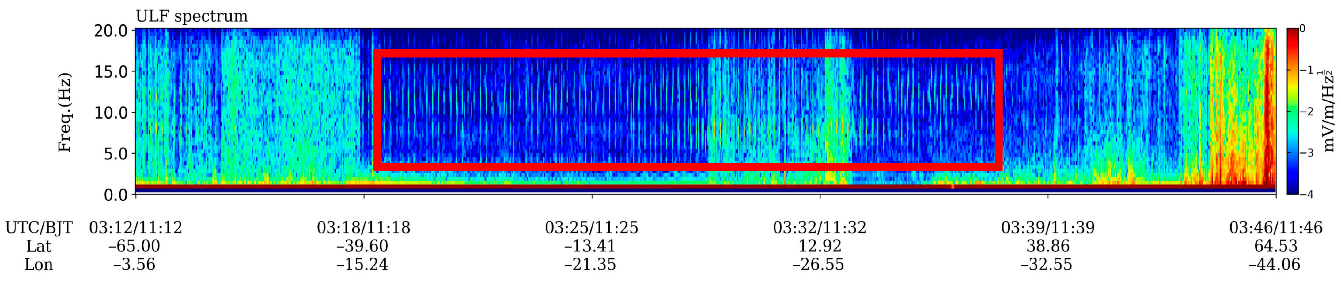
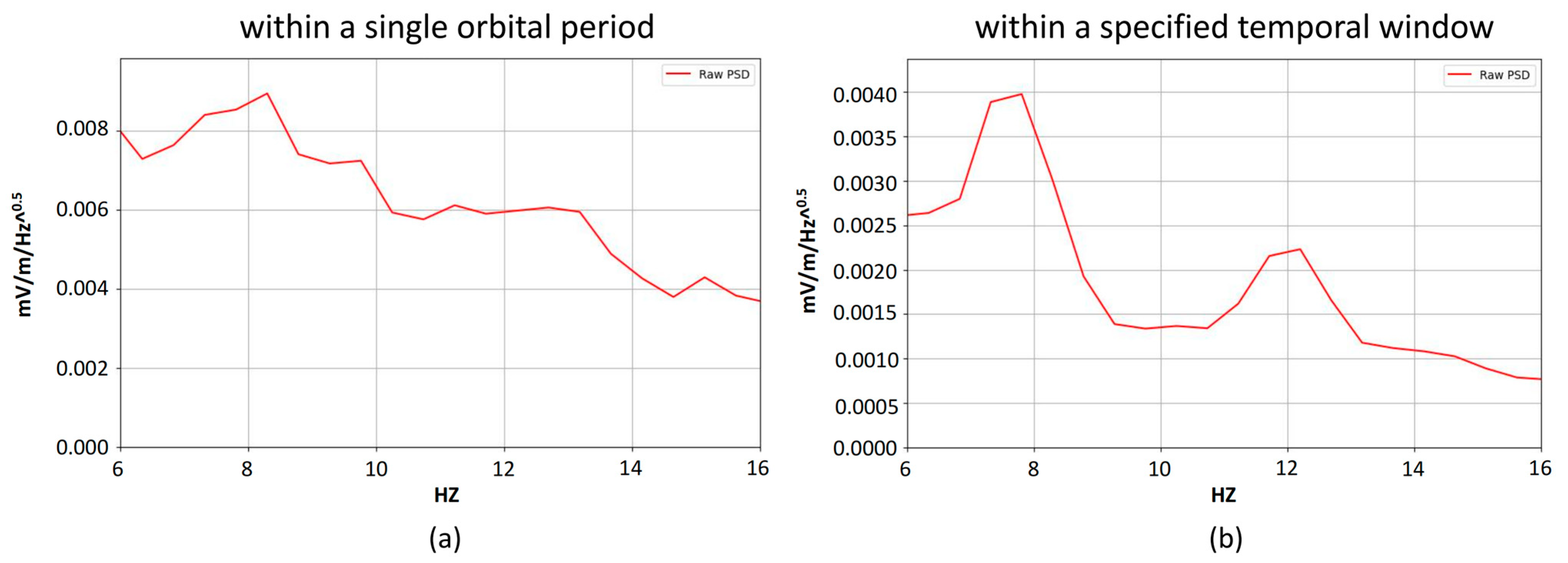
Observing SR signals at ionospheric altitudes with CSES presents unique challenges. The signals must leak from the Earth-ionosphere waveguide cavity and penetrate the ionosphere to be received by the satellite. This process can involve attenuation, frequency shifts, and the superposition of complex noise from the space plasma environment. To preliminarily assess the SR features within the data, a traditional method is to average the PSD at each frequency point over all time instances within a specific period (e.g., a single orbit’s data) to obtain an average spectrogram for that period. However, this simple averaging method is not effective for ULF data. As shown in the PSD image in Figure 1, the time interval marked by the red box contains clearly identifiable SR signals (first and second mode frequency bands), and the regions where these signals reside are precisely the targets to be detected by the model. The spectrogram of the 6–16 Hz band, obtained by directly averaging the orbital data, is presented in Figure 2a. Here, the horizontal axis represents frequency, and the vertical axis represents the PSD value. Clear SR peaks are difficult to discern, as the signal features are obscured by noise or data from non-SR periods. Conversely, if only the data within the red box in Figure 1 are extracted for analysis, an SR spectrogram with a clear dual-peak structure can be obtained, as shown in Figure 2b. Analysis of the power spectrum images indicates that clearly distinguishable SR signals—manifested as dual horizontal bands that emerge and vanish concurrently—are generally not persistent throughout an entire satellite orbit. Furthermore, the onset times and durations of prominent SR signatures vary across different orbital datasets.

Precisely because of the transient and localized nature of SR signals in satellite observations, averaging over extended time windows can substantially attenuate or even completely obscure these signals. Effectively identifying SR signatures with well-defined resonant peaks from complex power spectra, as well as determining their temporal occurrence, therefore remains a significant challenge. Consequently, there is a strong need for automated, rapid, and accurate techniques to address this problem, which constitutes the primary motivation for introducing machine learning-based methods in this study.

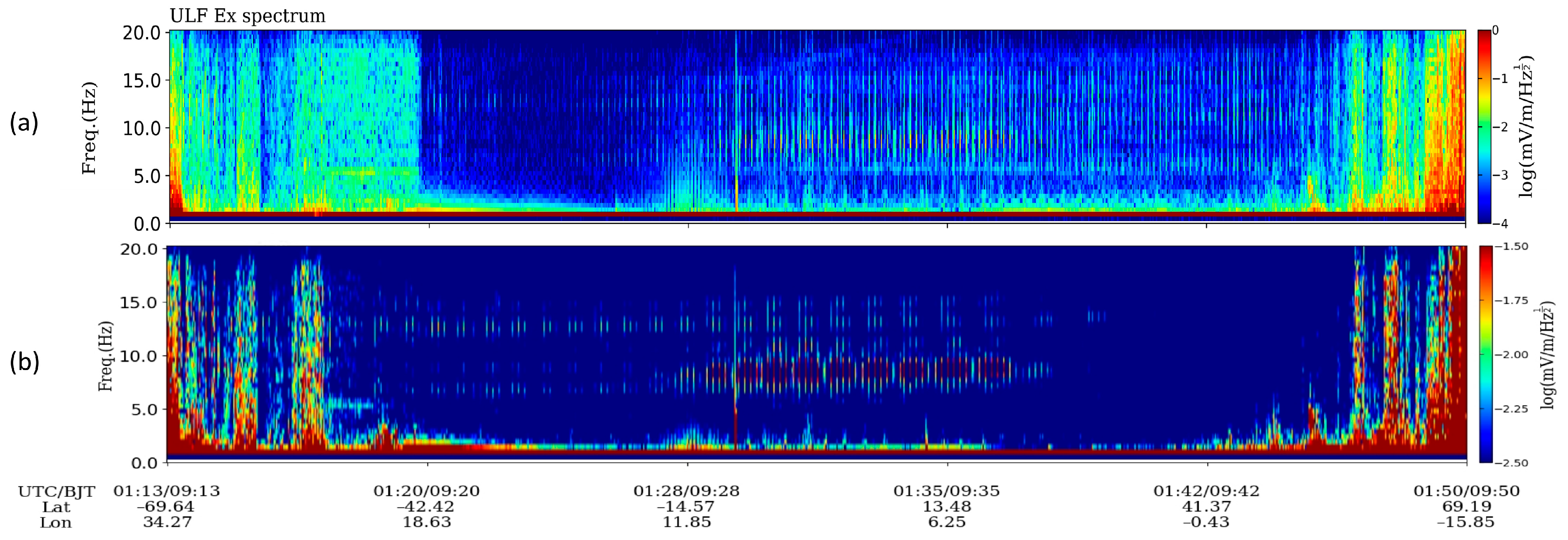
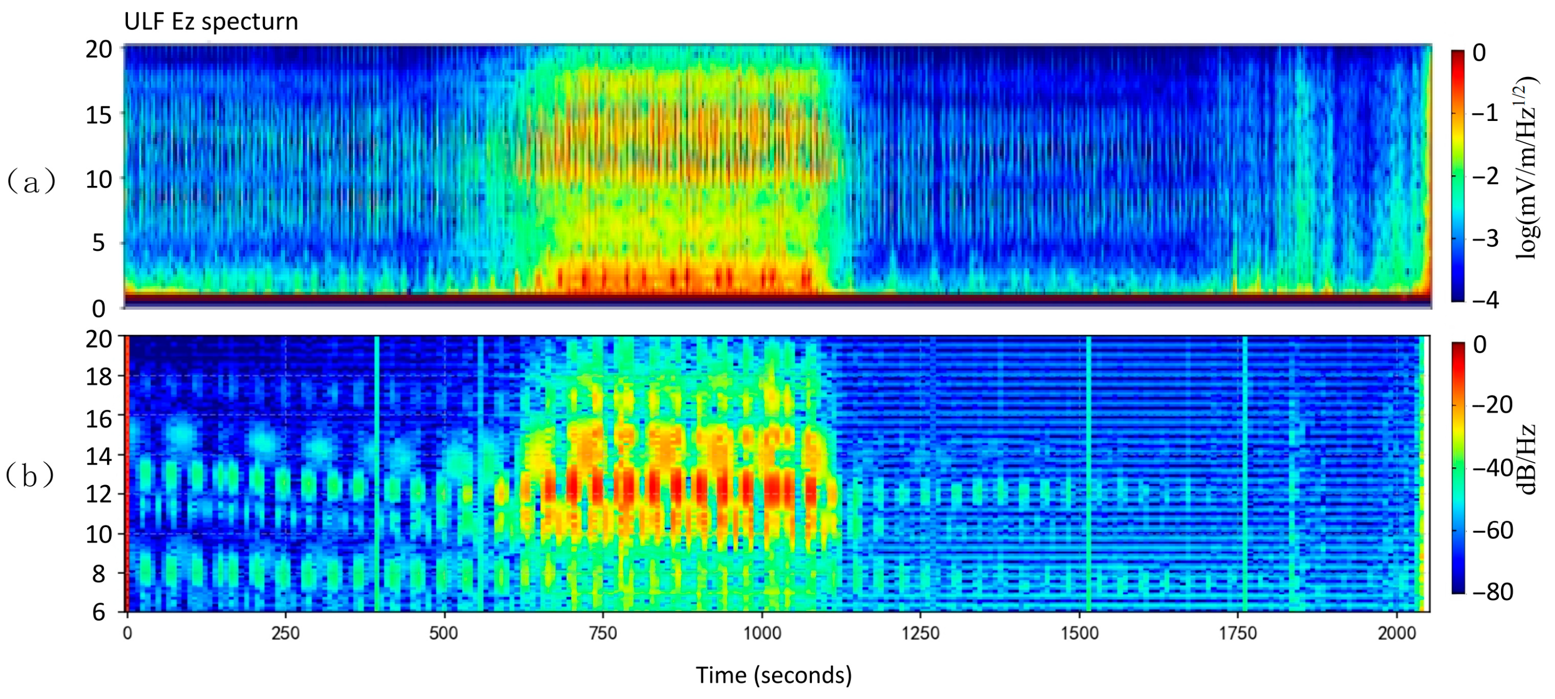
The transient and localized nature of SR signals in satellite observations often leads to substantial attenuation or complete obscuration when conventional analysis methods are applied. This limitation necessitates the development of an automated, rapid, and accurate identification technique, motivating the adoption of a machine learning-based approach. First, PSD images are regenerated by applying a base-10 logarithmic transformation to the PSD data, which compresses the dynamic range and enhances the visibility of low-intensity signal features relative to the background. Next, the ULF-band data are color-mapped using a minimum value (vmin) of −2.5 and a maximum value (vmax) of −1.5, ensuring that pixel color intensity directly reflects physical signal strength and yields a visually consistent dataset suitable for machine learning model training.

The processed images exhibit markedly enhanced contrast, rendering the characteristic horizontal banding structure of SR more distinct than in the original representations. This preprocessing strategy therefore produces a high-quality digital image dataset for subsequent feature extraction using the VGG16 network and forms the basis for training and testing the Schumann resonance identification model. Taking Orbit 22,189 on 1 February 2022, as an illustrative example, the original PSD image and the standardized image after preprocessing are presented in Figure 3a and Figure 3b, respectively.

2.2. Construction of Training Dataset

To train the proposed VGG16-SVM hybrid model, the standardized PSD spectrograms were further processed into labeled small-format images suitable for model input. Regions exhibiting clear and representative SR signal characteristics were first identified through visual inspection and subsequently cropped to generate positive sample images. Given that the original PSD spectrograms have dimensions of 1541 × 299 pixels, multiple cropping experiments were conducted to determine an optimal window size that preserves clear and continuous SR frequency bands while minimizing redundant background information. Based on these experiments, a window length of 532 pixels was selected, and all positive samples were standardized to a size of 532 × 299 pixels.

Similarly, negative samples were constructed by cropping image patches of the same dimensions from regions without distinct SR characteristics. These regions include both relatively clean background segments and segments dominated by strong background noise or non-SR interference signals. This strategy was adopted to enhance the model’s ability to distinguish true SR signals from non-SR signals and background noise.

Through this process, a binary-labeled image dataset consisting of 100 positive samples and 100 negative samples was constructed. The dataset was then divided into training and testing sets with an 8:2 ratio.

At the current stage, the labeled dataset was constructed solely based on the visual presence or absence of SR-like spectral features in the official CSES PSD images, without explicit stratification by geomagnetic activity indices (e.g., Kp or Dst). This design choice was made to ensure labeling consistency and sufficient sample size for the initial development of the proposed model.

3. Methodology for Schumann Resonance Identification

This section describes the machine learning framework employed for the automatic identification of SR signals in ULF power spectrum images. The proposed approach adopts a hybrid strategy: first, the strong automatic feature learning capability of the VGG16 network is leveraged to extract discriminative representations from the power spectrum images; subsequently, these deep features are fed into a SVM, a conventional machine learning classifier renowned for its computational efficiency and robust performance in high-dimensional feature spaces, to perform the final classification. This hybrid design aims to combine the representational strengths of deep learning with the classification advantages of SVM.

3.1. VGG16-Based Deep Feature Extraction Model

To automatically learn and extract visual features from power spectrum images that can effectively distinguish the presence or absence of SR signals, this article selected the VGG16 deep convolutional neural network model as the feature extractor. VGG16 is a widely recognized deep Convolutional Neural Network (CNN) architecture known for its elegant simplicity and remarkable effectiveness in image recognition. Proposed by the Visual Geometry Group at the University of Oxford in 2014, it represents a significant milestone in deep learning [29,30]. 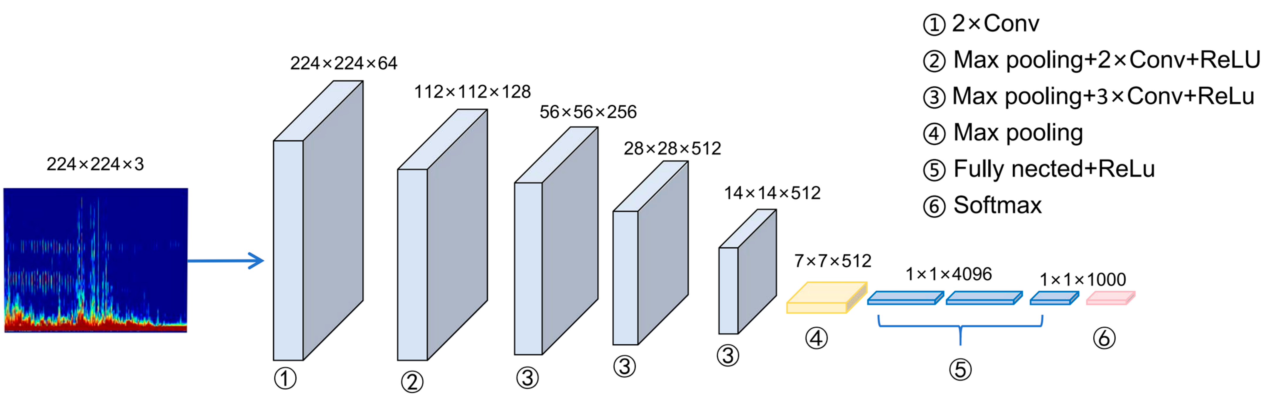The schematic diagram of the VGG16 model is shown in Figure 4. The model can be understood as a series of sophisticated, trainable filters that scan the image to identify patterns. Its core characteristic lies in the exclusive use of small-sized (3 × 3) convolutional kernels and 2 × 2 Max Pooling layers. By stacking multiple 3 × 3 convolutional layers, VGG16 can effectively increase the network depth (reaching 16 weighted layers, comprising 13 convolutional layers and 3 fully connected layers) while maintaining a smaller number of parameters, thereby enabling the learning of more complex and hierarchical image features [31]. Compared to the use of large convolutional kernels, the stacking of multiple small kernels not only reduces the number of parameters but also introduces more non-linear transformations, enhancing the model’s expressive capability. Its structure typically consists of several ‘convolutional blocks’, each containing two to three consecutive 3 × 3 convolutional layers, followed by a 2 × 2 Max Pooling layer to reduce the spatial resolution of the feature maps.

The primary reason for selecting VGG16 as the feature extractor is its robust capability for feature representation. In the context of geophysical data, the initial layers of VGG16 act as fine-grained edge detectors, capturing the “texture” of background noise and sharp transients in the spectrogram. As the data progresses through the 16 weighted layers (13 convolutional and 3 fully connected layers), these local textures are integrated into high-level semantic features—specifically, the characteristic horizontal “resonance strips” that signify SR signals. Furthermore, VGG16 offers pre-trained model weights derived from training on large natural image datasets (such as ImageNet). By loading these weights, we can exploit the models’ already learned general image feature extraction skills and transfer them to the specific spectrogram identification task. This approach significantly reduces the required data volume and training time while simultaneously enhancing model performance.

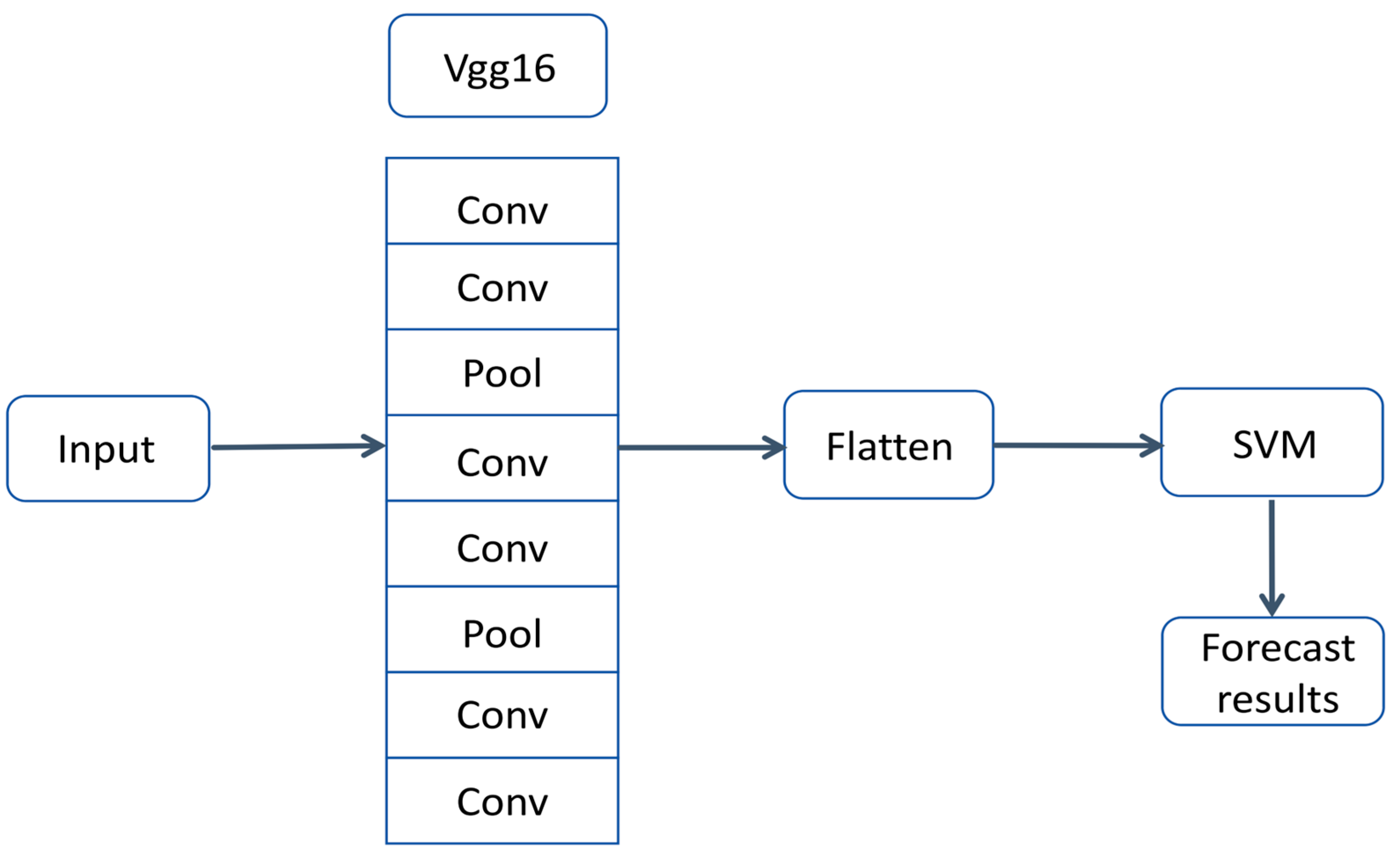
In this article, we loaded the VGG16 model, which is pre-trained on ImageNet, removed its top fully connected classification layers, and retained only its convolutional base. The VGG16 weights were set to a frozen state, utilizing the network solely as a fixed feature extraction tool. The output feature maps, generated after processing the input images through the VGG16 convolutional base, were then used as input for the subsequent SVM classifier.

3.2. SVM-Based Classification Model

After extracting deep feature vectors from the power spectrum images using the VGG16 model, a SVM is employed as the final classifier to determine whether an image contains SR signals. SVM is a supervised learning algorithm that is particularly effective in handling high-dimensional data. Its fundamental principle is to identify an optimal hyperplane in the feature space that maximizes the margin between samples of different classes, thereby enabling robust classification [32,33]. Given the high dimensionality of the feature representations produced by the VGG16 CNN, adopting an SVM as the downstream classifier constitutes a rational and effective design choice.

In this article, the input to the SVM classifier consists of high-dimensional feature vectors extracted by the VGG16 convolutional base and subsequently flattened. To effectively handle potential non-linear relationships in the feature space, the Radial Basis Function (RBF) kernel (kernel = ‘rbf’) was adopted. The key parameters for the SVM classifier were set as follows: regularization parameter C = 1, and kernel coefficient gamma = ‘scale’ (which automatically adjusts based on the number of features). During the training phase, the SVM utilized the feature vectors, labeled by class (0 for ‘no signal,’ 1 for ‘signal present’), to learn the decision boundary for model training. The overall structure diagram of the VGG16-SVM model is shown in Figure 5.

3.3. Sliding Window Identification Strategy

The VGG16–SVM model was trained using small-format image samples. In practical applications, however, full-scale standardized power spectrograms (1541 pixels in width × 299 pixels in height) must be evaluated to determine the presence of SR signals. To bridge this scale mismatch, a sliding-window detection strategy is adopted. The window dimensions are identical to those of the training images, and each windowed image patch is independently classified by the trained model. The final classification of the full spectrogram is then obtained by aggregating the predictions from all sliding windows.

To achieve a 50% overlap between consecutive windows, a stride equal to half of the window width (266 pixels) is adopted. The detection process begins at the left boundary of the spectrogram and proceeds horizontally until the sliding window extends beyond the right edge. This overlapping scheme enhances detection robustness by reducing the likelihood of missing localized SR signatures. If the predicted probability of SR presence in any window exceeds a threshold of 0.7, the entire spectrogram is classified as signal present; otherwise, it is labeled as signal absent.

4. Experimental Results and Analysis

This section systematically evaluates the performance of the proposed VGG16-SVM hybrid model for the automated identification of SR signals in CSES ULF power spectrum images. First, the quantitative evaluation results of the model on the independent small-sized image test set will be detailed, comparing its performance against the standalone SVM and VGG16 baseline models to verify the effectiveness of the hybrid approach. Subsequently, the model will be applied using the sliding window strategy to the large-format power spectrum image prediction set, and the overall identification accuracy will be calculated and analyzed in conjunction with specific prediction results tables. Furthermore, this section will present instances of the model successfully identifying images containing SR signals and their corresponding spectral features through qualitative case analysis. Finally, the model will be applied to the CSES data covering the period before and after the 2021 Yangbi M6.4 earthquake event, exploring the application potential of this automated method in real-world SR anomaly analysis for seismic events.

4.1. Performance Evaluation of VGG16-SVM on Small Image Test Set

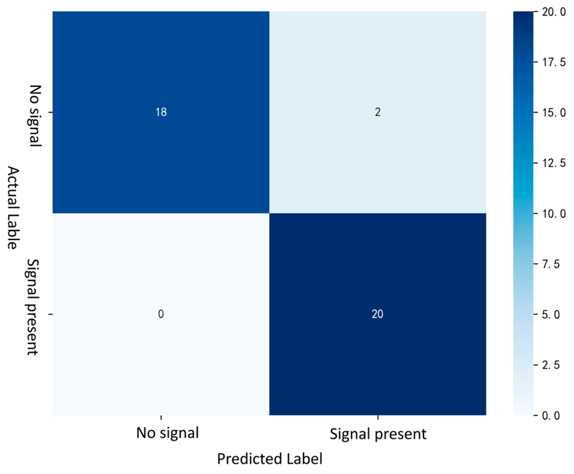
To evaluate the generalization capability of the VGG16–SVM hybrid model for SR signal identification, performance testing was conducted on a held-out small-format image test set comprising 20% of the total samples, which was not used during training. The model achieved an overall accuracy of 95.00%, indicating that the vast majority of test samples were correctly classified and demonstrating strong performance on the small-image dataset. The corresponding confusion matrix is presented in Figure 6.

Specifically, among the 20 true signal-absent samples, 18 were correctly identified, while all 20 true signal-present samples were successfully recognized. Based on these results, the precision for the signal-present class was 90.9%, with a recall of 100% and an F1-score of 95.2%, quantitatively reflecting the model’s effectiveness in detecting SR signals. The discriminative capability of the model was further evaluated using the area under the receiver operating characteristic (ROC) curve and average precision. An area under the curve (AUC) value of 0.9750, which is close to unity, indicates an excellent ability to distinguish between signal-present and signal-absent samples. Compared with the training-set AUC of 0.98, the slightly lower test-set AUC remains high, suggesting strong generalization performance without evident overfitting.

In conclusion, the VGG16-SVM hybrid model demonstrated high accuracy on the independent small-image test set, which attests to its superior discriminative capability. Its performance remained consistent with the training set results, showing no significant degradation, thereby validating the model’s effectiveness and reliability in automatically identifying SR signal features from ULF power spectrum images.

4.2. Performance Evaluation of the VGG16-SVM Model on the Large-Format Image Prediction Set

To assess the performance of the VGG16–SVM model under conditions that more closely approximate real-world applications, the sliding-window recognition strategy described above was applied to an independent large-format image prediction set. This dataset consists of 54 uncropped, standardized ULF power spectrum images, including 27 labeled as signal present and 27 labeled as signal absent. The sliding-window dimensions were set to 532 × 299 pixels with a stride of 266 pixels. If any window yielded a predicted probability exceeding the threshold of 0.7 for the signal-present class, the entire large-format image was classified as containing an SR signal.

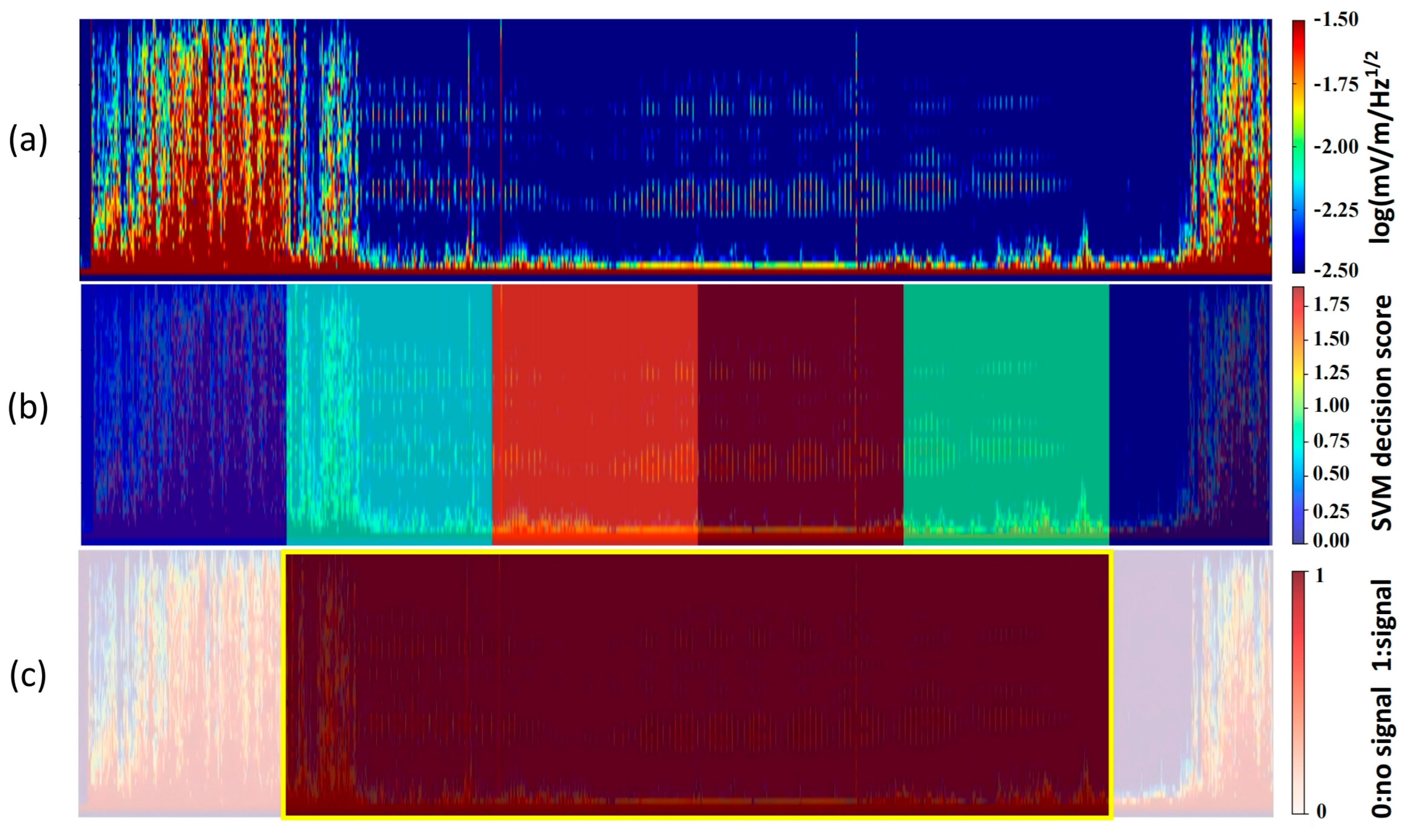
Figure 7 illustrates the implementation of the sliding-window detection strategy for a representative sample, including the original image (Figure 7a), the corresponding prediction probability heatmap (Figure 7b), and the superimposed result showing all windows in which SR signals were detected (Figure 7c). In the heatmap, color intensity reflects the model’s confidence in signal presence, with deeper red tones indicating higher confidence. When applied to the full large-format prediction set, the model correctly identified 24 of the 27 images labeled as signal present. Among the 27 signal-absent samples, 20 were correctly classified, while 7 were misclassified as containing signals. The performance metrics derived from these results are summarized in

Table 1. Performance Evaluation Results.

Category	Metric	Value
Overall Performance	Accuracy	81.48%
“No Signal” Class	Precision	0.8696
	Recall	0.7407
	F1-Score	0.8000
“Signal” Class	Precision	0.7742
	Recall	0.8889
	F1-Score	0.8276

.

As shown in Table 1, the VGG16-SVM hybrid model achieved an overall accuracy of 81.48% on the large-format prediction set, demonstrating its strong discriminative capability against complex backgrounds. For the “signal-present” class, the model attained a precision of 77.42%, a recall of 88.89%, and an F1-score of 0.8276. This performance suggests a deliberate tendency toward high recall, thereby minimizing false negatives. In contrast, for the “no signal” class, precision was higher (86.96%), albeit with a lower recall (74.07%), indicating that a non-negligible number of false positives remain.

Collectively, the high recall achieved for the signal-present class reflects the model’s strong sensitivity to target detection, while the comparatively higher precision for the signal-absent class indicates stable discriminative capability. The F1 scores, both close to 0.8, demonstrate a favorable balance in performance across the two classes. These results suggest that the VGG16–SVM model is well-suited for subsequent large-scale automatic signal recognition and screening tasks, as it preserves high detection sensitivity while maintaining a relatively low false positive rate.

4.3. Model Comparison

To validate the effectiveness of the proposed VGG16-SVM hybrid model, two baseline models were selected for comparison: a standalone SVM model and a standalone VGG16 model. The standalone SVM model classifies signals directly based on power spectral features and represents traditional machine learning approaches. In contrast, the standalone VGG16 model adopts an end-to-end convolutional neural network architecture, representing deep learning-based feature extraction methods.

4.3.1. Comparison on the Small-Image Test Set

Performance evaluation of the three models was conducted on the small-image test set, and the corresponding results are reported in

Table 2. Performance Comparison of the Three Models on the Small-Image Test Set.

Category	Metric	SVM-Only	VGG16-Only	VGG16-SVM
Overall Performance	Accuracy	85%	92.5%	95%
Confusion Matrix	TN (True Negative)	14	19	18
	FP (False Positive)	6	1	2
	FN (False Negative)	0	2	0
	TP (True Positive)	20	18	20
“No Signal” Class	Precision	100%	90.5%	100%
	Recall	70%	95%	90%
	F1-Score	82.4%	92.7%	94.7%
“Signal” Class	Precision	76.9%	94.7%	90.9%
	Recall	100%	90%	100%
	F1-Score	86.9%	92.3%	95.2%

. Overall, the proposed VGG16-SVM hybrid model achieved the best comprehensive performance, attaining the highest accuracy of 95.00%. The standalone VGG16 model also demonstrated strong performance, with an accuracy of 92.50%, whereas the standalone SVM model yielded the lowest accuracy of 85.00%. These results indicate that, for the task of identifying SR signals from power spectrum images, VGG16-based deep feature extraction plays a decisive role. Its representational capacity substantially surpasses that of the shallow image-derived features on which the standalone SVM relies. Moreover, the hybrid model achieved higher F1 scores for both the signal-present and no signal classes compared with the standalone VGG16 model. This suggests that employing an SVM classifier on top of VGG16-extracted features enables the learning of a more effective decision boundary than the fully connected layers inherent to VGG16. As a result, the hybrid approach achieves a superior balance between reducing false negatives (high recall) and limiting false positives (high precision). Collectively, these findings validate the effectiveness of the proposed hybrid model under this experimental setting.

4.3.2. Comparison on the Large-Image Prediction Set

To further assess the effectiveness of the proposed VGG16-SVM hybrid model for automatic SR signal identification, the three models were comparatively evaluated on an independent large-image prediction set. This dataset consists of 54 samples (27 signal-present and 27 no signal cases) and more closely reflects practical application scenarios. The corresponding performance metrics are reported in

Table 3. Comparison of the Three Models on the Large-Format Power Spectrum Image Prediction Set.

Category	Metric	SVM-Only	VGG16-Only	VGG16-SVM
Overall Performance	Accuracy	68.52%	79.63%	81.48%
Confusion Matrix	TN (True Negative)	11	21	20
	FP (False Positive)	16	6	7
	FN (False Negative)	1	5	3
	TP (True Positive)	26	22	24
“No Signal” Class	Precision	91.67%	80.77%	86.96%
	Recall	40.74%	77.78%	74.07%
	F1-Score	56.34%	92.7%	80%
“Signal” Class	Precision	61.9%	78.57%	77.42%
	Recall	96.3%	81.48%	88.89%
	F1-Score	75.21%	80%	82.76%

. As shown in Table 3, the VGG16-SVM hybrid model achieved the highest overall accuracy, indicating its superior comprehensive classification performance. Compared with the standalone VGG16 model, the hybrid approach substantially improved recall for the signal-present class by 7.41 percentage points while maintaining a comparable level of precision. This improvement effectively reduces the risk of missed detections, which is critical in practical SR signal identification tasks. These results demonstrate that the SVM classifier, when operating on deep features extracted by VGG16, can construct a more effective decision boundary, thereby achieving higher sensitivity and a better balance in identifying the crucial signal-present category. In contrast, the standalone SVM model exhibited a pronounced performance imbalance. Although it achieved a relatively high recall for the signal-present class, its precision was notably low (61.90%), and its ability to identify the no signal class was severely limited, with a recall of only 40.74%. This behavior suggests that, in the absence of deep feature extraction, the SVM model adopts an overly permissive decision boundary, resulting in a large number of false positives. Consequently, its performance fails to satisfy the reliability requirements of real-world applications.

In summary, the evaluation on the large-image prediction set confirms the effectiveness and superiority of the proposed VGG1-SVM hybrid model. While maintaining high precision, the model markedly enhances the detection capability for SR signals. Overall, it demonstrates superior comprehensive performance and a more favorable precision-recall balance than either the standalone VGG16 or the standalone SVM model.

5. Application Case: The 2021 Yangbi Earthquake in Yunnan

5.1. Earthquake Overview and Data Extraction

An M6.4 earthquake struck Yangbi County, Dali Prefecture, Yunnan Province, China (25.70° N, 99.87° E) on 21 May 2021, at 21:48 local time (LT), with a focal depth of approximately 8 km. The epicentral area lies within the tectonically active southern segment of the Hengduan Mountains, a region characterized by frequent seismicity and a complex crustal stress regime. To investigate variations in the atmospheric-geoelectric environment during the earthquake preparation phase, demonstrate the practical applicability of the proposed VGG16-SVM hybrid model, and perform a preliminary scientific analysis, the Yangbi earthquake is selected as a representative case study. Specifically, we analyze the temporal evolution of SR signals in orbital observation data before and after the mainshock.

Recognition was performed on ULF power spectrograms acquired from satellite orbits traversing the seismic preparation zone in May 2021. Orbits containing identifiable SR signals were selected, yielding a total of 31 qualifying orbits. From these data, the center frequencies and amplitudes of the first and second SR modes were extracted. Analysis of the temporal evolution of these parameters serves to validate the physical plausibility of the model’s recognition results and to explore their potential applicability in monitoring earthquake preparation processes.

5.2. SR Signal Recognition and Frequency Point Statistical Validation

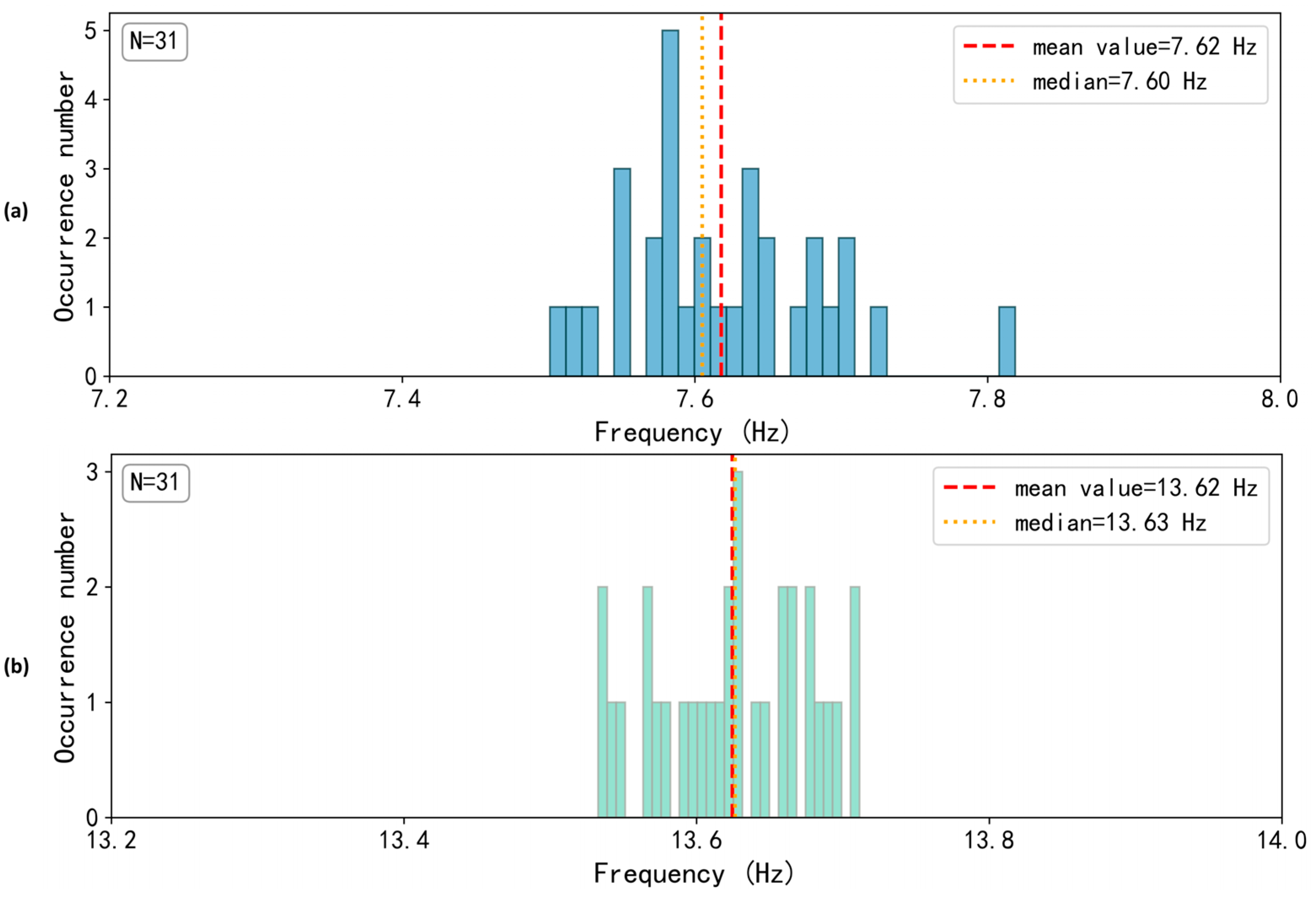
To verify the authenticity of the extracted signals, a statistical analysis was conducted on the SR parameters obtained from the pre-seismic zone in May 2021, focusing on the central frequency distributions of the first and second resonance modes. The results are presented in Figure 8. As illustrated in Figure 8, the first-mode SR frequency is predominantly concentrated between 7.4 and 8.0 Hz, with a mean value of 7.62 Hz and a median of 7.60 Hz. The second-mode frequency is distributed mainly between 13.3 and 13.8 Hz, with a mean of 13.62 Hz and a median of 13.63 Hz. The frequency ranges of both modes are consistent with the theoretical SR bands and exhibit no pronounced discrete or anomalous features, indicating that the extracted signals possess the characteristic properties of genuine SR signals.

5.3. Analysis of SR Signal Characteristics Prior to the Yangbi Earthquake

Before analyzing variations in SR parameters associated with the Yangbi earthquake, it is essential to assess concurrent space weather conditions. Geomagnetic index records indicate that global geomagnetic activity remained low throughout May 2021, with index values largely near zero and no significant geomagnetic storms observed. This relatively quiet geomagnetic environment provides a favorable baseline for detecting and interpreting SR anomalies related to earthquake preparation processes.

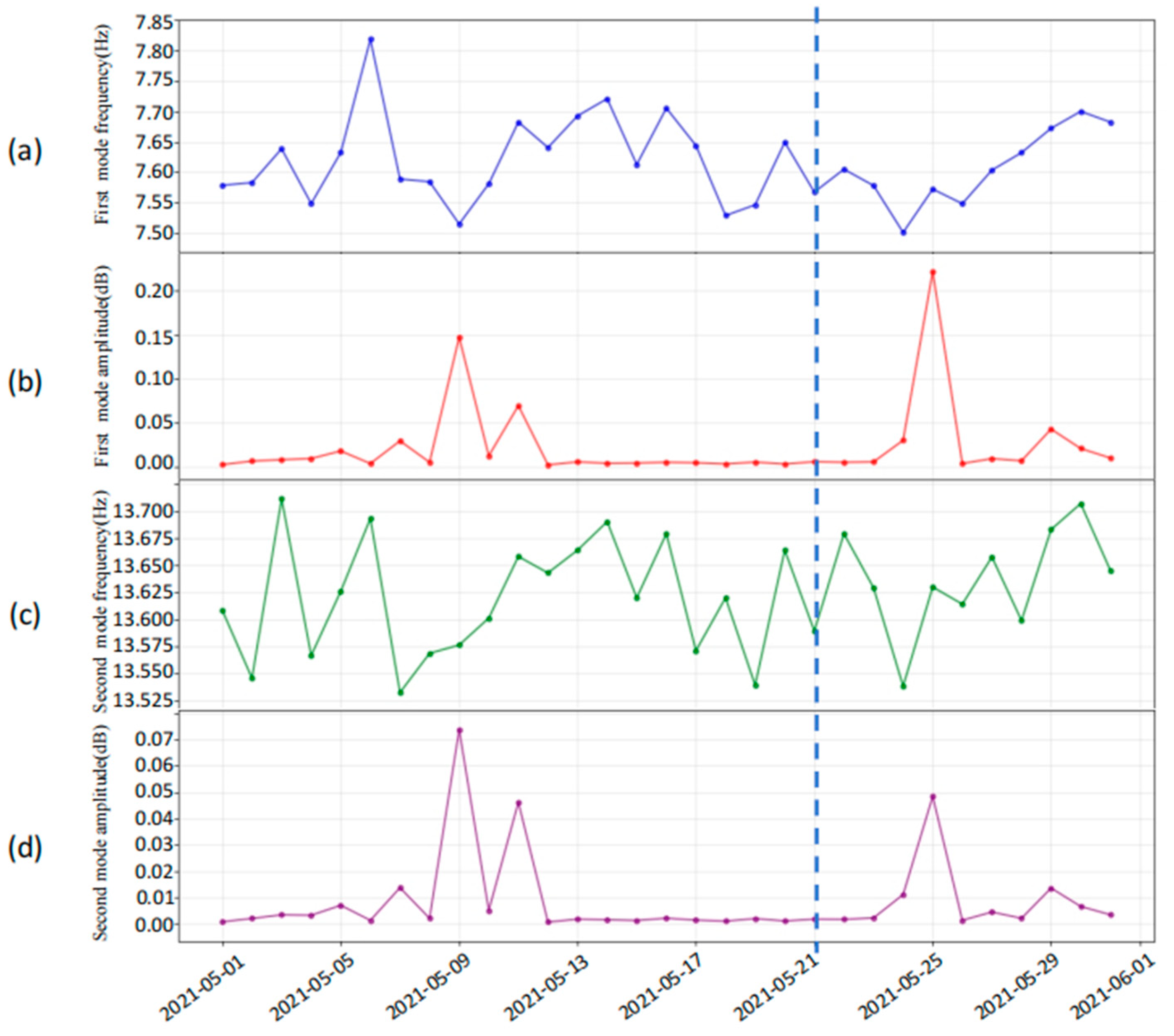
This section investigates the temporal characteristics of SR signals over the Yangbi earthquake preparation zone during May 2021, with particular emphasis on the evolution of the first- and second-mode parameters. The results are summarized in Figure 9, which presents, from top to bottom, the time series of the first-mode frequency, first-mode amplitude, second-mode frequency, and second-mode amplitude. The timing of the earthquake occurrence is indicated by vertical dashed lines.

Regarding frequency variations, the fundamental (first-order) resonant frequency remains relatively stable throughout the observation period, fluctuating primarily between 7.5 and 7.8 Hz, with an overall variation of approximately 0.3 Hz. Notably, from 9 May to 16 May (12 to 5 days before the earthquake), the first-mode frequency exhibits a gradual upward trend. The second-mode frequency ranges from 13.5 to 13.75 Hz and displays a pattern closely synchronized with the first mode, also showing an upward shift during the same period. Overall, no pronounced or persistent systematic frequency anomalies are observed in either mode. This stability suggests that the large-scale resonant cavity structure experienced no significant perturbations during the analyzed period. Nonetheless, short-term high-frequency fluctuations may result from ionospheric disturbances induced by seismic activity.

Regarding peak amplitude variations, the first- and second-mode amplitudes evolve synchronously. Both exhibit several pronounced, co-occurring enhancements prior to the earthquake—specifically on 5, 7, 9, and 11 May—with the largest increase occurring on 9 May. Following the earthquake, the amplitudes began to rise again two days later, reaching the highest values of the observation period on 25 May (four days after the mainshock). Overall, the SR signals show clear pre-earthquake amplitude perturbations, which may be associated with enhanced local ionospheric conductivity during the earthquake preparation phase. Stress accumulation in the seismogenic zone can alter surface charge distributions, generating vertical electric fields and upward currents. These processes may modify local ionospheric conductivity via mechanisms such as corona discharge and aerosol ionization. Enhanced conductivity increases the quality factor of the Earth-ionosphere resonant cavity, thereby amplifying SR amplitudes.

The post-seismic amplitude enhancement observed approximately four days after the mainshock may reflect the “post-earthquake ionospheric adjustment” mechanism described within the LAIC framework. Following the release of accumulated energy during the earthquake, the crust-atmosphere system undergoes a recovery process, during which transient adjustments in the Earth-ionosphere electric environment can induce a secondary increase in SR amplitudes.

6. Discussion

6.1. Interpretation of Frequency Shifts and Physical Origin

In the spectral analysis of CSES data, we observed that while the first SR mode is generally consistent with ground observations, the second-order peak sometimes appears around 12 Hz. While classical ground-based observations typically locate the second Schumann resonance mode near 13.8–14 Hz, frequency shifts are evident in ionospheric measurements acquired by the CSES. In particular, Qiu et al. (2024), using CSES data, reported that the SR mode frequencies observed in the ionosphere do not strictly coincide with their canonical ground-based values [34]. Therefore, the frequency ranges identified in this study are consistent with previously published CSES-based observations and should be interpreted as satellite-observed SR-like characteristics rather than as anomalies relative to ground-based SR definitions.

It should be emphasized that this study is primarily a data-driven and methodological investigation. Our core objective is to develop a robust automated identification framework to capture SR-like spectral features within the official CSES ULF power spectrum image products. At the current stage, the physical mechanisms causing this downward frequency shift are not yet fully understood. Whether these variations stem from specific LAIC processes or unique ionospheric leakage properties remains an open and continuously evolving research topic. In this context, the Yangbi earthquake case presented in this study serves only as an illustrative application of the proposed recognition method. The observed temporal variations in SR amplitudes and frequencies should be regarded as preliminary observational results rather than conclusive evidence of seismogenic precursors.

6.2. Spectral Texture and Data Processing Characteristics

The spectrograms analyzed in this study exhibit a distinct pulse-like or discrete temporal structure. These visual textures are inherent characteristics of the time-frequency discretization associated with the signal processing pipeline. Specifically, the input data utilized are official Level-2 PSD products generated via the Short-Time Fourier Transform (STFT). The resulting spectral texture is significantly influenced by the choice of STFT parameters, such as window length and overlap settings, which determine the visual manifestation of the signal in the time-frequency domain.

We compared the official products with spectrograms recomputed using different window lengths and step sizes, as illustrated in Figure 10. Figure 10a displays the original CSES Level-2 PSD product image, while Figure 10b presents a recomputed spectrogram from the same time series using a window length of 1024 points and a step size of 1024 points (i.e., no overlap). The comparison reveals that different STFT parameter configurations yield significantly distinct time-frequency textures, including the emergence or suppression of impulse-like patterns. Since the exact STFT parameters used by the CSES data provider are not publicly disclosed, we designed our VGG16-SVM model to learn from these official products directly. This approach ensures that the model can effectively recognize the stable spectral “fingerprints” of SR signals within the standardized data format used by the scientific community, providing an objective and efficient tool for massive satellite data screening.

7. Conclusions and Outlook

This study presents an automated framework for identifying ionospheric SR signals from CSES electric field data using a hybrid VGG16-SVM model. The main findings are summarized as follows:

(1)

The proposed VGG16-SVM hybrid model effectively captures the visual patterns of SR signals in power spectrum images, achieving a high accuracy of 95.00% on the small-image test set and significantly outperforming both pure SVM and pure VGG16 baselines.

(2)

With the integration of the sliding window strategy, the model enables automated detection on large-scale raw spectrograms, achieving an overall accuracy of 81.48% on an independent prediction set and demonstrating its practical effectiveness as well as its substantial improvement in data-screening efficiency.

(3)

Statistical analysis of the central frequencies of SR signals identified in the Yangbi seismic zone shows that the frequencies are concentrated within the theoretical bands of Schumann resonance. This result indicates that the proposed model predominantly detects signals consistent with established SR frequency ranges, rather than arbitrary spectral features or noise.

(4)

The model was applied to the 2021 Yangbi earthquake as a preliminary exploratory case study. While synchronous enhancements in the amplitudes of the first and second SR modes were observed prior to the event, these findings are currently considered as isolated observational instances. Further statistical analysis of a broader range of seismic and non-seismic events is required to determine the reliability and physical mechanism of such anomalies.

Although the model demonstrates strong performance, it still has limitations. The decline in accuracy on large-format images and the occurrence of false positive predictions primarily stem from information loss during sliding-window application, signal boundary truncation, and background interference. Visual patterns resembling SR signals, caused by ionospheric fluctuations or satellite platform noise, are the main sources of misidentification. Furthermore, the analysis conducted for the Yangbi earthquake is only a methodological demonstration and cannot serve as definitive evidence for earthquake precursors. Observing SR anomalies in a single seismic event is insufficient to establish a statistically reliable and universally applicable relationship between SR anomalies and seismic activity. To rigorously verify whether SR-related anomalies indeed exhibit a reliable and specific connection to stress accumulation and release processes, systematic comparative studies involving multiple earthquake events and non-seismic periods must be conducted.

In addition, a limitation of the present study is that the influence of geomagnetic activity on ULF spectral characteristics and on the robustness of the proposed identification model has not been explicitly examined. Periods of enhanced geomagnetic disturbance may alter background noise levels and spectral structures, potentially affecting the performance of automated SR recognition. A systematic assessment of model behavior under geomagnetically quiet and disturbed conditions—incorporating standard geomagnetic indices such as Kp or Dst—constitutes an important direction for future research.

Based on this, future work will focus on the following directions:

(1)

Model optimization: Explore more advanced object detection networks to overcome the inherent limitations of sliding window strategies.

(2)

Multimodal data fusion: By introducing multi-source data such as magnetic fields and plasma parameters, a more robust feature set is constructed to effectively distinguish SR signals from various background interferences and reduce false alarm rates.

(3)

Automation and Mechanism Research: Combining the automatic recognition capability of this model with the automated extraction process of SR parameters (amplitude, frequency), a large-scale SR disturbance event library is constructed to systematically study its quantitative relationship with seismic activity, ultimately promoting the automation and refinement of satellite-based seismic monitoring and electromagnetic disturbance research.

(4)

Expanding the dataset to include multiple earthquakes with different magnitudes, tectonic settings, and geographic locations, as well as carefully selected non-earthquake control periods.

(5)

Conducting statistical comparisons between seismic and non-seismic cases to quantitatively assess the reliability, repeatability, and specificity of SR anomalies potentially related to stress release.