A Review of What Can Be Learnt from Tweeks and Related Topics

Abstract

Tweeks are ELF/VLF radio signals originating from lightning discharges that exhibit dispersion due to their propagation in the Earth-ionosphere waveguide. Examples of the waveforms of tweeks and their dynamic frequency-time spectra are presented and interpreted. Tweeks observed in the daytime and night-time are compared and contrasted. Tweeks observed during a solar eclipse are also discussed, as are those due to volcanic lightning and those claimed to be recorded some hours or days before a strong earthquake. The variations of tweek occurrence with season and geomagnetic activity, and with variations of solar radiation over the 11-year solar cycle, are reviewed. Wherever possible, geophysical interpretations are discussed. Theoretical models of tweek waveforms and spectra are considered; they vary according to the lightning current model used, the distance from the source (≥1 Mm), the vertical profile of ionospheric D-region ionisation and the specific mode theory used. The simplest interpretation shows that the first-order tweek cut- off frequency ~1.8 kHz is explained as reflection by the ionosphere at a height of ~83 km where the electron density is ~27 × 10⁶ m⁻³. More complex interpretations are also reviewed and compared with electron density observations made by rockets and with profiles given by lower ionospheric models such as the International Reference Ionosphere or the Faraday International Reference Ionosphere.

1. Introduction

Atmospherics, abbreviated as sferics, are broadband radio signals in the audio frequency range; they are the electromagnetic radiation arising from the impulsive currents of vertical or nearly vertical cloud-to-ground, return stroke, lightning discharges. Tweeks are ELF/VLF (3 Hz to 3 kHz/3 to 30 kHz) radio signals produced by such lightning discharges whose broadband spectrum has been modified by propagation over some thousands of km in the Earth-ionosphere waveguide. When played through a loudspeaker, they are termed “static” and they sound like clicks or crackles. Burton and Boardman [1] introduced the term “tweeks” for these musical atmospherics, which are short damped oscillations that normally occur during twilight or at night. At sunset their frequency is about 2.3 kHz, reducing gradually to 1.8 kHz over 2.5 h [1]. Further, Burton and Boardman [1] noted that they appear “to result from multiple reflections of a static impulse between the Earth’s surface and a reflecting layer located in the upper atmosphere”. Burton and Boardman [2] showed in their Figure 3 the waveform of two such musical atmospherics given the onomatopoeic name of tweeks, and in Figure 4 their spectrograms, falling from 4 kHz to ~1.8 kHz in ~40 ms. They ascribed this characteristic spectral shape to propagation in the waveguide over a distance ~1800 km. They also noted other “swishing” sounds, falling in frequency; these are now termed whistlers (Helliwell [3]).

The group velocity of the lightning-generated impulse is reduced to zero at the waveguide cut-off frequency (f_cm = mc/2h, where m is an integer, c is the velocity of light in free space, and h is the height of the D-region of the ionosphere above the Earth; f_c ~1.8 kHz, so that h ~83 km, and assuming that the refractive index of the air in the waveguide is unity). The signal at, and just above, these cut-off frequencies is dispersed and lasts for some 30 or 40 ms. At frequencies just below f_c, for m = 1, the signal is strongly attenuated.

The vertical electric field and/or the horizontal magnetic fields (N-S or E-W) of the propagating wave is measured. Other examples of the waveforms of tweeks have been published in Figure 2 of Yano et al. [4], with m = 7, in Figure 1 of Shvets [5] and in Figure 6 of Santolik and Kolmasova [6]. They all show nearly sinusoidal oscillations at ~1.8 kHz. Shvets [5] calculated instantaneous complex dynamic spectra using a 280-point fast Fourier transform (FFT) algorithm; his Figures 2 and 3 clearly show the dispersed signals for m = 1 and 2, which last for 26 ms. The polarisation of the waves was also analysed. Because of the presence of the horizontal component of the Earth’s magnetic field, the parameters for East to West propagation differ from those for West to East propagation (Shvets and Hayakawa [7]); for East to West propagating waves, the attenuation near the cut-off frequency is less than for West to East propagation. This is because, in the ionospheric plasma, which is a bi-refringent medium, both ordinary (O) and extraordinary (X) waves can propagate. Helliwell [3], Ratcliffe [8] and Budden [9] show that the refractive index n of a collision-less plasma is given by magnetoionic theory as

n² = 1 − ω_P²/ω(ω ± ω_B)

(1)

where ω_P is the angular plasma frequency, (N_ee²/ε₀m_e)^0.5, and ω_B is the angular electron cyclotron frequency, eB/m_e, with N being the electron number density (in m⁻³), e the magnitude of the charge on the electron, of mass m_e, ε₀ the permittivity of free space, B the geomagnetic field flux density, and ω = 2πf. For the lower ionosphere, the plasma frequency f_P << 1 MHz; in the F2 region of the ionosphere, f_P ≥ 10 MHz. The electron gyrofrequency f_B ~1.1 MHz in the lower ionosphere at the geomagnetic equator; it increases with increasing latitude away from the geomagnetic equator.

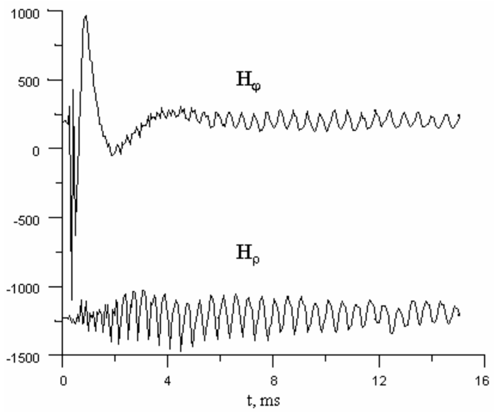
Figure 1 presents an example of a tweek waveform showing two orthogonal magnetic field components, taken from [5]. The first 2 ms correspond to the “head” and the “tail” is seen from 4 to 14 ms; the frequency of the “tail” is ~2 kHz. Shvets [5] considers that the latter (“tail”) portion of the tweek is formed by an extraordinary wave (X-mode) that has reflected from the ionosphere. Because the square of the refractive index for the ordinary wave (O-mode) is always positive (and can be ≫ 1), taking the negative sign in the denominator of Equation (1), this wave can penetrate up into the ionosphere. This leads to the right-handed polarised whistler mode propagation through a plasma in the direction of the geomagnetic field, in which the wave electric and magnetic fields are perpendicular to the geomagnetic field and rotate in the same direction as electrons rotate about the geomagnetic field in their cyclotron motion [3]. On the other hand, for the X-mode (left-handed circular polarisation [8,10]), with the positive sign in the denominator of Equation (1), the refractive index decreases with increasing height as n increases until a height is reached where the refractive index becomes zero and the wave is reflected. Using Equation (1), for kHz signals this occurs when

ω_P² = ω(ω + ω_B) ≅ ω × ω_B

(2)

or

f_P² ≅ f_c1 × f_B

(3)

Inserting typical numerical values for low magnetic latitudes, f_c1 = 1.8 × 10³ s⁻¹ and f_B = 1.2 × 10⁶ s⁻¹, we find that f_P² = 21.6 × 10⁸ s⁻², so that f_P = 4.65 × 10⁴ s⁻¹. This means that the electron density N_eR at the reflection level is (4π² ε₀m_e/e²) 21.6 × 10⁸ = 26.8 × 10⁶ m⁻³, or ~27 × 10⁶ m⁻³ to two significant figures. According to Shvets and Hayakawa [7], this corresponds to a reflection height h_R1 of ~88 km. For higher-order modes, the reflection height will be higher up.

The electrical conductivity of the lower ionosphere [3] is given by

σ = N_ee²/m_eν_en

(4)

where ν_en is the electron-neutral particle collision frequency. A night-time vertical profile of σ has been presented by Kudintseva et al. [11], based on the profile of Rycroft et al. [12]. The conductivity is approximately 3 × 10⁻⁶ S/m at a height of 88 km. It is important to note that σ increases rapidly with increasing altitude in the low ionosphere because N_e increases and ν_en decreases, being proportional to the density of neutral atmospheric particles N_n, which falls off with increasing height h according to exp(-h/H), where the neutral gas scale height H is given by

H = kT_n/m_ng

(5)

with k being Boltzmann’s constant, T_n the neutral gas temperature, m_n the mass of the neutral atoms or molecules and g the acceleration due to gravity.

Good examples of the dispersed spectra of observed tweeks at ~1.8 and 3.6 kHz are presented in Figure 1 of Singh and Singh [13], Figure 1 of Ohya et al. [14,15], Figure 1 of Kumar et al. [16], Figure 1 of Maurya et al. [17,18,19], Figure 2 of Shvets et al. [20], Figures 1 and 2 of Ammar and Ghalila [21], and Figure 3 of Maslej-Krešňáková et al. [22]. Papers [4,5,6,7,13,14,15,16,17,18,19,20,21,22] also provide references to useful earlier papers. The cut-off frequencies of tweeks can certainly be measured to the nearest 0.1 kHz, and even to the nearest 0.03 kHz (30 Hz).

In this paper, I attempt to review the literature on tweeks that has been published in the last 25 years. I explore how tweeks, particularly their m = 1 cut-off frequencies, vary with local time, occur during a solar eclipse, may be generated by volcanic lightning, may be changed by what happens on the Earth’s surface and in the atmosphere before large earthquakes, and vary with season, geomagnetic activity, and the solar cycle. Finally, I consider theoretically how tweeks are produced as the impulsive radio energy from a lightning discharge propagates over thousands of km (i.e., Mm) between thunderstorms and VLF radio receivers in the waveguide formed between the very good conducting Earth and the good conducting D-region of the ionosphere.

2. Variation of Tweek Characteristics with Local Time and Geomagnetic Latitude

Tweeks occur during the night and at sunset times, as first reported by Burton and Boardman [1,2]. Here the properties of tweeks as reported in the scientific literature since the year 2000 are presented, starting with the earlier papers and those considering tweeks recorded at lower latitude stations.

Tweeks were observed at Suva (geomagnetic latitude −22.1°, dipole model, using the British Geological Survey geomagnetic coordinate calculator based upon [23]), on the island of Fiji, by Kumar et al. [24]. They deduced that, between 21 and 03 Local Time (LT), the electron density N_eR at the reflection level was between 29 and 170 × 10⁶ m⁻³ at 83 to 87 km altitude, increasing as the order of the waveguide mode m increased up to 6. Their Figure 5 showed good agreement between the lower ionosphere profile deduced from tweeks and the profile modelled by the International Reference Ionosphere (IRI) [25] for that location and time of the solar cycle. Kishore et al. [26] extended this work, finding that most (62%) tweeks led to N_eR = 28 × 10⁶ m⁻³ at h_R1 = 84 ± 1 km.

Saini and Gwal [27], from recordings of rather short duration tweeks made during the latter part of the austral summer in 2003 and 2005 at the Indian Antarctic station, Maitri (geomagnetic latitude −67.7° [23]), deduced that h_R1 values were between 64 and 79 km; they increased from rather low heights as the day length decreased from January to March. The source of the tweeks was lightning at equatorial latitudes, and propagation from there in the Earth-ionosphere waveguide was partly in sunlight and mostly over the good conducting ocean [27].

For tweeks recorded at Allahabad, India (geomagnetic latitude +16.1° [23]), Maurya et al. [18] found that in four winter months most (67%) occurred between 21 and 03 LT. Tweek occurrence was only ~18% in winter, 19% in equinoctial months, and 63% in summer. About 93% of the tweeks propagated in the Earth-ionosphere waveguide a distance of between 2000 and 8000 km. For the annual average, h_R1 was ~86 km at 21 LT, rising to ~90 km at local midnight. Maurya et al. [19] showed that N_eR was between 22 × 10⁶ m⁻³ and 24 × 10⁶ m⁻³ and that the D-region profile obtained agreed well with rocket observations made in India and reasonably well with IRI profiles [25]. Their Figure 6 clearly shows that the log N_eR1 profile is essentially linear with height, whereas the IRI profile is distinctly curved.

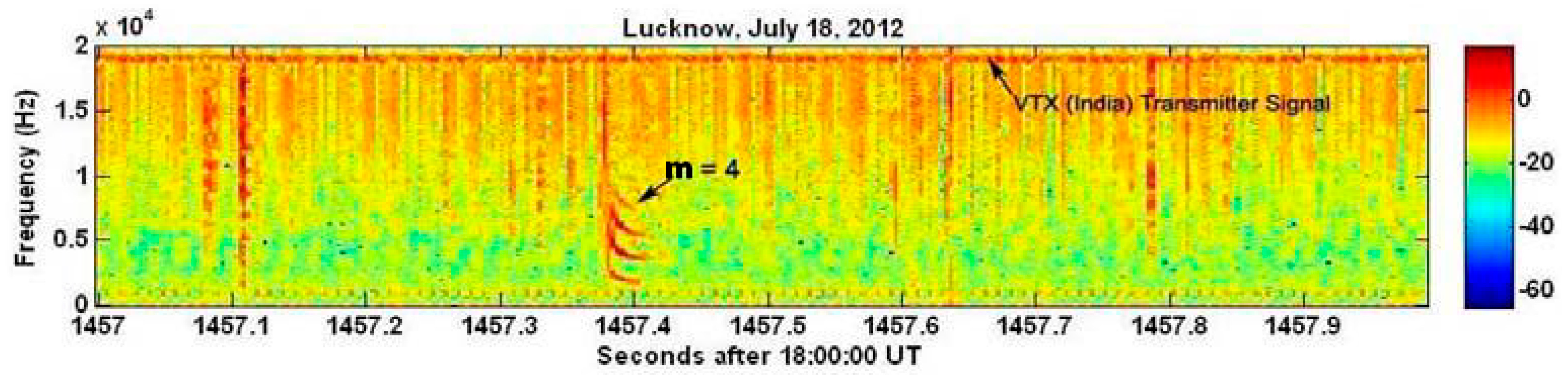
Singh et al. [28,29] presented some spectrograms of tweeks observed at Lucknow, India (geomagnetic latitude +17.6° [23]); Figure 2 is an example, up to 20 kHz, of a record lasting 1 s [28]. They interpreted such spectrograms using Equation (3), finding that N_eR1 was 26 × 10⁶ m⁻³ and h_R1 was 81 km. Tiwari et al. [30] recently reported on night-time tweeks recorded at Varanasi, India (dipole geomagnetic latitude +16.8° [23]) during 2018 and 2019. They were interpreted according to Equation (3), the electron density at the reflection level being 22 to 25 × 10⁶ m⁻³, with the reflection height generally being between 83 and 90 km for mode 1.

Tan et al. [31] showed that tweek occurrence in Vietnam is about 51% during summer, 22% during winter, and 27% during the equinoxes. Tan et al. [32] found that in 2013 the tweek reflection level electron density varied from 25 to 190 × 10⁶ m⁻³, corresponding to tweeks with m = 1 to 8 at reflection heights from 82.2 to 86.5 km. Tan et al. [33] reported that in Vietnam (geomagnetic latitude +3.4° [23]) N_eR1 values ranged between 25 × 10⁶ m⁻³ and 27 × 10⁶ m⁻³, being largest in winter, and with h_R1 ~80 km in winter, almost 82 km in the equinoxes, and ~85 km in summer; N_eR1 values decreased through the night during all seasons. Observations made at a Japanese station, Kagoshima (geomagnetic latitude +23.0° [23]), surprisingly showed that N_eR1 increased during the night, from 20 LT to 04 LT, in both summer and winter. The mean electron density of 25.0 × 10⁶ m⁻³ observed during 2014 in Vietnam, close to the magnetic equator, was 2.1 × 10⁶ m⁻³ larger than in Japan (22.9 × 10⁶ m⁻³). This is because the peak rate of electron production in a “Chapman” type of ionospheric layer [8] is proportional to cos χ, where χ is the solar zenith angle. Near the equator, cos χ is just <1, and it is 0.85 at Kagoshima. The seasonal variations of N_R1 could be caused by the geocoronal Lyman α intensity enhancement [34] and by seasonal variations of the density of nitric oxide molecules at ~80 km altitude [33].

From observations made with an AWESOME VLF radio receiver in Malaysia (geomagnetic latitude −6.7° [23]), Shariff et al. [35] estimated that the ionospheric electron density varies from 24 to 28 × 10⁶ m⁻³ at an altitude of 73 to 87 km during the local night. Using local winter (June 2010) recordings from Palmer station, Antarctica (geomagnetic latitude −55.7° [23]), Shariff et al. [36] reported that, for m = 1 or 2, N_eR was between 25 and 33 × 10⁶ m⁻³, with h_R being from 65 to 82 km. Mention was made of tweeks in Cohen et al. [37], where the performance of the AWESOME receiver system was fully detailed.

Using observations made in Tunisia (geomagnetic latitude +37.1° [23]), Ammar and Ghalila [21] deduced that N_eR was 25 × 10⁶ m⁻³ for m = 1 and 145 × 10⁶ m⁻³ for m = 6, with h_R ranging from 77 km to 95 km. Agreement with the IRI model was found [25]. On two days in October 2015, h_R increased during the night, from 80 km at 18 UT to 84 km at 03 UT. The lightning sources were found to be from 500 km to 5000 km from the observing station.

Ostapenko et al. [38] showed that tweeks recorded at 23 UT on 6 October 2005 in Northern Finland (geomagnetic latitude +64.8° [23], in the auroral zone) were purely left-hand circularly polarised at 1.6 to 1.8 kHz, the cut-off frequency f_c1 of the m = 1 mode. This frequency being lower than that usually observed at lower latitudes could be explained, using Equation (3), by f_B being higher or by a higher h_R1 at that time when the three-hourly magnetic index a_p of geomagnetic activity was only 2.

With a vertical electric field and two orthogonal magnetic field antennas, recordings were made of tweeks early in 2019 at the Ukrainian station Akademik Vernadsky on the Antarctic peninsula (formerly the British station, Faraday, geomagnetic latitude −56.2° [23]) by Shvets et al. [20]. Disagreeing with their earlier result [7], they found that “with an increase in the mode number and, accordingly, the frequency of the incident wave, the effective height of the waveguide decreases. That is explained by a decrease in the penetration depth of the low-frequency wave into the ionosphere with increasing frequency”. Their theoretical treatment of waveguide modes is based on Shvets et al. [39], which is a more accurate interpretation of the experimental observations than the simple reflection condition (Equation (3)). They showed that the amplitude spectrum of a tweek exhibits a complicated structure resulting from the interference between different waveguide modes (for either parallel plate or spherical waveguides); it also depends on the distance from the source. For the specific tweek shown in Figure 2 [20], the cut-off frequencies of the two waveguide modes were 1.661 kHz and 3.355 kHz, and the source–observer distance was 5325 km; the source azimuth was 41° measured from geographic North. The height of the lower ionosphere h_R1 was found to be 87.3 km, where the electron density was 2740 × 10⁶ m⁻³, which is about a hundred times larger than values quoted earlier in this paper [7]. The IRI profiles [25] seen in Figure 6 of [19] show that such a difference could be accounted for by the IRI profile being 4 km higher than the value of h_R1 obtained by using Equation (3).

For the night of 28 to 29 March 2019, tweeks arose from thunderstorms (a) in the Atlantic Ocean at a distance of 5500 km, (b) near the southern tip of Africa at a distance of 7200 km, and (c) a relatively weak centre to the south of the mouth of the River Plate in South America, at a distance of ~2900 km from the Antarctic observatory [20]. Variations with UT of the ionospheric parameters along the three propagation paths were deduced. The tweeks arrived in the time interval between sunset at the observatory and sunrise at the thunderstorm centre near Africa; the South American east coast centre was active all through the night. Lightning discharges were registered at distances from 2 Mm to about 10 Mm, covering almost the entire South American continent (where f_B values are unusually low due to the South Atlantic Geomagnetic Anomaly), southern Africa, and the Gulf of Guinea.

Shvets and Gorishnya [40] described a technique for distance finding to the sources of the lightning discharges concurrently with obtaining the height of the ionosphere. The approach used the interference between different waveguide modes in the amplitude spectra of tweeks. The source–observer distances were found to range from 500 to 4000 km for waveforms recorded aboard the research ship Academician Vernadsky in the Atlantic and Indian Oceans from February to April 1991. The variations of ionosphere height were 5 to 6 km during the night, rising as the solar zenith angle increases from 105° to 167°, and having changes of 2 to 3 km with season. The reflection height was found to be a few km higher than given by the IRI [25]. The “head” portion of the tweek is linearly polarised whereas the “tail” part is almost circularly polarised. Gorishnya [41] has shown that the calculated values of N_R lie in the range from several tens to several thousand times 10⁶ m⁻³ at radio wave reflection heights from 80 to 100 km. These parameters are in good agreement with the results of rocket measurements of electron density profiles (Friedrich et al. [42]), which exhibit a very steep increase in electron concentration from 10⁶ to ~10⁹ m⁻³ in the altitude range from 80 to 90 km, combined with much smaller variations at higher altitudes.

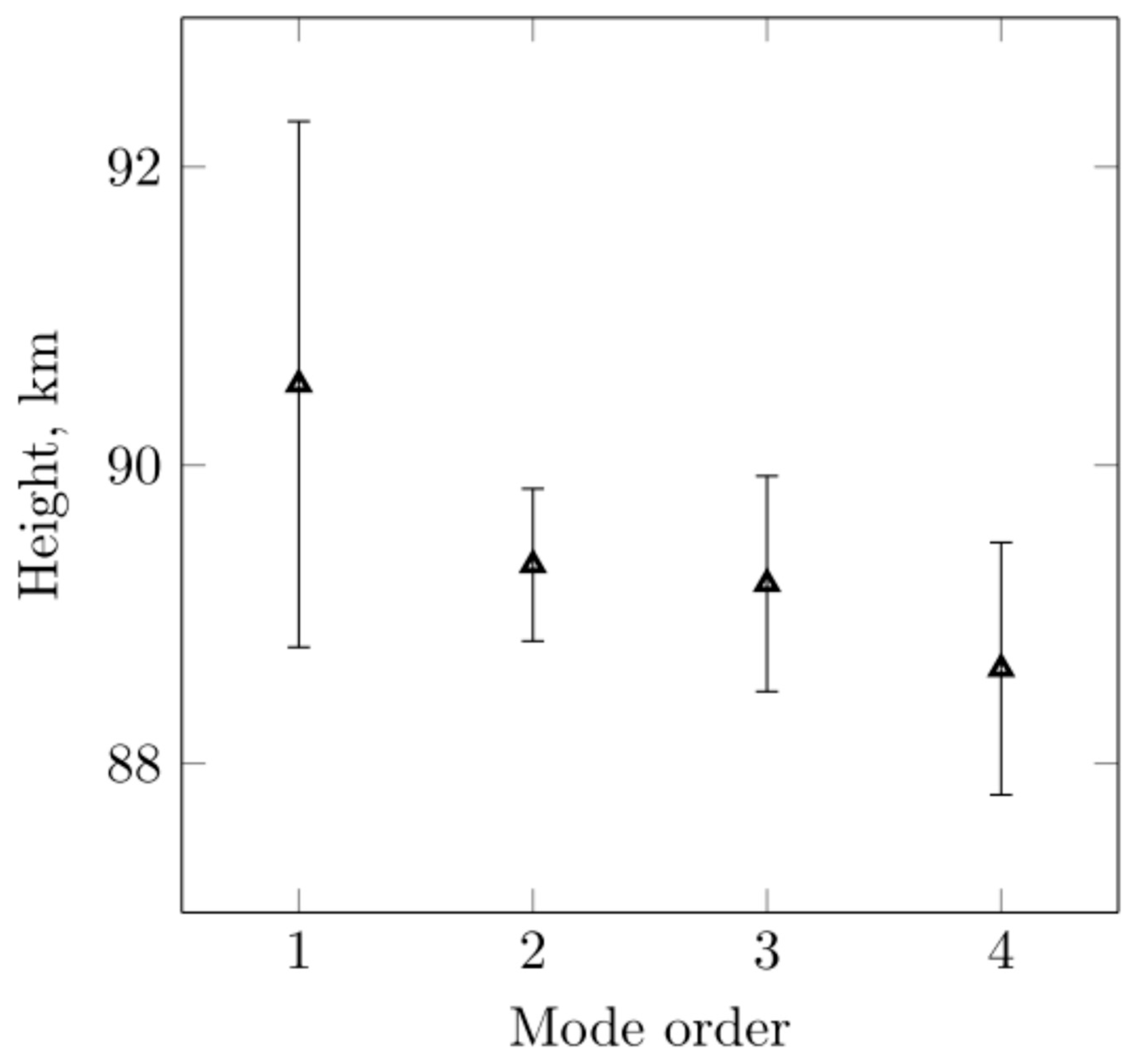
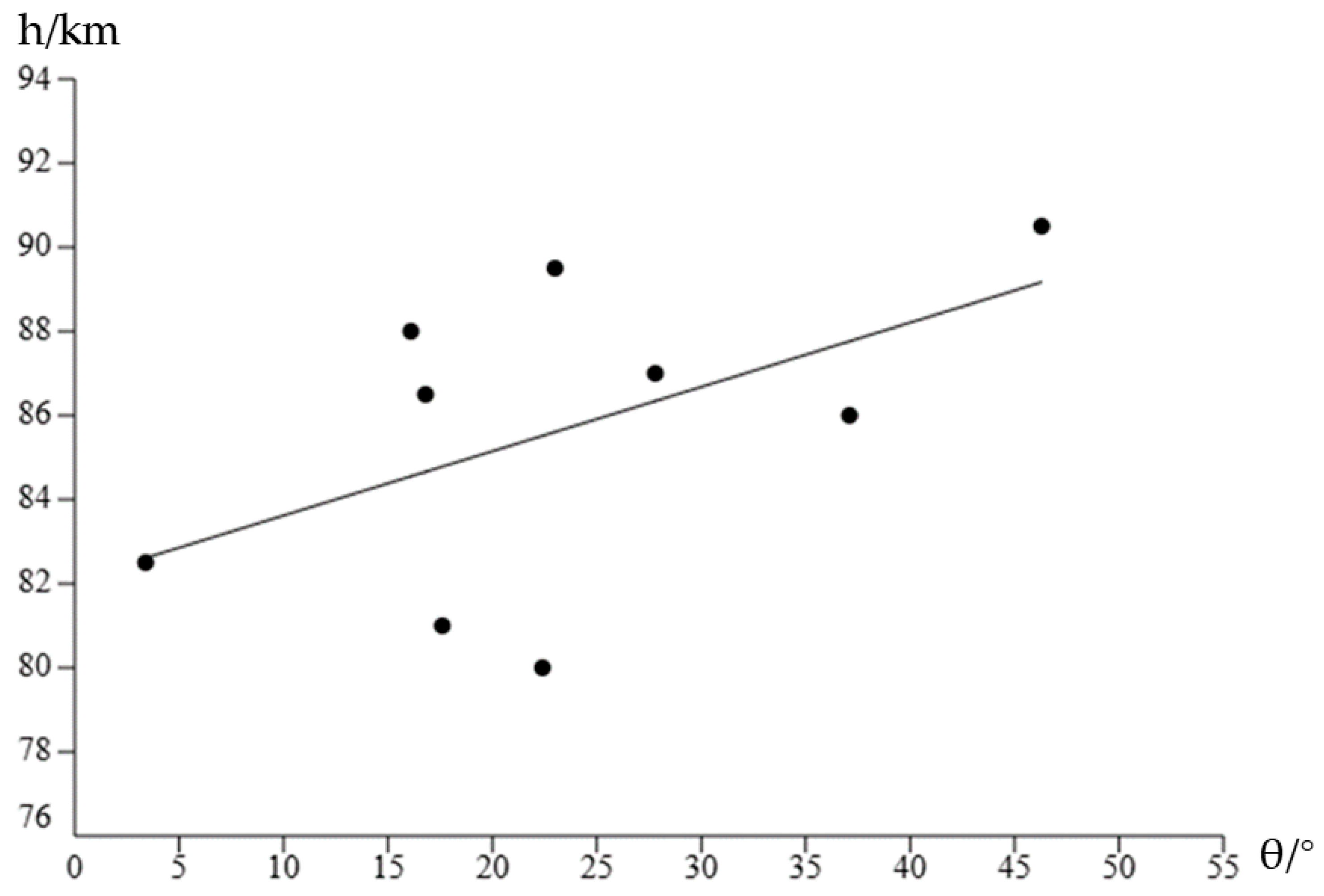
Shvets et al. [43] discussed tweeks recorded at Kharkov, Ukraine (geomagnetic latitude +46.3° [23]). Their figure, reproduced here as Figure 3, claims to show that the effective height of the waveguide is essentially constant, or decreases slightly, as the wave mode number increases from 1 to 4. They also showed that the waveguide height generally increases as the night progresses from 18 to 24 UT [43], as deduced from tweeks generated in four different thunderstorm centres that were from 500 to 1400 km from the receiving station.

Using recordings made at IZMIRAN in Moscow, Russian Federation (geomagnetic latitude +51.7° [23]), Reznikov et al. [44] presented the waveform of a night-time tweek, its instantaneous frequency, and its polarisation (mainly left-handed in the tweek’s “tail”, from 30 ms after the initial lightning discharge until its termination at 46 ms). They demonstrated that near the reflection level the electron-neutral collision frequency, ν_en, is << ω_B, and absorption is small. However, if the reflection level were to be at lower heights, ~60 km, where ν_en ≥ ω_B, waves of ~1.8 kHz would be damped so that tweeks would not be expected to occur.

The modus operandi and performance of an automated tweek detection system were presented by Zhou et al. [45] using data recorded at Suizhou station, China (geomagnetic latitude +22.4° [23]). For such data in February 2016, Yi et al. [46] showed that the identified low-latitude tweek events’ occurrence rate varies considerably, from 800 to 6000 tweeks per day, and exhibits a strong diurnal and local time dependence, with the peak occurring before local midnight. “Estimates of the propagation distance and ionospheric reflection height of tweek atmospherics suggest that the majority (~92%) originate from the lightning activity within a radius of 4000 km and that they are very likely to reflect from the lower ionospheric D-region at the height range of 75 to 85 km. At these lower ionospheric reflection altitudes, ~74% of the corresponding electron densities from the tweek spectral measurements are within the range from 24.5 to 27.5 × 10⁶ m⁻³ [46].

Zhang et al. [47] considered tweeks observed in China, near the border with Ladakh in India (geomagnetic latitude +27.8° [23]), between 2004 and 2012. Their automatic system picked out the dispersion curve of tweeks and gave N_eR1 between 27.6 and 31.0 × 10⁶ m⁻³ and h_R1 between 82 and 92 km, with the propagation distance ranging from 1300 to 3900 km; these values correspond to ± one standard deviation.

Another automated system was described by Maslej-Krešňáková et al. [22]. They developed a reliable automatic method for extracting the required details from the frequency–time spectrograms, based on a deep learning and deterministic approach. The method can detect sferics and tweeks from spectrograms and, in post-processing, determine to the nearest millisecond the time that the event occurred.

Ohya et al. [14] estimated nighttime electron densities in the D-region ionosphere at low to middle latitudes by accurately reading the first-order mode cut-off frequency of tweek atmospherics received simultaneously at Moshiri and Kagoshima in Japan. Equivalent electron densities ranged from 20 to 28 × 10⁶ m⁻³ at ionospheric reflection heights of 80 to 85 km. A comparison of their estimates with electron density profiles obtained from the IRI-95 model [25], medium frequency radar measurements, and rocket experiments revealed almost consistent results for the lower D-region. Ohya et al. [48] developed a method of estimating tweek reflection heights in the D-region from accurate measurements of their first-order mode cut-off frequencies (~1.8 kHz).

Ohya et al. [49] presented an automated procedure to use f_c1 values derived from tweeks observed at Kagoshima and their frequency-time dispersion relation to estimate the distances to the lightning sources. Their Figure 8 shows the variation of h_R1 from 11 to 21 December 2006, with a large magnetic storm occurring during local daytime on 15 December. In the storm recovery phase, h_R1 increased from 92 to 97 km over three hours. This indicates the production of D-region ionisation by charged particle precipitation from the magnetosphere at a rather low magnetic latitude during the main phase of the geomagnetic storm (see Section 6).

Ohya et al. [15] showed that the duration of rare daytime tweeks, with m = 1 or 2, was ~12 ms, shorter than for night-time ones (~50 ms) [14]. They concluded that the daytime tweeks propagate over shorter distances, with larger attenuation during their propagation in the waveguide. This could be due to the sunlit D-region ionosphere being lower during the day than at night. The best conditions for daytime tweek occurrence were found to be when the bottom side of the ionosphere is sharply defined and the ionosphere is rather high [15].

Table 1. Station names, their geomagnetic latitudes, ionospheric reflection heights and references to the papers presenting significant results on tweeks.

Station	Geomagnetic Latitude (°)	Reflection Height, hR1 (km)	References
Northern Finland	+64.8	-	[38]
IZMIRAN, Moscow, Russia	+51.7	-	[44]
Kharkov, Ukraine	+46.3	89–92	[43]
Tunisia	+37.1	77–95	[21]
China, near Ladakh, India	+27.8	82–92	[47]
Kagoshima, Japan	+23.0	86–93	[33]
Suizhou, China	+22.4	75–85	[45,46]
Lucknow, India	+17.6	81	[28,29]
Varanasi, India	+16.8	83–90	[30]
Allahabad, India	+16.1	86–90	[18,19]
Vietnam	+3.4	80–85	[31,32,33]
Malaysia	−6.7	73–87	[35]
Suva, Fiji	−22.1	84	[24,26]
Palmer, Antarctica	−55.7	65–82	[36]
Akademik Vernadsky, Antarctica	−56.2	87.3	[20,39]
Maitri, Antarctica	−67.7	64–79	[25]

summarises the results presented in this section.

Useful comparative information has been discussed by Thomson et al. [50]. Rocket measurements are summarised and supplemented with D-region production-loss modelling, giving rise to a near-global model named FIRI-2018 (Faraday International Reference Ionosphere, see Section 7). This provides electron number densities as functions of height, latitude (<60°), solar zenith angle, and F10.7 cm solar flux. These rocket-based electron density values are compared with the corresponding values derived from VLF measurements, by day at a low latitude (~20°) and a high mid-latitude (~55°), and by night mainly at mid-latitudes. The agreement is fairly good in the common height range ~60 to 75 km, with the changes with solar zenith angle being comparable. For daytime high mid-latitudes, the agreement is less satisfactory, particularly at the lowest common altitudes, with the VLF measurements showing the expected effects of the production of ionisation by cosmic rays much more than the rocket-based values do. The D-region description in the FIRI-2018 model is significantly better than the earlier IRI-2016 model [25].

Baumann et al. [51] studied the “D-region electron density during sunrise and sunset as observed by the incoherent scatter radar in Arecibo (Puerto Rico). The observations show significantly lower electron densities during morning hours compared to evening hours when considering solar zenith angles (SZAs) between 80° and 100°; for lower SZAs the electron densities do not differ significantly. This asymmetric behaviour is observed for altitudes between 90 and 75 km altitude”. The asymmetry originates from a higher electron–ion recombination rate than the ionisation rate during sunset [51]. They compared their results with the predictions of ion chemistry models of the D-region.

To summarise, the simplest interpretation of tweeks, whose duration is typically up to 40 ms, is that they identify the cut-off frequency of the Earth-ionosphere waveguide at ~1.8 kHz and that the electron density at the ionospheric reflection level of ~83 km is ~27 × 10⁶ m⁻³. The reflection level h_R1 lies between 80 and 90 km. It generally rises by up to ~5 km during the local night and in summer can be ~5 km higher than during the winter. However, other stations report that it is a few km lower in summer. It does not exhibit any consistent variation with geomagnetic activity. This reflection height displays a tendency to increase with increasing geomagnetic latitude, as might be expected from the decrease in the daytime solar zenith angle causing a higher ionosphere as latitude increases. Whilst tweeks are primarily a night-time phenomenon, they are observed through the sunrise and sunset periods and are occasionally seen during the daytime when their duration is only ~12 ms. Then the upper atmosphere is photo-ionised by the Sun’s extreme ultraviolet radiation and X-rays, with the electron production rate depending on the solar zenith angle. The D-region is lower by day than at night, and so the attenuation during propagation in the waveguide is then much greater. A more detailed interpretation by Shvets et al. [39] shows that the tweek spectrum depends on the interference between different modes propagating in the waveguide. This method gives an electron density that is two orders of magnitude larger at the reflection level and which rises by a few km during the night. It also makes possible a determination of the distances to the thunderstorms causing the tweeks.

3. Tweeks Observed During a Solar Eclipse

As already mentioned, Burton and Boardman [1] discovered and named tweeks. Their observations were made on 31 August 1931 in New Hampshire, USA, during a total solar eclipse. They noted that 17 tweeks occurred during the onset of the eclipse and until just after totality. Further, they found that the intensity of audio frequency radio signals showed an “abrupt rise shortly before the time of eclipse totality and an abrupt fall after totality. The duration of this period of high intensity is 55 min, its mid-time occurring 5 min after mid-totality”.

Rycroft and Reeve [52] and Reeve and Rycroft [53] recorded naturally occurring VLF radio signals in Newfoundland during the total solar eclipse of 7 March 1970. “Some of the atmospherics received were tweeks, normally characteristic of night-time propagation conditions, each of which has a sharp low-frequency cut-off which gives information on the height of the ionospheric reflector. This varies from 69 km at the start of the eclipse to 76 km at maximum totality and to 69 km at the end; these heights are somewhat less than those measured at totality by rocket methods, since the effects of the conical perturbation to the ionosphere are integrated over the propagation path from source to receiver” [53]. They used meteorological satellite photographs to identify the thunderstorm from which the lightning originated.

Kozlov et al. [54] reported a ~40% increase in the number of atmospherics received at Yakutsk, Russia, during the 29 March 2006 solar eclipse; most of these originated from central Africa. This result is in accord with [1].

For the 1 August 2008 solar eclipse investigated at Kolkata, India, De et al. [55] showed that the amplitudes of sferics at 1, 3, and 5 kHz were about 60% greater during the period of near totality than at similar times on other days nearby. On the other hand, De et al. [56] noted a decrease in the amplitude of sferics at 81 kHz observed at Tripura University, Agartala, in India, during the 22 July 2009 eclipse.

Singh et al. [57] discussed observations of tweeks with m > 1 at the low-latitude stations Allahabad and Nainital, India, during the total solar eclipse of 22 July 2009. At Allahabad the eclipse was total, and at Nainital 85%. With about 30 to 40% obscuration of the solar disc, tweeks can occur. A total of 148 tweeks at Allahabad and 20 tweeks at Nainital were recorded, with some up to m = 3. The World Wide Lightning Location Network (WWLLN) data indicated that the tweeks were generated by lightning in the partially eclipsed Asia-Oceania region. Changes in the D-region ionospheric VLF reflection height and in the electron density at the reflection level (22 to 23 × 10⁶ m⁻³) during the eclipse were estimated from f_c1. Two figures were presented [57], showing that the reflection height increased from ~89 km for the first tweek to about 91 to 92 km at totality and then decreased to ∼87 km at the end of the eclipse. These reflection heights are some 2 to 3 km lower than normal night-time tweek reflection heights. This indicates that a partial night-time condition is created during the eclipse, as the main D-region ionising radiation, Lyman α, is blocked, but solar soft X-ray and extreme ultraviolet radiations originating from the solar corona just above the limb are not totally blocked and so produce some ionisation in the D-region.

Ohya et al. [58] reported observations of daytime tweeks, with durations of only 6 to 21 ms, during the solar eclipse of 22 July 2009 at Moshiri and Kagoshima, Japan, where the percentages of the eclipse totality were 46% and 97%, respectively. The average m = 1 reflection height, h_R1, was 95 km at Moshiri, almost the same as that for normal nighttime conditions, and 87 km at Kagoshima. The tweek reflection heights there ranged from 80 km to over 100 km, suggesting a large difference of electron densities in the lower ionosphere between totally and partially eclipsed regions. Ohya et al. [58] also observed the phase variation of LF transmitter signals during the eclipse. The average change in the phase delay of the LF signals due to the lengthening propagation distance was 109° for signals propagating across the eclipse path and 27° for those that did not. Assuming a normal daytime reflection height for LF waves of 65 km, a ray tracing analysis indicated that the variations in phase corresponded to a height increase of 5 to 6 km for the propagation across the eclipse path and 1 to 2 km for partial eclipse conditions.

For the total solar eclipse over in Europe on 11 August 1999, Clilverd et al. [59] reviewed measurements made of the amplitude and phase of four VLF transmitter signals in the frequency range of 16 to 24 kHz. Significant variations in phase and amplitude were reported for 17 paths to 5 stations, with distances from transmitter to receiver ranging from 90 km to 14.5 Mm, with most being <2 Mm. Typically, positive amplitude changes were observed throughout the whole eclipse period on path lengths < 2 Mm, while negative amplitude changes were observed on paths > 10 Mm. Negative phase changes were observed on most paths, independent of path length. Although there was significant variation from path to path, the typical changes observed were ~3 dB and ~50°. The changes observed were quite accurately modelled using the Long Wave Propagation Capability (LWPC) waveguide code [60]. The ionosphere became higher and sharper as totality approached. Using a D-region chemistry model, the calculated electron concentration values at 77 km altitude throughout the period of the solar eclipse showed good agreement with the values determined from observations at all times, which suggests that a linear variation in the electron production rate with solar ionising radiation is reasonable.

Guha et al. [61] investigated changes in equatorial D-region electron densities using sub-ionospherically propagating VLF signals at 18.2 kHz received at Tripura University, over a distance of 2.2 Mm during the total solar eclipse of 22 July 2009. The results show an average decrease of 3.2 dB in signal strength, compared to control days, during the peak solar obscuration over the propagation path. During the maximum eclipse period over the path, the model profile showed an average 80% decrease in the electron density at a height of 71 km in the equatorial lower ionosphere. Cohen et al. [62] presented results on VLF and LF radio propagation under the ionosphere when the total solar eclipse over the USA on 21 August 2017 was happening; however, they did not comment on naturally occurring radio signals. They found a gradual rise and fall of signal strengths on almost all paths as the eclipse advanced and then declined, as VLF signal attenuation is reduced and then increased by the changing ionosphere under the eclipsed Sun [62].

Ohya et al. [63] noted that the “occurrence number of tweeks increased during the solar eclipse, which shows that electron density decreased and the reflection coefficient in the lower ionosphere increased”. Further, they found that during the solar eclipse that occurred from 01.34 to 06:59 UT on 20 April 2023, a “variation in VLF amplitude of about 2 dB was observed for the NWC-KAG (North West Cape, Australia—Kagoshima, Japan) path, which was less than that at sunset/sunrise time. The reflection height at the mid-point of the NWC-KAG path increased by 8 km compared with usual daytime”.

Table 2. Summary of solar eclipse effects on VLF/LF radio transmitter signals and tweeks.

Date of Eclipse	Station	Effects	References
31 August 1932	Conway, New Hampshire, USA	17 tweeks recorded, most near eclipse onset	[1]
7 March 1970	Newfoundland, Canada	hR1 increased from 69 km to 76 km at totality, ~6 dB increase in intensity of static at totality	[52,53]
11 August 1999	Europe	50° phase changes of VLF transmitter signals are interpreted as raising and sharpening of D-region	[59]
29 March 2006	Yakutsk, Russia	40% increase in number of sferics	[54]
1 August 2008	Tashkent, Uzbekistan	hR1 raised from 84 km to 91 km	[64]
1 August 2008	Kolkata, India	60% increase in amplitudes of sferics at a few kHz	[55]
22 July 2009	Tripura, India	Decrease in amplitudes of sferics at 81 kHz	[56]
22 July 2009	Allahabad, India	Changes in tweek reflection heights during eclipse	[57]
22 July 2009	Agartala, India	VLF transmitter signal phase change interpreted as 80% electron density at 71 km altitude	[61]
22 July 2009	Kagoshima, Japan	hR1 = 87 km at totality	[58]
22 July 2009	Kagoshima, Japan	LF signal phase change interpreted as 6 km rise of ionospheric reflector	[58]
21 August 2017	USA	VLF/LF radio signal amplitude and phase changes	[37,62]
20 April 2023	South East Asia and Australia	More tweeks during eclipse than normal daytime	[63]
20 April 2023	South East Asia and Australia	Reflection height of NWC (19.8 kHz) to Kagoshima, propagation path raised by 8 km	[63]

summarises the results presented in this section.

Lay et al. [65] and Smith et al. [66] have recently used broadband lightning waveforms from the Earth Networks Total Lightning Network (ENTLN) to probe the D-region ionosphere (60 to 90 km altitude). Each waveform contains a ground wave and a time-delayed ionospheric reflection. The time delay between the ground wave and ionospheric reflection has previously been used to estimate a single specular reflection altitude where LF/VLF waves are reflected by the ionosphere [65]. The diurnal D-region height variation and time variations on the order of tens of minutes to hours were evident in the measurements [63]. The diurnal variations were compared with those obtained using a D-region model from the IRI [25].

Summarising, the occurrence of tweeks was first noted during a solar eclipse [1]. The tweeks have durations up to ~20 ms: their reflection level rises by ~7 km as totality approaches and then falls. Valuable complementary information on the lower ionosphere is obtained by monitoring VLF and LF transmitter signal amplitudes and phases under eclipse conditions and interpreting them using waveguide theory.

4. Sferics and Volcanoes

Mather and Harrison [67] have reviewed different conceptual theories for charge generation and separation in volcanic plumes that have been developed to explain the disparate observations obtained. It is unclear which mechanisms or combinations of electrification mechanisms dominate in different circumstances. Electrostatic forces play an important role in modulating the dry fall-out of ash from a volcanic plume. Beyond the local electrification of plumes, the higher stratospheric particle concentrations following a large explosive eruption may affect the global atmospheric electrical circuit. Rycroft et al. [68] have recently used observations of volcanic lightning to determine that the time constant of the global electric circuit (GEC) [69] is ~10 min.

Cimarelli and Genareau [70] have reviewed the electrification of volcanic ash plumes and the occurrence of volcanic lightning, detailing the most recent findings concerning electrification mechanisms of eruption columns/plumes (tribo-electrification, fracto-electrification) and how hydrometeor charging contributes to this electrification depending upon the eruption style and abundance of water. Field measurements to determine the charge structure of volcanic ash and gas plumes revealed a wide variability, both spatially and temporally, indicating the influence of these different charging mechanisms.

Larnier et al. [71] introduced a new methodology to automatically detect and characterise radio waves from lightning using a time–frequency decomposition obtained through the application of a continuous Morlet wavelet transform. They concentrated on three sources, namely, atmospherics, slow tails, and whistlers, that cover the frequency range from 10 Hz to 10 kHz; each wave has distinguishable characteristics in the time–frequency domain due to the source and to dispersion processes. They then applied the method to real audio-magnetotelluric data acquired at three stations on Guadeloupe, French Overseas Departments and Territories. One receiver was located 0.6 km from the Soufriere Volcano Observatory. Most of the analysed atmospherics and slow tails (0.1 to 1 kHz) displayed linear polarisation, whereas the whistlers were elliptically polarised, as expected. They showed a reduction in the power spectrum from 1.7 to 1.8 kHz, which can be attributed to the m = 1 cut-off frequency. No signals associated with nearby volcanic activity were reported.

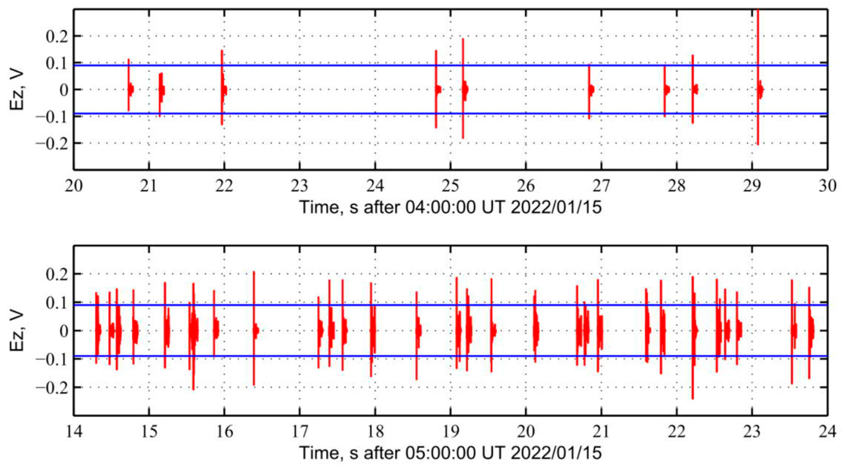
Figure 4 displays strong tweek waveforms over a period of 10 s generated by volcanic lightning [72]. Shvets et al. [72] reported an order of magnitude increase in the VLF and ELF radio noise power and in the number of VLF atmospherics, including slow tails, observed during the explosive eruption of the Hunga Tonga-Hunga Ha’apai (HT-HH) volcano, on 15 January 2022, at the Akademik Vernadsky station in Antarctica, ~8870 km from the volcano. At the peak of activity, around 5 UT, the number of atmospherics received in a 2 min interval was almost 15 times more than in the period before the eruption. Their measured bearing was from 242° to 243° from North. There were ~360 VLF atmospherics per second, whereas the annual average lightning flash rate is 44 ± 5 s⁻¹ (intra-cloud and cloud-to-ground lightning combined) [73]. According to the WWLLN [74], the increased thunderstorm activity was concentrated very close to the volcano during this period. The discrepancy between the observed intensities of ELF (~0.1 to 1 kHz) and VLF (~3 to 15 kHz) radiation suggests a significant difference between the currents in the lightning discharges occurring near the volcano vent and those in the volcanic ash plume [67,72].

Bor et al. [75] have discussed the responses of the AC and DC global electric circuits to the large eruption of the HT-HH volcano, which occurred on 15 January 2022. According to data from the GLD360 and WWLLN (VLF) lightning detection networks, the peak lightning stroke rate, 83 s⁻¹, was dominated by negative polarity lightning, but the distributions of positive and negative lightning discharges in latitude and longitude around the volcano differed. A global intensification of Schumann resonance (SR) signals between ~5 and 40 Hz [11,44,69] occurred in connection with the enhanced lightning activity caused by the eruption. SR data-based results confirm that the lightning activity in the eruption dominated the naturally occurring global activity for a period of about an hour. The highly localised increase in lightning activity over the volcano was a unique point source of SR excitation [75]. Because this event happened during the local afternoon, tweeks were not investigated in their study [75].

Ohya et al. [63] considered that the explosive eruption of the submarine volcano HT-HH provided the opportunity to study interactions between the atmosphere and ionosphere caused by Lamb and Pekeris waves [76]. Although Pekeris wave resonance had not been previously detected in the D-region ionosphere, their study [63] using multi-point monitoring of the lower ionosphere (with the Asian VLF Observation Network, AVON) and of the atmospheric electric field did so. They observed that “oscillations of 100 to 200 s were observed in LF transmitter signals and magnetic and atmospheric electric fields due to Pekeris waves, although no corresponding atmospheric pressure changes were detected on the ground. Simulations showed Pekeris waves oscillating near the mesopause, suggesting resonance, which projected onto the Earth’s surface through a global electric circuit” [77].

In summary, HT-HH volcanic lightning generating VLF radio signals happened during the local afternoon in summer, and so no tweeks occurred. The rates at which volcanic lightning discharges were produced were up to an order of magnitude larger than those of thunderstorm-generated lightning. The intensity of SR increased markedly during the Tonga eruption of January 2022. The explosive eruption of this volcano caused atmospheric oscillations with periods ~100 to 200 s, which were detected using VLF radio observations.

5. Ionospheric Changes and Tweeks Observed Before Large Earthquakes

In the early years of the 21st century, the rapid development of Global Navigation Satellite System (GNSS) techniques made possible the realistic mapping of the total electron content (TEC) of the Earth’s ionosphere on a global scale [78,79]. Here TEC is the total number of electrons in a vertical column of 1 m² cross section from below the D-region, up through the E- and F-regions and into the topside ionosphere, up to the altitude of the GPS satellite. One TEC unit (TECU) contains 10¹⁶ electrons m⁻².

Le et al. [80] used the TEC data from the global ionosphere map for a total of 736 M ≥ 6.0 earthquakes around the globe from 2002 to 2010. Their results showed that the occurrence rate of an anomaly several days before these large earthquakes is greater than that on other days, especially for the large magnitude and low depth earthquakes. These results [80] indicated that the anomalous TEC behaviour just a few days before the earthquakes is related to the forthcoming earthquakes with a high probability. However, Ikuta and Oba [81] conducted the same analysis using a random sequence of synthetic earthquakes, finding that the anomalous day rate that is comparable to their result occurs in ∼40% of the thousand random trials, suggesting that their result [80] may be an artifact. Thus, it is important to investigate the authenticity of claims such as those made by Le et al. [80].

Liu et al. [82] studied pre-earthquake ionospheric anomalies (PEIAs) using ionospheric plasma observations made aboard a satellite and global maps of the TEC for the M = 7.3 earthquake in the Iran–Iraq border region on 12 November 2017, as well as the signatures of two magnetic storms on 7 and 21 to 22 November 2017. Anomalous increases of both the TEC and ionospheric ion density over the epicentre area on 3 to 4 November, about 8 days before this large earthquake, agreed with the temporal PEIA characteristics that such a statistically significant TEC increase frequently appears 6 to 14 days before 53 M ≥ 5.5 earthquakes in the area from 1999 to 2016.

Feng et al. [83] proposed a new method for detecting TEC anomalies before an earthquake, taking the M = 7.8 earthquake in Türkiye on 6 February 2023 as an example. They analysed the Centre for Orbit Determination in Europe, Global Ionospheric Map (CODE GIM) data from a global perspective, and showed that the ionospheric TEC anomalies on 20 and 27 January and 4 and 5 February 2023 may be precursors of the earthquake. However, Akhoondzadeh [84] used five classical and intelligent anomaly detection algorithms to detect seismic anomalies in the time series of TEC changes from 1 November 2022 to 17 February 2023. All these algorithms showed outstanding anomalies in the 10 days before the earthquake, with one method showing clear TEC anomalies 1, 2, and 3 days before the event. With the second method, pre-seismic anomalies were observed 1, 2, 3, 5 and 10 days prior to the main shock. The third method emphasised the abnormal behaviour of the TEC parameter 1, 2, 3, 6, and 10 days before the earthquake [84]. It is concluded that the identification of a reliable precursor some days before a large earthquake is not a straightforward matter.

Ma et al. [85] presented a statistical study of pre-earthquake vertical total electron content (VTEC) variations for 1522 shallow (≤60 km) strong (M ≥ 6.0) earthquakes around the world from 2000, classified according to different magnitudes, latitudes, and focal depths. The results showed a significant correlation between the probability of anomalies occurring (Po) and epicentral latitudinal locations from 1 to 10 days before earthquakes, especially for larger earthquakes in the equatorial and low-latitude regions.

A study to investigate pre-earthquake anomalies using both geomagnetic field and TEC variations for the 60 days preceding and 5 days following 694 earthquakes with magnitudes ≥ 5 in 2011 in and around Japan was carried out by Zulhamidi et al. [86]. Days with geomagnetic storms were excluded from the analysis. Both geomagnetic and TEC precursors were significantly found for moderate and shallow earthquakes. Geomagnetic precursors occurred at the higher rate of 65% than did TEC precursors (11%), although in 3% of the cases, both types were detected. Such anomalies occurred up to 30 days before the earthquake [86].

Ullah et al. [87] recently investigated seismo-ionospheric and atmospheric anomalies associated with two offshore Japanese earthquakes with magnitudes > 7. Anomalies were identified using three statistical techniques: (a) mean ± standard deviation, (b) median ± interquartile range, and (c) wavelet transform-based detection. All methods revealed anomalies 4 to 10 days before and 3 to 5 days after the events. The median method demonstrated robustness against outliers, identifying stable anomalies, such as a 19% TEC deviation detected three days prior to the Mw 7.3 earthquake, which occurred under geomagnetically calm conditions.

Using regional GPS networks, He and Heki [88] studied the three-dimensional spatial structure of ionospheric TEC anomalies preceding three large (M > 8) earthquakes in Chile, South America, in 2010, 2014, and 2015. Both positive and negative TEC anomalies appeared simultaneously 20 to 40 min before the earthquakes. For the two midlatitude earthquakes (2010 and 2015), positive anomalies occurred to the north of the epicentres at altitudes of 150 to 250 km. The negative anomalies occurred farther to the north at higher altitudes, 200 to 500 km. This means that the epicentre and the positive and negative anomalies are all aligned parallel to the local geomagnetic field, which is the typical structure of an ionospheric anomaly occurring in response to positive electric charges on the Earth’s surface. However, such a feature could be due to a decrease in the background TEC after the earthquake, rather than an enhancement before it [89]. “It thus appears likely that the reported TEC enhancements are artifacts” [89].

Zhu et al. [90] used TEC data from the Internet GPS Service (IGS) and examined 50 earthquakes of magnitude Ms ≥ 7.0 worldwide between 2007 and 2009. They found significant anomalous increases and decreases about 7 days prior to 94% of the earthquakes, mostly between 12 and 18 LT.

Torjiev et al. [64] established a VLF recorder at Tashkent, Uzbekistan (geomagnetic latitude +33.8° [23]); they also found anomalous TEC values before and during the M = 4.4 earthquake there on 4 August 2008. They also made observations during the 1 August 2008 solar eclipse (see Table 2).

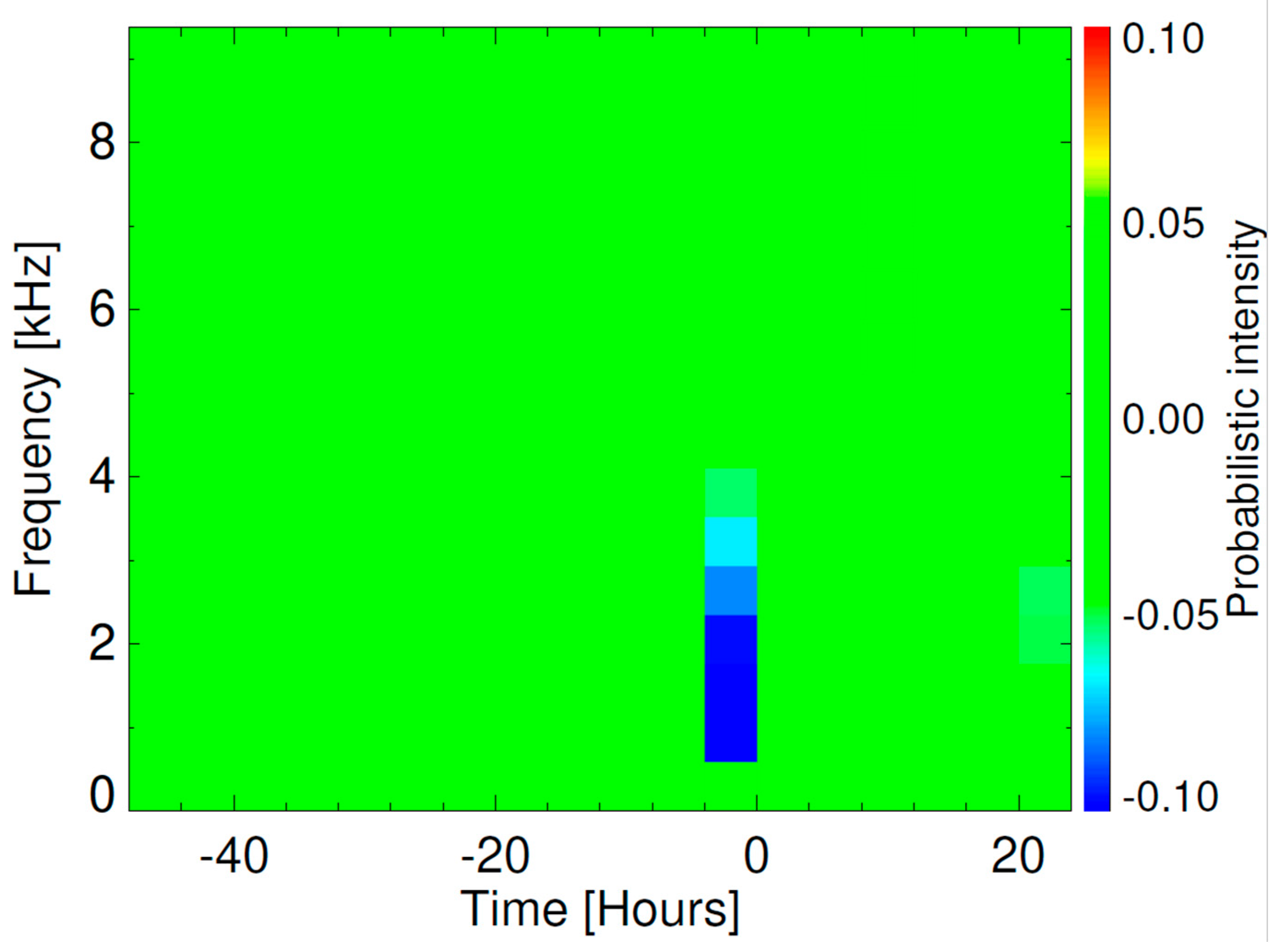
Nemec et al. [91] presented the results of a statistical study of the intensity of VLF electromagnetic waves observed in the vicinity of earthquakes. A unique set of data obtained aboard the French micro-satellite DEMETER (at an altitude of about 700 km, in a nearly Sun-synchronous polar orbit) and a robust data processing procedure were used. The changes of wave intensity in ~15 bands (with ~120 Hz bandwidth, to avoid interference) at frequencies up to 10 kHz due to seismic activity were investigated and their statistical significance evaluated. More than 2.5 years of satellite data were analysed and about 9000 earthquakes with magnitudes ≥ 4.8 that occurred all over the world were included. With data from 50 orbits, their Figure 2 (right) shows that, during the night, there was a statistically significant (by 4 standard deviations) decrease, of 4 to 6 dB, of the measured ~1.0 to 2.4 kHz wave electric intensity, shortly (from 0 to 4 h) before an intense surface earthquake. Their Figure 3 shows that such an earthquake (M > 5, depth ≤ 40 km) occurred within a horizontal distance ~350 km of the satellite’s footprint on the Earth’s surface. This result provides a very clear association between a reduction (by 4 to 6 dB) of the 1 to 2.4 kHz natural signal intensity within the preparation zone of a large earthquake some hours before the earthquake struck. The authors concluded that “the frequency band where the decrease is observed could be related to the cut-off frequency of the first transverse magnetic (TM) mode in the Earth-ionosphere guide (1.7 kHz during the night-time). Finally, our analysis shows that the effect is connected only with surface earthquakes” [5,91].

Nemec et al. [92] focussed on the detailed analysis of the decrease in wave intensity shortly before the main shock that was observed during the nighttime. Using a larger set of data (more than 3.5 years) and a newly developed data processing method, they confirmed the existence of a very small but statistically significant decrease in wave intensity up to 4 h before the time of the main shock at frequencies of about 1.7 kHz. The decrease does not occur directly above the earthquake epicentre but is shifted about 200 km westward. Moreover, it more often occurs close to shallower earthquakes and close to earthquakes with larger magnitudes.

Using a much larger set of DEMETER (Detection of Electro-Magnetic Emissions Transmitted from Earthquake Regions) observations, Pisa et al. [93] first calculated the expected unperturbed distribution of the power spectral densities of electromagnetic emissions. The power spectral densities measured above the vicinities of earthquakes were then compared with the unperturbed distribution and examined for the presence of uncommon effects related to seismic activity. The statistical significance of the observed effects confirmed the previously reported results [91] of a very small, but statistically significant, decrease in wave intensities a few hours before the times of the main shocks. This effect is very small (a decrease of ~2 dB) as compared to the usual variations in the background activity (±7.5 dB), and therefore it is very difficult to observe it directly in specific cases. The decrease in wave intensity at a frequency of ~1.7 kHz, observed only during the night and only for shallow earthquakes, could be explained by increases in the cut-off frequency of the Earth-ionosphere waveguide due to the production of extra ionisation at the bottom of the D-region caused by imminent earthquakes.

In his PhD thesis, Pisa [94] studied plasma density variations in the vicinity of the very powerful earthquake in Chile (Mw 8.8), which occurred on 27 February 2010. Data recorded before the main shock along orbits close to the forthcoming epicentre showed a large plasma density increase. A statistical analysis using four years of data to monitor plasma density variations under similar conditions showed that a large increase in the plasma density was very uncommon at this location and season—thus, this could be an earthquake precursor. Further, a statistical study (over ~6.5 years of the mission) of variations of VLF wave intensity for all available data measured close (in time and distance) to large earthquakes (M ≥ 5) confirmed the previously reported results [91,92] of a statistically significant decrease in the wave intensity at frequencies of about 1.7 kHz.

Pisa et al. [95] checked for the presence of statistically significant changes of natural VLF wave intensity related to pre-seismic activity using all the relevant data acquired by DEMETER. They compared data from the vicinity of about 8400 earthquakes with an unperturbed background distribution to evaluate the statistical significance of the observed effects. This confirmed the presence of a small, but statistically significant at the 95% level (2.3 standard deviations), decrease in the wave intensity (by ~2 dB) at frequencies of about 1.7 kHz. “Altogether, more than 2000 spectra from 58 earthquakes (M ≥ 5) were used” [95]. The effect was observed for a few hours before the times of the main shocks, when the distance of the satellite’s footprint on the surface was within ~440 km of the forthcoming earthquake, and at night. “The effect is stronger for shallow earthquakes than for deeper ones”, <33 km [95]. The effect was found to be stronger between March and August (when global lightning activity is greater), at higher geomagnetic latitudes (>20°) and for earthquake foci below the sea. An important figure from their paper [95] showing a significant reduction of ~1 to 3 kHz signal intensity in the four hours before a large earthquake is reproduced here as Figure 5. The explanation could be that the D-region boundary of the ionosphere is lowered by ~2 km, and the waveguide becomes more attenuating, which leads to a decrease in the intensity of up-going fractional hop whistlers observed at the spacecraft [95]. This effect might result from a lowering of the ionosphere associated with an increase in the electrical conductivity of the lower troposphere due to an additional ionisation source of air molecules at the Earth’s surface prior to earthquakes. The existence of the effect for earthquakes under the sea rather than on land could be explained by the smaller attenuation of VLF waves propagating in the Earth-ionosphere waveguide over the good conducting sea and not over the poorly conducting land surface.

Zahlava et al. [96] have discussed up-going whistlers observed by DEMETER, which show some features of m = 1 and 2 tweeks; they are observed some 3000 km to the west of the thunderstorms that generated them. Toledo-Redondo et al. [97] used VLF electric field data recorded by DEMETER to monitor the first cut-off frequency (f_c1) of the Earth-ionosphere waveguide and to derive h_R1 values. 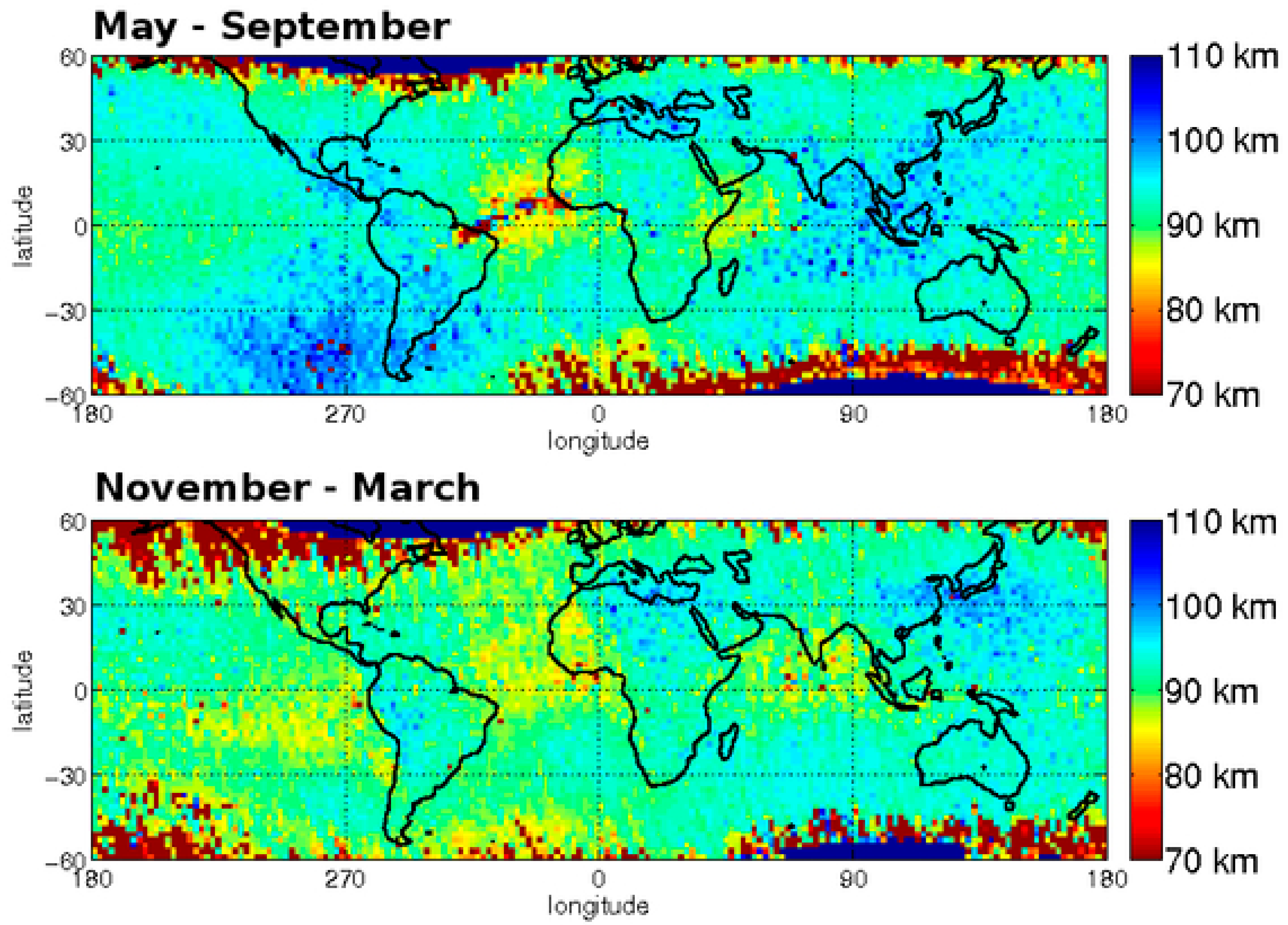From their paper [97], Figure 6 shows that this mode 1 reflection height is lowest within ±15° of the geomagnetic equator and at sub-auroral latitudes (L ~3). Table 1 here shows some tendency for the existence of such a pattern. It was also found [97] that the ionosphere was lower during the night over the oceans in the northern cold season. Parrot et al. [98] showed up-going fractional hop whistlers with the m = 1 cut-off frequency close to 1.7 kHz, and other mode cut-offs up to m = 5. At the time of these observations, the satellite was located a few thousand km west of the major southeast Asian thunderstorm centre.

Parrot et al. [99] explored multi-instrument space-borne observations in order to validate some physical concepts of Lithosphere–Atmosphere–Ionosphere Coupling (LAIC) in relation to four major destructive earthquakes, namely M8.6 on 28 March 2005 and M8.5 on 12 September 2007 in Sumatra, M7.2 on 21 March 2008 in the Xinjiang-Xizang border region, China (the Yutian earthquake), and M7.9 on 12 May 2008 in Wenchuan, China. The investigations concerned the ionospheric plasma density, Global Ionospheric Maps (GIMs) of the TEC, Thermal InfraRed (TIR) anomalies on the Earth’s surface, and Outgoing Longwave Radiation (OLR) from the Earth and its atmosphere and clouds. It is shown that all these anomalies could be identified as short-term precursors of the earthquakes, which can be explained by the LAIC concept proposed in [100].

An alternative mechanism for the coupling of processes at the Earth’s surface before large earthquakes via the atmosphere to the ionosphere has been suggested by Harrison et al. [101,102]. Termed Atmospheric Lithosphere–Ionosphere Charge Exchange (ALICE), their mechanism uses the increased electrical conductivity of the surface layer of air due to enhanced radon emission from the ground before a major earthquake to reduce the electrical resistance of the air column between the Earth and the ionosphere. This increases the downward fair-weather current in the GEC and, in order to maintain continuity of electron flow, lowers the ionosphere. This mechanism was already mentioned in relation to [95]. They suggested some experiments to be carried out some hours before a large earthquake to investigate this mechanism by measuring the cut-off frequency of tweeks, or the amplitude and phase of VLF radio waves propagating in the Earth-ionosphere waveguide, or medium frequency radar, incoherent scatter, or rocket studies of the D-region electron density profile. Not many such experimental studies have yet been realised. It is just possible that the effect on tweeks could be observed before a large earthquake in and around Europe by the UK Met Office lightning detection system named LEELA [103]. However, because of the ±7.5 dB variations in the background intensity of lightning-generated ~1.7 kHz noise, “it will therefore be very difficult to observe it directly in individual cases” [95].

Picozza et al. [104] have reviewed DEMETER and the Chinese/Italian (CSES-01) satellite observations of pre-seismic phenomena. They pointed out that the variety of phenomena associated with earthquakes requires the simultaneous observation of many parameters in space and below the ionosphere. The need for statistical studies that increase the reliability of results by reducing background effects requires more seismic events to be analysed worldwide. The CSES-02 satellite was launched on 14 June 2025; new results in this field are eagerly awaited.

Conti et al. [105] have given an overview of the observations carried out on the ground in order to identify earthquake precursors by distinguishing them from the background constituted by both natural non-seismic and artificial sources. They discussed measurements of mechanical parameters of the lithosphere, changes of groundwater and radon and other gas emanations detected before earthquakes, acoustic gravity waves in the atmosphere, and electromagnetic and ionospheric parameters. They focussed on some case studies and statistical analyses, together with the main hypotheses and models proposed in the literature to explain the observed phenomena, in a comprehensive study [105].

Yan et al. [106] studied the ionospheric ion densities at DEMETER over six years that were close, in both space and in time, to the epicentres of earthquakes and compared them with background values recorded at the same locations and under similar conditions. It was shown that, during the night, anomalous ionospheric perturbations related to earthquakes with magnitudes > 5 occurred up to 200 km from the epicentres and mainly five days before the earthquakes. Ion density perturbations also occurred just after the earthquakes and near the epicentres.

Nighttime electron densities and electron temperatures aboard CSES-01, in a Sun-synchronous circular orbit at 507 km altitude, were reported by Zhu et al. [107] above seismically active areas. For M > 5 earthquakes, positive electron density and negative temperature anomalies related to earthquakes mainly occurred ~1 to 7 days and ~13 to 15 days before the earthquakes, respectively, and within 200 km of the epicentres. For Ms ≥ 6.8 earthquakes that occurred globally between August 2018 and March 2023, Han et al. [108] found that electron density anomalies on the east side of the epicentre were significantly larger than those on the west side, and that the anomalies in the Northern hemisphere were mostly distributed south of the epicentre, whereas those in the Southern hemisphere were mostly north of the epicentre (as would be expected for the Earth’s dipolar magnetic field). The anomalies were more frequent on the day of the earthquake (a likely co-seismic effect) and 2, 7 and 11 days before the earthquake (precursors). For Ms ≥ 6.0 earthquakes in China, anomalous electron density values mainly occurred southwest of the epicentre [108], with the highest frequency observed 5 days before the earthquake, and there were continuous anomalous phenomena between 9 and 5 days before the earthquake. Li et al. [109] noted strong plasma density anomalies the day after the Wushi Ms 7.1 earthquake on 23 January 2024.

Li et al. [110] used more than three years of electron density data aboard the Swarm-B satellite, in an almost circular polar orbit at ~500 km altitude, to search for perturbations of ~150 to 2000 km spatial scale; a total of nearly 200,000 perturbations was found globally. Geomagnetic storms can enhance the plasma variations by more than 100%. Having eliminated those and perturbations at high latitudes, >±65°, more than 54,000 perturbations were kept to correlate with 3577 M ≥ 5.0 earthquakes worldwide within 15 days and 1500 km. The statistical results show that the seismo-ionospheric changes mainly occur five days before the earthquakes; they are not directly above them but up to 700 km away. This is interpreted as showing that the seismic influence propagates through the topside ionosphere along geomagnetic field lines.

To sum up the results presented in this section so far is difficult because they are so varied and somewhat contradictory between each other; the statistical significance of the results is often debatable. However, there are indications that, some hours, days, or weeks before a large earthquake, there can be real changes in the D-region ionosphere and in the TEC of the ionosphere. However, only two out of ten papers reported TEC anomalies one or two days before a large earthquake. Some mechanisms to account for these changes have already been alluded to.

Molchanov et al. [111] considered mechanisms to explain pre-seismic phenomena in the atmosphere and ionosphere. They showed that the upward migration of fluid substrate matter (bubbles) can lead to the expulsion of hot water/gas from the ground surface and cause an earthquake in the area whose strength has been weakened. Perturbations of the atmospheric density and temperature follow and could result in the generation of atmospheric gravity waves (AGWs, whose spectrum is discussed from a theoretical viewpoint in [112]), with periods ranging from 6 to 60 min. Such seismo-induced AGWs could lead to the modification of the ionosphere and changes to the conditions for radio wave propagation in the atmosphere.

The monograph of Sorokin et al. [113] comprehensively reviews models of the influence of earthquake preparation processes on the state of the near-ground atmosphere and the ionosphere through the electric field and currents occurring in the GEC. An extensive comparison of results of satellite-borne and ground-based observations of electric fields, plasma parameters, and electromagnetic waves before an earthquake is made as a validation criterion of the models. It is shown that the most complete explanation of precursor phenomena excited in the ionosphere and atmosphere and their interconnection can be provided by an electrodynamic model based on DC electric field generation due to the injection of charged aerosols into the atmosphere [114].

Hayakawa et al. [115] considered the additional current source in the GEC associated with the upward convective transport and the gravitational sedimentation of radon and charged aerosols injected into the atmosphere by soil gases. The enhanced DC electric field can reach the breakdown value at altitudes of 2 to 6 km, suggesting the creation of a peculiar seismic-related thundercloud that generates lightning whose VHF and VLF radiation could be studied.

Zhao et al. [116] have constructed an alternative LAIC model involving ELF electromagnetic waves of ~300 Hz radiated by earthquakes. The simulated EM field calculated at the altitude of the China Seismo-Electromagnetic Satellite (CSES-01) is compared with the sensitivity of electromagnetic sensors onboard the CSES. The results indicate that an earthquake with a magnitude > 6.0 could be detected by the EM sensors of the CSES, but this depends on the focal depth of the earthquake, the seismo-genic environment, and the ionospheric parameters. Using CSES-01 electric field observations at 20 to 250 Hz, Zhang et al. [117] found anomalies from 10 to 19 days before the earthquake, 4 days before the earthquake, and on the day of the earthquake. In terms of the intensity of the anomalies, M > 7 earthquakes led to stronger anomalies than magnitude 6 to 7 earthquakes; marine earthquakes gave stronger anomalies than land ones.

Hayakawa and Nickolaenko [118] recently suggested a possible explanation for the influence of pre-seismic activity on natural ELF and VLF phenomena. The distribution of the electric field around a thundercloud depends on the vertical profile of the atmospheric conductivity. The quasi-static electric fields of a thundercloud are decreased when and where an increase in air conductivity is caused by pre-seismic activities due to the emanation of radioactive gas and water into the lower atmosphere. The electric field becomes reduced in the lower troposphere, and the probability of cloud-to-ground lightning decreases. Simultaneously, the electric field grows inside and above the thunderclouds, and an increase in the number of inter-cloud and intra-cloud discharges is expected. Hence, the spectral content of the ELF/VLF radio noise should change during the earthquake preparation phase.

Some conclusions of the Editorial in the Special Issue of Remote Sensing edited by Marchetti et al. [119] are that the effects of geomagnetic activity on pre-seismic anomalies complicate their interpretation, and that several papers in this Special Issue statistically confirmed the existence of pre-earthquake anomalies. It is still unclear why different earthquakes show different patterns of anomalies [119]. Specific tectonic settings and the presence of oceans may play a major role in this, but they are insufficient to explain the different results completely. Machine learning may play an important role in the future [119].

Sorokin et al. [120] analysed theoretical models of the impact of earthquake preparation processes on the state of the Earth’s atmosphere and ionosphere (small-scale ionospheric inhomogeneities and correlated field-aligned currents and electromagnetic ULF/ELF emissions) in a zone of growing seismic activity. They considered that the best model is an electrodynamic model based on the perturbation of the conduction current in the GEC due to the injection of charged aerosols into the atmosphere during the preparation and development phases of an earthquake. These could change the Earth’s surface electric field [69,121].

A recent review by Surkov [122] considered theoretical studies of the electromagnetic and other non-seismic phenomena accompanying earthquakes. First, the causes of local changes in dry and wet rock conductivity occasionally observed before earthquake occurrence were treated. Then theories explaining the generation of low-frequency electromagnetic perturbations resulting from the rock fracture were covered. Two possible mechanisms of the co-seismic electromagnetic response to the propagation of seismic waves were then studied theoretically. Concerning atmospheric phenomena that can be related to seismic events, models describing the effect of pre-seismic changes in radon activity on atmospheric conductivity, abnormal changes in the atmospheric electric field, and infrared radiation from the Earth, observed from space over seismically active regions, were discussed. Physical mechanisms for creating ionospheric perturbations associated with seismic activity are AGWs resulting from the propagation of seismic waves and tsunamis, and ionospheric perturbations caused by a vertical acoustic resonance in the atmosphere [122]. Can variations of radon activity and vertical seismogenic currents in the atmosphere affect the ionosphere? The answer is maybe—many uncertainties remain, and further critical studies are required.

Summarising this long section is difficult. What is certain is that many papers have been published in the last 25 years claiming that, in the hours, days, and weeks before large earthquakes, the electron content (TEC) of the ionosphere observed using GNSS satellites shows anomalous behaviours, with increases, or decreases, in the TEC. However, there is little consistency between the timings of the anomalous events from one paper to another. What is also uncertain is whether these changes are statistically significant. What mechanisms might cause such links between the Earth’s surface and the ionosphere is also a very debatable issue [122]. It is an area where tweeks might be able to provide useful information because any “signal” of the pre-seismic activity has to pass through the D-region to enter the E- and F-regions and topside ionosphere. DEMETER satellite observations at ~500 km altitude show a statistically significant, but small (~2 dB) decrease in the intensity of VLF noise in the band just below the m = 1 cut-off frequency, ~1.7 kHz [95]. This was observed for up to 4 h before one of the 58 major earthquakes (M ≥ 5) that happened during the period for which observations were available—there was no other significant change in the ELF/VLF spectrum on one or two days before a large earthquake. This important result can be explained by a 2 km lowering of the D-region ionosphere [101]. Only two TEC papers of the ten considered here showed any significant anomalous event on one or two days before a large earthquake [64,84]. Despite an extensive literature search, the only paper that I found on tweeks (together with TEC results) and earthquake precursors was that by Tojiev et al. [64]. Only two papers on topside plasma anomalies out of five presented here showed any anomalous results one or two days before a large earthquake [107,108], but these two papers also showed anomalies up to two weeks beforehand. Thus, there is scarcely any corroborating evidence for the result of [95] shown in Figure 5. It is concluded that, during the four hours before a large earthquake, there are NOT a significant number of precursor TEC or topside plasma anomalies, even though a considerable number of papers on those topics were examined in an attempt to search for such a relationship.

6. Tweek Variations with Season, Geomagnetic Activity and the ~11-Year Solar Cycle

Tweeks are primarily a night-time phenomenon. Nonetheless, Ohya et al. [15] showed that the average occurrence rate of daytime tweeks at Moshiri (MSR) and Kagoshima (KAG) was, respectively, 0.6 and 0.1 tweeks per minute from 10 to 15 LT. Daytime tweeks up to the second-order mode (m = 2) were noted. There was no difference in the occurrence rate of each visible mode between geomagnetic storm times and magnetically quiet times. The daytime reflection heights were similar to those at night (from 85 to 100 km) but with greater variability.

During geomagnetic storms, the numbers of daytime tweeks observed per minute at MSR and KAG were 0.44 and 0.04 per minute, respectively [15]. During magnetically quiet times, the numbers of tweeks at MSR and KAG were raised to 0.74 and 0.21 per minute, respectively. Large D-region electron densities (i.e., increased conductivity values), a sharper than usual electron density gradient, and a raised ionosphere are required for the daytime tweek observations.

Interpreting tweek observations, Ohya et al. [48] deduced reflection heights (h_R1) of the D-region ionosphere’s response to the great geomagnetic storm on 4 and 5 October 2000. They found a transient lowering and then rising during the bay-like Dst variation of-80 nT on 2 and 3 October and a rising near the maximum depression of the major Disturbance storm time (Dst) variation (−180 nT) [123]. Comparing this response in tweek reflection heights [48] with the intensities of 40 kHz radio-wave signals, electron density profiles from the IRI-2001 model [25] and as measured by Medium Frequency (MF) radars, and the ionospheric F-region parameter (h’F) from ionosonde data, they determined two cases when the lowering/rising of the D-region was coupled with a vertical motion of the F-region and one when it was not. Based on simultaneous total electron content (TEC) perturbation data, they suggested mechanisms for these two results, namely the E ^ B vertical plasma drift due to substorm-associated westward ionospheric electric fields and the propagation of large-scale ionospheric disturbances travelling from auroral to low latitudes, respectively.

Yi et al. [46] emphasised that tweeks are an essentially night-time phenomenon, the best data being obtained between 22 and 02 LT. Observations made at Suizhou station in China during February 2016 clearly show this—see their Figures 1 and 2. Gu et al. [124] used tweek data from Suizhou station, from 2018 to 2021, to estimate equivalent reflection heights between 85 and 95 km, and electron densities between 20 and 32 × 10⁶ m⁻³, using the first-order cut-off frequencies. The temporal and spatial variations in these parameters were examined across hourly, daily, monthly, and latitudinal scales. Hourly variations are primarily caused by other sources of ionisation. Monthly trends display strong seasonality, with reflection heights peaking in summer and decreasing during the transitional months. The electron density at the reflection height increases steadily from February to August and declines towards the next February. Reflection heights decrease by approximately 2 km from 5° N to 15° N and rise by 3 km toward 45° N, while the electron density at the reflection level increases with increasing geomagnetic latitude [124].

Using Suizhou station data from April 2018 to November 2021, and an improved method for identifying nighttime tweek signals, Wang et al. [125] validated their method by comparison with WWLLN data [74]. More than 1.7 million tweek signals were identified from 2018 to 2021. Statistical analyses revealed distinct night-time variations in tweek occurrence rates, with an increase from 18 to 20 LT, remaining high until 04 LT, and gradually decreasing towards sunrise. The tweek propagation distance was estimated using the method of Shvets et al. [43]. Seasonal differences were evident, ranging from ~2000 km in summer to ~4000 km in winter, corresponding to the seasonal shift of the location of major lightning activity. 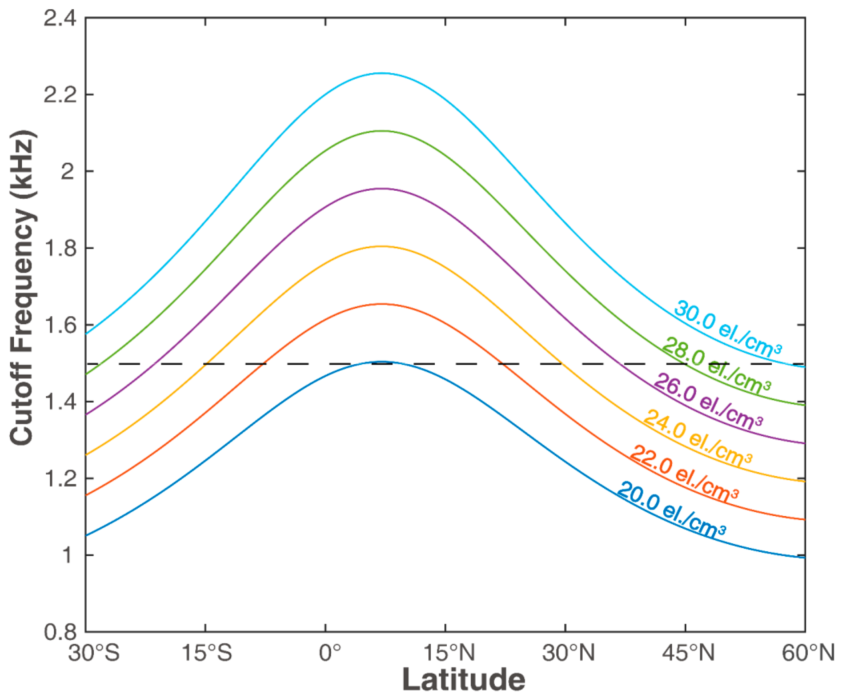The extrapolated tweek cut-off frequency showed daily and seasonal fluctuations, with a minimum of 1.62 kHz in summer and a maximum of 1.68 kHz in winter, with the corresponding reflection heights being 87 and 92 km [125]. At 90 km altitude and 120° E geographic longitude, the cut-off frequencies corresponding to different typical D-region electron densities at the reflection level and obtained using Equation (3) vary with geographic latitude, as shown in Figure 7 [125]. Because the geomagnetic field increases as the latitude increases, the electron cyclotron frequency at any fixed altitude increases, so that the tweeks reflected there have lower and lower cut-off frequencies. Thus, for a certain cut-off frequency, the reflection level is at its lowest altitude at the geomagnetic equator, where the geomagnetic field strength is smallest (near 8° E in this meridian). This is in accord with the results shown in Figure 6.

Although Maurya et al. [18] found many more tweeks at Allahabad, India, during the summer, when lightning activity is greatest during the year, Tiwari et al. [30] noted that the occurrence rate of tweeks at a receiver barely ~100 km to the east, at Varanasi, India, was only slightly higher in summer than in the other seasons, and that their duration was up to 30 ms. They were interpreted according to Equation (3), the electron density at the reflection level being 22 to 25 × 10⁶ m⁻³, with the reflection height generally being between 83 and 90 km for mode 1, and a few km higher for the higher-order modes (up to m = 10), where the electron density was up to ~140 × 10⁶ m⁻³. These values were shown to be consistent with radar and rocket data and with IRI [25] model values at similar latitudes.

Figure 3a of Reznikov et al. [44] indicated that the first mode cut-off frequency varied linearly from 1.70 kHz at Kp index of geomagnetic activity = 1 to 1.76 kHz at Kp = 5, even though the error bars are quite large. This can be interpreted as a slight lowering of the D-region ionosphere as magnetic activity increases. A specific study of tweeks observed at Selangor station in Malaysia (geomagnetic latitude −6.6° [23]) during the mild magnetic storm of 3 August 2010, with Dst reaching-65 nT, was carried out by Shariff et al. [126]. They found an increase of 9 km in the mean reflection heights of the tweeks from between 79 and 86 km on the geomagnetically quiet day of 29 August 2010 to between 88 and 96 km on the storm day. The ionospheric reflection height decreased from 85 km to 78 km during sunrise. The electron density at the reflection height on 3 August 2010 was between 22 and 25 × 10⁶ m⁻³ [126].

Ohya et al. [127] investigated long-term (1976–2010) variations of the reflection heights of tweek observations at Kagoshima, Japan. The results revealed the effects of the solar cycle on the nighttime lower ionosphere at low to middle latitudes. The tweek reflection heights on geomagnetically quiet days were analysed every month over three solar cycles; the average value was 96 km and the standard deviation was ± 3 km. A strong ~12-year periodicity was evident from their Figure 2, indicating a definite response to the solar cycle [127]. However, “clear correlations between the tweek reflection height and the sunspot number or the F10.7 index were not seen”. Further, they found that, during geomagnetic storms, the reflection height does not depend on the Dst value. On magnetically quiet days, no variation of reflection height with season was noted (their Figure 5) [127]. The tweek reflection height increased by a few km from evening to morning, and tended to be high from July to October (summer to autumn), and low in the spring, varying by a few km. They hypothesised that the variations in tweek reflection heights could be caused by different sources of D-region ionisation, including the geocorona, galactic cosmic rays, charged particle precipitation from the magnetosphere, and variations of neutral density in the lower thermosphere.

Zhang et al. [128] studied four nights of data with almost 50,000 tweeks recorded in Duke Forest, North Carolina, USA (geomagnetic latitude 45.1° [23]), during January 2010, and interpreted them using Equation (3). They found that the reflection height h_R1 lies between 85 and 93 km, with a local minimum between 01 and 02.30 local time; this corresponds to a local maximum in the electron density there [128], as also shown in Figure 7. On the most geomagnetically active of the four days, some hours after a moderate auroral substorm, with Dst being ~−35 nT, h_R1 was slightly higher than on the other days, at 88 to 93 km [128]. They also investigated the plasma density in the E- and F-regions on these days, using ionosonde data from Wallops Island, Virginia, and incoherent scatter radar data from Millstone Hill, in Massachusetts.

Using the data discussed so far, and shown in Table 1, I now ask the question: is there a significant variation of the first-order tweek reflection height with increasing geomagnetic latitude, θ, in the northern hemisphere? From Figure 7, I might expect a difference of ~(95–82) = 13 km between sub-auroral latitudes and the geomagnetic equator. This is quite a large difference between D-region reflection heights at different latitudes, brought about by different physical mechanisms. Figure 8 plots the mean values of h_R1, in km, against the geomagnetic latitude of the nine observing stations, in degrees. The equation of the best-fit straight line to these data points is

h_R1 = 0.153 θ + 82.1 km

(6)

The gradient of this best-fit line is 0.153 ± 0.095 km/degree of latitude and is certainly positive within ± one standard deviation. The intercept for θ = 0° is 82.1 ± 2.5 km; this intercept agrees well with its expected value. I note that at a geomagnetic latitude of 45.1° Figure 8 shows that h_R1 ~88 km, in good agreement with the observed mean value of 89 km [128].

The reciprocal of the gradient, i.e., the increase in the geomagnetic latitude corresponding to a rise in the reflection level by 1 km is 6.5°. For a range of stations between the geomagnetic equator and 50° geomagnetic latitude, the difference of reflection height levels could therefore be ~7.7 km, just more than half the expected value, and yet an appreciable variation of D-region reflection heights. This corresponds to the non-parallelism of the plates of the waveguide stretching from north to south being less than 0.1°. However, at dawn or dusk, the terminator causes a difference of reflection levels by ~20 km over two hours of local time, i.e., over 30⁰ of longitude or ~2100 km at middle latitudes. This creates a somewhat greater non-parallelism from east to west, by 0.2°, at these times.

It is important to state that the deviation of the slope of this best-fit line given by Equation (6) from zero is not statistically significant. The square of the correlation coefficient, r², has the value 0.27. In order to demonstrate a significant relationship between h_R1 and θ, a larger number of stations or a greater precision in determining h_R1 values from tweeks would be needed. Neither does Figure 8 show a 2 km decrease in the reflection level from 5° N to 15° N, as would be expected from [124].

Rodger et al. [129] considered what could happen to the lower ionosphere above an active thunderstorm. They showed that strong lightning-generated electromagnetic pulses at night can lead to significant, ~100% or even greater, increases in the electron density, with the largest increases at ~90 km altitude. Regions with significant decreases in electron density are also possible. Salem et al. [130] modelled changes in the night-time lower ionospheric conductivity by electrostatic fields produced by underlying thunderstorms. They found that, although the electron density is generally increased, the lower ionospheric conductivity can be reduced by at least one order of magnitude because the electron mobility is significantly reduced due to the electron heating effect. For a typical ionospheric density profile above an active thunderstorm, the resulting increases in the reflection heights of ELF and VLF waves were found to be 5 and 2 km, respectively [130].

The incoherent scatter radar at Arecibo, Puerto Rico, showed that sudden electron density changes during thunderstorm daytimes between 2012 and 2014 are, on average, different from those at other times [131]. These changes typically correspond to electron density decreases by ~7% in the D- and E-regions lasting for about one minute. The disturbances are different from those associated with the enhanced X-ray fluxes in solar flares, which tend to have longer durations (up to ~15 min) and most often show ~12% increases in the electron density [131]. Because the proportion of the waveguide that creates tweeks that is above the thunderstorms is small, it is likely that the electron density changes there have no detectable effects on the tweek spectrum or dispersion.

Kumar and Kumar [132] analysed the propagation of sub-ionospheric VLF signals from NWC and NLK transmitter stations monitored at Suva, Fiji, between December 2006 and December 2010 (during the solar minimum of solar cycles 23 and 24) and between January 2012 and December 2013 (moderate solar activity at the peak of solar cycle 24) to find D-region changes caused by solar flares. The amplitude and phase enhancements associated with solar flares were due to an increase in the electron density of the D-region; these were parameterised by h′ (the ionospheric reflection height) and β (the rate of increase in electron density with height) using LWPC version 2.1 modelling (see next section). A greater increase in β and a greater decrease in h’ were found during the low solar activity period compared with that during the moderate solar activity period, for the same class of flares. Greater changes in the values of β and h’ for strong flares in comparison with weak flares were noted under both low- and moderate-solar activity conditions.

Shao et al. [133] modelled the dispersive reflection of VLF radio waves generated by lightning discharges from a small night-time thunderstorm ~900 km from the radio receivers by the lower ionosphere. They found that the electron density was reduced by a factor of ~100 at ~82 km altitude within ~50 km from the storm. They ascribed this to enhanced electron attachment to oxygen molecules due to the lightning-generated electric fields, which had energised free electrons in the ionosphere [133].

Using a Finite Difference Time Domain (FDTD) method, Luque et al. [134] have recently modelled the enhanced electrical conductivity (see Section 1) of the ionospheric plasma, which is determined by electron-ion recombination, and the rings of light emitted by excited nitrogen molecules at ~85 ± 2 km altitude above an active thunderstorm with ~200 kA, negative cloud-to-ground discharges; these expanding rings are termed elves. They are one of the transient luminous events (TLEs) created above powerful thunderstorms, the others being red sprites, blue jets, and gigantic jets. An introduction to the properties of TLEs and their mechanisms, an active research area today, is provided by the book by Fullekrug et al. [135]; Inan et al. [136] and Köhn et al. [137] have brought the subject up to date. Kolmašová et al. [138] showed that elves can also be produced by positive cloud-to-ground lightning with high peak currents (>300 kA) and charge moment changes of ~300 C.km from a small-scale spring-time thunderstorm that occurred early in the night of 2 April 2017 in central Europe. Their Figure 5a shows in red only 2 ms of the waveform that they called “strong ionospheric reflections” of the sferic, which produced an elve (an expanding ring of light) at ~83 km altitude; this could be characterised as the “head” of a tweek having propagated over 800 km from the source.

With two years of data, Tatsuta et al. [139] studied three VLF transmitter signal amplitudes at seven receiving stations in Japan, i.e., for about 20 different paths, at high latitudes, mid-latitudes, and for north-south paths. Significant anomalies were found during geomagnetic storms for the high-latitude paths, due to auroral energetic electron precipitation. Because the occurrence rate of storm time anomalies was similar to that during geomagnetically quiet time periods, it was concluded that the ionosphere over the mid-latitude and north–south paths exhibits little change during geomagnetic activity. This is consistent with the results of tweek studies [127].

Summarising this section, the tweek reflection levels are ~5 km lower in summer than in winter according to [125]. The reflection level does not show a relationship with the storm time Dst index of geomagnetic activity [127], although it was a few km higher on the magnetically disturbed day out of the four days studied [128]. Neither do they show a relationship with the sunspot number nor the flux of solar radio emission at a wavelength of 10.7 cm, both of which are indicators of solar activity [126]. Whereas Figure 6 shows an appreciable increase in tweek reflection heights with increasing geomagnetic latitude in the northern hemisphere, Figure 8 shows that this is by 0.15 km/degree of latitude. In order to demonstrate a statistically significant variation, more stations and/or a better precision of measurement of cut-off frequencies are needed. The disturbed ionosphere above a thunderstorm, of up to ~100 km horizontal scale, is unlikely to have an observable effect on tweeks because they have propagated a large distance (~1000 km or more) from the thunderstorm. A positive cloud-to-ground discharge with a peak current > 300 kA, which produced a TLE at ~85 km altitude, termed an elve, caused strong ionospherically reflected signals resembling the “head” of a tweek [137].

7. Theoretical Models of Tweek Generation—Propagation in the Earth-Ionosphere Waveguide

Early work on this subject by Yamashita [140], Sukhorukov et al. [141,142], Ryubov [143], and Sukhorukov [144] proposed approximate analytical and numerical expressions to explain tweek formation as being due to a minimum in the frequency dependence of the attenuation of propagating waves near the waveguide cut-off frequencies; this is associated with the presence of the vertical component of the geomagnetic field.

Wait and Spies [145] considered the mode theory for the propagation of VLF waves in the spherical Earth-ionosphere waveguide and also for the flat Earth approximation. Their ionospheric model had an exponential variation with height for both the electron density and the electron-neutral collision frequency, and the effect of the Earth’s magnetic field was considered. Cummer [146] thoroughly reviewed this theory as formulated by Wait [147], Budden [9], and others, considering both analytical formulations and FDTD modelling. Figure 3b of [146] shows the horizontal magnetic field waveform of a signal propagating in the transverse electromagnetic (TEM) mode, which is similar to that propagating in a perfectly conducting parallel plate waveguide with a cut-off at 1.6 kHz. This waveform is shown for up to 5 ms after the causative lightning discharge that propagated 1000 km, computed using the LWPC that was developed at the US Naval Ocean Systems Center in San Diego, California [148]. This resembles a tweek waveform; modelled spectra [143] show that the amplitude of the wave is essentially zero at just ≤1.6 kHz.

Porrat et al. [149] have discussed theoretically the signal from a vertical electric dipole source in a parallel-plate Earth-ionosphere waveguide. For a perfectly conducting ionosphere, there exist transverse magnetic (TM) modes, with cut-off frequencies given by f_cm = mc/2h, as stated in the Introduction. For a lossy ionosphere, with a certain profile of electric conductivity, σ(h), following Wait and Spies [145], the propagating waves are quasi-transverse electric (QTE) modes having horizontal magnetic field components. Attenuation rates, in dB/Mm, can be calculated. They also presented, in their Figure 2, the average (over 150 s) spectrum from 0.5 to 5 kHz of the horizontal magnetic wave field at local midnight received in California. Besides peaks of ~26 dB at the fundamental and up to ~16 dB at harmonics of the mains electrical grid at 60 Hz, this displays a ~10 dB deep minimum at 1.7 kHz and a smaller ~3 dB minimum at 3.4 kHz, the first two cut-off frequencies of the TM waveguide. These are the minima, which are also seen directly in the tweek spectrograms. Fluctuations in the spectrum at night were also explored. They compared the calculated spectrum at midnight with the observed one; remarkably good agreement was found for h’ = 84 km and β = 0.6 km⁻¹, with the source-to-receiver distance being 1700 km [149].

Han et al. [150] discussed D-region electron density profiles derived by comparing measured daytime sferic spectra with the FDTD simulation results. In the FDTD simulations, they used the standard D-region electron density profile parameterisations of

N_e(h) = 1.43 × 10¹³ exp(−0.15h′) exp[(β − 0.15)(h − h′)] m⁻³

(7)

with h′ in km and β in km⁻¹, as given by Wait and Spies [145]. The parameter h′ controls the height of the electron density profile, whereas β controls the sharpness of the profile. Because the ionospheric conductivity at the reflection level, ~3 × 10⁻⁶ S/m (see Section 1), is much smaller than that of seawater, ~3 S/m [151], and smaller than that of typical rocks, ~10⁻³ S/m, the effects of ground conductivity variations along the VLF propagation path in the Earth-ionosphere waveguide, particularly on the attenuation of the radio waves, are generally small [149]. Said et al. [152] and Teysseyre et al. [153] have recently investigated these matters in some detail.

Cheng et al. [154] interpreted sferics recorded in North Carolina on 16 days in the summer of 2004 using Equation (7). With h’ = 83.8 km and β = 0.50 km⁻¹, that gave a realistic log-linear plot for N_e(h), with N_e increasing from 10⁶ m⁻³ at 73 km to 10⁹ m⁻³ at 92 km. They found that, over the 16 days, h’ varied from 82 to 85.5 km and β varied from 0.40 to 0.55 km⁻¹. For observations made in the summer of 2000, on a day with significant energetic electron (0.1 to 6 MeV) precipitation from the magnetosphere as measured aboard a satellite, h’ was lower, at 80 km. Because only daytime results were considered [150], tweek spectra were not computed. However, Cummer et al. [155] showed 20 ms of the waveform of a relatively strong (peak current 56 kA) negative cloud-to-ground lightning discharge over the midwestern USA recorded in California, its dynamic spectrogram, and the sferic spectrum, with a definite minimum at ~1.6 kHz, an attribute of a tweek. Xu et al. [156] have applied the ideas of [140] to D- and E-region ionisation profiles of the FIRI [42].

After the HT-HH volcanic eruption of 15 January 2022, Kumar et al. [157] observed VLF radio propagation anomalies at Suva, Fiji, some ~800 km away. Lasting ~40 min, these were interpreted using the LWPC code [148] as a reduction of h’ from a normal daytime value of 75 km to 72 km, with an increased sharpness of the lower D-region, with β doubling from 0.3 km⁻¹ to 0.6 km⁻¹. This meant that at 75 km altitude, the daytime electron density increased from 0.18 × 10⁹ m⁻³ to 1.3 × 10⁹ m⁻³. This was attributed to the enormous number of volcanic lightning discharges producing extra ionisation in the D-region [129,131] combined with the effects of acoustic gravity waves and Lamb waves generated by the volcanic explosion perturbing the mesosphere [63,76,77,157].

For the M = 6.9 earthquake in Samos, Greece, on 30 October 2020, Biswas et al. [158] used the LWPC [143] and the Wait and Spies [145] two-parameter description of the lower ionosphere to demonstrate that h’ was significantly raised, by >7 km, three and ten days before the earthquake. Are these changes precursors of the earthquake?

Shvets et al. [39] proposed a new way of using tweeks to estimate both the effective height of the ionosphere, having an exponential electrical conductivity profile [140], and the source-to-receiver distance. Multi-mode tweek waveforms were computed following the method of Porrat et al. [149] from which the effective ionospheric height was found to within a fraction of 1 km. They showed that, for a modelled tweek, where the source-receiver distance is ~1.6 Mm, h_R1 is 90.1 km, h_R2 is 89.1 km, h_R3 is 88.5 km, h_R4 is 88.1 km, and h_R5 is 87.7 km [39], consistent with the trend of decreasing reflection heights with increasing mode number, m, mentioned earlier (and see Figure 3). They found that, for observed tweeks [7], h_R2 was typically lower than h_R1 by 0.3 km in January (summer, for observations made at ~17° S) and by 0.9 km in April; h_R1 was 87.8 km in January (summer) and 90.0 km in April [39].

The most comprehensive theoretical study of tweeks and slow tails, together with a list of fundamental references to the subject, has been published by Nickolaenko et al. [159,160]. The propagation parameters of Earth-ionosphere waveguide modes were “calculated by using a full-wave solution in the form of the Riccati equation. According to these parameters, complex spectra of vertical electric and horizontal magnetic fields are obtained in the specified frequency band at a given distance from the source” [159]. (The Riccati equation is a first-order non-linear ordinary differential equation for which there is no general solution.) With a realistic electrical conductivity profile, the complex propagation constant was obtained. Curve 4 in their Figure 2b shows that at night its imaginary part, which determines the attenuation rate, reaches a broad minimum between ~1.5 and ~3.5 kHz for the m = 1 mode; this explains the tweek spectrum well. It is also consistent with the result shown in Figure 5, from [95].

They show that at ~2 kHz the attenuation is ~40 dB for a source-receiver distance of 1 Mm and ~80 dB for a separation of 2 Mm, whereas it is only ~0 dB at ~1 and ~5 kHz for these two distances [159]. Three different models for the spectrum of the lightning current moment, in kA.km.s, were considered. In these, “the current of the main breakdown in the lightning channel reaches its maximum in a few microseconds and then decreases over a time from tens of microseconds to several milliseconds. Peak current values are about 20–25 kA” [159]. These model discharges transfer several C from the cloud to the ground; more modern models transfer ~100 C from cloud to ground. Model tweek waveforms were presented in their Figure 6b for source-receiver distances, D, of 1, 2, 3, 4, 5, 6 and 10 Mm [159]. “Each pulse contains a high-frequency head part followed by a slow tail, which is a normal ELF burst”. The delay of the slow “tail” after the “head” increases as D increases from ~10 ms at D = 3 Mm to ~20 ms at 5 Mm and to ~35 ms at 10 Mm [159]. The slow tail contains the components of the electromagnetic wave with frequencies < 1 kHz [161].

For each of the four computed tweek “tail” waveforms, at different propagation distances, D, shown in Figure 9, reproduced from [160], measurements of the number of cycles were made for different 10 ms segments, as shown in

Table 3. Properties of tweek “tail” waveforms obtained from Figure 9.

Distance from Source (Mm)	Time After Source Impulse (ms)	Number of Cycles	Cut-Off Frequency (kHz)	Peak Amplitude (Arbitrary Units)
1	5–15	17	1.7	0.19
2	10–20	18	1.8	0.05
3	15–25	18.5	1.85	0.015
4	20–30	19	1.9	0.005

. From these, the frequency, which is the cut-off frequency, is simply obtained. As the source-to-receiver distance, D, increases, so does the cut-off frequency, corresponding to a lowering of the ionosphere. As D increases, the wavefronts of propagating QTE waves just above f_R1 become more nearly perpendicular to the Earth’s surface. This result complements the result derived from tweek observations [39] that the cut-off frequency increases as the mode order increases.

Summarising this section, the theory for the modes propagating in the Earth-ionosphere waveguide is based on the work of Budden [9], amongst others, and the formulation of Wait and Spies [145], which uses the ionospheric height parameter h and the steepness of the gradient parameter β. A complementary formulation is provided by Nickolaenko et al. [160]; it uses an empirical conductivity profile through the atmosphere and the Riccati equation to solve for the modes. Both methods compute tweek waveforms and permit the source-receiver distance to be found. Following the HT-HH volcanic eruption of 15 January 2022, the ionosphere was disturbed; changes to the h and β parameters were deduced [161]. Changes in these parameters several days before a large earthquake have been claimed [158].

8. Discussion

I now briefly discuss some issues that arise from the results of the research that has been conducted on tweeks and related topics in the last 25 years and what could be done to make progress in the future.

Opinions vary as to whether there is a significant seasonal variation of h_R1. Likewise, opinions differ about a possible variation of h_R1 with the three-hourly index of geomagnetic activity. After some geomagnetic storms (increasingly negative Dst values), h_R1 is found to decrease by a few km; this could be caused by extra D-region ionisation due to energetic charged particle precipitation from the magnetosphere. After other geomagnetic storms, h_R1 increases by a few km. Thus, further studies are required to obtain a definitive result that could be important in the context of space weather effects on the Earth’s upper atmosphere.

Some hours, days, or even some weeks before a large earthquake, anomalous changes (either increases or decreases) in the D-region ionosphere, in the electron density or temperature of the topside ionosphere at ~500 km altitude, and in the TEC of the ionosphere have been claimed by many different authors. The statistical significance of these results is often debatable. These studies do not conform to the expectation based upon [95] that the precursor anomalies would only occur in the four hours before the earthquake. Because of the practical importance of this issue for human society, definitive research is needed. Several different physical mechanisms to account for such claims have been proposed, but none is without its detractors. Various mechanisms whereby processes operating in the Earth’s surface, above it, and in the ionosphere before large earthquakes have been considered [113,119,120,122]. No one mechanism is totally convincing, but acoustic gravity waves (AGWs) are likely to be important. Because the signal associated with such a mechanism has to pass upwards through the D-region, tweeks could be a way of studying the causative mechanism(s).

Although FIRI [42] representations of D-region parameters may generally be considered to be better than those of the IRI [25], there is a notable difference between tweek-derived profiles and FIRI ones. Rather than attributing this to limitations of FIRI, it is possible that shortcomings of the methods of tweek inversion or of propagation modelling may be the cause. In order to make progress, an international campaign could be planned and implemented to observe tweeks on specified days, in different seasons and phases of the solar cycle, at stations of different latitude; it would also be beneficial to geolocate the lightning discharges causing the tweeks by observing their azimuthal bearings as observed from the different stations.

In a very recent review, Hayakawa [162] has demonstrated several scientific topics and their underlying physics that can be studied using VLF/LF radio observations of both tweeks and transmitter signals; many of these have been mentioned here. How the ionosphere may be perturbed due to earthquake precursor activity in the Earth, the modulation of VLF/LF data by atmospheric gravity waves, and satellite observations of ground-based VLF/LF transmitter signals are considered in that review [162]. These topics, as well as several other related ones, have been considered in Section 5.

9. Conclusions

Here I provide a synthesised summary of the main geophysical points and the reasons for them, which can be concluded from studies of the observed spectrograms of tweeks, their spectra, and their waveforms, together with interpretations of their dispersion using mode theories of their propagation in the Earth-ionosphere waveguide. I also draw attention to some possible and important future studies.

The best quality tweeks are observed at night-time. Their simplest interpretation is that the waveguide cut-off frequency is f_cm = mc/2h, where m is an integer, c is the velocity of light in free space, and h is the height of the ionosphere. For the value f_c1 = 1.8 kHz, h_R1 = 83 km, where N_eR, the electron density at the reflection level, h_R1, is ~27 × 10⁶ m⁻³. The duration of the m = 1 tweek is up to ~40 ms at night, but only ~12 ms by day.

There is a small discrepancy between f_cm values obtained from tweek spectrograms and those extrapolated from these by some mode-fitting algorithm. This leads to higher h_Rm values for the mathematically extrapolated tweek spectrograms, which could explain some of the scatter of h_R1 values shown in Table 1 and Figure 8. When several modes are apparent, h_Rm is a few km above h_R1. Therefore, an approximate profile of the lower D-region can be obtained when m ≥ 2; further studies of these profiles, and comparisons with those obtained using mode theories, or with ionospheric models such as IRI or FIRI, would be desirable. It is noteworthy that Figure 3 and the results presented in [39] show the opposite result; my opinion is that the latter is correct. h_R1 generally rises by a few km after sunset towards local midnight and on towards dawn. This is understandable in terms of the loss of D-region ionisation by recombination when the flux of solar radiation at night is much less than during the daytime. No clear systematic variation of h_R1 with season or geomagnetic activity has been found at different stations at different latitudes.

Tweeks have been observed during six solar eclipses; h_R1 increases from onset to totality by up to ~7 or 8 km and then falls by the same amount when the eclipse ends. The conclusions derived from tweeks concerning propagation in the Earth-ionosphere waveguide are reinforced by complementary studies of the amplitude and phase of signals from ground-based VLF transmitters used for communication with submarines. During and just after the explosion of the HT-HH volcano, which occurred on 15 January 2022, the number of atmospherics generated by volcanic lightning was several times the usual rate generated by thunderstorms [72]. Tweeks were not observed because the eruption occurred during the local afternoon.

DEMETER satellite observations show a very clear association between a reduction (by 4 to 6 dB) of the 1 to 2.4 kHz natural signal intensity within the preparation zone of a large earthquake some hours before the earthquake strikes [95]. Figure 5 shows that during the two days before a major shallow earthquake (M ≥ 5) the only significant change is a reduction of the intensity of ~1 to 3 kHz noise in the time interval up to 4 h before the earthquake [95]. My opinion is that this is an important finding. This result could be ascribed to a lowering of the D-region by ~2 km, which makes the Earth-ionosphere waveguide more attenuating and so reduces the intensity of up-going fractional hop whistlers—see [163]. The lowering of the ionosphere may be associated with an increase in the electrical conductivity of the lower troposphere due to an additional ionisation source of air molecules at the Earth’s surface prior to earthquakes [101]. It would be worthwhile to investigate tweeks in this context.

Figure 6 shows another DEMETER result [97], that h_R1 is unusually low at and near the geomagnetic equator (over the Atlantic Ocean) and at sub-auroral latitudes (L ~3); h_R1 rises appreciably from ~5° geomagnetic latitude to ~50° geomagnetic latitude. This could be explained by the dependence of the solar zenith angle on geographic latitude. Figure 8 shows a plot of the mean h_R1 northern hemisphere data for the different receiver stations presented in Table 1 against geomagnetic latitude, up to 50°. Whilst there seems to be an increasing trend, the deduced latitudinal change in D-region reflection heights has not reached a value that is statistically significant. Further research is required on this topic.

Above an active thunderstorm, the lower ionosphere is likely to be drastically changed. However, because this region is only a small part of a tweek’s propagation path, it is unlikely to change the characteristics of the tweeks. After a very high current lightning discharge, an expanding ring of light lasting a few ms at ~85 km altitude, i.e., an elve, can occur. In this case, “strong ionospheric reflections” of the radio signal have been observed [138]; at a propagation distance of ~800 km, these could be termed the “heads” of tweeks. It would be worthwhile to study tweeks generated by the strongest lightning discharges, which produce TLEs, and to geolocate them using lightning network observations. Then the propagation distance D could be compared with the value expected from waveguide mode calculations.

The theoretical interpretation of tweeks is based upon considerations of the modes propagating in the Earth-ionosphere waveguide [146,149], and the formulation of Wait and Spies [145] which uses an ionospheric height parameter h and the steepness of the D-region gradient parameter β. A complementary formulation is provided by Nickolaenko et al. [160], which uses an empirical conductivity profile through the atmosphere and the Riccati equation to solve for the modes. Both methods compute tweek waveforms and permit the source-receiver distance to be found. The “head” of a tweek is linearly polarised. The polarisation of the “tail” of a tweek has been investigated [5,39]; it propagates in the Earth-ionosphere waveguide as an X-mode, specifically a quasi-transverse electric (QTE) mode in which the wave electric field is primarily, but not entirely, transverse (i.e., perpendicular) to the propagation direction. At frequencies just above the cut-off frequencies, the attenuation rate is very small, <1 dB/Mm. In the presence of the horizontal component of the geomagnetic field, east-to-west propagating waves suffer less attenuation near the cut-off frequency than west-to-east propagating waves [7,20]. Tweeks propagating up into the ionosphere as upgoing whistlers, and fractional hop whistlers such as those observed aboard DEMETER [98] and CSES [164], are right-hand circularly polarised O-mode waves. Their possible association with earthquake precursor activity would be an exciting research topic.

I hope that this article may stimulate further research on tweeks and related phenomena and lead to an improved understanding of the important topic of the coupling between lithospheric, atmospheric, and ionospheric processes.