Validation Design Governs the Apparent Performance of Machine Learning Calibration for Low-Cost Optical Particle Counters: A PM₁ Study

Abstract

Low-cost optical particle counters (OPCs) are increasingly deployed to resolve spatial variability in indoor particulate matter levels that sparse reference networks cannot capture, but their output requires field calibration. We evaluated three co-located low-cost sensors against the means of reference nephelometers over seven discrete co-location runs of 20–33 h each, conducted between June and September 2022. We used 1-min and hourly aggregations and six calibration models (multiple linear regression, support vector regression, random forest, gradient boosting, XGBoost, and LightGBM). Reference PM₁ averaged 8.4–9.2 µg m⁻³. Factory-calibrated sensor output underestimated reference values by 5.3–6.1 µg m⁻³, with an RMSE of 6.5–7.6 µg m⁻³, representing 74–82% of the reference mean. Under a conventional random 80/20 hold-out, tree ensembles reached R² = 0.86–0.89 at 1-min resolution. When progressively stricter designs (day-blocked, leave-one-run-out, forward chaining and chronological hold-out) were applied to the same data and models, R² fell sharply from random to day-blocked to run-blocked validation and remained near or below zero under forward chaining and chronological hold-out. Calibration remained worthwhile, reducing prospective RMSE by 22–48%, but the calibrated slope fell to 0.18–0.44, so real variation was substantially compressed. Validation design accounted for 63–91% of the spread in R², while algorithm choice accounted for 3.6–10.6%. We conclude that reported machine learning calibration performance is governed more by validation design than by algorithm choice.

1. Introduction

Exposure to airborne particulate matter (PM) is associated with 4.2–8.9 million premature deaths globally per year, primarily through lung cancer, ischemic heart disease, stroke, and chronic obstructive pulmonary disease (COPD) [1,2,3]. PM is conventionally classified by mean aerodynamic diameter into coarse (<10 µm, PM₁₀), fine (<2.5 µm, PM_2.5), sub-micron (<1 µm, PM₁), and ultrafine (<0.1 µm, PM_0.1) fractions. As particle size decreases, depth of deposition increases: PM₁₀ is deposited in the upper respiratory tract, PM_2.5 reaches the bronchioles and potentially the alveoli, PM₁ penetrates into the lower lobes and alveoli, and PM_0.1 can cross the air–blood barrier to enter systemic circulation [3,4].

Due to the present air quality standards, studies have predominantly focused on PM_2.5 and PM₁₀, and the relative scarcity of research on PM₁ is recognized as a cause for concern [4]. While studies on PM₁ have mostly addressed long-term health outcomes—including hypertension, cardiovascular diseases, and autism spectrum disorder—short-term exposure has been associated with cardiovascular mortality as well as emergency hospital admissions due to pneumonia and COPD [5,6]. Currently, there are no international or national ambient or indoor air quality standards established for PM₁.

Microenvironments exhibit high spatiotemporal variability of fine particle concentrations [7,8], which complicates mapping and requires dense monitoring networks. Because reference-grade indoor monitors are expensive, networks composed of them are rare. Low-cost sensors (LCSs) offer a means to overcome this limitation [9,10,11,12]. Although the U.S. Environmental Protection Agency (EPA) initially defined LCSs as devices priced below 2500 USD [13], the term is currently applied to units under 100 USD [14,15].

LCSs for PM use light-scattering optical particle sensors, which are categorized into nephelometers, which measure particle ensembles, and optical particle counters (OPCs), which detect individual particles and report both count and size information [16]. Optical methods do not directly measure mass; instead, mass is derived from scattering data via calibrations that assume a specific particle density and refractive index [17]. OPCs provide size-resolved information while remaining among the most affordable instruments in their class. Both gas and particle sensors are susceptible to interference from relative humidity (RH), temperature, and other ambient conditions [18,19]. High RH induces hygroscopic particle growth, leading to an overestimation of dry mass and complicating the retrieval of size fractions [20].

Because the relationship between sensor response and reference concentration is non-linear and condition dependent, machine learning (ML) has become the standard approach for field calibration, with comparative studies being widely explored in recent years. However, few studies address PM₁ specifically [14,21,22,23]; most focus on PM_2.5 [11,24,25,26,27,28,29,30,31,32,33,34], reflecting the 2021 U.S. EPA performance-testing protocol, which focuses on sensors for fine PM [35]. That protocol frames linear evaluation around the Pearson correlations between sensor and reference values, followed by the coefficient of determination (R²) and root mean square error (RMSE) of simple linear regression. Wang et al. [36] developed a multi-input multi-output calibration system. Comparing random forest (RF), multiple linear regression (MLR), k-nearest neighbors (KNN), back-propagation (BP) networks, and a network optimized with a genetic algorithm (GA-BP), which achieved R² values between 0.68 and 0.99 for PM_2.5 and PM₁₀. Taştan [33] evaluated eight algorithms (linear regression [LR], KNN, AdaBoost [AB], gradient boosting [GB], support vector machines [SVM], and stochastic gradient descent [SGD]) on an internet of things (IoT)-based platform, reporting R² = 0.970 with RMSE = 2.12 μg/m³ for PM_2.5 using KNN. Koziel et al. [22,23] presented an artificial neural network combined with affine response correction, reporting correlation coefficients of 0.86 for PM₁ and PM_2.5, and 0.76 for PM₁₀. The authors subsequently extended this approach using time-series alignment to compensate for lags between the sensor and reference values. Feng et al. [34] conducted a long-term field evaluation of four ML models (MLR, SVR, RF, and extreme gradient boosting [XGBoost]), reporting that the RF model outperformed the other ML models. Furthermore, SHAP analysis applied to interpret model behavior revealed that relative humidity exerted a greater influence on calibration performance than dew point and temperature.

Results indicating low performance in comparative ML calibration experiments were also reported recently. Villarreal-Marines et al. [25] analyzed a full year of PM_2.5 data obtained from light-scattering sensors and found that XGBoost elevated the regression performance from a baseline of R² ≈ 0.3 to R² ≈ 0.5, which was considered to be low compared to other studies, and attributed the discrepancy to local climate and emission conditions. Evaluating low-cost sensors with ML models, Attey-Yeboah et al. [26] achieved R² values ranging from 0.18 to 0.27 and reported that seasonal variability strongly influenced model performance, with dry-season models substantially outperforming wet-season models. Consequently, the reported R² values for the ML calibration of low-cost PM sensors span roughly from 0.18 to 0.99. A portion of this dispersion reflects differences in sensor design, pollutant type, concentration range, and climate.

Sensor-reference comparison datasets constitute time series with strong autocorrelation: consecutive observations at a 1-min resolution are nearly identical. When such data are split into random training and testing sets—the default approach in most of the studies cited above, including our own prior work [37]—temporally adjacent observations are distributed across both sets. Rather than learning a transferable relationship between the sensor response and the reference concentration, a flexible learner can achieve low test error rates simply by interpolating within the temporal neighborhood of each test observation. The observations on seasonal transfer by Attey-Yeboah et al. [26] and temporal deterioration by Bachechi et al. [21] are consistent with this concern, and blocked cross-validation is well established as an appropriate solution for structured data in other domains [38,39].

This study systematically evaluates model performance by comparing traditional random splitting with out-of-time validation schemes for OPC calibration. Furthermore, to characterize the underlying sensor–reference dynamics, we investigate the effects of temporal aggregation and predictor variables on calibration performance, thereby assessing variations in quality of PM₁ data generation. By deploying six calibration algorithms across two temporal resolutions and under five validation frameworks, we benchmark three Alphasense OPC-R2 sensors—a model for which, to the best of our knowledge, no peer-reviewed calibration study has been published—against reference nephelometers.

2. Materials and Methods

2.1. Instrumentation

The sensor evaluated is the Alphasense OPC-R2 model (Alphasense Ltd., Great Notley, UK). Like other optical particle counters, the OPC-R2 measures the light scattered by individual particles passing through a laser beam within an airflow; these measurements determine particle size and number concentration via calibration of the scattered light intensity grounded in Mie theory. Particle mass loadings for PM₁, PM_2.5, and PM₁₀ are calculated from size spectra and concentration data by assuming a particle density and refractive index (RI); number concentrations are converted to mass concentrations through an established factory calibration referencing the European Standard EN 481. Default settings assume two weighting indices, a density of 1.65 g mL⁻¹, and a refractive index of 1.5 + i0. As with most commercial OPCs, all particles are assumed to be spherical regardless of their actual shape and are assigned a spherical equivalent diameter, whereas factory calibration employs polystyrene latex (PSL) spheres of known diameter and RI.

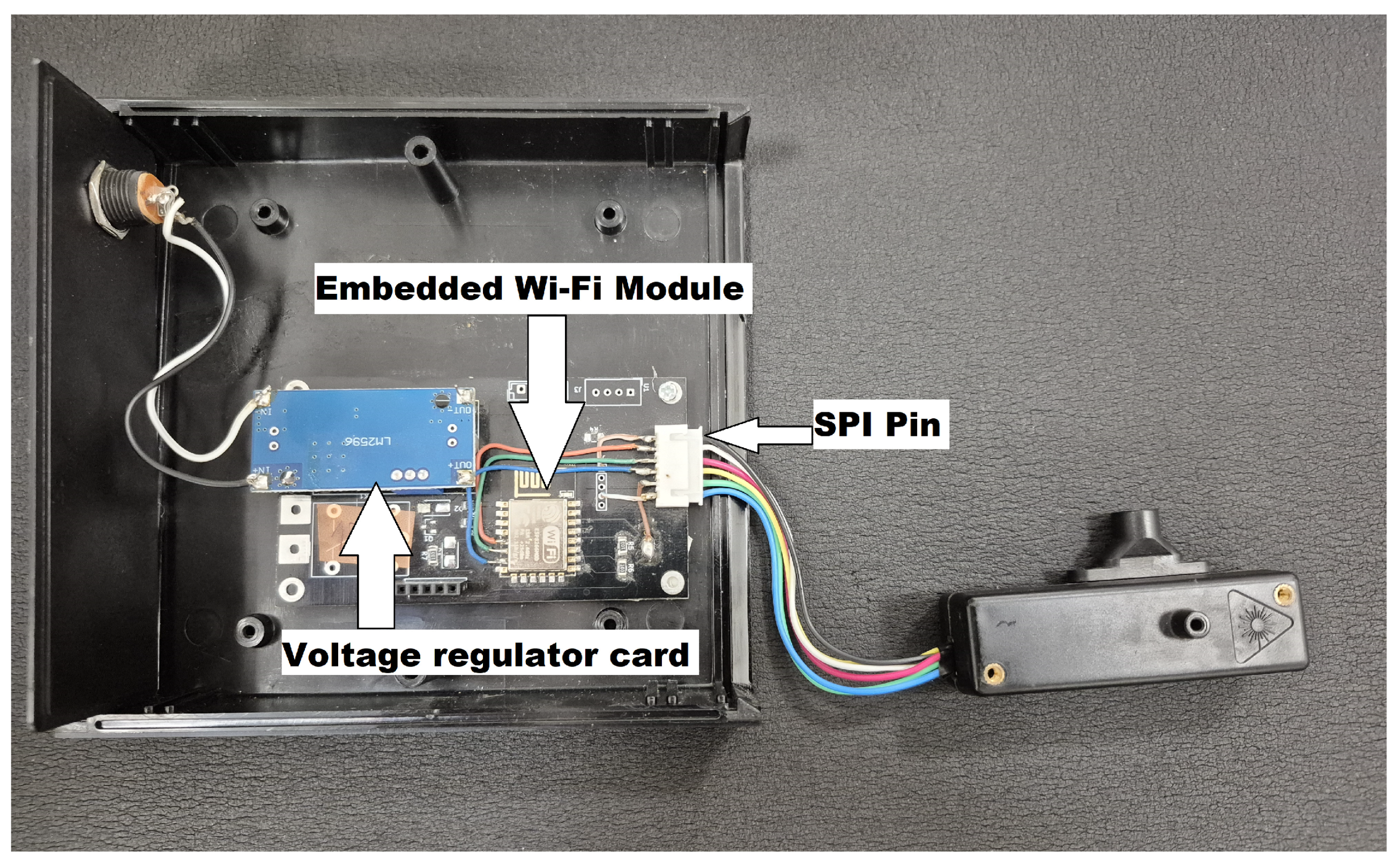
Because the manufacturer’s data logging software was designed for a single sensor connected to a personal computer, a custom microcontroller-based data acquisition system was developed for concurrent multi-sensor and long-term operation. The sensor is interfaced with the microcontroller (WEMOS/LOLIN, Shenzhen, China) via an SPI protocol and powered with a regulated 5 V supply through a voltage regulator board. The assembled system architecture is shown in Figure 1. Histogram data are logged at 10 s intervals using manufacturer-provided control code that reads the device serial number and information string, initializes the sensor, retrieves configuration parameters, and manages operation via a watchdog timer. The acquired data were transmitted over Wi-Fi using HTTP to a storage network, enabling real-time synchronization with the reference instrument.

Three pDR-1500 (Thermo Fischer Scientific, Waltham, MA, USA) units served as the reference monitors. The pDR-1500 is a nephelometric monitor that uses a light-scattering detection configuration optimized for the respirable fraction of airborne dust, smoke, and mist. To mitigate measurement errors under high RH conditions, it incorporates integrated temperature and RH sensors and maintains volumetric flow control via digital feedback derived from an internal barometric pressure sensor, a temperature sensor, and calibrated differential pressure measurements across a precision orifice. Each unit was operated with the SCC 1.062 “Blue” sharp-cut cyclone at a volumetric flow rate of 3.5 L min⁻¹, the combination that provides a 1 µm 50% aerodynamic cut point, so that PM₁ is measured directly rather than derived from a larger size fraction. The instrument converts scattered light to mass assuming a refractive index of 1.54 + i0 and a particle density of 2.6 g mL⁻¹, against 1.5 + i0 and 1.65 g mL⁻¹ for the OPC-R2.

At the start of campaign, the zero point of each pDR-1500 was re-established by supplying particle-free air through the zeroing filter kit supplied with the instrument. Flow was verified against an external manual flow meter at six set points spanning 1–3.5 L min⁻¹ and the instrument reading was adjusted accordingly; the procedure was repeated a second time after the first calibration left residual disagreement between units. Instrument clocks were synchronized to the second before each co-location run. After the second flow calibration over 24 hours, 1-min PM₁ readings from the three units correlated at r = 0.88–0.97 and hourly means at r = 0.89–0.98. Over the co-location campaign reported here, pairwise hourly agreement was r = 0.77–0.94. Sensor–reference cross-correlation was flat within ±15 min, with no consistent optimal lag across runs (maximum gain of 0.14 over lag zero), so records were matched on clock time at 1-min resolution.

Gravimetric verification was performed using each instrument’s own 37 mm glass fiber filter, Whatman Grade GF/C (Cytiva, Marlborough, MA, USA). Filters were conditioned in a desiccator for at least 24 h before and after sampling and weighed on a balance (Shimadzu Corporation, Kyoto, Japan) of 0.01 mg resolution, and the resulting gravimetric concentrations were compared with the time-weighted average photometric concentrations, and with a co-located low-volume sampler fitted with a Harvard impactor (Air Diagnostics and Engineering Inc., Harrison, ME, USA) PM₁ inlet, in three parallel experiments of 6, 20 and 24 h. Photometric and gravimetric values differed by 1.8–2.6 µg m⁻³ and a paired t-test did not detect a significant difference (n = 3; p = 0.18–0.37). Given the small number of paired samples this comparison has limited statistical power, and no gravimetric correction factor was applied to the data analyzed here.

The reference value used throughout this study is the arithmetic mean of the three reference monitors. It is therefore a co-located photometric transfer standard whose agreement with a gravimetric method has been checked but not enforced, and the agreement statistics reported below are relative to that standard rather than to a gravimetric reference method. Throughout, PM₁ denotes mass concentration (µg m⁻³) and the OPC-R2 derives it from its number-size histogram, whereas the pDR-1500 derives it from ensemble light scattering.

2.2. Experimental Design

The sensors and reference instruments were co-located in the Environmental Engineering Laboratories of the İzmir Institute of Technology, in a room of 6.10 m × 11.4 m with a ceiling height of 3.80 m, ventilated from ceiling-mounted supply diffusers at approximately six air changes per hour. Each pDR-1500 was positioned directly in front of one OPC-R2 unit at the minimum separation required to prevent mutual interference, and raw data were recorded at a 1-min temporal resolution. The three OPC-R2 sensors monitored during the campaign were designated as S1, S2, and S3.

Measurements were not continuous. Data were acquired in discrete co-location runs of approximately 20–33 h, each beginning in the afternoon and continuing through the following day. Runs were scheduled specifically on days without laboratory activity: most began on a Monday, after a weekend during which the room was closed and its aerosol allowed to stabilize, and access was restricted for the duration of each run. This design isolates the sensor–reference optical comparison from occupant-generated source events, at the cost of a correspondingly narrow concentration range.

Sensor S3 was operated over seven runs between 10 June and 1 September 2022, S2 over six and S1 over five, all of the latter within 1 August–1 September 2022. After quality assurance these yield 6811, 8939 and 9933 one-minute records for S1, S2 and S3, corresponding to 127, 161 and 183 hourly means spanning 10, 12 and 14 calendar dates, respectively. Within-run data coverage was 86–96%. Individual runs lasted 19.4–32.8 h for S1, 23.5–32.8 h for S2 and 20.1–32.8 h for S3. Because each run began in the afternoon (12:20–19:32) and ended the following day (12:43–21:10), every calendar date contains only part of a day: approximately 4.5–11.7 h on the first date of a run and 12.7–21.2 h on the second. Each run is identified below by its starting date. Consecutive runs are separated by 1.3–17 d for S1 and S2; for S3, the June run leads the August series by 51 d.

Because the operational periods of the three sensors were not identical, each sensor was analyzed over its own set of runs against the same three-unit reference mean, and direct inter-sensor concentration comparisons were not performed.

2.3. Quality Assurance

Prior to attempting any calibration study, raw sensor data were screened using a set of criteria addressing data acquisition errors, instrument operational ranges, and statistical outliers. All quality assurance (QA) criteria were applied identically across all three sensors.

Sensor timestamps were rounded to a 1-min temporal resolution, and duplicate records were removed; subsequently, records with missing sensor outputs were excluded (affecting 982 records [12.3%] for S1 due to data acquisition interruptions, while S2 and S3 remained unaffected). Records where sensor temperature or relative humidity (RH) were reported as zero were discarded as data acquisition errors, as these also yielded physically impossible dew points of −83.4 °C. Observations recorded when the reference RH exceeded 70% were excluded to mitigate the strong non-linear effects of hygroscopic growth on the optical response under high humidity conditions.

An outlier filter was applied independently to each sensor. A modified z-score recommended by Iglewicz & Hoaglin [40] was computed on the sensor PM₁ values using the formula z = 0.6745 (x − median)/MAD (where MAD denotes the median absolute deviation), and records with z > 3.5 were identified as outliers [41]. Because the consistency constant assumes approximate normality, while indoor PM₁ concentrations are strongly right-skewed, the criterion was evaluated on log-transformed PM₁ values [42]. Data were evaluated by reducing the sensor PM₁ skewness with log transformation from 4.4–52.7 to a range of −0.3 to 1.3. When applied to non-transformed data, 1.9% to 7.0% of the observations were removed as outliers, whereas outlier filtering on the log scale excluded 1.5%, 0.5%, and 1.3% of the data for S1, S2, and S3, respectively. The duplicate and acquisition-failure checks removed only one, one and four records from S1, S2, and S3, respectively; whereas the exclusion of observations above 70% at reference RH accounts for 67, 92 and 93 records (approximately 1% per sensor). Cumulative data losses, including missing records, were 14.5%, 1.55%, and 2.22%, leaving 6811, 8939, and 9933 1-min records corresponding to 127, 161, and 183 hourly averages, respectively (

Table 1. Record counts through the quality-assurance procedure.

Step	S1	S2	S3
Raw records	7968	9080	10,159
After removal of missing sensor output	6986	9080	10,159
After duplicate removal	6986	9080	10,158
After acquisition-failure removal	6985	9079	10,155
After RH >70% exclusion	6918	8987	10,062
After outlier removal	6811	8939	9933
Cumulative removal (%)	14.5	1.55	2.22
Hourly means available	127	161	183

). The sensitivity of the results to both exclusion steps was assessed by repeating the random, day-blocked and leave-one-run-out analyses without the RH filter, without the outlier filter and without either filter (Section 3.5).

2.4. Temporal Aggregation

Analyses were performed at two temporal resolutions. The original 1-min records constitute the primary analysis, providing between 6811 and 9933 observations per sensor to satisfy the large dataset requirement of machine learning calibration models. Zhu et al. [39], propose a sample size-to-feature ratio (SFR) as a rough adequacy check; the 1-min datasets yield SFR values of 1703, 2235 and 2483 and the hourly datasets 32, 40 and 46. We report these for completeness but do not treat the ratio as evidence of adequacy because it carries no clear interpretation for the non-linear models evaluated here. Hourly arithmetic means were calculated as a secondary, interpretative analysis. Hourly aggregation reduces noise and ensures comparability with published values in the literature; however, it reduces each sensor dataset to between 127 and 183 observations. The hourly datasets are small in absolute terms, and hourly results were therefore used to characterize relationship dynamics and to permit comparison with published values, not for model selection.

2.5. Predictor Variables

Four predictors—all measured directly by the sensor itself—were utilized: PM₁, temperature, relative humidity, and dew point. Dew point was included because it serves as an effective proxy for hygroscopic growth [43]. Although the PM_2.5 and PM₁₀ channels of the sensor were initially considered as additional predictors, they were excluded because they do not represent independent measurements; rather, they constitute cumulative mass fractions derived from the same underlying histogram. The correlations between PM₁ and PM_2.5 in the sensor data ranged from 0.847 to 0.926. In six-predictor models, variance inflation factors (VIF) reached 26.7–38.4 for PM₁ and 36.1–91.8 for PM_2.5, indicating severe multi-collinearity [44]. Furthermore, incorporating both PM fractions into the model yielded no performance improvement. Nevertheless, six-variable models are also reported in the Section 3 for comparative purposes. Meteorological variables measured by the reference instruments were likewise excluded, as they would be unavailable at deployment sites and their inclusion would yield a model unsuitable for field application.

2.6. Calibration Models

Following the recommendation of Zhu et al. [39] to benchmark machine learning (ML) outcomes against at least one statistical model, six regression models—comprising one statistical method and five machine learning algorithms—were evaluated.

Multiple linear regression (MLR) models the relationship between multiple independent variables and a single dependent variable:

Y = β₀ + β₁X₁ + β₂X₂ + ⋯ + β_nX_n

(1)

where Y is the dependent variable, β₀ is the intercept, β1, …, βn represent the coefficients of the independent variables X₁, …, X_n and є is an additive error term, omitted from Equation (1) for simplicity.

Support vector regression (SVR) extends the support vector framework from classification to regression tasks [45,46]. The prediction is expressed as

f(x) = w^⊺Φ(x) + b

(2)

where Φ(x) maps the predictors into a higher-dimensional feature space, w is the weight vector, and b is the bias term. The parameters are obtained by minimizing a combination of model flatness and deviations falling outside an є-insensitive tube around the fitted function [47]:

$$\underset{w,b,\xi ,{\xi }^{*}}{\min }{\displaystyle \frac{1}{2}}{‖w‖}^2+C{\sum }_{i=1}^n({\xi }_i+{\xi }_i^{*})$$

(3)

subject to the constraints for each observation i = 1, …, n:

$$y_i-f\left(x_i\right)\le ϵ+ {\xi }_i , {\xi }_i \ge 0 , f\left(x_i\right)- y_i \le ϵ+{\xi }_i^{*} , {\xi }_i^{*} \ge 0$$

(4)

These two inequalities specify the same requirement applied in both directions: the prediction can lie at most є below the measured value and at most є above it. Observations satisfying both conditions lie inside the є-insensitive tube and contribute nothing to the objective function. When an observation falls outside the tube, one of the two slack variables becomes positive and records the extent of the violation beyond є (ξi when the model underpredicts, and ξi* when it overpredicts). Consequently, Equation (3) balances two competing objectives: the first term favors a flat function by keeping ‖w‖ small, whereas the second term penalizes the total distance by which observations escape the tube. The constant C governs the trade-off between them; thus, a large C forces the function to fit the training data tightly, while a small C allows a smoother fit with greater deviations. The mapping Φ(x) is never explicitly evaluated; instead, it is replaced by a kernel function. For this study, a radial basis function (RBF) kernel was employed:

$$K\left(x_i,x_j\right)=\mathit{exp}\left(-\gamma {‖x_i-x_j‖}^2\right)$$

(5)

where γ controls the kernel width and consequently the smoothness of the fitted function.

Random forest (RF) regression constructs decision trees from randomly selected bootstrap samples and subsets of predictor variables [48]; as a result, each tree differs in structure and in the features utilized. This enhances diversity among the trees and mitigates the risk of overfitting. The final prediction is calculated as the average of the individual tree predictions:

$$\widehat{y}={\displaystyle \frac{1}{n}}{\displaystyle \sum _{j=1}^n}{\widehat{y}}_j$$

(6)

where n denotes the number of trees, which was set to 200 in this study.

Gradient boosting regression (GBR) differs from RF in that trees are grown sequentially rather than independently, with each tree fitted to the errors of the existing ensemble [49]. Starting from a constant initial prediction, the model at the m-th stage is expressed as

F_m(x) = F_m−1(x) + vh_m(x)

(7)

where v is the learning rate, and h_m (x) is a regression tree fitted to the pseudo-residuals, with L representing the squared error loss:

$${\tau }_{\mathit{im}}=-{\left[{\displaystyle \frac{\partial L\left(y_i, F\left(x_i\right)\right)}{\partial F\left(x_i\right)}}\right]}_{F\left(x\right)=F_{m-1\left(x\right)}}$$

(8)

For squared error, the pseudo-residual reduces to the ordinary residual y_i-F_m−1(x_i); thus, each successive tree models the variance left unexplained by the ensemble up to that point.

XGBoost (XGB) implements the same additive framework but optimizes a regularized objective function wherein model complexity is explicitly penalized [50]:

$$\mathcal{L}=\sum _{i}L\left(y_i,{\widehat{y}}_i\right)+\sum _k\mathsf{\Omega }\left(f_k\right) , {\mathsf{\Omega }}_{\left(f\right)}=\mathsf{\gamma }T+{\displaystyle \frac{1}{2}}\lambda {‖w‖}^2$$

(9)

where T is the number of leaves in tree f_m, w is the vector of leaf weights, and γ and λ are regularization terms. The objective function is minimized via a second-order Taylor expansion that utilizes both the gradient and curvature (Hessian) of the loss function to determine leaf weights and split gains.

LightGBM (LGBM) shares the gradient boosting formulation in Equations (7)–(9) but grows trees leaf-wise by splitting the leaf offering the maximum loss reduction rather than expanding all leaves at a given depth level-wise; it reduces computational overhead through gradient-based one-side sampling (GOSS) and exclusive feature bundling (EFB) [51]. Leaf-wise growth produces deeper, less balanced trees for a constrained number of leaves, which enhances model capacity while increasing the potential for overfitting.

2.7. Model Construction, Hyperparameter Optimization, and Randomness

Model setup followed the minimum-requirement workflow recommended by Zhu et al. [39]. Predictors were standardized to zero mean and unit variance; scaling statistics were computed exclusively on the training split and applied unchanged to the test split, thereby ensuring that no distributional information from held-out data reached the fitted model. Rather than performing scaling once across the entire dataset, it was executed within the resampling loop as essential to eliminate a prevalent and easily overlooked pathway for data leakage.

Hyperparameters were selected on an inner validation split of each training partition; candidate configurations were fitted on the remaining data, and the configuration that maximized the validation R² was then retrained on the full training partition. Candidate configurations are summarized in

Table 2. Candidate configurations.

Model	Searched	Candidate Values	Fixed
MLR	-	-	-
SVR	C; γ	(C = 1, γ = scale); (10, scale); (100, scale); (10, 0.1)	ε = 0.1
RF	Min. samples per leaf; max. features per split	(2, all); (10, all); (2, 0.5); (20,all)	200 trees
GBR	Learning rate ν; max. Depth	(0.05, 3); (0.05, 5); (0.10, 3); (0.10, 5)	300 trees; subsample 0.8
XGB	Learning rate ν; max. depth	(0.05, 3); (0.05, 6); (0.10, 3); (0.10, 6)	300 trees; subsample 0.8; colsample 0.8
LGBM	Learning rate ν; number of leaves	(0.05, 15); (0.05, 63); (0.10, 15); (0.10, 63)	300 trees; subsample 0.8; colsample 0.8

. Parameters not listed were maintained at their default values in the scikit-learn 1.8.0 [52], XGBoost 3.4.1, and LightGBM 4.7.0 software packages.

Five validation designs were applied to identical datasets, models and hyperparameter searches, ordered by how much temporal information they allow to pass between the training and test partitions:

(i) A single random 80%/20% split hold-out, the prevailing practice in the OPC calibration literature, which falls within the 0.1–0.4 range recommended by Zhu et al. [39]. (ii) Five-fold grouped cross-validation using calendar date as the grouping variable, so that no date contributes to both partitions. (iii) Leave-one-run-out cross validation, in which an entire co-location run is held out. (iv) Forward chaining over chronologically ordered runs: the model is trained on runs 1 … i and tested on run i + 1 for i = 2 … K − 1. (v) A single chronological hold-out, in which the earliest runs form the training set and the latest two runs form the test set.

Designs (ii) and (iii) are not equivalent. Because every run in this campaign spans two calendar dates, grouping by date routinely assigns one date of a run to training while the other is tested, so design (ii) remains predominantly within run validation. With 10, 12 and 14 calendar dates, each of the five day-blocked folds held out two dates for S1 and two to three dates for S2 and S3. Design (iii) is the first that holds out a complete measurement session. Designs (iv) and (v) additionally respect chronological order, and because consecutive runs are separated by 1.3–51 d they carry an intrinsic time gap between the training and test periods. For designs (i) and (ii), the inner validation set comprised a random 25% of the calendar days in the training partition, and for design (iii) a random 25% of the training runs. For designs (iv) and (v), it was the chronologically last run of the training partition, so that no information from a later period could inform model selection. In every design, predictors were standardized within the resampling loop with scaling statistics computed on the training partition only, and predictions were pooled across folds before metric evaluation. Model interpretability was assessed with permutation feature importance in two steps. First, each of the four predictors was randomly permuted in turn under day-blocked cross-validation, the model was refitted with the hyperparameters selected on unpermuted data, and the change in pooled out-of-fold R² was recorded; fixing the hyperparameters ensures that the drop reflects the loss of the predictor rather than compensation by a retuned model. Because dew point is a deterministic function of temperature and relative humidity, single-predictor permutation is not interpretable under that dependence. The analysis was therefore repeated under leave-one-run-out cross-validation, with temperature, RH and dew point permuted jointly as one block and the sensor PM₁ channel permuted separately, using two definitions: in the first, the block is permuted throughout and the model refitted with the hyperparameters chosen on unpermuted data; in the second, the model is fitted once per fold on unpermuted data and the block is permuted only in the held-out fold.

2.8. Performance Metrics

Performance was quantified using the coefficient of determination (R²), root mean square error (RMSE), mean absolute error (MAE), and mean bias, as well as the slope and intercept of the ordinary least-squares (OLS) regression of predicted onto reference values. Because RMSE is expressed in μg/m³ and its practical significance depends on the underlying concentration level, each table reports the mean of the corresponding reference series, with errors additionally expressed as percentages of this mean (normalized RMSE [nRMSE] and normalized MAE [nMAE]).

The R² value was calculated via Equation (10) relative to the 1:1 line to quantify the proportion of reference variance explained by the predictions. If the predicted values perfectly match the observed reference data, R² equals 1; when the predicted value equals the mean observed value across all data points, R² takes a value of 0; and if the predictions perform worse than the baseline mean model, R² assumes negative values, indicating poor model performance. Additionally, the squared Pearson correlation coefficient (r²), obtained by fitting a linear regression line between the sensor and the reference instrument, was also reported in this study.

$$R^2=1-{\displaystyle \frac{{\sum }_i{\left(y_i-{\widehat{y}}_i\right)}^2}{{\sum }_i{\left(y_i-\widehat{y}\right)}^2}}$$

(10)

The Python analysis pipeline used in this study, covering data quality control, the five validation designs, model training and evaluation and the grouped permutation analysis, was developed with the assistance of the generative AI model Claude (Anthropic, Opus 5 and earlier versions, San Francisco, CA, USA) between July and September 2026. The authors specified the analyses, reviewed and tested the code, ran all final computations locally with the software versions listed below, and checked the outputs against the raw data. The authors take full responsibility for the code, the results and their interpretation. All analyses were performed in Python 3.14.7 (Python Software Foundation, Beaverton, OR, USA) using NumPy 2.5.2, pandas 3.0.5, scikit-learn 1.8.0, XGBoost 3.4.1, LightGBM 4.7.0 and SciPy 1.18.1. All other figures were produced in R 4.2.3 (R Foundation for Statistical Computing, Vienna, Austria) except for Figures 2 and 6 that were produced in Python 3.11 with Matplotlib 3.10.9.

3. Results

3.1. Factory-Calibrated Sensor Performance

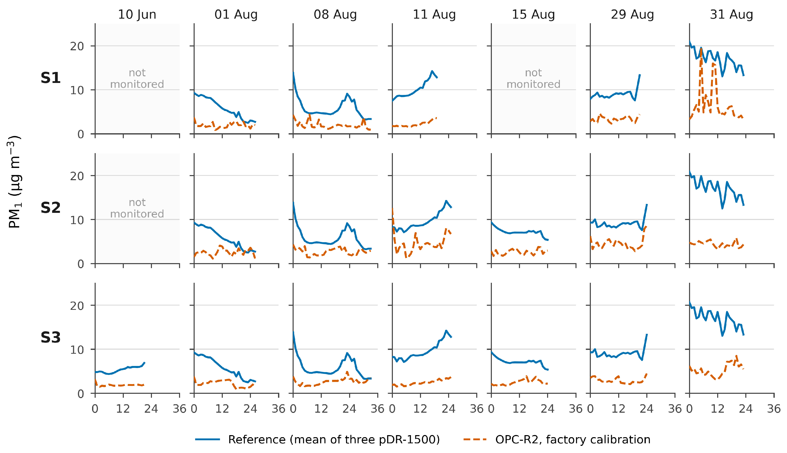
Descriptive statistics for the cleaned hourly data are summarized in

Table 3. Descriptive statistics of cleaned hourly data. PM₁ in µg m⁻³, temperature in °C, RH in %.

Sensor	Sensor PM1 Mean/Median/SD	Reference PM1 Mean/Median/SD	Reference Range	Mean Bias	T Offset	RH Offset
S1	3.08/2.42/2.62	9.17/8.51/4.63	2.45–20.9	−6.09	+6.80	−22.7
S2	3.50/3.34/1.55	8.81/8.19/4.20	2.46–20.9	−5.31	+7.03	−23.1
S3	2.79/2.52/1.28	8.39/7.60/4.09	2.49–20.7	−5.60	+7.00	−22.5

, and the corresponding time series are presented in Figure 2. All three sensors substantially underreported PM₁ relative to the reference instrument. Mean sensor PM₁ concentrations were 3.08, 3.50, and 2.79 µg m⁻³ for S1, S2, and S3, respectively, whereas the corresponding reference means were 9.17, 8.81, and 8.39 µg m⁻³, yielding mean biases of −6.09, −5.31, and −5.60 µg m⁻³, respectively.

Sensor temperature exceeded the reference temperature by 6.80–7.03 °C, with an RH offset of −22.5 to −23.1 percentage points. This indicates that the sensors were likely subject to internal self-heating within their enclosures. Given that the factory conversion assumes a particle density of 1.65 g mL⁻¹ and a refractive index of 1.5 + i0 for PSL spheres, such a systematic offset is an expected outcome of applying these assumptions to ambient indoor aerosols of differing composition and morphology, as is well documented across the OPC class [22,25,34].

The temperature and humidity offsets were examined directly. Sensor dew point is displaced from reference dew point only −2.60 to −2.71 °C (SD 0.50–0.66; r = 0.929–0.971), whereas relative humidity is displaced by more than 22 percentage points. Predicting the sensor RH from the reference RH and the measured temperature offset at conserved absolute humidity leaves a residual of −5.28 to −5.52 percentage points. Internal self-heating therefore accounts for roughly 17 of the 23 percentage point RH depression, and the remaining ~5.5 points correspond to a bias in the sensor RH element equivalent to a −2.6 °C dew point offset. Because the heating is a property of the enclosure rather than of the ambient air, a calibration trained on self-heated sensor RH is specific to that enclosure, which is a further reason to report the calibrated slope alongside R².

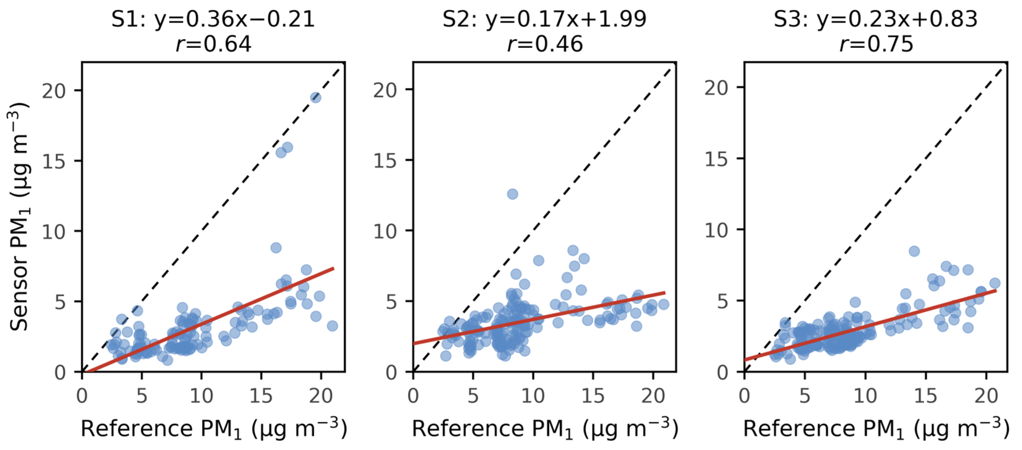
Goodness-of-fit statistics are summarized in

Table 4. Goodness-of-fit statistics of factory-calibrated sensor output and reference PM₁.

Sensor	Resolution	r	r2	Spearman’s Rho	R2	RMSE (µg m−3)	nRMSE (%)
S1	1-min	0.460	0.211	0.570	−1.490	7.59	82.3
	1-h	0.636	0.405	0.701	−1.341	7.06	77.0
S2	1-min	0.402	0.162	0.468	−1.369	6.70	75.8
	1-h	0.464	0.216	0.602	−1.407	6.49	73.6
S3	1-min	0.581	0.338	0.485	−1.498	6.68	78.9
	1-h	0.751	0.564	0.598	−1.516	6.47	77.0

, and the corresponding scatter plots are presented in Figure 3. Pearson correlation coefficients were 0.460, 0.402, and 0.581 at 1-min resolution, increasing to 0.636, 0.464, and 0.751 at hourly resolution. Values of r² ranging between 0.162 and 0.564 coexisted with R² values ranging from −1.341 to −1.516. RMSE values were 6.47–7.59 µg m⁻³ (74–82% of the mean). Figure 3 also shows regression slopes of 0.16–0.36, so that the sensors compress the reference dynamic range by roughly a factor of three to six before correction.

3.2. Calibration Under Random Hold-Out

Under the random 80%/20% split (

Table 5. Calibration performance under random 80/20 hold-out (mean. ± standard deviation) over three seeds.

		S1		S2		S3
Res.	Model	R2	RMSE (nRMSE %)	R2	RMSE (nRMSE %)	R2	RMSE (nRMSE %)
1-min	MLR	0.474 ± 0.000	3.40 (37)	0.545 ± 0.000	2.92 (33)	0.599 ± 0.000	2.68 (32)
	SVR	0.779 ± 0.001	2.21 (24)	0.769 ± 0.015	2.08 (24)	0.738 ± 0.000	2.16 (26)
	RF	0.886 ± 0.001	1.58 (17)	0.879 ± 0.008	1.51 (17)	0.878 ± 0.001	1.48 (17)
	GBR	0.863 ± 0.009	1.73 (19)	0.858 ± 0.005	1.63 (18)	0.855 ± 0.012	1.61 (19)
	XGB	0.861 ± 0.003	1.75 (19)	0.852 ± 0.006	1.67 (19)	0.857 ± 0.010	1.60 (19)
	LGBM	0.875 ± 0.003	1.66 (18)	0.878 ± 0.002	1.52 (17)	0.859 ± 0.003	1.59 (19)
1-h	MLR	0.428 ± 0.000	2.97 (32)	0.430 ± 0.000	2.94 (33)	0.726 ± 0.000	2.50 (30)
	SVR	0.818 ± 0.000	1.68 (18)	0.732 ± 0.021	2.02 (23)	0.810 ± 0.000	2.09 (25)
	RF	0.811 ± 0.017	1.71 (19)	0.593 ± 0.150	2.48 (28)	0.855 ± 0.005	1.82 (22)
	GBR	0.886 ± 0.006	1.32 (14)	0.664 ± 0.017	2.26 (26)	0.867 ± 0.002	1.75 (21)
	XGB	0.821 ± 0.035	1.66 (18)	0.696 ± 0.007	2.15 (24)	0.856 ± 0.006	1.82 (22)
	LGBM	0.689 ± 0.005	2.19 (24)	0.668 ± 0.009	2.24 (25)	0.836 ± 0.012	1.94 (23)

Note: Bold indicates the best-performing model for each sensor and temporal resolution.

) at 1-min resolution, Random Forest achieved R² values of 0.886, 0.879, and 0.878 for S1, S2, and S3, respectively, with RMSE ranging from 1.48 to 1.58 µg m⁻³ (17% of the mean). LightGBM (R² = 0.859–0.878) and other boosting models (0.852–0.863) followed closely, whereas SVR achieved R² values of 0.738–0.779 and MLR trailed at 0.474–0.599. At hourly resolution, the top-performing models were GBR for S1 (R² = 0.886) and S3 (R² = 0.867), and SVR for S2 (R² = 0.732).

3.3. Calibration Under Blocked and Prospective Validation Designs

Under day-blocked cross-validation (

Table 6. Calibration performance under day-blocked five-fold cross-validation (mean ± standard deviation) over three seeds.

		S1		S2		S3
Res.	Model	R2	RMSE (nRMSE %)	R2	RMSE (nRMSE %)	R2	RMSE (nRMSE %)
1-min	MLR	−0.194 ± 0.000	5.26 (57)	−0.055 ± 0.000	4.47 (51)	0.447 ± 0.000	3.14 (37)
	SVR	0.039 ± 0.071	4.71 (51)	0.190 ± 0.065	3.91 (44)	0.457 ± 0.016	3.11 (37)
	RF	−0.146 ± 0.060	5.15 (56)	−0.344 ± 0.034	5.04 (57)	0.147 ± 0.028	3.90 (46)
	GBR	0.206 ± 0.016	4.29 (46)	−0.168 ± 0.041	4.70 (53)	0.152 ± 0.080	3.89 (46)
	XGB	0.147 ± 0.031	4.44 (48)	−0.191 ± 0.026	4.75 (54)	0.255 ± 0.076	3.64 (43)
	LGBM	−0.074 ± 0.072	4.99 (54)	−0.408 ± 0.003	5.16 (58)	0.098 ± 0.007	4.01 (47)
1-h	MLR	0.033 ± 0.000	4.54 (50)	0.351 ± 0.000	3.37 (38)	0.590 ± 0.000	2.61 (31)
	SVR	0.318 ± 0.121	3.80 (41)	0.397 ± 0.059	3.24 (37)	0.249 ± 0.132	3.52 (42)
	RF	0.197 ± 0.097	4.13 (45)	0.053 ± 0.141	4.06 (46)	0.350 ± 0.022	3.29 (39)
	GBR	0.286 ± 0.070	3.89 (42)	0.081 ± 0.010	4.01 (45)	0.222 ± 0.019	3.59 (43)
	XGB	0.283 ± 0.042	3.91 (43)	0.075 ± 0.040	4.02 (46)	0.267 ± 0.048	3.49 (42)
	LGBM	0.115 ± 0.048	4.34 (47)	0.377 ± 0.005	3.30 (37)	0.145 ± 0.009	3.77 (45)

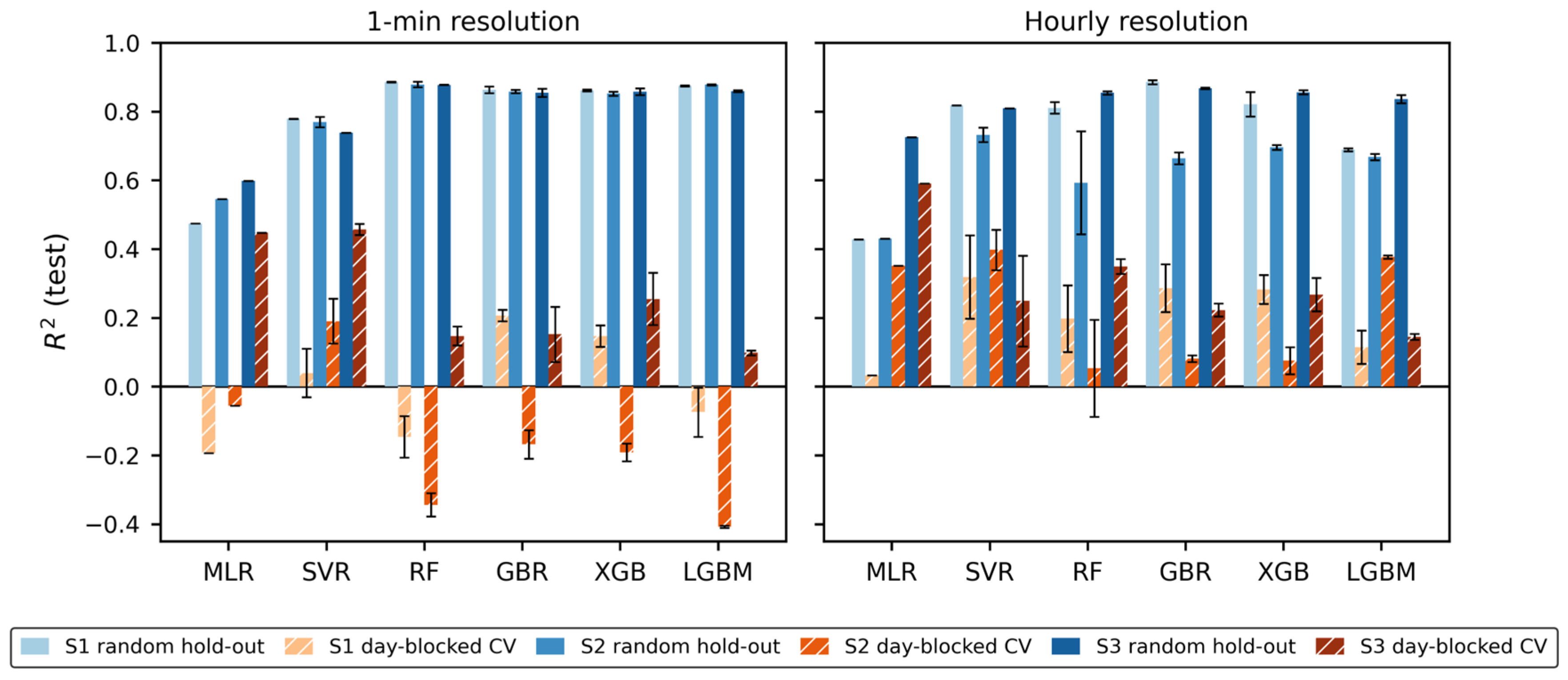
Note: Bold indicates the best-performing model for each sensor and temporal resolution.

), 1-min RF R² values dropped to −0.146 for S1, −0.344 for S2, and 0.147 for S3. LightGBM yielded the lowest performance, falling to −0.408 for S2. RMSE values escalated from approximately 1.5 µg m⁻³ to 3.9–5.2 µg m⁻³ (44–58% of the mean). Bar charts comparing model performance under random hold-out and day-blocked cross-validation across all three sensors and two temporal resolutions are presented in Figure 4.

Under random splitting, a decision tree ensemble performed well in five of the six sensor resolution combinations, whereas MLR performed the worst across all six. Under day-blocked validation, SVR yielded the highest accuracy in four combinations, and GBR and MLR in one each; conversely, random forest failed to achieve top performance in any scenario and ranked as the worst or second-worst model in four out of six cases. The highest single R² value under day-blocked validation was achieved by MLR (R² = 0.590) for S3 at hourly resolution. At 1-min resolution for S2, all four decision tree ensembles generated negative R² values despite hyperparameter optimization and seed iterations. LightGBM, with an R² of −0.408, performed substantially worse than simply reporting the campaign mean for every observation.

MLR is deterministic, yielding zero standard deviation throughout. Conversely, ML models return standard deviations up to 0.150 (RF for S2 at hourly resolution under random splitting) and 0.141 (RF for S2 at hourly resolution under day blocking); this implies that a single-seed result for the given configuration could have been reported anywhere roughly between 0.44 and 0.74. At hourly resolution, the lowest day-blocked RMSE decreased from 7.06 to 3.80 µg m⁻³ (from 77% to 41% of the reference mean) for S1, from 6.49 to 3.24 µg m⁻³ (77% to 37%) for S2, and from 6.47 to 2.61 µg m⁻³ (77% to 31%) for S3—representing relative reductions of 46.2%, 50.1%, and 59.7%, respectively.

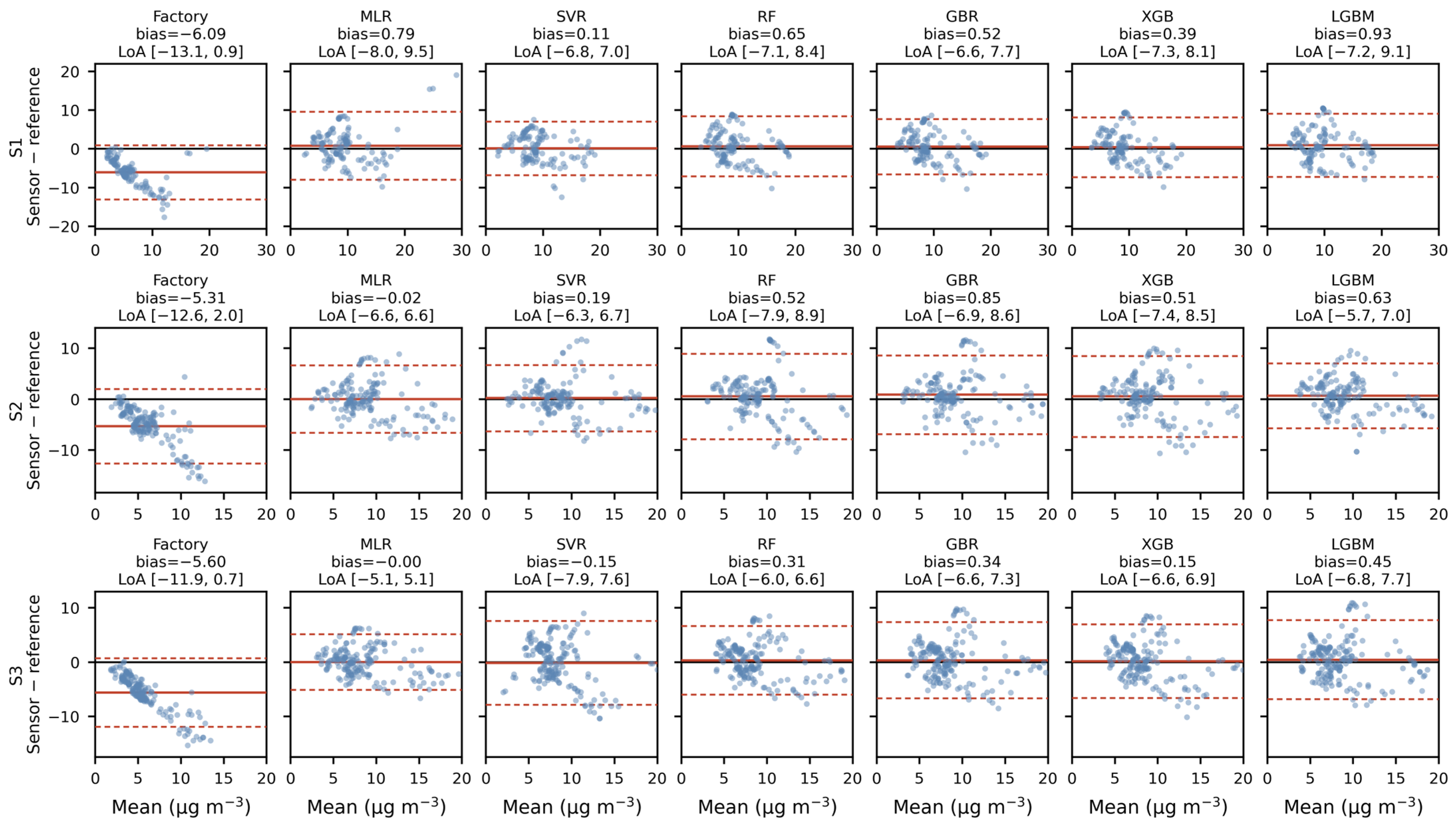
Figure 5 shows the corresponding Bland–Altman plots for each model. The factory-calibrated output exhibits a pronounced proportional error, with the bias remaining near zero at low concentrations and expanding below −15 µg m⁻³ at the upper end of the range; this explains why a single scaling factor cannot correct it. All calibrated models almost completely eliminate the mean bias (−0.15 to +0.93 μg m⁻³); however, the limits of agreement remain broad, ranging from [−5.1, +5.1] μg m⁻³ for MLR on S3 to [−8.0, +9.5] μg m⁻³ for MLR on S1. Consequently, calibration corrects the systematic offset without substantially reducing the uncertainty of an individual measurement.

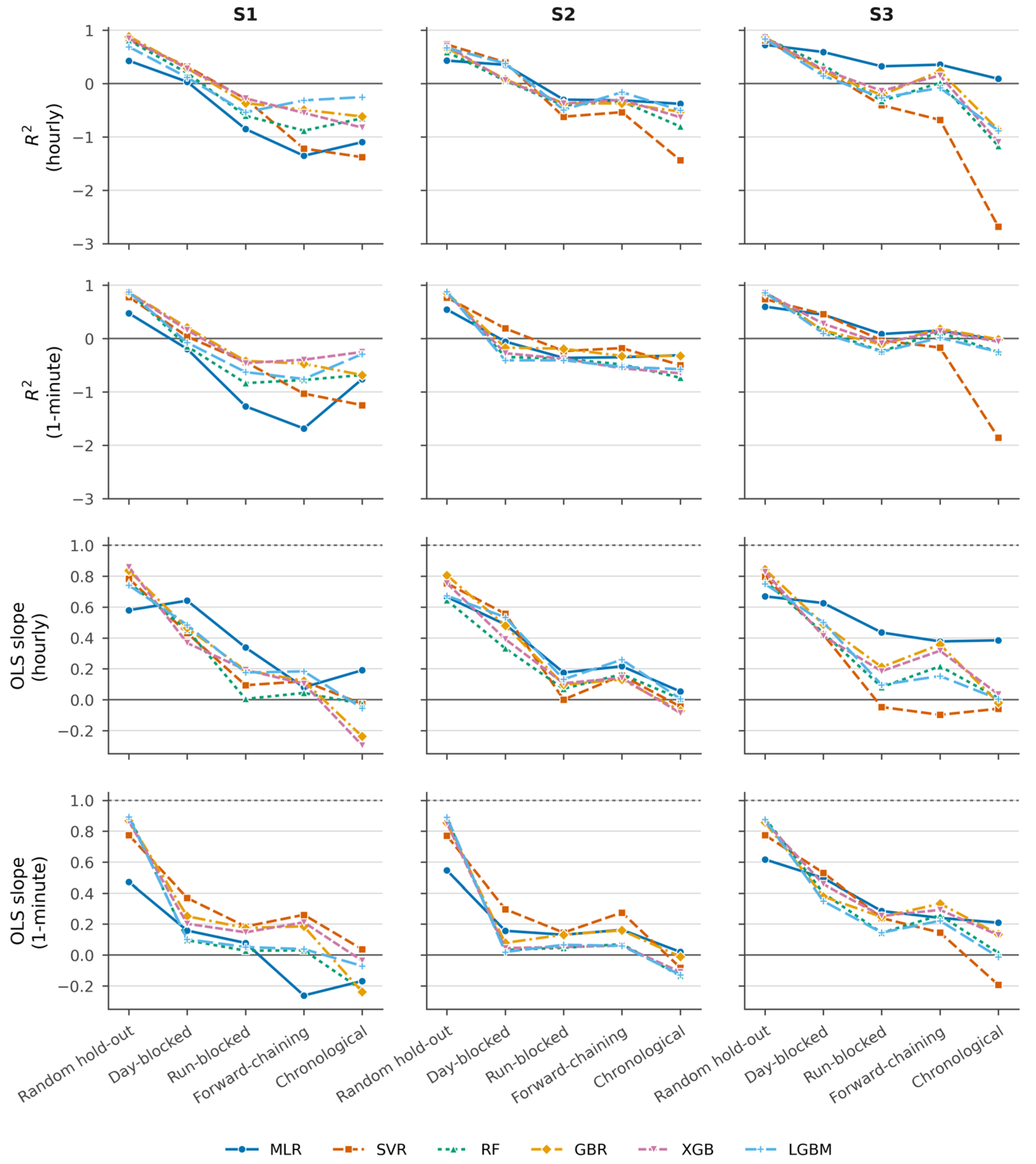
Extending the comparison to leave-one-run-out cross-validation, forward chaining and a chronological hold-out (Figure 6) shows that R² fell sharply from random to day-blocked to run-blocked validation, and remained near or below zero under forward chaining and the chronological hold-out. Averaged over the six models, R² falls from 0.74, 0.64 and 0.83 under random splitting to 0.21, 0.19 and 0.37 under day-blocked cross-validation and to −0.49, −0.43 and −0.16 under leave-one-run-out cross-validation for S1, S2 and S3. The best RMSE per design rises from 1.25–2.04 µg m⁻³ under random splitting to 2.61–3.80 µg m⁻³ under day blocking and 3.35–5.22 µg m⁻³ under run blocking, against a factory baseline of 6.47–7.06 µg m⁻³. Calibration therefore remains beneficial under every design, but the benefit is a 22–48% reduction in RMSE prospectively rather than the 46–60% obtained under day blocking.

The calibrated regression slope is the more revealing quantity. For the best model under each design, the slope falls from 0.75–0.84 under random splitting to 0.43–0.63 under day blocking and 0.18–0.44 under run blocking and forward chaining. A model that reproduces the mean concentration but compresses its variation by 56–82% corrects the systematic offset without recovering the signal, which is consistent with the broad limits of agreement reported above.

Decomposing the spread in R² across the five designs and six models attributes 81.1%, 91.1% and 62.7% of it to validation design for S1, S2 and S3 (at 1-min resolution), against 10.6%, 3.6% and 7.8% to the choice of algorithm. Pooling the three sensors gives 71.3% against 3.7% at 1-h resolution and 66.7% against 2.0% at 1-min resolution. The ranking of models is not merely displaced but decoupled: averaged over the 12 sensor × blocked-design combinations, the Spearman correlation between the model ranking under random splitting and that under each blocked design was 0.00 at hourly and −0.28 at 1-min resolution, with individual values between −0.89 and +0.94.

3.4. Feature Importance Under Temporal Validation

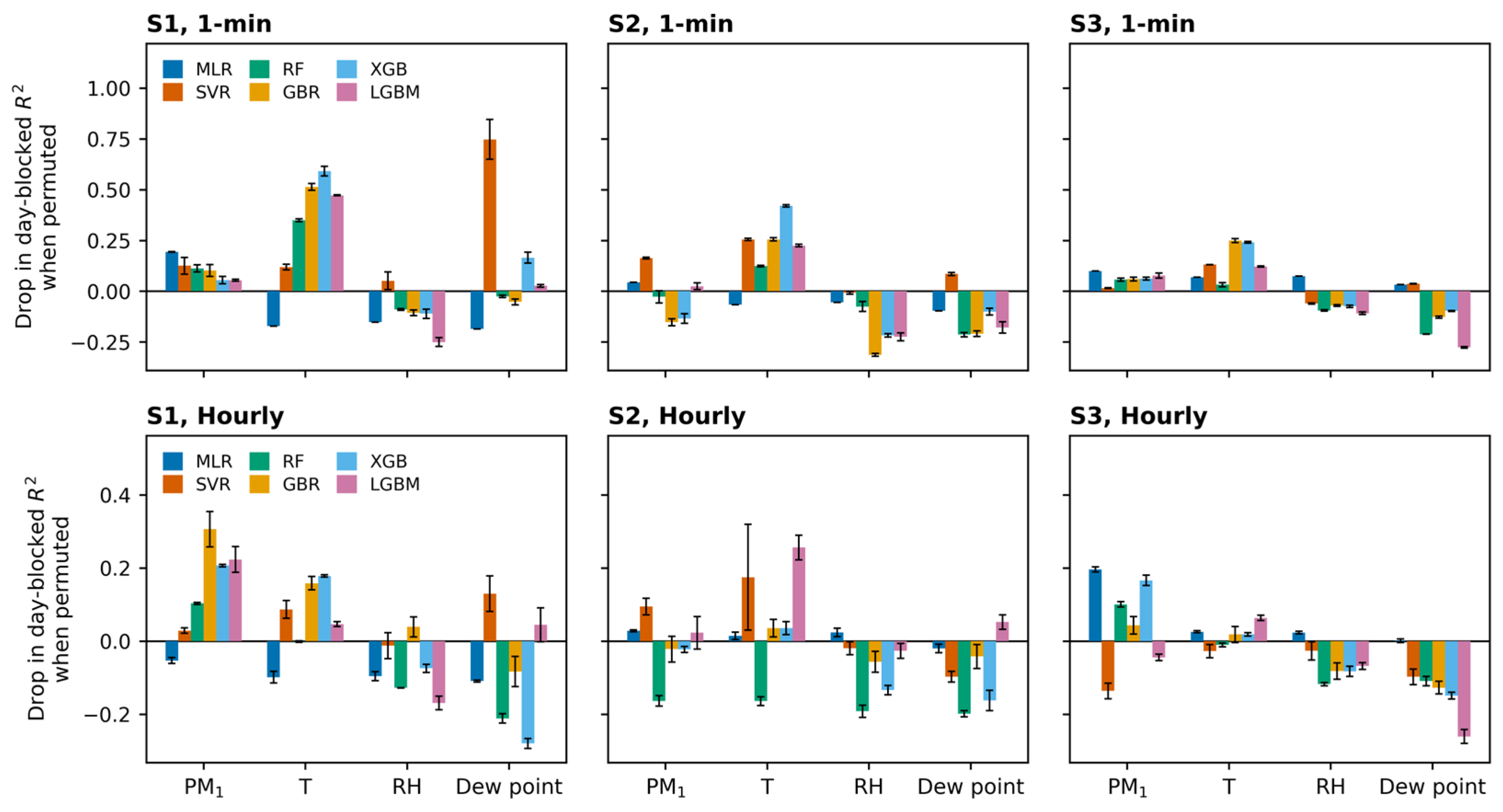
Permutation feature importance measured on day-blocked, out-of-fold predictions is presented in Figure 7. Out of 144 model–sensor–predictor–resolution combinations, 73 yielded negative values: randomizing a predictor frequently improved the out-of-fold R² score. Negative values were most prevalent in RF (occurring in 71% of its combinations) and least frequent in SVR (38%), aligning with the model capacity ranking observed in Table 6. For the hourly RF model on S2, all four predictors produced negative importance values ranging between −0.164 and −0.199.

Two predictors exhibited consistent behavior. The sensor’s native PM₁ channel proved to be the most reliably useful variable, yielding positive importance values in 27 of 36 combinations. Sensor temperature was likewise predominantly positive, emerging as the single most important predictor for decision tree ensembles at 1-min resolution, where it reached values of 0.514 for GBR and 0.592 for XGB on S1. Dew point behaved in the opposite manner. It was negative in most combinations and proved to be the most detrimental predictor for RF across all three sensors (ranging from −0.109 to −0.214); conversely, permuting dew point for S1 under SVR at 1-min resolution induced an R² loss of 0.748, representing the largest single impact observed in this study. Sensor RH yielded negative values in the majority of cases.

Because dew point is a deterministic function of temperature and RH, these single predictor values are not a reliable guide, and the analysis was repeated for all three sensors with the three meteorological variables permuted as one block under leave-one-run-out validation at 1-min and hourly resolution (hourly values in brackets). When the block was permuted throughout and the model refitted, permuting the meteorological block raised out-of-run R² in 15 of the 18 sensor–model combinations at both resolutions by up to 1.228 [0.963]. Permuting the sensor PM₁ channel lowered R² in 15 [16] of 18, by up to 1.066 [0.707]. When each model was fitted once and the block permuted only in the held-out fold, the meteorological block produced small drops (up to 0.090 [0.119]), and the PM₁ channel changed R² by less than 0.031 [0.092]. The two definitions therefore diverge on the meteorological block: fitted models use temperature, humidity and dew point when predicting a new run, yet models trained without them predict held-out runs better. This indicates that the structure learned from the meteorological variables does not transfer between runs. Hourly aggregation changes the magnitudes and which few combinations are exceptions, but not this conclusion. Because out-of-run R² was already negative in 17 of 18 combinations at both resolutions and permuting a predictor can then raise R² mechanically by pulling predictions toward the mean, negative importance is a symptom consistent with non-transferable structure rather than direct evidence of it.

3.5. Sensitivity to Temporal Aggregation and Predictor Set

Table 7. Day-blocked R² by predictor set. “4-var” = PM₁, T, RH, dew point; “6-var” adds sensor PM_2.5 and PM₁₀.

Res.	Model	S1 4-var	S1 6-var	S2 4-var	S2 6-var	S3 4-var	S3 6-var
1-min	MLR	−0.194	−0.193	−0.055	−0.049	0.447	0.459
	SVR	0.039	0.040	0.190	0.131	0.457	0.445
	RF	−0.146	−0.124	−0.344	−0.363	0.147	0.135
	GBR	0.206	0.168	−0.168	−0.152	0.152	0.170
	XGB	0.147	0.002	−0.191	−0.197	0.255	0.286
	LGBM	−0.074	−0.076	−0.408	−0.395	0.098	0.053
1-h	MLR	0.033	−0.048	0.351	0.200	0.590	0.593
	SVR	0.318	0.141	0.397	0.387	0.249	0.190
	RF	0.197	0.155	0.053	0.088	0.350	0.345
	GBR	0.286	0.216	0.081	0.015	0.222	0.247
	XGB	0.283	0.179	0.075	0.077	0.267	0.268
	LGBM	0.115	−0.001	0.377	0.334	0.145	0.207

reports the comparison of predictor sets. Across all 36 combinations, the four-predictor set outperformed the six-predictor set in 21 instances, yielding a higher mean day-blocked R² value of 0.137 compared to 0.109. This advantage was concentrated at hourly resolution (12 out of 18 instances, 0.244 versus 0.200), whereas the two sets were nearly indistinguishable at 1-min resolution (9 out of 18 instances, 0.031 versus 0.019). For S2, SVR—which yielded the highest performance among the four-predictor models at both hourly and 1-min resolutions—produced lower R² values across all six-predictor configurations. Conversely, for S3, MLR—which achieved the best performance at both resolutions—demonstrated higher R² values when using the four-predictor set compared to the same model specified with six predictors. Combined with the multi-collinearity diagnostics in Section 2.5, these findings support a parsimonious specification.

Four predictor sets were compared under leave-one-run-out validation: sensor PM₁ alone, PM₁ with temperature and relative humidity, the four-variable set that adds dew point, and the six-variable set that adds the cumulative size fractions. PM₁ alone gave the highest out-of-run R² in 27 of the 36 sensor × resolution × model combinations, PM₁ + T + RH in 8 and the six-variable set in 1. Averaged over the six models at hourly resolution, out-of-run R² was −0.08, −0.14 and +0.13 for PM₁ alone (S1, S2, S3), −0.32, −0.29 and −0.11 for PM₁ + T + RH, −0.51, −0.44 and −0.16 for the four-variable set and −0.66, −0.55 and −0.21 for the six-variable set; the mean therefore fell monotonically as predictors were added. At 1-min resolution the ordering was less regular, but PM₁ alone remained the best set in most combinations.

The sensitivity of these results to the two data-cleaning filters was tested by repeating the random, day-blocked and leave-one-run-out designs for all six models under four filter configurations, with each filter applied or omitted. The humidity filter removed 67, 92 and 93 one-minute records for S1, S2 and S3, all on 29 and 31 August, at reference PM₁ of 15.4–18.2 µg m⁻³; the outlier filter removed 107, 48 and 129 records whose reference PM₁ (8.7–9.2 µg m⁻³) matched the retained data but whose sensor readings reached 51–3877 µg m⁻³. Removing either filter changed the magnitudes but not the ordering of the designs: across all 144 sensor × resolution × filter × model combinations, R² was higher under random splitting than under day blocking, and higher under day blocking than under leave-one-run-out validation in 141 of 144. Averaged over the six models, the gap between random and run-blocked validation remained 1.00–1.50 in R² at hourly and 0.90–1.53 at 1-min resolution, and the run-blocked mean was negative in all 24 configurations. The outlier filter was the more influential of the two: omitting it lowered the hourly run-blocked mean from −0.49 to −0.77 for S1, from −0.43 to −0.47 for S2 and from −0.17 to −0.30 for S3, whereas omitting the humidity filter changed the hourly means by less than 0.07 in either direction.

4. Discussion

4.1. Comparison with the Literature

Cross-validation is inherently designed to evaluate overfitting by estimating model performance on unseen data from the same distribution. While random K-fold splitting is appropriate for diagnosing whether complex models have overfitted to their training samples, it fails to address the primary concern of prospective sensor users: predicting post-calibration performance. Over time, variables such as temperature, humidity, aerosol composition, occupancy, and sensor aging inevitably alter operating conditions. This introduces a domain shift—a change in the underlying data distribution, not merely a further sample from it.

Goodarzi et al. [53] make the distinction explicit for industrial condition monitoring: across seven datasets, random K-fold validation returned near-perfect accuracy for every model tested, whereas leave-one-group-out validation across deliberately varied operating conditions produced substantially lower and more dispersed accuracies, and low-capacity classical pipelines outperformed deep networks in four of the seven cases. The results reported here reproduce that pattern for low-cost PM₁ calibration, and the two questions should be reported separately rather than conflated in a single coefficient of determination.

Our random-split results at 1-min resolution (R² = 0.86–0.89, RMSE at 17% of the mean) lie within the upper range reported for the ML calibration of low-cost PM sensors, alongside the values of Wang et al. [36] (R² up to 0.99), Taştan [33] (0.970), and Srisang et al. [54]. Conversely, our day-blocked results at hourly resolution (best R² = 0.318–0.590) align closely with those reported by Villarreal-Marines et al. [25] from a year-long deployment (R² ~ 0.5 following XGBoost calibration), and exceed those of Attey-Yeboah et al. [26] (0.18–0.27). Both studies, deployed over extended periods and subject to seasonal variation, report values close to our out-of-time estimates, whereas studies evaluated strictly within the co-location period report performance metrics close to our random-split estimates. Koziel et al. [22] addressed this issue from a different perspective by explicitly aligning sensor and reference time series, while Espezúa et al. [55] found temporal features to be critically important—both findings being consistent with temporal structure serving as a primary determinant of apparent calibration quality. None of this implies that sensors evaluated in the literature perform poorly; rather, it indicates that reported metrics frequently describe interpolation within the co-location campaign itself, rather than the quantity needed by a prospective user—namely, predictive performance during a subsequent deployment following co-location.

Most of the calibration studies compared above were conducted outdoors, where co-location campaigns lasting several months to a year cover wide concentration and humidity ranges, and relative humidity is often the most influential covariate [34]. Indoor campaigns are typically shorter, and concentrations are driven by episodic, source-related peaks rather than gradual seasonal variation [14,33]. With less independent variance to explain, indoor R² is more easily inflated by concentration levels shared within a session, and more easily turns negative once whole sessions are withheld. Consequently, indoor calibration results are more sensitive to the validation design than those obtained outdoors, which the transfer tests discussed below illustrate. Taken together, transfer tests between weeks and stations [22], between outdoor sites [56] and between indoor microenvironments [14] show that skill can be lost once the evaluation leaves the training context; the present indoor results reproduce this loss in a more pronounced form.

The most directly comparable evidence stems from studies that evaluated their calibrations twice: once under the conditions in which the model was trained, and once following a change in environmental context. Nowack et al. [56] calibrated low-cost NO₂ and PM₁₀ sensors against reference stations in London and subsequently transferred the calibrated devices between sites. For PM₁₀, they obtained an R² of approximately 0.79 using ridge regression and Gaussian process regression at the co-located site; however, when models trained at one site were applied to another, this value dropped to between 0.37 and 0.53, with the extent of performance loss depending on the direction of transfer. Chojer et al. [14] conducted a similar test across microenvironments within a single school building: a calibration developed in one classroom transferred acceptably to a second classroom (RMSE: 7.19 µg m⁻³), whereas when applied to the cafeteria, it failed via severe overestimation—despite an apparently high R² of 0.89 (RMSE: 34.89 µg m⁻³, mean bias +31.59 µg m⁻³).

At 1-min resolution, indoor PM₁ concentrations evolve slowly relative to the sampling interval; consequently, consecutive records are nearly identical. A random 80%/20% split places an average of four out of every five records within any short time window into the training set, leaving the fifth record surrounded by near-duplicates of itself. A sufficiently flexible learner can thus achieve low error not by learning and modeling the sensor’s optical response, but by locating each test observation within the training manifold. Hourly aggregation mitigates this redundancy but does not eliminate it: within runs, the autocorrelation of the reference series is 0.93–0.94 at a lag of 1-min and still 0.62–0.67 at 60 min. Zhu et al. [39] classify this condition as data leakage arising from time-dependent data splitting and prescribe block splitting as the remedy. This mechanism accounts for the performance reversal across validation schemes. MLR, possessing very few parameters, cannot exploit local temporal redundancy; hence, its performance changes relatively little between designs (hourly S3: 0.726 → 0.590), whereas RF loses most of its apparent skill (1-min S2: 0.879 → −0.344). SVR is competitive under random splitting (mean R² = 0.786), but is the weakest model in seven of the nine sensor × prospective design combinations, falling to −2.68 under the chronological hold-out for S3.

A second mechanism, which dominates here, operates at the scale of whole runs. Run-mean reference concentrations range from 5.3 to 17.0 µg m⁻³, whereas the within-run standard deviation is only 0.6–3.6 µg m⁻³. The within-run hourly sensor–reference correlation is weak and inconsistent (−0.19 to 0.95, mostly 0.1–0.5), against a pooled correlation of 0.46–0.75. Apparent agreement therefore reflects the sensor and the reference registering the same run-level concentration rather than tracking variation within a run. Any design that leaves part of a test run in training can recover that run’s level. Holding the whole run out forces extrapolation to an unseen level, and the calibrated slope collapses accordingly.

4.2. Practical Recommendations

For studies calibrating low-cost PM sensors against reference instruments, we recommend reporting out-of-time validation as the primary outcome, and grouping by measurement session rather than by calendar date: where a campaign consists of discrete co-location runs, a run that straddles midnight will otherwise be split across partitions. Forward chaining over chronologically ordered sessions, with a gap between the training and test periods, should be preferred where the number of sessions allows it, with leave-one-session-out cross validation as the alternative. Random-split results may be reported alongside but should be labeled as intra-campaign interpolation. Because the seed-to-seed dispersion we observed reached 0.15 in R², results should be repeated across multiple random seeds. Meteorological variables measured by the reference instrument should be excluded from the predictor set unless the target deployment scenario actually provides them, and predictor suites should be checked for redundancy. Cumulative size fractions derived from optical histograms convey substantially overlapping information. Permutation importance evaluated under an out-of-time design serves as a useful diagnostic. Negative importance values are consistent with a model having a non-transferable structure, although they are not direct evidence of it. Since permuting a predictor can raise an already negative R² mechanically, predictors that are deterministically related should be permuted as a block. Finally, the calibrated regression slope should always be reported, because R² and RMSE can both look acceptable while the calibrated output compresses real variation severely.

4.3. Limitations

The campaign comprised five to seven discrete co-location runs within a single laboratory, deliberately scheduled on days without laboratory activity and therefore characterized by a relatively narrow concentration range (hourly reference PM₁ 2.5–21.0 µg m⁻³, mean 8.4–9.2 µg m⁻³), which restricts extrapolation to higher-concentration or more dynamic environments; furthermore, low absolute concentrations imply that a given nRMSE corresponds to a small absolute error. Only three units of a single OPC model were evaluated, and their deployment periods were not identical. The sensors were read through a custom microcontroller-based acquisition system rather than the manufacturer’s single-sensor software, and no side-by-side comparison between the two configurations was performed. Because the system retrieves the sensor’s own output over SPI using the manufacturer-provided control code, it is not expected to alter the reported concentrations. However, possible effects of the regulated power supply, the 10 s polling with subsequent 1-min averaging, and the enclosure, which contributes to the self-heating described in Section 3.1, cannot be separated from the sensor response. The data acquisition interruptions that removed 12.3% of the S1 records are likewise specific to this system. Consequently, our results should be interpreted as characterizing these specific sensors under these particular conditions, rather than benchmarking the entire product line. Reference instruments were photometric monitors rather than gravimetric samplers, so the reported agreement is relative to a photometric transfer standard. Hyperparameter grids were intentionally kept compact; while a more exhaustive search or metaheuristic optimization might shift absolute performance, it would not alter the comparative findings between validation designs, as both relied on identical search procedures. The choice of predictor set described in Section 2.5 was informed by diagnostics computed over the complete dataset rather than strictly within training folds—representing a departure from rigid leakage isolation. The impact is likely minor given that this decision rested primarily on the physical redundancy of cumulative size fractions, yet it is acknowledged for transparency. Finally, hourly analyses rely on 127–183 observations and, as noted in Section 2.4, are utilized for interpretation and literature comparison rather than model selection.

A further limitation applies to the prospective designs themselves. Leave-one-run-out cross-validation and forward chaining test transfer only between sessions within one laboratory and, with the exception of the June run for S3, within a single season. They therefore remain optimistic relative to true deployment, which would additionally involve changes of site, aerosol regime and season. The estimates reported here should be read as an upper bound on prospective performance, and, correspondingly, the leakage effect demonstrated is a conservative lower bound. Cross-site and seasonal validation remain necessary future work.

5. Conclusions

Factory-calibrated PM₁ outputs from three Alphasense OPC-R2 sensors systematically underestimated co-located reference nephelometers (mean bias −5.3 to −6.1 µg m⁻³; regression slopes 0.16–0.36), yielding RMSE values of 6.5–7.6 µg m⁻³, which correspond to 74–82% of the reference mean (8.4–9.2 µg m⁻³). The sensors nevertheless tracked the temporal pattern of the reference instrument (hourly r = 0.46–0.75), demonstrating that field calibration is both necessary and effective: under prospective validation in which whole measurement sessions were held out, RMSE was reduced 22–48%. However, the magnitude of this improvement depends decisively on how it is measured. Identical data and models yielded R² values of 0.86–0.89 under a conventional random 80%/20% split, and progressively lower values under day-blocked, leave-one-run-out, forward-chaining and chronological designs. Validation design accounts for 63–91% of the spread in R² and algorithm choice accounts for 3.6–10.6%.

Gradient-boosted decision trees and random forests dominated under random splitting and several of them underperformed compared to a mean baseline once temporal leakage was removed. The ranking did not simply invert, however: it decoupled, so that a ranking obtained under random splitting carries essentially no information about the ranking under a prospective design. Multiple linear regression, the worst model under random splitting on every sensor, was the best model in half of the sensor x blocked-design combinations at hourly resolution (two of 12 at 1-min resolution). Permutation analysis was consistent with the diagnosis: randomizing predictors frequently improved out-of-fold performance, most often for the models that lost the most skill, and permuting the meteorological block improved out-of-run R² in 15 of 18 sensor-model combinations at both resolutions.

We conclude that the performance metrics reported across much of the low-cost sensor calibration literature reflect the choice of validation design as much as they do sensor or algorithm quality. Adopting out-of-time validation—alongside reporting calibrated regression slopes, errors normalized to the reference mean, and random-seed iterations—is imperative for these metrics to reliably inform deployment decisions. Specifically, for the OPC-R2 under the co-location conditions examined here, hourly-averaged PM₁ calibrated with a parsimonious model corrects the systematic offset and is suitable for characterizing indoor concentration levels. It is not suitable for resolving spatial gradients: under leave-one-run-out and forward-chaining validation the calibrated slope falls to 0.18–0.44, so that real variation is compressed by 56–82%, against 35–53% under day-blocked validation. Demonstrating suitability for spatial work would require cross-site validation, which this campaign does not provide.