Article

Characteristics of Atmospheric CO2 at Shangri-La Regional Atmospheric Background Station in Southwestern China: Insights from Recent Observations (2019–2022)

1
Shangri-La Regional Atmospheric Background Station, China Meteorological Administration, Diqing 674400, China
2
Lijiang Meteorological Bureau, Lijiang 674199, China
3
Yunnan Climate Center, Kunming 650034, China
*
Authors to whom correspondence should be addressed.
Atmosphere 2026, 17(1), 3; https://doi.org/10.3390/atmos17010003
Submission received: 27 October 2025 / Revised: 12 December 2025 / Accepted: 16 December 2025 / Published: 19 December 2025
(This article belongs to the Section Atmospheric Techniques, Instruments, and Modeling)

Abstract

Southwestern China serves as a critical region for carbon sources and sinks, influenced by both natural ecosystems and anthropogenic activities. The Shangri-La atmospheric background station (28.01° N, 99.73° E), the only regional station in southwestern China, provides essential data for understanding CO2 dynamics. This study analyzes hourly CO2 mole fractions from 2019 to 2022. Background signals were extracted using the Robust Extraction of Baseline Signal (REBS) algorithm, and air-mass trajectories were analyzed using HYSPLIT model and Potential Source Contribution Function (PSCF) and Concentration Weighted Trajectory (CWT) methods. The REBS-derived background CO2 concentration increased from ~409 ppm in 2019 to ~417 ppm in 2022, yielding a growth rate of 1.9 ± 0.1 ppm yr−1, slightly lower than the 2010–2014 rate reported previously and consistent with the recent global slowdown associated with ENSO-driven carbon–climate variability. A coherent seasonal cycle, with spring maxima and late-summer minima, reflects the combined influence of biospheric uptake and monsoonal inflow. Comparison with the global marine boundary layer and Waliguan records shows similar phase and amplitude, confirming the representativeness of Shangri-La as a regional background site, albeit with a one-month phase lag to Waliguan station due to regional climatic and phenological differences. Trajectory and wind analyses identify southern Indo-Myanmar and Sichuan–Yunnan regions as major transport corridors influencing high-CO2 events. Overall, the results highlight that regional transport rather than local emissions dominates CO2 variability at Shangri-La. The derived background and transport signals thus provide an updated and internally consistent characterization of carbon-cycle variability over the southeastern Tibetan Plateau, offering critical observational support for future regional carbon budget assessments.

1. Introduction

Carbon dioxide (CO2) is the most important anthropogenic greenhouse gas (GHG), contributing more than 60% of the total radiative forcing from all long-lived GHGs [1,2]. Since the preindustrial period, global atmospheric CO2 concentrations have risen from approximately 280 ppm to over 420 ppm in 2024, mainly due to fossil fuel combustion, deforestation, and biomass burning [3,4]. This rapid increase has led to substantial climate warming, ocean acidification, and perturbations in the global carbon cycle.
Since the late 1950s, long-term in situ measurements of atmospheric CO2 concentration have been systematically conducted at many locations around the globe [5,6]. While anthropogenic emissions are largely concentrated in urban areas, where net fluxes per unit area greatly exceed those of natural ecosystems [7], background stations provide essential data on regional and hemispheric baselines, free from local pollution influences. Atmospheric background stations, typically located in remote, high-altitude, or coastal regions with minimal local anthropogenic influence, provide representative information on regional and global background concentrations of trace gases [8]. Classic examples include the Mauna Loa Observatory in Hawaii, which records the canonical “Keeling Curve” of rising CO2 [9], and Mt. Waliguan in Qinghai, China, a World Meteorological Organization/Global Atmosphere Watch (WMO/GAW) global station represents continental background air for East and Central Asia [10]. These continuous long-term records are the foundation for understanding both the secular increase in atmospheric CO2 and its seasonal variations linked to biospheric uptake and release, often termed the “breathing of the biosphere” [11,12].
Located at 28.01° N, 99.73° E (3554 m above sea level), the Shangri-La Atmospheric Background Station is the only regional station in southwestern China, situated on the southeastern edge of the Tibetan Plateau. Unlike urban-dominated regions such as the Pearl River Delta, which are heavily influenced by local anthropogenic emissions [13], Shangri-La is situated in a remote, high-altitude area surrounded by coniferous forests and mountain meadows, far from major cities and industrial centers. This setting ensures compliance with WMO standards for background monitoring, making it ideal for capturing representative atmospheric conditions of the Sichuan-Yunnan region and the plateau’s edge zone [14]. The site lies at the transition between the Asian monsoon and the westerlies, receiving air masses from both the Indian Ocean and the interior of the Asian continent. Earlier work by Fang et al. (2016) reported the first multi-year (2010–2014) observations of atmospheric CO2 and CO at Shangri-La, revealing a CO2 growth rate of 2.5 ± 1.0 ppm yr−1 and clear diurnal cycles influenced by local biospheric activity and transport contributions from Northern Africa and Southwestern Asia [15].
Although the Shangri-La station has been the subject of earlier observational studies [15], those analyses relied primarily on manual filtering procedures to derive seasonal cycles and trends, and applied trajectory/PSCF (Potential Source Contribution Function) diagnostics in a limited, representative-month framework for source attribution. More recently, a multi-site comparison that extended observations to 2010–2016 further updated trajectory-based source indications for the region [16], but still characterized transport mostly by seasonally representative months and with background selection approaches that retain subjective elements. These methodological choices limit the ability to (1) robustly separate slowly varying background CO2 from episodic transport or local biospheric signals, and (2) systematically evaluate event-scale CO2 signals. Observational and modelling studies have shown that ENSO and associated tropical–extratropical teleconnections modulate continental carbon fluxes and atmospheric transport pathways [17], while decadal changes in monsoon dynamics and Plateau–monsoon coupling can substantially alter boundary-layer development and lateral advection over the Tibetan Plateau margin [18,19,20].
Motivated by these gaps, the present study targets the 2019–2022 period and combines a robust, data-driven background extraction with systematic HYSPLIT-based 72 h back trajectories and source diagnostics. This integrated framework (1) objectively isolates background CO2 on hourly records across the full study period and derivates its annual growth rate, and (2) performs trajectory clustering and PSCF/CWT (Concentration Weighted Trajectory) analyses on the full trajectory ensemble (rather than on a few representative months) and identifies and interprets the potential source regions influencing high-CO2 concentrations through integrated trajectory. By doing so, we provide a timely methodological and observational update to earlier work and directly test whether there are new transport signatures at Shangri-La. It thus contributes to a more comprehensive understanding of carbon cycle dynamics across the Tibetan Plateau and the Asian monsoon domain, with implications for national carbon monitoring and global climate assessments.
The rest of this study is organized as follows. In Section 2, the basic information about the Shangri-La station is presented, including its geographical location and the measurement equipment employed at the site. In Section 3, the CO2 concentration measurement data at the Shangri-La station are presented, and some analyses are conducted to reveal the characteristics of its variations. Lastly, in Section 4, the conclusion of this study is drawn.

2. Materials and Methods

2.1. Sampling Site and Measurement System

The Shangri-La Atmospheric Background Station (28.01° N, 99.73° E; 3554 m above sea level)) is located in northwestern Yunnan Province on the southeastern margin of the Tibetan Plateau (Figure 1). The station is situated on a remote mountainside approximately 30 km north of Shangri-La City (population ~180,000), in a monsoon-dominated climate with an annual cumulative precipitation of ~630 mm and average temperature of 5.2 °C. The region experiences a distinct wet season (May–October) dominated by the Asian monsoon and a dry season (November–April) under the westerlies. The surrounding vegetation consists primarily of coniferous forests and mountain meadows. Air samples were collected from an intake at a 50 m high tower, positioned above the local vegetation canopy to ensure representative atmospheric mixing. Meteorological sensors (wind speed/direction, temperature, humidity, and pressure) were installed nearby to provide concurrent data for supporting analyses.
Continuous atmospheric CO2 measurements were conducted from 2019 to 2022 using a cavity ring-down spectrometer (G2401, Picarro, Inc., Santa Clara, CA, USA). This instrument has a manufacturer-stated precision of 50 and 20 ppb for CO2 in 5 s and 5 min. Ambient air was sampled from an inlet installed on a 50 m tower. The sampled air is drawn in by a vacuum pump through a dedicated sampling line and ultimately delivered to the analyzer at a stable flow rate of approximately 300 sccm (standard cubic centimeters per minute). Before analysis, the sample air was passed through a particulate filter and dried by a cryogenic trap (submerged in an ethanol bath maintained at approximately −60 °C) to minimize spectroscopic interference and dilution effects from water vapor. The total residence time from the inlet to the analyzer was kept below 60 s to ensure a rapid response and prevent sample alteration. An automated sampling module, equipped with a multi-position valve, was used to switch between ambient air, a high-concentration working standard gas (WH), and a target gas (T). WH and T were prepared and calibrated by the China Meteorological Administration, traceable to the WMO X2007 CO2 scale. The observed CO2 dry-air mole fractions were calibrated using coefficients of a linear fit based on the most recent standard gas (e.g., WH) measurement. The WH was measured every 4 h, and the T was measured every 4 h offset by 2 h to WH. Each gas measurement lasted for 5 min. Following each switch between gas sources, the first 3 min of data were discarded to allow for system stabilization; only the subsequent 2 min of stable data were used for calibration and analysis. Raw data, recorded at 5 s intervals, were aggregated into 5 min averages (actually 2 min average as mentioned above) and then calibrated, followed by hourly means. Data points affected by instrumental malfunctions, maintenance periods, or contamination events were flagged and excluded from the final dataset.

2.2. Data Processing and Analysis

2.2.1. Background Extraction

For filtering high temporal resolution CO2 data to quantify background levels and separate them from regional influences, the robust extraction of baseline signal (REBS) algorithm [21] was adopted, which has been widely applied in atmospheric monitoring due to its effectiveness in isolating baseline signals from short-term perturbations (e.g., [22,23,24]). Specifically, REBS performs iterative local regression with asymmetric residual weighting, preferentially fitting the lower envelope of the dataset while suppressing high-frequency anomalies from local respiration or short-term pollution. A 90-day moving window was used. Values within ± 2σ of the fitted baseline were designated as background, where σ denotes the standard deviation of the detrended residuals, while those above (>baseline + 2σ) and below (<baseline − 2σ) were labeled as pollution events and depletion events, respectively. In this study, the terms “pollution events” and “depletion events” are used to denote statistical anomalies relative to the REBS baseline. We clarify that these statistical labels do not strictly imply anthropogenic pollution or purely biological uptake, but rather indicate air masses with significantly enhanced or depleted CO2 levels relative to the regional background. The 90-day window follows the REBS configuration used in prior background studies, providing sufficient smoothing of seasonal structure while retaining synoptic variability. To ensure robustness, we performed sensitivity tests using window sizes of 60, 90, and 120 days. The calculated annual mean background concentrations differed by less than 0.3 ppm across these settings. Furthermore, we tested the impact of the standard deviation (σ) threshold. The 2σ threshold retained approximately 70% of the observations as background. Sensitivity tests indicated that a stricter threshold (e.g., 1.5σ) retained only ~60% of data, potentially excluding valid background signals, while a looser threshold (e.g., 2.5σ or 3σ) risked including more pollution/depletion events. Based on these tests, the selected parameters (90-day, 2σ) were deemed robust for isolating the regional background signal. In addition, annual baseline growth rates were derived by linear regression on background data.

2.2.2. Backward Trajectory Analysis

Air-mass transport pathways were evaluated using the Hybrid Single-Particle Lagrangian Integrated Trajectory (HYSPLIT) model version 5 [25], developed by National Oceanic and Atmospheric Administration (NOAA)’s Air Resources Laboratory (ARL). The model employs a Lagrangian approach, driven by meteorological fields, to determine the three-dimensional movement pathways of air parcels by integrating the equations of motion, thereby generating a set of trajectories arriving at the study location over a specified period. To categorize the trajectories into distinct transport pathway types, trajectories were grouped using an agglomerative hierarchical spatial clustering algorithm based on latitude and longitude. The procedure begins by treating each individual trajectory as its own cluster. At each iterative step, the algorithm evaluates all possible pairwise merges and selects the combination that results in the smallest increase in the total spatial variance (TSV). The TSV is defined as the sum of squared Euclidean distances between each trajectory’s endpoints and the corresponding mean endpoints of its assigned cluster. This merging process continues until all trajectories belong to a single cluster. The optimal number of clusters was determined by analyzing the rate of increase in TSV as clusters were merged. A sharp rise in this rate indicates the merging of dissimilar groups. Therefore, the cluster count immediately before the first significant surge in the variance growth rate was chosen as the final classification, ensuring cohesive and well-separated trajectory types.
Three-day (72 h) backward trajectories were computed every 6 h (e.g., 00, 06, 12, and 18 UTC for computational efficiency without losing generality) at 500 m above ground level using Global Data Assimilation System (GDAS) data at 1° × 1° resolution from NCEP (data available via: https://www.ready.noaa.gov/data/archives/gdas1/; accessed on: 10 September 2025). Cluster analysis, embedding in HYSPLIT based on trajectory distance and angle similarity, identified the dominant transport patterns. In this study, air masses traced within 0–200 km of the station were considered locally influenced, those within 200–1000 km as regionally transported, and those beyond 1000 km as long-range transport.
We acknowledge that the 1° × 1° resolution of the GDAS dataset may not fully resolve the complex terrain surrounding Shangri-La. To assess the robustness of the results, we performed a height-sensitivity test by initializing trajectories at 50 m, 100 m, 500 m, and 1000 m above ground level. Although minor variations exist, particularly within the immediate topographic basin of Shangri-La, the overall cluster patterns remain consistent across all initialization heights. This indicates that the major transport pathways identified in this study are relatively insensitive to initialization height and are thus robust at the synoptic scale. The choice of 500 m for the main analysis therefore represents a balanced compromise: it reduces the near-surface topographic uncertainties that are more pronounced at 50–100 m (commonly used in earlier studies [15,16]), while avoiding the excessive altitude represented by 1000 m.
Potential source regions were further examined using the Potential Source Contribution Function (PSCF) and Concentration Weighted Trajectory (CWT) methods [15,24,26,27]. The receptor domain (0°–70° N, 0°–120° E) was divided into 0.25° × 0.25° grid cells. The PSCF value is the probability of a trajectory appearing in the respective grid, representing the total retention time of all air masses in a certain grid divided by the total time. The PSCF for cell (i,j) were calculated as
P S C F i , j = m i , j n i , j   ,
where n i , j is the number of trajectory endpoints in the cell (i,j), and m i , j is the number associated with high-CO2 events. In the CWT method, each grid cell is assigned a weighted concentration by averaging the sample concentrations that have associated trajectories that crossed that grid cell. The CWT value C i j in the cell (i,j) is determined by using the following averaging formula:
C i j = 1 k = 1 N τ i j k k = 1 N C k τ i j k
where k is the index of the trajectory, N is the total number of trajectories, C k is the CO2 concentration at arrival of trajectory k , and τ i j k is the residence time of trajectory k in grid cell (i,j). Cells with higher CWT values correspond to stronger potential source contributions.

3. Results and Discussion

3.1. Temporal Distribution of Observed CO2

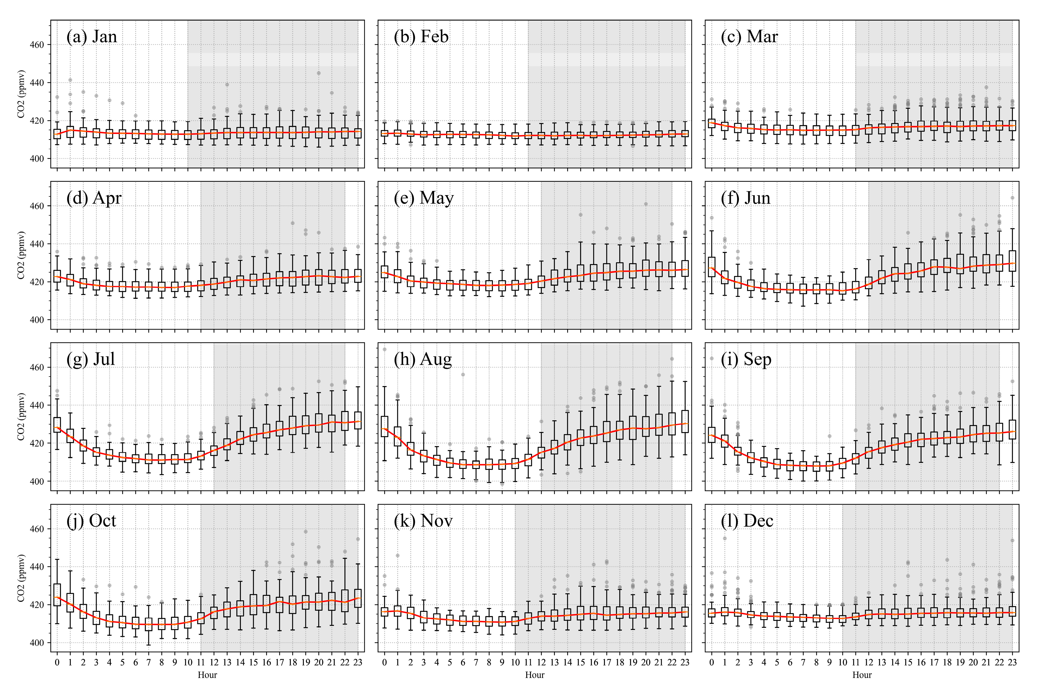
Figure 2 illustrates the composite monthly diurnal cycles of atmospheric CO2 observed at the Shangri-La station during 2019–2022 in UTC. It should be noted that the local time at the Shangri-La station is China Standard Time (CST), which is UTC + 8 h. Distinct seasonal patterns appear in both amplitude and phase. During the cold–dry season (November–April), hourly CO2 concentrations remain nearly constant throughout the day, reflecting weak biospheric activity and a persistently shallow boundary layer under stable stratification. In contrast, during the warm–wet season (May–October), diurnal amplitudes increase markedly, averaging 10.3 ± 6.2 (mean ± 1σ) ppm in spring (March-May), 25.0 ± 8.8 ppm in summer (June-August), 19.5 ± 8.4 ppm in autumn (September-November), and 5.8 ± 6.5 ppm in winter (December-February).
In a diurnal cycle, CO2 concentrations decline rapidly after sunrise (e.g., at 08:00 local time), reaching minima in the late afternoon (e.g., at 16:00 local time), followed by gradual nighttime accumulation. This pattern is commonly observed in ecosystems during the growing/wet season when daytime photosynthetic uptake and strong convective mixing dominate, while nocturnal stability enhances respiration-driven accumulation [28]. Moreover, the amplitude of the diurnal CO2 cycle is greater under active monsoon or wet-season conditions compared to dry seasons [29]. The intermediate amplitudes observed in April and October signify transitional meteorological conditions during the onset and withdrawal of the Asian monsoon [30]. The box-and-whisker distributions further demonstrate tight winter ranges (stable air, weak biogenic exchange) versus broad summer spreads (active vegetation and convective dynamics). The stronger diurnal amplitude in the warm season suggests a seasonal enhancement of surface biospheric activity and boundary-layer mixing, consistent with the characteristics of the regional monsoon period.

3.2. Filtered Background CO2 Observation

Figure 3 presents the hourly CO2 observations for 2019–2022, with the REBS baseline (solid green line) capturing the underlying background signal amid short-term fluctuations. Data gaps (e.g., in October 2021) resulted from instrument malfunction, gas system maintenance, or unexpected power interruptions. The background envelope was defined as the baseline ± 2σ. Observations exceeding the upper limit were classified as pollution events (red dots), representing episodic enhancements from local or regional CO2 inputs, whereas those below the lower limit were categorized as depletion events (blue dots), corresponding to net CO2 removal via vegetation uptake or atmospheric scavenging. The long-term trend line (sky-blue dashed line) was obtained by linear regression on the background signals, providing a robust estimate of secular evolution.
To evaluate the consistency between the raw CO2 series and the REBS-derived baseline, we quantified the seasonal cycle using the climatological monthly mean. The raw data show a seasonal amplitude of 10.21 ppm, while the REBS baseline shows 10.14 ppm, indicating negligible damping (~0.7%). The much larger hour-to-hour variability in the raw series (instantaneous excursions up to ~70 ppm) reflects short-term boundary-layer and synoptic effects. Approximately 70% of hourly observations fall within the baseline ±2σ envelope and are classified as background. These metrics confirm that the site predominantly samples regional background air while remaining sensitive to episodic perturbations. Annual mean background CO2 concentrations, derived from REBS-filtered data were 411.6 ppm (2019), 413.8 ppm (2020), 416.6 ppm (2021), and 418.5 ppm (2022). The background CO2 concentration increased steadily from approximately 409 ppm in early 2019 to 417 ppm by late 2022, corresponding to a long-term trend of 1.9 ± 0.1 ppm yr−1 (passing the Mann–Kendall test with p value < 0.05). This rate is slightly lower than the 2010–2014 period (2.5 ± 0.1 ppm yr−1) reported by Fang et al. (2016) [15], consistent with the temporary slowdown in global atmospheric CO2 growth [1], likely influenced by ENSO (El Niño-Southern Oscillation)-driven carbon-cycle variations [17,31,32].
In Figure 3, a coherent background seasonal cycle is evident throughout the study period, with maxima in April–May and minima in August–September. The seasonal peak occurs just before the monsoon onset, when wintertime CO2 accumulates under limited vertical mixing. The subsequent decline during summer reflects both enhanced photosynthetic carbon uptake and strong convective dilution by monsoon inflow from the Indian Ocean. Moreover, it highlights a distinct seasonal asymmetry in event distribution: pollution events concentrated between March and December while depletion events only concentrated between July and November. Given the station’s proximity to meadows and forests, depletion events are rationally attributed to intensified photosynthetic uptake by local vegetation, particularly during the growing season. As for pollution events, in addition to known local sources such as vegetation, backward trajectory analysis is essential to evaluate potential regional and long-range transport of pollutants.
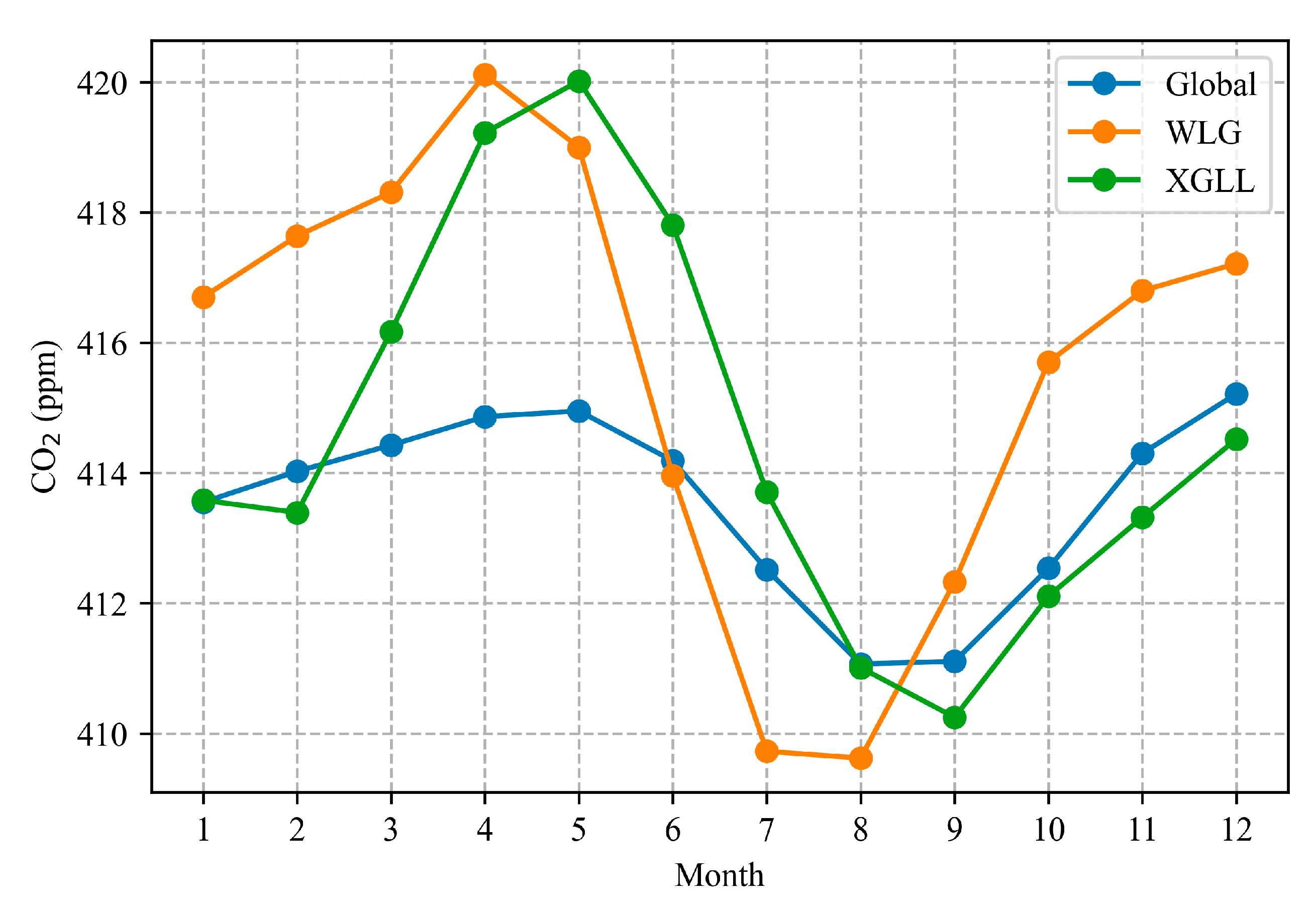
Compared with the earlier 2010–2014 record reported by Fang et al. (2016) [15], current observations show (1) higher mean background CO2, and (2) larger seasonal amplitude, both consistent with global post-2010 trends [1]. Figure 4 illustrates the seasonal cycle of regional CO2. For comparison, the data during the same period from Waliguan station (retrieved from https://gaw.kishou.go.jp/, accessed on 1 October 2025) are presented, as well as the global average surface CO2 from the Marine Boundary Layer (MBL) reference (retrieved from https://gml.noaa.gov/ccgg/mbl/data.php accessed on 1 October 2025). Overall, Shangri-La exhibits a temporal pattern closely aligned with both global and Waliguan station records. However, the phase of Shangri-La station’s seasonal cycle lags that of Waliguan station by approximately one month. Based on existing studies, later monsoon onset and distinct phenological timing at the southeastern plateau margin are plausible contributing factors [19,33,34]. The amplitudes of both stations are comparable, though Waliguan station shows higher background concentrations during autumn and winter. Relative to the global mean, surrounding region of Shangri-La behaves as a net CO2 source during spring and summer and as a net CO2 sink during autumn.

3.3. Trajectory Analysis

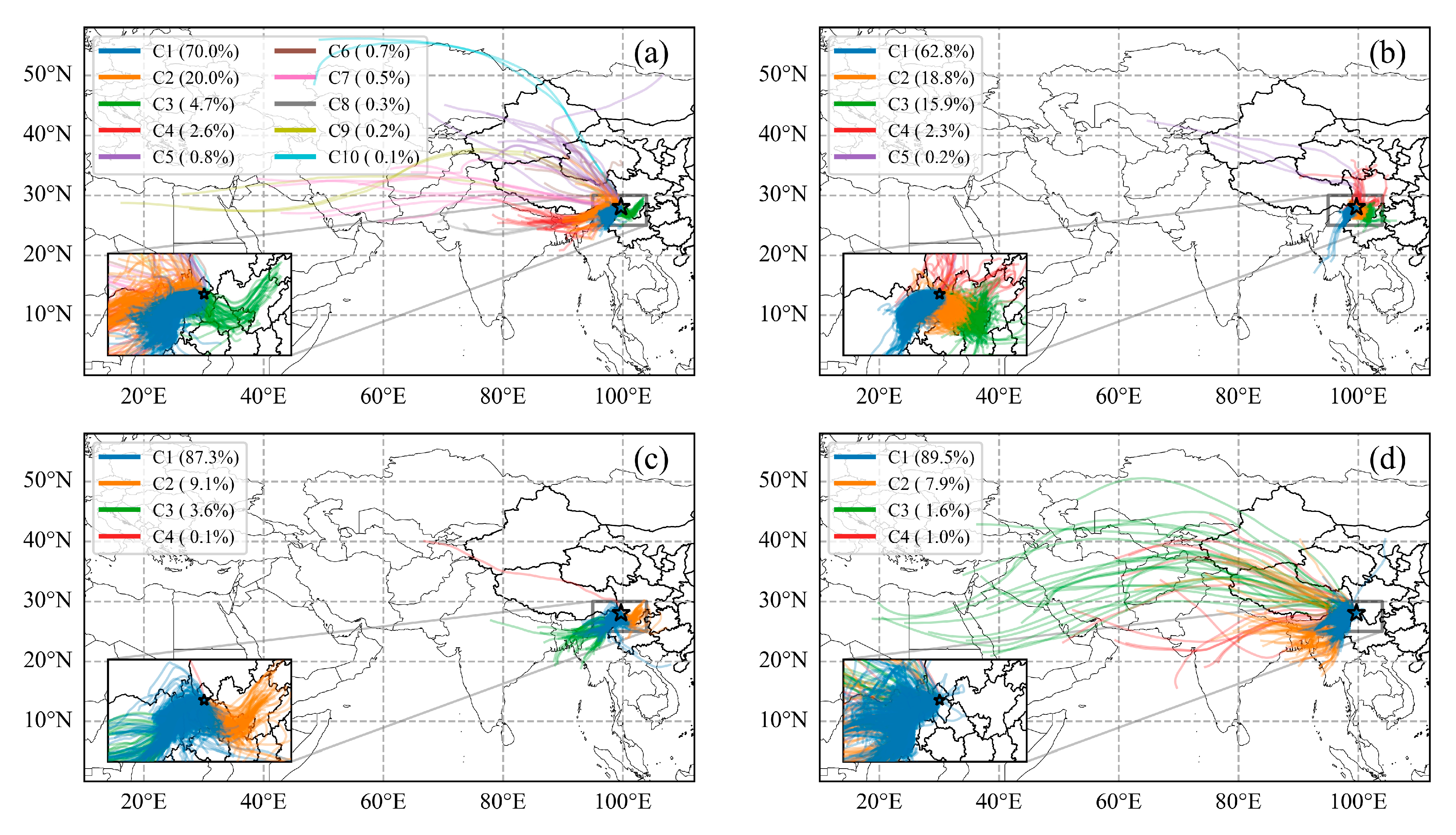
Backward 72 h trajectory analyses using the HYSPLIT model (Figure 5) delineate the seasonal origins of air masses arriving at Shangri-La, with trajectories clustered by transport path similarity. In spring, dominant clusters originate from the south, notably C1 (70.0%) and C2 (20.0%) from the Indo-Myanmar region, and C3 (4.7%) from southern Sichuan. A small number of trajectories also extended to remote sources such as North Africa and Central Asia. In summer, trajectories arrive predominantly from the east, including C1 (62.8%) from central and northern Myanmar, and C2 (18.8%) and C3 (15.9%) from the central Sichuan–Yunnan region. Autumn exhibits a pattern similar to spring, though with fewer long-range transports from the west: C1 (87.3%) and C3 (3.6%) originate from the Indo-Myanmar region, and C2 (9.1%) from southeastern Sichuan. In winter, influences are highly concentrated in the Indo-Myanmar region, represented by C1 (89.5%) and C2 (7.9%), with a limited number of air masses from North Africa and Central Asia. The clustering results confirm that air parcels arriving at the site originate mainly from westerly and southwestern directions, underscoring the strong influence of the westerlies and monsoon flows. Regional recirculation occurs in all seasons, supplemented by intermittent long-range transport in spring and winter.
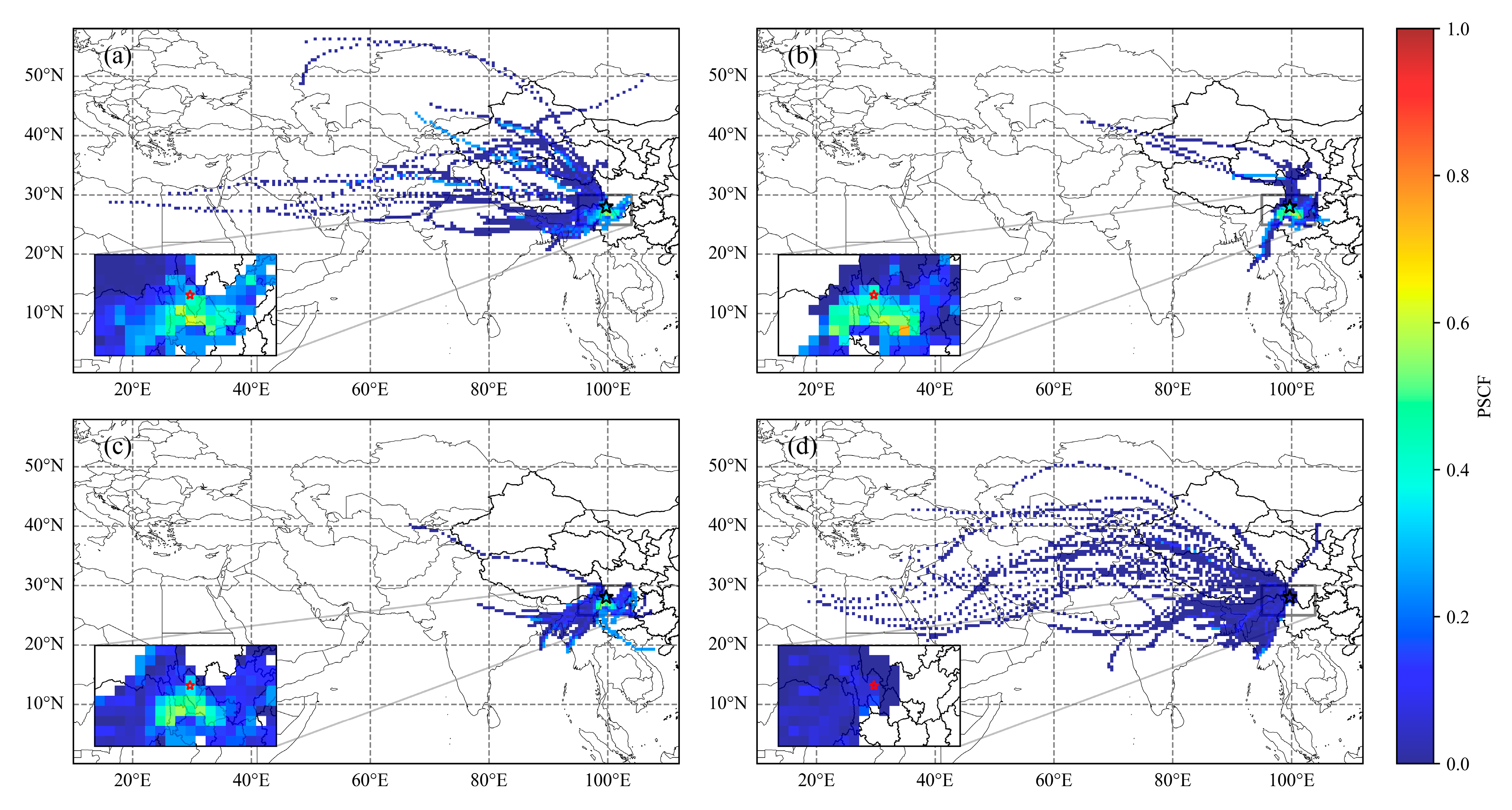
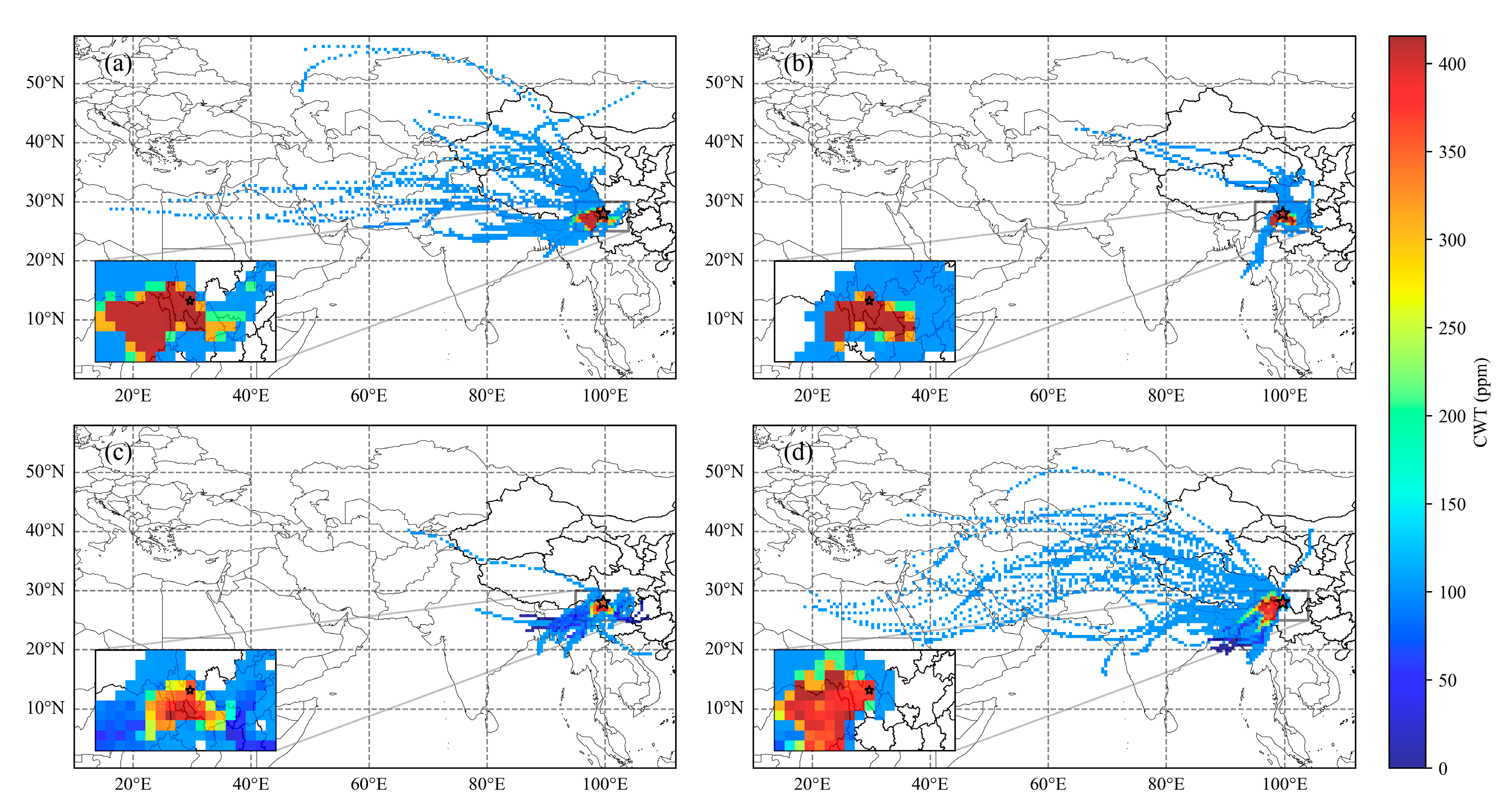
To further determine the potential emission sources for Shangri-La station, PSCF and CWT analyses for CO2 were jointly applied on 72 h backward trajectories, shown in Figure 6 and Figure 7, respectively. the PSCF results use data labeled as “pollution event” in the previous background extraction section. PSCF identifies areas with high probabilities of association with elevated CO2 events, while CWT quantifies their relative contributions by weighting each trajectory with the observed concentration. The PSCF and CWT results complement each other to distinguish where high-CO2 air masses originate and how strongly those regions contribute. The cells are colored according to the calculated PSCF probabilities and weighted concentrations, with the reddish parts illustrating a high probability of source locations and strong emission sources affecting the measurement site.
Based on the PSCF analysis, regions to the south (including southwest and southeast) of the monitoring site show a high probability of being potential CO2 sources in all seasons except winter, reflecting the persistent influence of nearby urban and agricultural activities. In spring, the highest probability of emission sources is found in the southern and southeastern sectors, which aligns with the transport pathways of clusters C1 and C3 in Figure 5. Air masses associated with these clusters are likely influenced by local emissions before reaching the sampling site. During summer and autumn, monsoon circulation transports residual anthropogenic emissions and biomass burning plumes, contributing to high PSCF values in southern regions [35,36]. In winter, however, the scarcity of pollution events leads to consistently low PSCF probabilities in all directions.
Based on the CWT analysis, elevated trajectory-weighted concentrations are predominantly observed in the vicinity of the measurement site, underscoring the dominance of regional emissions and transport in influencing CO2 levels at Shangri-La. The strong spatial agreement between PSCF and CWT results confirms the mutual consistency of the two methods and strengthens the credibility of the identified source regions. It is noteworthy that the CWT algorithm incorporates all observed concentrations, both high and low, and integrates contributions from all trajectories passing through a grid cell. Consequently, in directions with a high frequency of air mass arrivals (such as the southern pathways), the accumulated weighted concentration can be substantially elevated, even if individual trajectories do not always carry strongly polluted air masses.
Combining the trajectory clustering, PSCF and CWT methods, we observed that CO2 emission sources in Shangri-La mainly lie around it, especially in the south directions (e.g., Indo-Myanmar region, Lijiang City, and Panzhihua City). Compared to the PSCF results reported by Guo et al. (2020) [16], CO2 sources in the study period have shifted slightly toward the south and southeast of the station. The high degree of spatial overlap between PSCF and CWT patterns underscores their mutual consistency: PSCF pinpoints probable transport corridors, while CWT quantifies the relative intensity of those inflows. Their convergence validates the robustness of the source attribution and emphasizes that seasonal regional transport, rather than local emissions, governs most high-CO2 events at the station.

3.4. Wind Rose Analysis

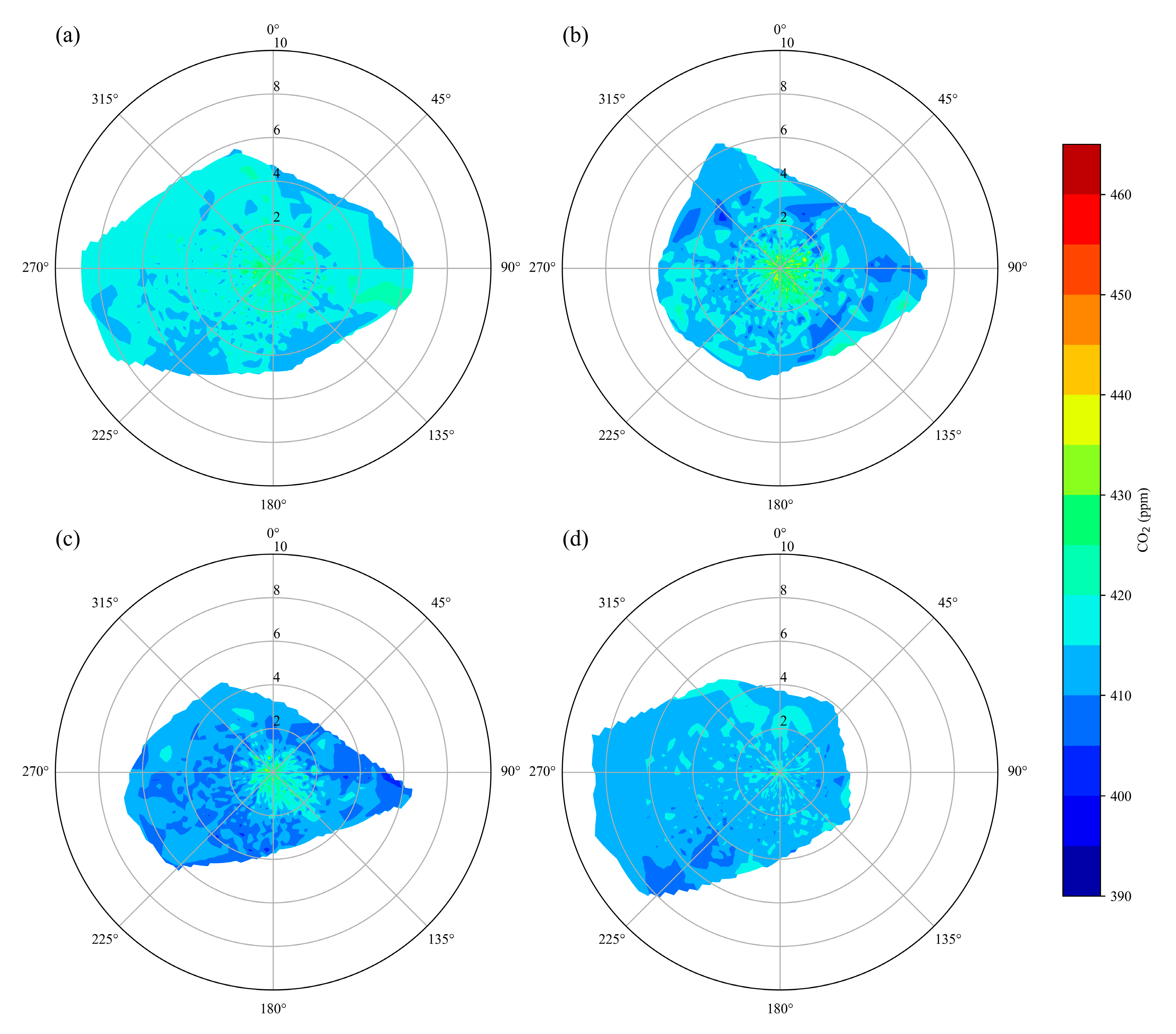
Wind rose distributions of CO2 concentration (Figure 8) provide additional insight into wind controls. Across all seasons, low wind speeds (<1.5 m s−1) correspond to elevated CO2 levels (>425 ppm), indicating accumulation under stagnant conditions. In spring, higher CO2 values are also associated with stronger winds from the west and southeast, suggesting that the elevated concentrations primarily arose from sources in the west and southeast regions, including northern Myanmar region and Sichuan Basin. During summer and autumn, higher CO2 occurs primarily under southeasterly winds, with additional summer peaks under southwesterly flow, consistent with monsoonal transport. In winter, no distinct wind direction preference is evident, though moderate enhancements (>410 ppm) appear under north-northwesterly flow, corresponding to the partial trajectories flowing in from the northwest in cluster C1 in Figure 5, while the highest wind speeds (~8 m s−1) are associated with southwesterly winds.

4. Conclusions

Continuous in situ measurements of CO2 at the Shangri-La background station from 2019 to 2022 provide updated assessment of CO2 variability over the southeastern Tibetan Plateau. The principal findings are summarized as follows:
(1)
The REBS-derived background CO2 increased from ~409 ppm in 2019 to ~417 ppm in 2022, corresponding to an annual growth rate of 1.9 ± 0.1 ppm yr−1. This is slightly lower than both the 2010–2014 rate at the same site and the global mean growth rate during the same period (~2.4 ppm yr−1 for 2019–2022 [1]), consistent with the recent ENSO-modulated slowdown in global CO2 accumulation.
(2)
A distinct seasonal cycle, with spring maxima and late-summer minima, reflects the joint influence of biospheric activity and monsoonal circulation. Pronounced diurnal amplitudes in summer (up to 25 ppm) indicate strong daytime photosynthetic drawdown and nighttime accumulation under stable stratification.
(3)
Integrated HYSPLIT–PSCF–CWT analyses reveal that regional transport dominates high-CO2 episodes. Air masses primarily originate from the southern Indo-Myanmar and Sichuan-Yunnan regions. Relative to 2010–2016, potential source influence has shifted slightly toward the south and southeast of the station.
It should be noted that the present dataset does not allow a strict quantitative attribution of the hourly or seasonal CO2 variability to individual processes such as terrain channeling, agricultural activities, biomass burning, traffic, or tourism emissions; such analyses would require numerical modeling and additional datasets. The physical interpretations provided here are therefore qualitative. Importantly, these uncertainties do not affect the robustness of the REBS-derived background time series and the dominant transport pathways identified in this study. Overall, these observations demonstrate that the Shangri-La station effectively captures both regional background CO2 and synoptic-scale transport signals, providing high-quality baseline data representative of the southeastern Tibetan Plateau. The integration of these in situ measurements with satellite observations and atmospheric inversion models will be vital for improving regional carbon fluxes estimates and understanding carbon–climate interactions in this complex terrain.

Author Contributions

Conceptualization, Y.Y. and R.Z.; methodology, R.Z.; software, R.Z.; validation, X.S., W.H., X.L. and C.Z.; formal analysis, Y.Y., X.S., W.H. and X.L.; investigation, Y.Y., X.D., X.P. and X.L.; resources, Y.Y.; data curation, X.S. and C.Z.; writing—original draft preparation, Y.Y., X.P. and X.D.; writing—review and editing, R.Z. and W.H.; visualization, Y.Y. and W.H.; supervision, Y.Y. and X.D.; project administration, Y.Y. and X.D.; funding acquisition, X.D. All authors have read and agreed to the published version of the manuscript.

Funding

This research was funded by the Yunnan Meteorological Bureau Research Project, grant number YZ202535 and the Post-acceptance Subsidy Funds for the Shangri-La Atmospheric Composition Yunnan Province Field Scientific Observation and Research Station in 2024 (2024–2025), grant number 202405AW340003.

Institutional Review Board Statement

Not applicable.

Informed Consent Statement

Not applicable.

Data Availability Statement

The data are available from the corresponding author on reasonable request.

Acknowledgments

The authors are grateful to the staff of the Shangri-La Atmospheric Background Station for their long-term maintenance of the monitoring instruments and data acquisition. We also acknowledge the NOAA Air Resources Laboratory (ARL) for providing the HYSPLIT model and GDAS meteorological data used in this study, and the World Data Centre for Greenhouse Gases (WDCGG) for providing Waliguan CO2 records and NOAA Global Monitoring Laboratory (GML) for providing greenhouse gas Marine Boundary Layer reference. Constructive comments from anonymous reviewers are greatly appreciated, which helped improve the clarity and quality of this manuscript.

Conflicts of Interest

The authors declare no conflicts of interest.

References

  1. WMO. WMO Greenhouse Gas Bulletin No. 21. Available online: https://wmo.int/publication-series/wmo-greenhouse-gas-bulletin-no-21 (accessed on 1 October 2025).
  2. Masson-Delmotte, V.; Zhai, P.; Pirani, A.; Connors, S.L.; Péan, C.; Berger, S.; Caud, N.; Chen, Y.; Goldfarb, L.; Gomis, M.I. Climate change 2021: The physical science basis. Contrib. Work. Group I Sixth Assess. Rep. Intergov. Panel Clim. Change 2021, 2, 2391. [Google Scholar]
  3. Friedlingstein, P.; O’Sullivan, M.; Jones, M.W.; Andrew, R.M.; Hauck, J.; Landschützer, P.; Le Quéré, C.; Li, H.; Luijkx, I.T.; Olsen, A.; et al. Global Carbon Budget 2024. Earth Syst. Sci. Data 2025, 17, 965–1039. [Google Scholar] [CrossRef]
  4. Houghton, R.A. Revised estimates of the annual net flux of carbon to the atmosphere from changes in land use and land management 1850–2000. Tellus B Chem. Phys. Meteorol. 2003, 55, 378–390. [Google Scholar]
  5. Conway, T.J.; Tans, P.P.; Waterman, L.S.; Thoning, K.W.; Kitzis, D.R.; Masarie, K.A.; Zhang, N. Evidence for interannual variability of the carbon cycle from the National Oceanic and Atmospheric Administration/Climate Monitoring and Diagnostics Laboratory Global Air Sampling Network. J. Geophys. Res. Atmos. 1994, 99, 22831–22855. [Google Scholar] [CrossRef]
  6. Keeling, R.F. Recording Earth’s Vital Signs. Science 2008, 319, 1771–1772. [Google Scholar] [CrossRef]
  7. Briber, B.M.; Hutyra, L.R.; Dunn, A.L.; Raciti, S.M.; Munger, J.W. Variations in atmospheric CO2 mixing ratios across a Boston, MA urban to rural gradient. Land 2013, 2, 304–327. [Google Scholar] [CrossRef]
  8. Conway, T.J.; Tans, P.P.; BBoden, T. Atmospheric Carbon Diooxide Mixing Ratios from the NOAA Climate Monitoring and Diagnostics Laboratory Cooperative Flask Sampling Network, 1967–1993; Oak Ridge National Lab. (ORNL): Oak Ridge, TN, USA, 1996.
  9. Keeling, C.D.; Bacastow, R.B.; Bainbridge, A.E.; Ekdahl, C.A., Jr.; Guenther, P.R.; Waterman, L.S.; Chin, J.F. Atmospheric carbon dioxide variations at Mauna Loa observatory, Hawaii. Tellus 1976, 28, 538–551. [Google Scholar] [CrossRef]
  10. Zhou, L.; Conway, T.J.; White, J.W.; Mukai, H.; Zhang, X.; Wen, Y.; Li, J.; MacClune, K. Long-term record of atmospheric CO2 and stable isotopic ratios at Waliguan Observatory: Background features and possible drivers, 1991–2002. Glob. Biogeochem. Cycles 2005, 19, GB3021. [Google Scholar] [CrossRef]
  11. Ballantyne, A.á.; Alden, C.á.; Miller, J.á.; Tans, P.á.; White, J. Increase in observed net carbon dioxide uptake by land and oceans during the past 50 years. Nature 2012, 488, 70–72. [Google Scholar] [CrossRef] [PubMed]
  12. Graven, H.; Keeling, R.; Piper, S.; Patra, P.; Stephens, B.; Wofsy, S.; Welp, L.; Sweeney, C.; Tans, P.; Kelley, J. Enhanced seasonal exchange of CO2 by northern ecosystems since 1960. Science 2013, 341, 1085–1089. [Google Scholar] [CrossRef]
  13. Mai, B.; Deng, X.; Zhang, F.; He, H.; Luan, T.; Li, F.; Liu, X. Background Characteristics of Atmospheric CO2 and the Potential Source Regions in the Pearl River Delta Region of China. Adv. Atmos. Sci. 2020, 37, 557–568. [Google Scholar] [CrossRef]
  14. Liu, L.; Zhou, L.; Zhang, X.; Wen, M.; Zhang, F.; Yao, B.; Fang, S. The characteristics of atmospheric CO2 concentration variation of four national background stations in China. Sci. China Ser. D Earth Sci. 2009, 52, 1857–1863. [Google Scholar] [CrossRef]
  15. Fang, S.; Tans, P.P.; Steinbacher, M.; Zhou, L.; Luan, T.; Li, Z. Observation of atmospheric CO2 and CO at Shangri-La station: Results from the only regional station located at southwestern China. Tellus B Chem. Phys. Meteorol. 2016, 68, 28506. [Google Scholar] [CrossRef]
  16. Guo, M.; Fang, S.; Liu, S.; Liang, M.; Wu, H.; Yang, L.; Li, Z.; Liu, P.; Zhang, F. Comparison of atmospheric CO2, CH4, and CO at two stations in the Tibetan Plateau of China. Earth Space Sci. 2020, 7, e2019EA001051. [Google Scholar] [CrossRef]
  17. Liu, J.; Bowman, K.W.; Schimel, D.S.; Parazoo, N.C.; Jiang, Z.; Lee, M.; Bloom, A.A.; Wunch, D.; Frankenberg, C.; Sun, Y.; et al. Contrasting carbon cycle responses of the tropical continents to the 2015–2016 El Niño. Science 2017, 358, eaam5690. [Google Scholar] [CrossRef] [PubMed]
  18. Chen, B.; Chao, W.C.; Liu, X. Enhanced climatic warming in the Tibetan Plateau due to doubling CO2: A model study. Clim. Dyn. 2003, 20, 401–413. [Google Scholar] [CrossRef]
  19. Li, T.; Wang, Y.; Wang, B.; Ting, M.; Ding, Y.; Sun, Y.; He, C.; Yang, G. Distinctive South and East Asian monsoon circulation responses to global warming. Sci. Bull. 2022, 67, 762–770. [Google Scholar] [CrossRef]
  20. Tiwari, Y.K.; Vellore, R.K.; Ravi Kumar, K.; van der Schoot, M.; Cho, C.-H. Influence of monsoons on atmospheric CO2 spatial variability and ground-based monitoring over India. Sci. Total Environ. 2014, 490, 570–578. [Google Scholar] [CrossRef]
  21. Ruckstuhl, A.F.; Henne, S.; Reimann, S.; Steinbacher, M.; Vollmer, M.K.; O’Doherty, S.; Buchmann, B.; Hueglin, C. Robust extraction of baseline signal of atmospheric trace species using local regression. Atmos. Meas. Technol. 2012, 5, 2613–2624. [Google Scholar] [CrossRef]
  22. Cheng, X.L.; Liu, X.M.; Liu, Y.J.; Hu, F. Characteristics of CO2 Concentration and Flux in the Beijing Urban Area. J. Geophys. Res. Atmos. 2018, 123, 1785–1801. [Google Scholar] [CrossRef]
  23. Wang, S.; Zhu, L.; Yan, S.; Li, Y.; Wang, W.; Gao, X.a.; Ma, Z.; Liu, P.; Liang, M. Atmospheric CO2 Data Filtering Method and Characteristics of the Mole Fractions at Wutaishan Station in Shanxi of China. Aerosol Air Qual. Res. 2020, 20, 2953–2962. [Google Scholar] [CrossRef]
  24. Wu, D.; Yue, Y.; Jing, J.; Liang, M.; Sun, W.; Han, G.; Lou, M. Background Characteristics and Influence Analysis of Greenhouse Gases at Jinsha Atmospheric Background Station in China. Atmosphere 2023, 14, 1541. [Google Scholar] [CrossRef]
  25. Stein, A.F.; Draxler, R.R.; Rolph, G.D.; Stunder, B.J.B.; Cohen, M.D.; Ngan, F. NOAA’s HYSPLIT Atmospheric Transport and Dispersion Modeling System. Bull. Am. Meteorol. Soc. 2015, 96, 2059–2077. [Google Scholar] [CrossRef]
  26. Kabashnikov, V.P.; Chaikovsky, A.P.; Kucsera, T.L.; Metelskaya, N.S. Estimated accuracy of three common trajectory statistical methods. Atmos. Environ. 2011, 45, 5425–5430. [Google Scholar] [CrossRef]
  27. Lan, L.; Ghasemifard, H.; Yuan, Y.; Hachinger, S.; Zhao, X.; Bhattacharjee, S.; Bi, X.; Bai, Y.; Menzel, A.; Chen, J. Assessment of Urban CO2 Measurement and Source Attribution in Munich Based on TDLAS-WMS and Trajectory Analysis. Atmosphere 2020, 11, 58. [Google Scholar] [CrossRef]
  28. Mai, B.; Deng, X.; Liu, X.; Li, T.; Guo, J.; Ma, Q. The climatology of ambient CO2 concentrations from long-term observation in the Pearl River Delta region of China: Roles of anthropogenic and biogenic processes. Atmos. Environ. 2021, 251, 118266. [Google Scholar] [CrossRef]
  29. Pathakoti, M.; Kanchana, A.L.; Mahalakshmi, D.V.; Guha, T.; Raja, P.; Nalini, K.; Rajan, K.S.; Sesha Sai, M.V.R.; Dadhwal, V.K. Implications of Emission Sources and Biosphere Exchange on Temporal Variations of CO2 and δ13C Using Continuous Atmospheric Measurements at Shadnagar (India). J. Geophys. Res. Atmos. 2023, 128, e2022JD036472. [Google Scholar] [CrossRef]
  30. Metya, A.; Datye, A.; Chakraborty, S.; Tiwari, Y.K.; Sarma, D.; Bora, A.; Gogoi, N. Diurnal and seasonal variability of CO2 and CH4 concentration in a semi-urban environment of western India. Sci. Rep. 2021, 11, 2931. [Google Scholar] [CrossRef]
  31. Betts, R.A.; Jones, C.D.; Knight, J.R.; Keeling, R.F.; Kennedy, J.J. El Niño and a record CO2 rise. Nat. Clim. Change 2016, 6, 806–810. [Google Scholar] [CrossRef]
  32. WMO. WMO Greenhouse Gas Bulletin No. 20. Available online: https://wmo.int/publication-series/wmo-greenhouse-gas-bulletin-no-20 (accessed on 1 October 2025).
  33. Shen, M.; Piao, S.; Chen, X.; An, S.; Fu, Y.H.; Wang, S.; Cong, N.; Janssens, I.A. Strong impacts of daily minimum temperature on the green-up date and summer greenness of the Tibetan Plateau. Glob. Change Biol. 2016, 22, 3057–3066. [Google Scholar] [CrossRef]
  34. Zhang, G.; Zhang, Y.; Dong, J.; Xiao, X. Green-up dates in the Tibetan Plateau have continuously advanced from 1982 to 2011. Proc. Natl. Acad. Sci. USA 2013, 110, 4309–4314. [Google Scholar] [CrossRef] [PubMed]
  35. Liang, Y.; Gui, K.; Zheng, Y.; Yang, X.; Li, X.; Liu, C.; Sheng, Z.; Sun, T.; Zhang, X.; Che, H. Impact of Biomass Burning in South and Southeast Asia on Background Aerosol in Southwest China. Aerosol Air Qual. Res. 2019, 19, 1188–1204. [Google Scholar] [CrossRef]
  36. Zheng, J.; Hu, M.; Du, Z.; Shang, D.; Gong, Z.; Qin, Y.; Fang, J.; Gu, F.; Li, M.; Peng, J.; et al. Influence of biomass burning from South Asia at a high-altitude mountain receptor site in China. Atmos. Chem. Phys. 2017, 17, 6853–6864. [Google Scholar] [CrossRef]
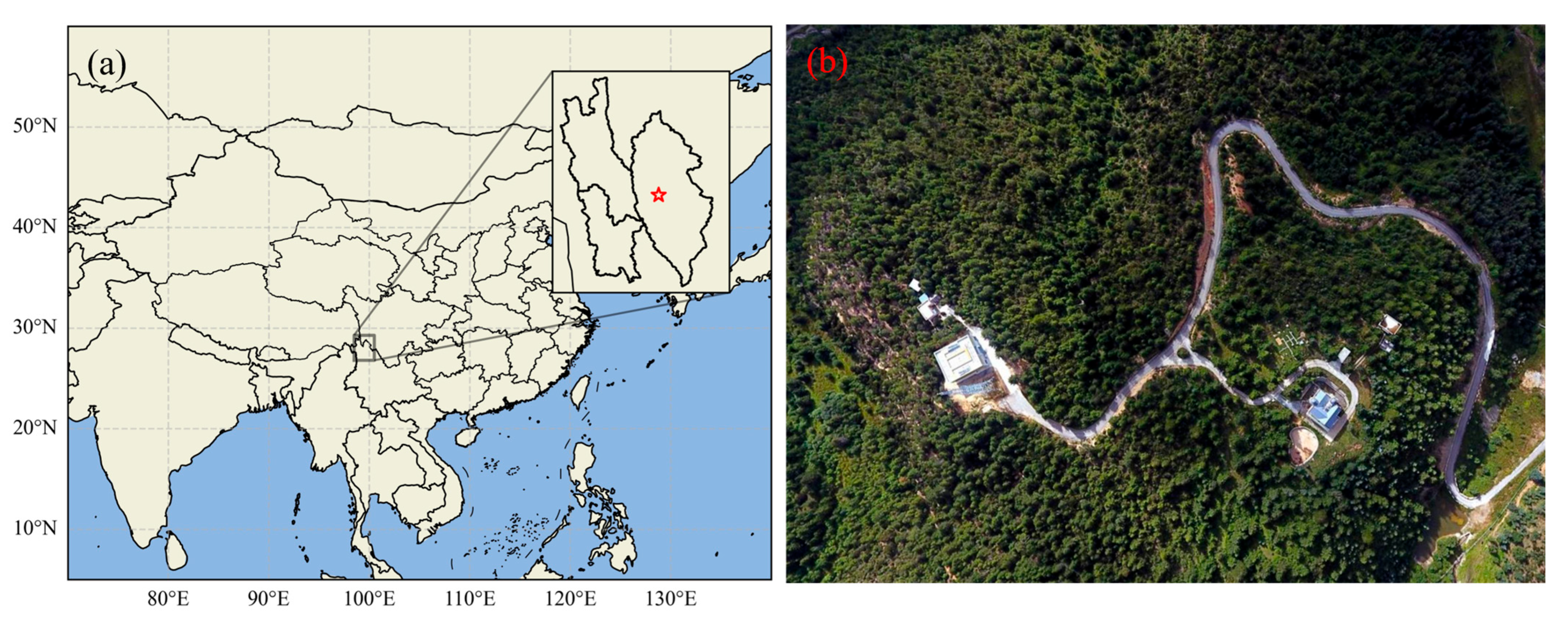
Figure 1. (a) The geographical location of the Shangri-La station. (b) A bird’s-eye view of the station and its immediate surroundings.
Atmosphere 17 00003 g001
Figure 2. Monthly diurnal cycle of atmospheric CO2 measured at the Shangri-La station, presented in Coordinated Universal Time (UTC). Subplots (al) correspond to the months from January to December, respectively. The red line traces the modal value for each hour. The boxes depict the data distribution from the first quartile (Q1) to the third quartile (Q3), with the median marked internally. The whiskers show the data range within 1.5 times the interquartile range (IQR). Outliers (gray dots) are defined as values: >Q3 + 1.5 × IQR or <Q1 − 1.5 × IQR. The gray shaded areas correspond to the local nighttime at the station, calculated by longitude, latitude, and altitude of the station.
Atmosphere 17 00003 g002
Figure 3. Time series of atmospheric CO2 at the Shangri-La station (2019–2022) The gray line represents the observed concentrations. The solid green line denotes the REBS (Robust Extraction of Baseline Signal) baseline. The shaded area between the orange dash-dotted lines defines the background variability (baseline ± 2σ). Notable pollution events and depletion events are highlighted as blue and red dots, respectively. Short-term signals exceeding this range are identified as pollution (blue dots) or depletion (red dots) events. The long-term trend is indicated by the sky-blue dashed line.
Atmosphere 17 00003 g003
Figure 4. Monthly background CO2 of global (blue line) and at Mt. Waliguan (orange line, WLG) and Shangri-La (green line, XGLL) station.
Atmosphere 17 00003 g004
Figure 5. Seasonal clusters of 72 h backward trajectories arriving at the Shangri-La station (black star) from 2019 to 2022 at 00, 06, 12, 18 UTC: (a) spring, (b) summer, (c) autumn, and (d) winter. Number of trajectories in each season is approximately 1440. The trajectories were calculated using the HYSPLIT model. Each line represents an individual trajectory, colored according to its assigned cluster where trajectories are with similar transport pathways, and the percentage value indicates the relative frequency of each cluster. The inset focuses on the regional context of the station (95° E–104° E, 25° N–30° N).
Atmosphere 17 00003 g005
Figure 6. Potential source contribution function (PSCF) results for CO2 in the region, based on 72-h backward trajectories, showing the likely emission source regions by season: (a) spring, (b) summer, (c) autumn, and (d) winter. Red areas indicate grid cells with a high probability of being CO2 sources, while blue areas denote grid cells with a low probability. The receptor site is marked by a red star. The inset focuses on the regional context of the station (95° E–104° E, 25° N–30° N).
Atmosphere 17 00003 g006
Figure 7. Concentration Weighted Trajectory (CWT) results for CO2 in the region, based on 72-h backward trajectories, showing the estimated contribution of potential source areas by season: (a) spring, (b) summer, (c) autumn, and (d) winter. Red areas indicate grid cells with high-weighted concentrations, signifying strong potential source contributions, while blue areas denote grid cells with low-weighted concentrations, indicating weak source contributions. The receptor site is marked by a black star. The inset focuses on the regional context of the station (95° E–104° E, 25° N–30° N).
Atmosphere 17 00003 g007
Figure 8. Seasonal wind roses of raw CO2 concentration at the Shangri-La station: (a) spring, (b) summer, (c) autumn, and (d) winter. The concentric circles represent wind speed ranges (units: m s−1), the azimuth indicates the wind direction, and the color shaded areas show the grid interpolated CO2 concentration.
Atmosphere 17 00003 g008
Disclaimer/Publisher’s Note: The statements, opinions and data contained in all publications are solely those of the individual author(s) and contributor(s) and not of MDPI and/or the editor(s). MDPI and/or the editor(s) disclaim responsibility for any injury to people or property resulting from any ideas, methods, instructions or products referred to in the content.