Forecasting ⁷Be Concentrations Using Time Series Analysis: A Case Study of Panama City

Abstract

Beryllium-7 (⁷Be) is widely used as an atmospheric radiotracer due to its short half-life and ease of detection. Its evaluation and forecasting provide valuable insights into atmospheric behavior and environmental processes. This study aimed to develop a robust explanatory and predictive model for ⁷Be concentrations in Panama using monthly data from 2006 to 2019 provided by the RN50 Station at the University of Panama. This study employed ARIMA models for time series analysis and forecasting, complemented by error metrics such as Root Mean Squared Error (RMSE), Mean Squared Error (MSE), Mean Absolute Error (MAE), and Mean Absolute Percentage Error (MAPE) to assess the accuracy of the results. After verifying data suitability, analyzing series components, and testing stationarity using the Dickey–Fuller test, the SARIMA (2,0,1) (2,1,0) model was identified as optimal. This model successfully forecasted ⁷Be concentrations for the final five months of 2019, offering a useful tool for understanding airborne particle dynamics in Panama and supporting future applications of ⁷Be in the study and estimation of soil erosion.

1. Introduction

Beryllium-7 (⁷Be) is a naturally occurring cosmogenic radionuclide formed mainly in the stratosphere (~70%) and, to a lesser extent, in the troposphere [1,2], through interactions between cosmic rays or energetic solar particles and nuclei of atmospheric nitrogen, oxygen, and carbon [3,4,5,6]. Its production depends on the flux of cosmic rays, which varies according to latitude, altitude, and solar activity, increasing from the equator toward the poles and reaching maximum values at altitudes between 12 and 20 km before decreasing exponentially toward the Earth’s surface [7,8].

During periods of maximum solar activity, the amount of cosmic rays reaching Earth decreases as a result of the solar wind reinforcing the heliosphere, generating a shield that scatters and deflects cosmic rays, hindering their entry and reducing the amount that reaches the Earth’s atmosphere [9,10,11,12], which reduces the production of ⁷Be. After its formation, ⁷Be rapidly attaches to submicrometer-sized atmospheric aerosols (0.4–2 μm) [6,13,14,15] and is subsequently removed from the atmosphere through wet deposition (rain, snow) or dry deposition driven by gravity [4]. Wet deposition is the dominant pathway for its transfer to the Earth’s surface, where it binds strongly to soil and vegetation particles [14,16,17]. ⁷Be in the atmosphere is transported to the earth’s surface by precipitation events, and its concentrations are used to study the erosive processes that soil undergoes as a result of specific and extreme rainfall events. In tropical urban environments such as Panama City, atmospheric aerosols (PM₁₀) originate from both natural and anthropogenic sources. Natural aerosols include marine spray and mineral dust transported from distant deserts such as the Sahara, while anthropogenic contributions primarily stem from industrial activity, construction, and vehicular emissions [18]. In northern Morocco, the seasonal dynamics of aerosols show the interaction between local emissions, meteorological conditions, and continental atmospheric transport of air masses laden with pollutants [19]. These suspended particles influence solar irradiance at the surface; similarly, factors such as insolation, precipitation, and temperature affect local climate and weather conditions [20,21], which could modulate the deposition dynamics of ⁷Be.

The mean residence time of ⁷Be in the lower atmosphere is about 8 days, and precipitation frequency plays a key role in its removal [22]. ⁷Be has a half-life of 53.3 days and decays primarily by electron capture to lithium, either directly to the ground state (89.56%) or to an excited state that emits gamma radiation at 477.6 keV [23]. Its atmospheric concentration is not homogeneous and is influenced by factors such as geographical location, solar activity, atmospheric circulation, vertical mixing, and removal efficiency [24]. Seasonal and geographical patterns have been observed: in tropical and equatorial regions, high precipitation rates produce strong correlations between ⁷Be activity and rainfall, whereas in mid-latitudes both solar activity and meteorological phenomena play important roles; in polar regions, correlations with precipitation are absent [25], indicating that dry deposition, turbulent mixing, and solar activity are dominant.

Due to its continuous replenishment from the atmosphere, restriction to the surface soil layer, and straightforward detection by gamma-ray spectrometry, ⁷Be has become a widely used environmental tracer. Applications include studies of atmospheric transport, air mass origins, vertical tropospheric exchange, particle removal, coastal sediment recovery, and, more recently, quantification of soil erosion and sediment redistribution [26,27,28,29,30,31]. Short-term soil erosion studies are of growing interest given the increased frequency of extreme rainfall events associated with global climate change [32,33]

In this study, atmospheric ⁷Be concentration data collected by the RN50 Station, located at the University of Panama in Panama City, are analyzed. The station is geographically positioned at latitude 8°59′00.9″ N (8.984° N) and longitude 79°31′59.1″ W (79.533° W), at an elevation of 90 m above sea level, within a tropical urban environment influenced by both maritime and continental air masses. Daily ⁷Be activity concentrations recorded during the study period (2006–2019) exhibited marked interannual and intra-annual variability, reflecting the combined effects of seasonal precipitation patterns, aerosol dynamics, and regional meteorological conditions.

This study aims to apply time series models to forecast atmospheric ⁷Be concentrations in Panama City. The scope of the research focuses on characterizing temporal patterns and their applicability to environmental monitoring, considering that accurate forecasts allow anticipation of seasonal variations and extreme events, optimization of atmospheric dispersion models, and support for studies on air quality and climate change. To achieve this objective, we evaluate and compare the predictive performance of various Seasonal Autoregressive Integrated Moving Average (SARIMA) models to identify the most suitable approach for medium-term forecasting. The optimal model was selected based on error metric analysis, which allowed us to compare the accuracy of the estimates.

The paper is organized into four sections: Section 1 provides an introduction to the topic; Section 2 describes the methodology used; Section 3 presents the results; and Section 4 discusses the findings and conclusions of the research.

2. Materials and Methods

2.1. Data Description

⁷Be concentration data were provided by the RN50 Station is a member of the International Monitoring System (IMS) of the Comprehensive Nuclear-Test-Ban Treaty Organization, located at the University of Panama (8°59′00.9′′ N; 79°31′59.1′′ W) at an altitude of 90 m asl [34]. The station consists of an air particle sampler (Senya JL900; SENYA Ltd., Järvenpää, Finland) with the following characteristics:

• A 570 mm × 460 mm polypropylene filter (3M, Saint Paul, MN, USA).
• Collection efficiency of 99.99% for particles with a diameter equal to or greater than 0.4 μm and 85% for particles with a diameter between 0.15 and 0.4 μm, at a flow rate of 980 m³ h⁻¹ [35].

The filter is replaced at 6:00 AM daily after a 24 h monitoring period. To ensure the geometry of the sample to be analyzed, the filter is compressed in a mold that produces tablets with a diameter of 50.0 mm and a thickness of 5.0 mm. Finally, a Canberra GC5020 gamma spectrometer (Canberra Industries, Meriden, CT, USA) with a resolution of 1.93 keV and a relative efficiency of 56.1% at a gamma peak of 1.33 MeV from 60Co is used to determine the activity of ⁷Be. The total counting time interval ranged from 86,000 to 180,000 s. The minimum detectable concentration (MDC) was approximately 18 μBq m^–3. This dataset has a monthly frequency and spans 14 years, from January 2006 to July 2019, as shown in

Table 1. Variables of study.

Variable	Definition
Beryllium-7	Airborne particulate matter (PM10) samples were collected, and particulate analysis provided monthly measurements of Beryllium-7.
Year	Study period in years for Beryllium-7 concentrations: from 2006 to 2019.
Month	Study period (months) of Beryllium-7 concentrations: January 2006–July 2019.

. It is important to note that the reported daily data are the result of radiometric measurements taken on each collected filter [34].

2.2. Methodology

For the data analysis, statistical methods aligned with the study’s objectives and hypotheses were employed, following the Box and Jenkins methodology (Figure 1) [35].

This methodology enables the identification, estimation, validation, and generation of forecasts from SARIMA models. The main idea of the SARIMA model is to transform a time series into a stationary one, thereby turning it into a purely random process, in order to properly fit a forecasting model [36,37,38]. The modeling of the SARIMA process combines non-seasonal and seasonal components through four techniques: Autoregression (AR), Differencing (I), Moving Average (MA), and their seasonal counterparts. Autoregression explores the relationship between the variable and its lagged values; differencing seeks to stabilize the series by removing trends or seasonal patterns through differences between successive observations; and the moving average uses past forecast errors to estimate future values. The seasonal component captures periodic patterns in the series by adjusting lags and errors within defined cycles.

The general form of the ARIMA model is described in terms of the parameters p, d, q, which define the order of the autoregressive component, the degree of differencing, and the order of the moving average component, respectively. Hence, the notation ARIMA (p,d,q). The mathematical formulation of the ARIMA model is as follows:

$$y_t-y_{t-1}={\varphi }_1{y}_{t-1}+{\varphi }_2{y}_{t-2}+\cdots + {\varphi }_p{y}_{t-p}+ a_{t }-{\theta }_1{a}_{t-1}- {\theta }_2{a}_{t-2}-\cdots -{\theta }_q{a}_{t-q}$$

where

$p$ represents the autoregressive order;

$d$ is the degree of differencing;

$q$ is the moving average order;

$y_t$ is the value of the time series at time;

$t$ is an error term;

${\varphi }_1\dots {\varphi }_p$ are the autoregressive coefficients;

${\theta }_1\dots {\theta }_q$ are the moving average coefficients.

The analysis began with a review of the data to confirm its suitability for time series modeling by examining its components. Subsequently, the stationarity of the series was assessed using the Dickey–Fuller unit root test. Since the test indicated that the series was stationary, no differencing was required in the regular part; it was applied only to the seasonal component. This allowed for the formulation of an Autoregressive Integrated Moving Average SARIMA (p, d, q) (P, D, Q) model. Several predictive models were evaluated to estimate Beryllium-7 concentrations, and the selected SARIMA model was validated to generate forecasts for the last six months of 2019.

The modeling process followed a structured sequence, outlined in the following nine steps:

Step 1:

The modeling begins with an exploratory analysis of the beryllium concentration time series, in order to identify patterns such as trends, seasonality, and irregularities. Visualization tools, statistical tests, and correlograms were employed.

Step 2:

The Dickey–Fuller test was applied to assess mean stationarity, and it was necessary to apply differencing to stabilize the seasonal component of the series.

Step 3:

At this stage, the Levene test was applied as a reference to explore the homogeneity of variance in the series. Since no significant differences were detected between temporal segments, the variance was considered stable, suggesting variance stationarity. Therefore, no additional transformations were necessary to stabilize it.

Step 4:

To identify the SARIMA model parameters, the simple (ACF) and partial (PACF) correlograms were analyzed, which allowed establishing the initial values of the non-seasonal components (p, d, q) and seasonal components (P, D, Q).

Step 5:

Based on the structure observed in the correlograms and the results of the stationarity tests, different SARIMA model configurations were proposed, adjusting the parameters (p, d, q) (P, D, Q) to adequately capture the temporal dynamics of the beryllium series.

Step 6:

The performance of the models was evaluated using error metrics such as ME, RMSE, MAE, MAPE, and MASE, as detailed in

Table 2. Definition of the error metrics.

Metric	Formula	Description
ME (Mean Error)	$ME={\displaystyle \frac{1}{n}}{\displaystyle \sum _{t=1}^n}\left(y_t-{\widehat{y}}_t\right)$	Measures the average deviation between predicted and observed values.
RMSE (Root Mean Squared Error)	$RMSE=\sqrt{{\displaystyle \frac{1}{n}}{\displaystyle \sum _{t=1}^n}{{(y}_t-{\widehat{y}}_t)}^2}$	Provides information about the overall prediction accuracy.
MAE (Mean Absolute Error)	$MAE={\displaystyle \frac{1}{n}}{\displaystyle \sum _{t=1}^n}\left|y_t-{\widehat{y}}_t\right|$	Captures the average magnitude of errors, regardless of direction.
MPE (Mean Percentage Error)	$MPE={\displaystyle \frac{1}{n}}{\displaystyle \sum _{t=1}^n}{\displaystyle \frac{{(y}_t-{\widehat{y}}_t)}{y_t}}$	Indicates the average percentage deviation, useful for scale-independent comparisons
MAPE (Mean Absolute Percentage Error)	$MAPE={\displaystyle \frac{1}{n}}{\displaystyle \sum _{t=1}^n}\left|{\displaystyle \frac{{(y}_t-{\widehat{y}}_t)}{y_t}}\right|$	Expresses the error in percentage terms, facilitating comparison across different dataset.
MASE (Mean Absolute Scaled Error)	$MASE={\displaystyle \frac{\frac{1}{n}{\sum }_{t=1}^n\left|y_t-{\widehat{y}}_t\right|}{\frac{1}{n-1}\sum _{t=2}^n\left|y_t-{\widehat{y}}_{t-1}\right|}}$	An error metric that allows comparison across models by benchmarking against a naïve forecast. A naïve forecast assumes that the future value will be equal to the last observed value.

.

Step 7:

The selected models were validated by verifying that their estimated parameters were statistically significant.

Step 8:

The model’s performance was validated by checking that the residuals exhibited a white noise structure. Visualization tools and the Ljung–Box test were used.

Step 9:

Once the optimal model was selected, it was used to generate forecasts for the ⁷Be.

Data processing and analysis were conducted using the R programming language with the RStudio graphical interface, version 4.2.1 [39].

2.3. Error Metrics

Error measures in time series forecasting are used to compare the effectiveness of the applied models [40,41]. In general, the preferred model is the one with the lowest values in these metrics, as this indicates a better fit [42,43,44]. In this study, six error metrics were employed to evaluate the performance of the forecasting models, as defined in Table 2.

3. Results

This section presents the statistical results obtained from the time series analysis. The analysis of the historical data begins with the decomposition of the original time series to identify its underlying behavior, including trend and seasonal patterns (Figure 2).

Figure 2 reveals pronounced cyclical fluctuations with recurring peaks and troughs, indicating a strong seasonal component. Although the variability is considerable, no sustained upward or downward trend is observed, which may suggest mean stationarity. These characteristics highlight the importance of selecting a modeling approach capable of capturing both the seasonal dynamics and the stochastic nature of the data.

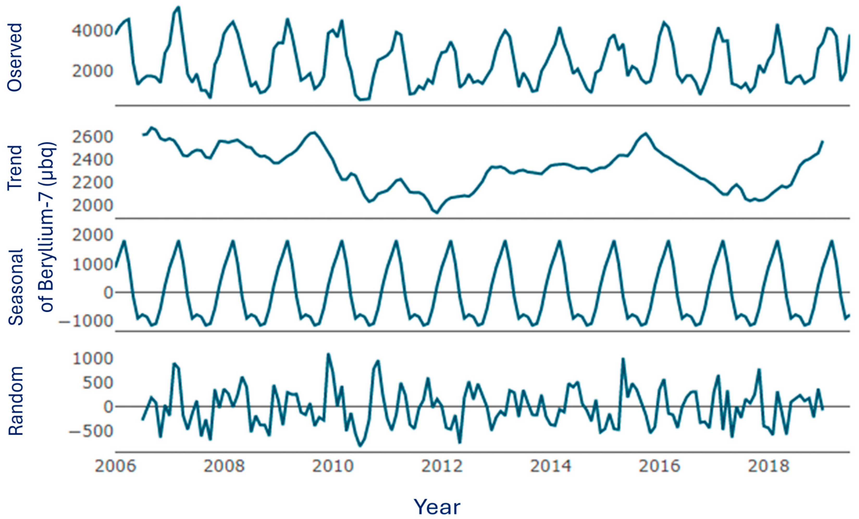
Figure 3 shows the decomposition of the series using the additive model, reinforcing the previous assumptions. The advantage of this decomposition is that it separates the seasonal component from the trend, allowing the behavior of the series to be observed more clearly.

Figure 3 displays, in the usual order, the observed values of the series, the trend, the seasonal variations, and the random fluctuations. Fluctuations in ⁷Be concentrations are evident; however, there is no linear trend throughout the study period, suggesting that the series is mean-stationary. On the other hand, the seasonal component is strong and pronounced. It is worth noting that the random part represents the configuration of the residuals left by the model, reflecting periods of decrease and increase.

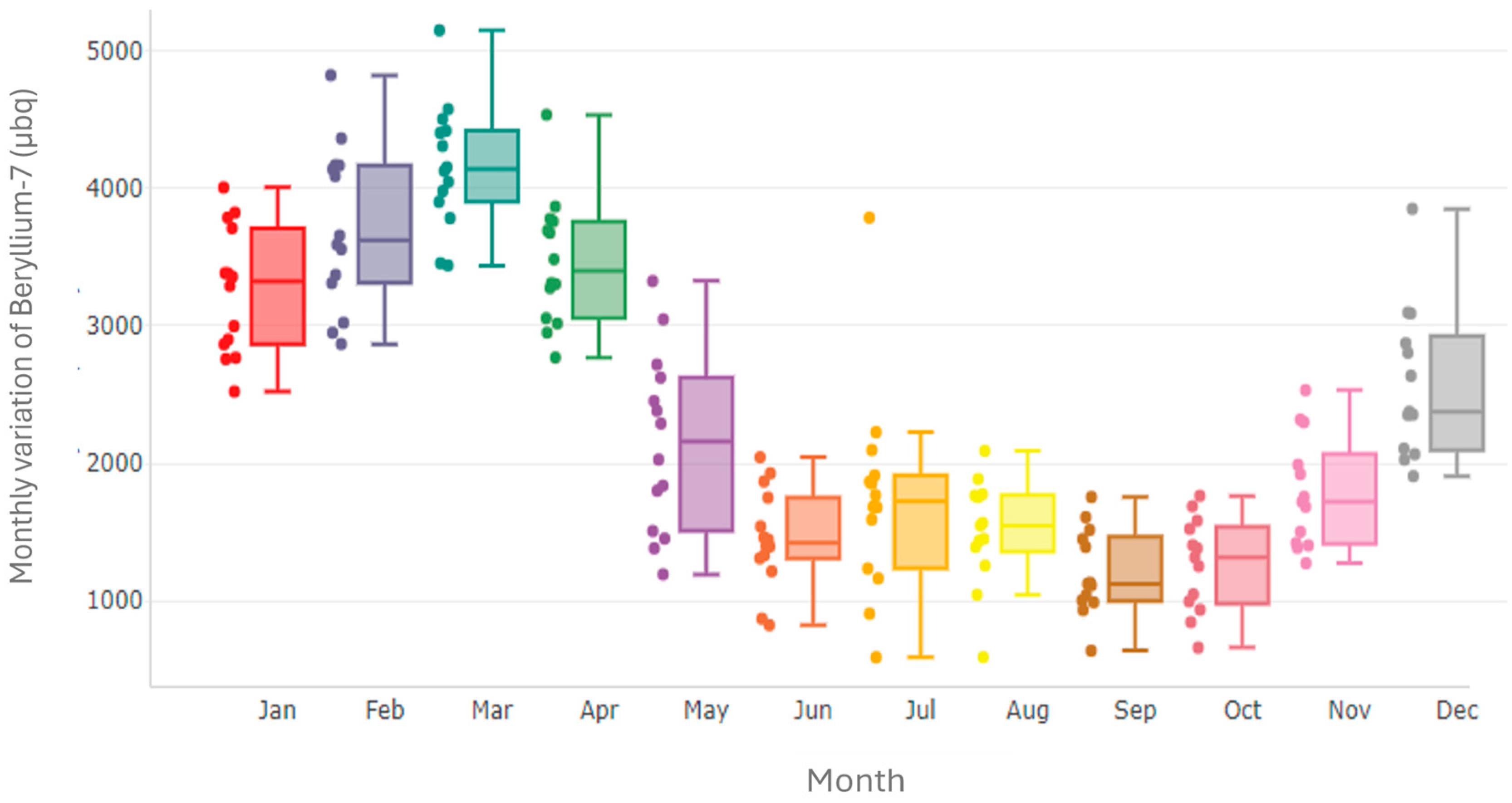
Figure 4 presents the seasonality plot of the Beryllium-7 time series, showing the monthly distribution of values using box plots.

As shown in Figure 4, the data exhibit a clear seasonal trend. Concentrations peak early in the year, especially during February and March, then gradually decline through December. Interestingly, there is a slight rebound at the end of the year, suggesting a recurring annual cycle.

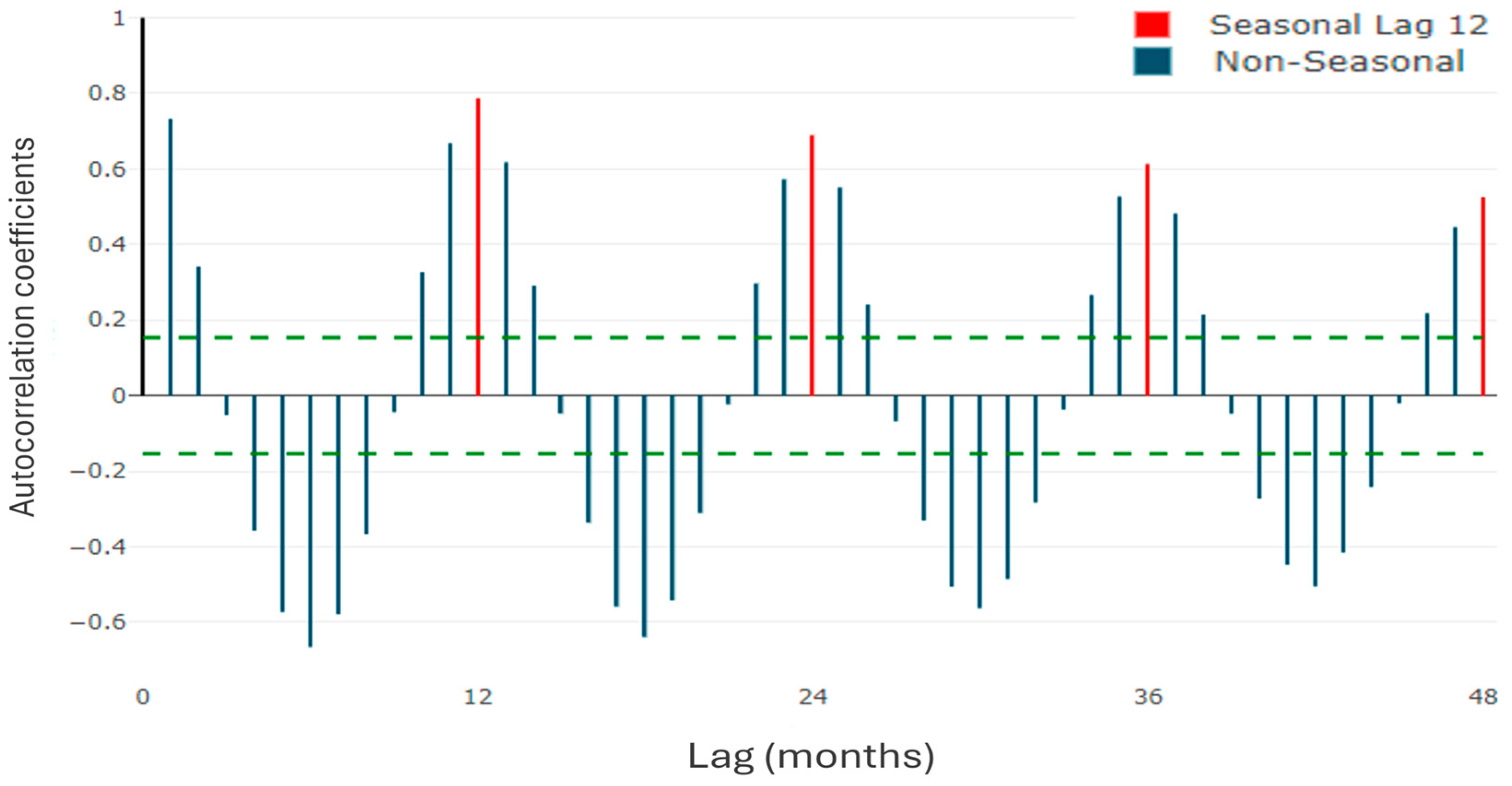
Figure 5 is presented below, showing the Autocorrelation Function (ACF) plot applied to the time series under study. This plot aims to evaluate the internal dependence of the series at different lags, allowing the identification of both seasonal and non-seasonal patterns—key information for the selection and validation of forecasting models.

The Autocorrelation Function (Figure 5) plot reveals marked seasonality in the time series, evidenced by significant peaks at lags 12, 24, 36, and 48 that exceed the confidence bounds. These lags, highlighted in red, indicate strong periodic dependence, suggesting that the series exhibits recurring behavior every 12 time units. In contrast, the non-seasonal lags show weaker and mostly insignificant autocorrelations. This pattern is characteristic of time series that require a seasonal component in the modeling process, such as SARIMA, to adequately capture the underlying temporal structure.

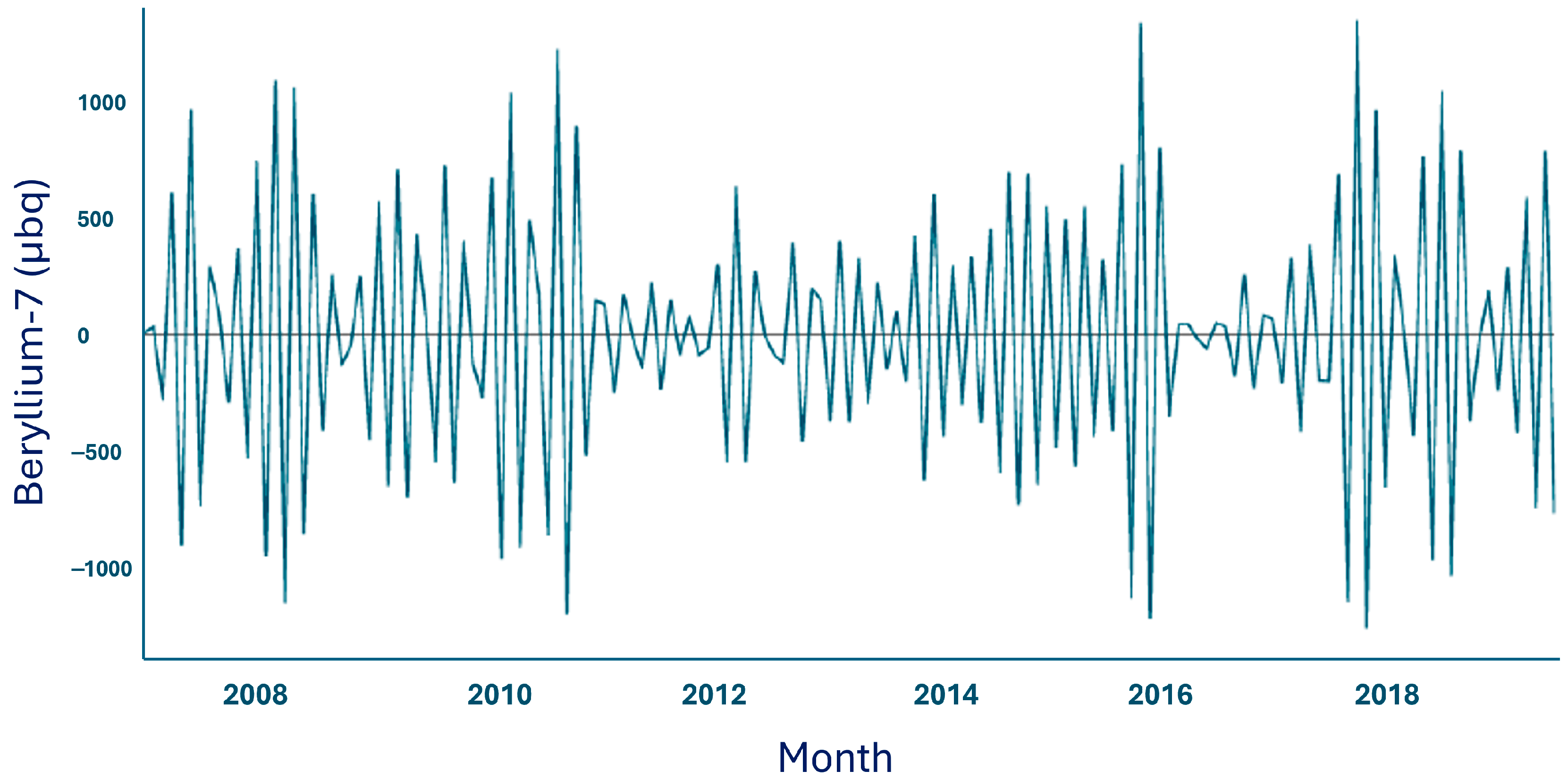
Continuing with the time series analysis, no differencing is required for the regular component. Differencing will be applied only to the seasonal component, as the correlogram shows a clear seasonal pattern in the series. A lag-12 differencing is performed to attempt to remove the seasonal pattern from the series and ultimately achieve what would be a white noise structure (Figure 6).

Figure 6 shows the series after first-order differencing, indicating the absence of a trend and a structure resembling white noise.

The time series was decomposed using a classical additive model, which separates the observed ⁷Be concentration data into three components: trend, seasonality, and residual. The first step involved identifying the trend by smoothing the data with a 12-month moving average, corresponding to the monthly resolution of the dataset. This trend component was then subtracted from the original series (Time Series—Trend).

Next, the seasonal component was estimated to capture recurring patterns within each year. This was done by averaging the values for each calendar month across all years of the study period—for example, calculating the mean of all January values, all February values, and so on. These monthly averages were then repeated throughout the entire time series to construct the seasonal pattern.

Finally, the residual component was obtained by removing both the trend and seasonal components from the original series, thereby representing short-term fluctuations and variations not explained by the other components. This procedure yielded the residual series, which behaves similarly to white noise, as illustrated in Figure 6.

To assess the stationarity of the time series, the Augmented Dickey–Fuller (ADF) test was applied. The null hypothesis (Ho) of this test posits the existence of a unit root, which would indicate that the series is non-stationary. The results showed a p-value of 0.01 and a Dickey–Fuller test statistic of −10.09. Since the p-value is less than the significance level of 0.05, the null hypothesis is rejected, confirming that the data are stationary. This finding is important, as stationarity prevents trends from biasing the data and ensures the accuracy of forecasts based on ARIMA models.

To assess whether the variance of ⁷Be activity concentrations is constant across different periods, Levene’s test for homogeneity of variances was applied. The hypotheses were defined as follows: H₀: The variances across periods are equal. H₁: At least one period has a different variance. The test results were as follows: F = 1.018, with 11 and 138 degrees of freedom for the numerator and denominator, respectively, and a p-value of 0.4338. At a 5% significance level, the p-value is greater than 0.05, indicating that the null hypothesis cannot be rejected. Therefore, the variance of ⁷Be activity concentrations can be considered homogeneous across periods, supporting the assumption of stationarity in variance.

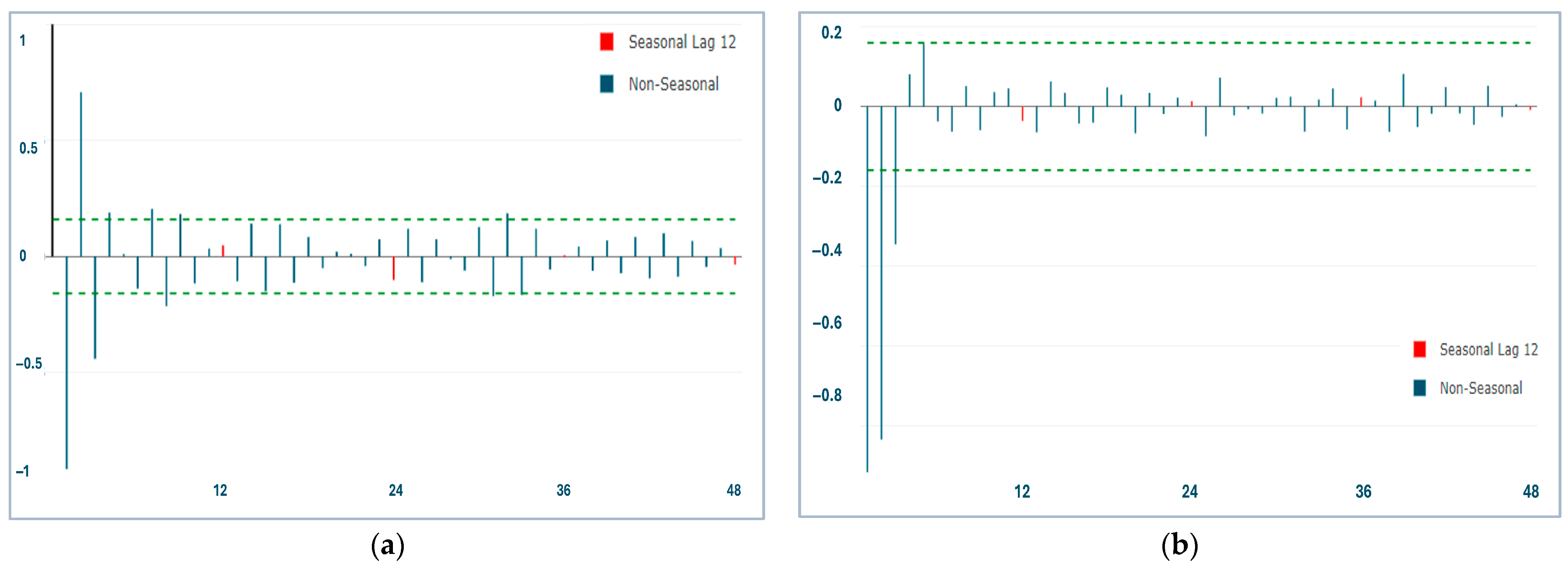
To determine the SARIMA (p,d,q) × (P,D,Q) models, it is necessary to study the plots of the autocorrelation function (ACF) and the partial autocorrelation function (PACF) of the differenced series. Figure 7 shows both plots, and the next step is to identify the autoregressive (p) and moving average (q) terms in the regular and seasonal components of a SARIMA (p,d,q) × (P,D,Q) model.

After applying seasonal differencing with lag 12, Figure 7 shows the reduction in the seasonal pattern and the approximation to white noise.

Based on the analysis of the correlograms, the following SARIMA models were selected to fit the ⁷Be time series (

Table 3. AIC values and Ljung–Box test results for the proposed SARIMA models.

Model	AIC	Ljung—Box p-Value
SARIMA (1,0,1) (0,1,0)	2354.6	0.0002
SARIMA (2,0,1) (0,1,0)	2356.4	0.0002
SARIMA (2,0,2) (0,1,0)	2347.6	0.0008
SARIMA (2,0,3) (0,1,0)	2344.6	0.0042
SARIMA (1,0,1) (1,1,0)	2329.6	0.0298
SARIMA (2,0,1) (1,1,0)	2331.6	0.0231
SARIMA (2,0,1) (2,1,0)	2321.7	0.3411
SARIMA (2,0,2) (2,1,0)	2321.7	0.5680
SARIMA (2,0,2) (2,1,1)	2311.5	0.6785
SARIMA (2,0,2) (2,1,2)	2313.6	0.6750

), which presents the proposed models along with their AIC values and Ljung–Box test results.

Table 4. Error measures of the proposed models.

Model	ME	RMSE	MAE	MPE	MAPE	MASE
SARIMA (1,0,1) (0,1,0)	558.51	756.72	634.13	18.37	20.24	1.31
SARIMA (2,0,1) (0,1,0)	567.88	759.08	630.87	18.62	20.18	1.30
SARIMA (2,0,2) (0,1,0)	568.88	732.66	617.10	18.09	19.28	1.27
SARIMA (2,0,3) (0,1,0)	533.48	714.12	559.64	16.44	17.09	1.15
SARIMA (1,0,1) (1,1,0)	482.85	662.92	482.85	16.83	16.83	1.00
SARIMA (2,0,1) (1,1,0)	492.57	668.10	492.57	17.13	17.13	1.02
SARIMA (2,0,1) (2,1,0)	375.88	591.85	397.91	13.06	14.05	0.82
SARIMA (2,0,2) (2,1,0)	388.67	589.98	426.59	12.09	14.46	0.88
SARIMA (2,0,2) (2,1,1)	284.88	614.73	467.88	7.74	18.69	0.96
SARIMA (2,0,2) (2,1,2)	281.58	616.17	474.12	7.52	18.94	0.98

ME: Mean Error; RMSE: Root Mean Squared Error; MAE: Mean Absolute Error; MPE: Mean Percentage Error; MAPE: Mean Absolute Percentage Error; MASE: Mean Absolute Scaled Error.

shows the proposed models and their corresponding performance metrics.

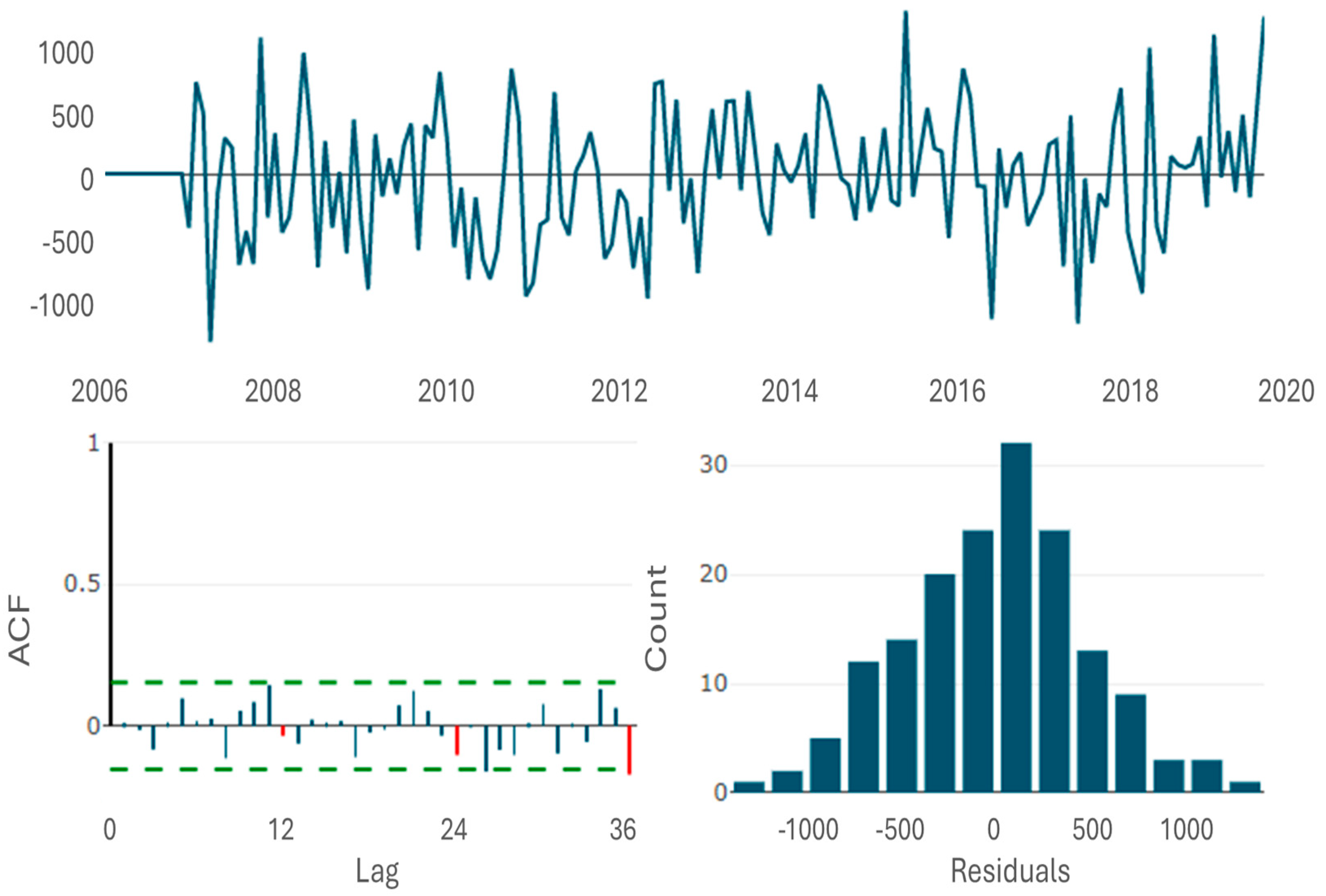
According to the error measures shown in Table 4, the SARIMA (2,0,2) (2,1,2) model has the lowest ME and the lowest MPE; the SARIMA (2,0,2) (2,1,0) model has the lowest RMSE; and the SARIMA (2,0,1) (2,1,0) model has the lowest MAE, MAPE, and MASE. This last model also ranked third in terms of AIC and yielded a p-value > 0.05 in the Ljung–Box test (Table 3). In addition, the ACF of the residuals for this model shows a white noise structure, while the histogram confirms the normality of the data (Figure 8).

Figure 8 shows that the residual time series exhibits no discernible trend. The autocorrelation function (ACF) suggests that the residuals behave as white noise, and the histogram indicates an approximately normal distribution.

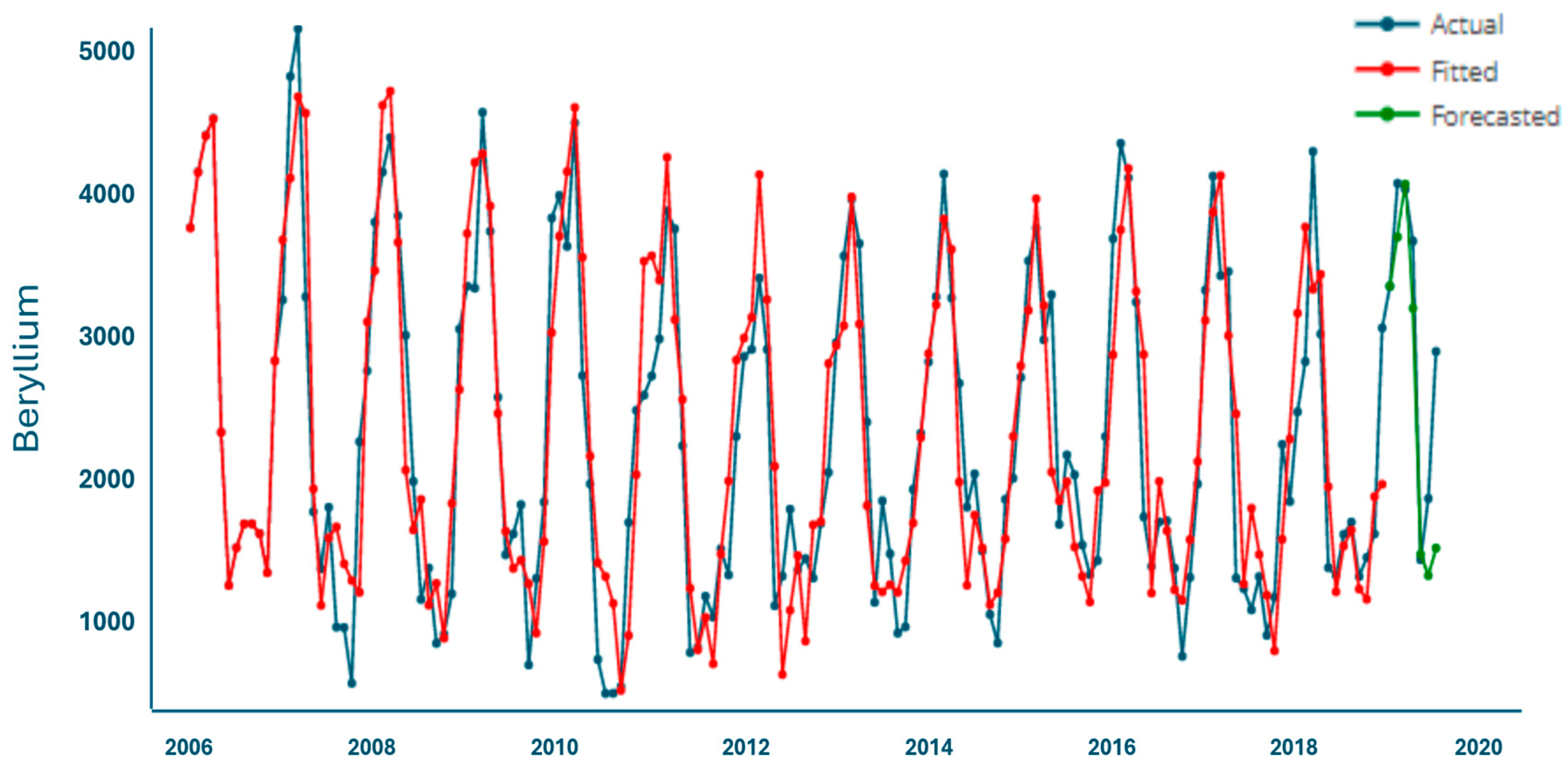
Figure 9 shows the model fit to the actual data and the forecast obtained in comparison with the observed values.

As shown in Figure 9, the model fit exhibited a high degree of concordance with the observed values, as evidenced by the overlap between the fitted and actual series. The inclusion of autoregressive and moving average terms with an annual periodicity (12 months) allowed for an adequate representation of the seasonal component.

Table 5. Observed and predicted values from the selected model with confidence intervals.

Month	Actual	Forecasted	95% CI Lower	95% CI Upper
January-2019	3382.27	3385.79	2394.24	4377.35
February-2019	4091.31	3722.01	2686.62	4757.41
March-2019	4048.48	4084.72	3044.73	5124.72
April-2019	3694.41	3233.51	2193.13	4273.88
May-2019	1507.94	1545.25	504.83	2585.67
June-2019	1927.56	1398.96	358.53	2439.38
July-2019	2937.00	1587.54	547.12	2627.96

presents the forecasted values for the first six months of 2019, along with a comparison against the actual values of the time series.

Table 5 shows that the forecasting model reasonably captures the monthly concentrations of beryllium-7 during the first months of 2019, with slight deviations in February and April, where the predicted values underestimated or overestimated the actual data. Most observations fall within the 95% confidence interval, indicating that the model is reliable. However, in May and June, the intervals are wider, reflecting greater uncertainty during periods with lower concentrations.

Table 6. Monthly forecast and confidence intervals from the selected model (Aug–Dec 2019).

Month	Forecasted	95% CI Lower	95% CI Upper
August 2019	2121.22	1126.66	3115.77
September 2019	1477.46	435.67	2519.24
October 2019	1293.97	244.97	2342.97
November 2019	1756.08	706.58	2805.59
December 2019	2483.60	1433.96	3533.23

and Figure 10 present the time series for the last five months of 2019, obtained using the selected model.

Figure 10 shows the five-month forecast of beryllium-7 concentration. The model suggests an initial increase, followed by a decrease and a slight rebound. Although the confidence intervals widen over time, the predictions remain within the historical range, indicating that the model adequately captures short-term fluctuations.

4. Discussion and Conclusions

The construction of the SARIMA model involved a meticulous process of parameter selection, fitting, and validation, guided by a rigorous analytical approach. As part of this procedure, the autocorrelation structure of the time series was examined, differencing was applied to remove seasonality, and the orders (p, d, q) for the regular component and (P, D, Q) for the seasonal component were determined. Based on the analysis of correlograms, various model configurations were evaluated using performance metrics such as RMSE, MSE, AMAPE, and MAPE, which enabled the selection of a model that effectively captured the dynamics of the series under study. Residual analysis during the validation stage confirmed the model’s suitability for forecasting, a result consistent with the findings of Bas et al. [45], who also demonstrated the predictive capability of the SARIMA model based on residual behavior

In this study, the selected SARIMA (2,0,1) (2,1,0) model not only allows for accurate forecasting but also provides deeper insight into the temporal behavior of suspended particles in the Panamanian atmosphere. The validity of SARIMA as a predictive tool is supported by previous studies such as that of Bas et al. [46], who applied this approach to model ⁷Be concentrations in Spain, using error metrics to assess forecast accuracy. Similarly, the consistency of the seasonal patterns identified aligns with the findings of Chham et al. [47], who reported seasonal patterns in nine out of ten Spanish regions, suggesting that ⁷Be seasonality is a recurrent feature across different geographic contexts.

Conversely, Bianchi et al. [48] observed that maximum and minimum values do not follow a consistent pattern across years, and that variance exhibits significant fluctuations. These results contrast with the findings of our study, which identified greater interannual regularity and more stable variance. According to the authors, this dynamic suggests that although a recurrent pattern exists, its intensity and shape are modulated by meteorological factors such as atmospheric pressure and temperature, potentially linked to changes in atmospheric dynamics or aerosol transport processes [49]—an aspect that warrants further exploration in future studies.

The results of the present study also align with those of Alegría et al. [15], who reported significant seasonal and monthly variation in beryllium concentrations, reinforcing the relevance of the seasonal component in ⁷Be dynamics.

This concordance between previous studies and the current analysis validates the use of the SARIMA model as both an explanatory and predictive tool for ⁷Be, while also highlighting the importance of incorporating meteorological variables [50] to enrich the understanding of the factors that modulate its behavior in future time series analyses. Finally, comparing the behavior of ⁷Be with that of other environmentally relevant particles could significantly deepen our understanding of the processes that govern its presence and variability in the atmosphere.

References

1. Ren, X.; Luke, W.T.; Kelley, P.; Cohen, M.; Ngan, F.; Artz, R.; Walker, J.; Brooks, S.; Moore, C.; Swartzendruber, P.; et al. Mercury Speciation at a Coastal Site in the Northern Gulf of Mexico: Results from the Grand Bay Intensive Studies in Summer 2010 and Spring 2011. Atmosphere 2014, 5, 230–251. [Google Scholar] [CrossRef]
2. Janković, M.M.; Todorović, D.J.; Nikolić, J.D.; Rajačić, M.M.; Pantelić, G.K.; Sarap, N.B. Aktivnost Berilijuma-7 i Olova-210 u Prizemnom Sloju Atmosfere u Srbiji. Hem. Ind. 2014, 68, 83–88. [Google Scholar] [CrossRef]
3. Lal, D.; Peters, D. Cosmic Ray Produced Radioactivity on the Earth. In Kosmische Strahlung II/cosmic rays II; Springer: Berlin/Heidelberg, Germany, 1967; pp. 551–612. [Google Scholar]
4. Kaste, J.M.; Norton, S.A. Environmental Chemistry of Beryllium-7. Rev. Miner. Geochem. 2002, 50, 271–289. [Google Scholar] [CrossRef]
5. Yoshimori, M.; Hirayama, H. Production of 7Be Nuclei in the Earth’s Upper Atmosphere from Galactic Cosmic Rays and Solar Energetic Particles. In Proceedings of the 28th International Cosmic Ray Conference, Tsukuba, Japan, 31 July–7 August 2003. [Google Scholar]
6. Papastefanou, C.; Ioannidou, A. Aerodynamic Size Association of 7Be in Ambient Aerosols. J. Environ. Radioact. 1995, 26, 273–282. [Google Scholar] [CrossRef]
7. Lal, D.; Malhotra, P.K.; Peters, B. On the Production of Radioisotopes in the Atmosphere by Cosmic Radiation and Their Application to Meteorology. Atmos. Terr. Phys. 1958, 12, 306–328. [Google Scholar] [CrossRef]
8. Bhandari, N.; Lal, D. Rama Vertical Structure of the Troposphere as Revealed by Radioactive Tracer Studies. J. Geophys. Res. 1970, 75, 2974–2980. [Google Scholar] [CrossRef]
9. Cannizzaro, F.; Greco, G.; Raneli, M.; Spitale, M.C.; Tomarchio, E. Concentration Measurements of 7Be at Ground Level Air at Palermo, Italy—Comparison with Solar Activity over a Period of 21 Years. J. Env. Radioact. 2004, 72, 259–271. [Google Scholar] [CrossRef] [PubMed]
10. Usoskin, I.G.; Bazilevskaya, G.A.; Kovaltsov, G.A. Solar Modulation Parameter for Cosmic Rays since 1936 Reconstructed from Ground-Based Neutron Monitors and Ionization Chambers. J. Geophys. Res. Space Phys. 2011, 116, A02104. [Google Scholar] [CrossRef]
11. Nandy, D.; Martens, P.C.H.; Obridko, V.; Dash, S.; Georgieva, K. Solar Evolution and Extrema: Current State of Understanding of Long-Term Solar Variability and Its Planetary Impacts. Prog. Earth Planet. Sci. 2021, 8, 40. [Google Scholar] [CrossRef]
12. Stozhkov, Y.; Makhmutov, V.; Svirzhevsky, N. About Cosmic Ray Modulation in the Heliosphere. Universe 2022, 8, 558. [Google Scholar] [CrossRef]
13. Ioannidou, A.; Paatero, J. Activity Size Distribution and Residence Time of 7Be Aerosols in the Arctic Atmosphere. Atmos. Env. 2014, 88, 99–106. [Google Scholar] [CrossRef]
14. Landis, J.D.; Feng, X.; Kaste, J.M.; Renshaw, C. Patterns and Processes in Aerosol Bulk Deposition: Insights from a 9-Year Study of 7Be, 210Pb, Sulfate and Major/Trace Elements. Authorea Prepr. 2022. [Google Scholar] [CrossRef]
15. Alegría, N.; Hernández-Ceballos, M.Á.; Herranz, M.; Idoeta, R.; Legarda, F. Meteorological Factors Controlling 7Be Activity Concentrations in the Atmospheric Surface Layer in Northern Spain. Atmosphere 2020, 11, 1340. [Google Scholar] [CrossRef]
16. You, C.F.; Lee, T.; Yi, Y.H. The Partition of Be between Soil and Water. Chem. Geol. 1989, 77, 105–118. [Google Scholar] [CrossRef]
17. Ryken, N.; Al-Barri, B.; Blake, W.; Taylor, A. Rapid and Irreversible Sorption Behavior of 7Be Assessed to Evaluate Its Use as a Catchment Sediment Tracer. J. Env. Radioact. 2018, 182, 108–116. [Google Scholar] [CrossRef]
18. Pérez, O.C.; Fernández, B.G. Trazadores Atmosféricos BE-7, K-40 Y PB-210 en la Ciudad de Panamá. Scientia 2019, 29, 44–67. [Google Scholar]
19. Benchrif, A.; Khalfaoui, O.; Baghdad, B.; Jung, C.H.; Tahri, M.; Baghdad, B.; Bounakhla, M.; Cachier, H. Aerosols in Northern Morocco (Part 4): Seasonal Chemical Signatures of PM 2.5 and PM 10. Atmosphere 2025, 16, 982. [Google Scholar] [CrossRef]
20. Olivares-Salazar, S.E.; Bahreini, R.; Lin, Y.H.; Castro, T.; Alvarez-Ospina, H.; Salcedo, D. Aerosol Composition in a Semi-Urban Environment in Central Mexico: Influence of Local and Regional Processes on Overall Composition and First Quantification of Nitroaromatics. Atmosphere 2025, 16, 827. [Google Scholar] [CrossRef]
21. Guo, Q.; He, Z.; Wang, Z. The Characteristics of Air Quality Changes in Hohhot City in China and Their Relationship with Meteorological and Socio-Economic Factors. Aerosol Air Qual. Res. 2024, 24, 230274. [Google Scholar] [CrossRef]
22. Papastefanou, C. Beryllium-7 Aerosols in Ambient Air. Aerosol Air Qual. Res. 2009, 9, 187–197. [Google Scholar] [CrossRef]
23. Johnson, W.B.; Viezee, W. Stratospheric Ozone in the Lower Troposphere—I. Presentation and Interpretation of Aircraft Measurements. Atmos. Env. 1981, 15, 1309–1323. [Google Scholar] [CrossRef]
24. Feely, H.; Larsen, R.; Sanderson, C.G. Factors That Cause Seasonal Variations in Beryllium-7 Concentrations in Surface Air. J. Env. Radioact. 1989, 9, 223–249. [Google Scholar] [CrossRef]
25. Kremenchutskii, D.A. Influence of Precipitation on the Daily Beryllium-7 (7Be) Activity Concentration in the Atmospheric Surface Layer. J. Env. Radioact. 2021, 237, 106722. [Google Scholar] [CrossRef]
26. Wallbrink, P.J.; Murray, A.S. Use of Fallout Radionuclides as Indicators of Erosion Processes. Hydrol. Process 1993, 7, 297–304. [Google Scholar] [CrossRef]
27. Wallbrink, P.J.; Murray, A.S. Distribution and Variability of 7Be in Soils Under Different Surface Cover Conditions and Its Potential for Describing Soil Redistribution Processes. Water Resour. Res. 1996, 32, 467–476. [Google Scholar] [CrossRef]
28. Blake, W.; Walling, D.; He, Q. Fallout Beryllium-7 as a Tracer in Soil Erosion Investigations. Elsevier 1999, 51, 599–605. [Google Scholar] [CrossRef]
29. Schuller, P.; Iroumé, A.; Walling, D.E.; Mancilla, H.B.; Castillo, A.; Trumper, R.E. Use of Beryllium-7 to Document Soil Redistribution Following Forest Harvest Operations. J. Environ. Qual. 2006, 35, 1756–1763. [Google Scholar] [CrossRef]
30. Yang, M.Y.; Walling, D.E.; Tian, J.L. Partitioning the Contributions of Sheet and Rill Erosion Using Beryllium-7 and Cesium-137. Soil. Sci. Soc. Am. J. 2006, 70, 1579–1590. [Google Scholar] [CrossRef]
31. Saari, H.; Schmidt, S.; Castaing, P.; Blanc, G.; Sautour, B.; Masson, O.; Cochran, J.K. The Particulate 7Be/210Pbxs and 234Th/210Pbxs Activity Ratios as Tracers for Tidal-to-Seasonal Particle Dynamics in the Gironde Estuary (France): Implications for the Budget of Particle-Associated Contaminants. Sci. Total Environ. 2010, 408, 4784–4794. [Google Scholar] [CrossRef] [PubMed]
32. Li, Z.; Lu, Y.; Nie, X.; Huang, B.; Ma, W.; Liu, C.; Xiao, H. Variability of Beryllium-7 and Its Potential for Documenting Soil and Soil Organic Carbon Redistribution by Erosion. Wiley Online Libr. 2016, 80, 693–703. [Google Scholar] [CrossRef]
33. Martınez-Casasnovas, J.; Ramos, M.; Geoderma, M.R.-D. Soil Erosion Caused by Extreme Rainfall Events: Mapping and Quantification in Agricultural Plots from Very Detailed Digital Elevation Models. Geoderma 2002, 105, 125–140. [Google Scholar] [CrossRef]
34. Fernández, B.; Juri Ayub, J.; Valladares, D.; Pérez, O.; Tejedor-Flores, N.; Esquivel-López, A. 7Be Atmospheric Concentration in Panama City: Influence of Climatic Conditions and Atmospheric Recovery Process. Isot. Env. Health Stud. 2025, 61, 351–370. [Google Scholar] [CrossRef]
35. Box, G.; Jenkins, G.M. Analysis: Forecasting and Control; Holden-Day: San Francisco, CA, USA, 1976. [Google Scholar]
36. Ryabko, D. Asymptotic Nonparametric Statistical Analysis of Stationary Time Series; Springer International Publishing: Cham, Switzerland, 2019. [Google Scholar]
37. Chintalapudi, N.; Battineni, G.; Amenta, F. COVID-19 Virus Outbreak Forecasting of Registered and Recovered Cases after Sixty Day Lockdown in Italy: A Data Driven Model Approach. J. Microbiol. Immunol. Infect. 2020, 53, 396–403. [Google Scholar] [CrossRef]
38. Noor, T.H.; Almars, A.M.; Alwateer, M.; Almaliki, M.; Gad, I.; Atlam, E.S. SARIMA: A Seasonal Autoregressive Integrated Moving Average Model for Crime Analysis in Saudi Arabia. Electronics 2022, 11, 3986. [Google Scholar] [CrossRef]
39. RStudio: Integrated Development for R, Version 4.2.1, [Computer Software]. RStudio PBC: Boston, MA, USA, 2020.
40. Armstrong, J.S.; Collopy, F. Error Measures for Generalizing about Forecasting Methods: Empirical Comparisons. Int. J. Forecast. 1992, 8, 69–80. [Google Scholar] [CrossRef]
41. St-Aubin, P.; Agard, B. Precision and Reliability of Forecasts Performance Metrics. Forecasting 2022, 4, 882–903. [Google Scholar] [CrossRef]
42. Jierula, A.; Wang, S.; Oh, T.M.; Wang, P. Study on Accuracy Metrics for Evaluating the Predictions of Damage Locations in Deep Piles Using Artificial Neural Networks with Acoustic Emission Data. Appl. Sci. 2021, 11, 2314. [Google Scholar] [CrossRef]
43. Yadav, B.K.; Srivastava, S.K.; Arasu, P.T.; Singh, P. Time Series Modeling of Tuberculosis Cases in India from 2017 to 2022 Based on the SARIMA-NNAR Hybrid Model. Can. J. Infect. Dis. Med. Microbiol. 2023, 2023, 5934552. [Google Scholar] [CrossRef] [PubMed]
44. Cubilla-Montilla, M.; Ramírez, A.; Escudero, W.; Cruz, C. Analyzing and Forecasting Vessel Traffic Through the Panama Canal: A Comparative Study. Appl. Sci. 2025, 15, 8389. [Google Scholar] [CrossRef]
45. Bas, M.d.C.; Ortiz, J.; Ballesteros, L.; Martorell, S. Evaluation of a Multiple Linear Regression Model and SARIMA Model in Forecasting 7Be Air Concentrations. Chemosphere 2017, 177, 326–333. [Google Scholar] [CrossRef]
46. Bas, M.d.C.; Ortiz, J.; Ballesteros, L.; Martorell, S. Forecasting 7BE Concentrations in Surface Air Using Time Series Analysis. Atmos. Env. 2017, 155, 154–161. [Google Scholar] [CrossRef]
47. Chham, E.; Piñero-García, F.; Brattich, E.; El Bardouni, T.; Ferro-García, M.A. 7Be Spatial and Temporal Pattern in Southwest of Europe (Spain): Evaluation of a Predictive Model. Chemosphere 2018, 205, 194–202. [Google Scholar] [CrossRef] [PubMed]
48. Bianchi, S.; Longo, A.; Plastino, W. A New Methodological Approach for Worldwide Beryllium-7 Time Series Analysis. Phys. A Stat. Mech. Its Appl. 2018, 501, 377–387. [Google Scholar] [CrossRef]
49. Bianchi, S.; Plastino, W.; Brattich, E.; Djurdjevic, V.; Longo, A.; Hernández-Ceballos, M.A.; Sarvan, D.; Ajtić, J. Analysis of Trends, Periodicities, and Correlations in the Beryllium-7 Time Series in Northern Europe. Appl. Radiat. Isot. 2019, 148, 160–167. [Google Scholar] [CrossRef] [PubMed]
50. Houali, A.; Azahra, M.; El Bardouni, T.; Ferro García, M.A.; Piňero García, F.; Chham, E. Impact of the Meteorological Parameters on the Behaviour of 7Be at Ground Level in Tetouan City, Morocco from June 2015 to February 2017. J. Radioanal. Nucl. Chem. 2019, 322, 271–280. [Google Scholar] [CrossRef]
Figure 1. Box–Jenkins methodology.
Atmosphere 16 01104 g001
Figure 2. Time series of 7Be from 2006 to 2019.
Atmosphere 16 01104 g002
Figure 3. Additive decomposition of the series.
Atmosphere 16 01104 g003
Figure 4. Box plot and scatter plot of 7Be concentrations.
Atmosphere 16 01104 g004
Figure 5. Autocorrelation function (ACF) plot of 7Be concentration.
Atmosphere 16 01104 g005
Figure 6. Seasonal decomposition of the 7Be time series.
Atmosphere 16 01104 g006
Figure 7. (a) ACF plot of 7Be concentration; (b) PACF plot of 7Be concentration.
Atmosphere 16 01104 g007
Figure 8. Residual diagnostics of the ARIMA (2,0,1) (2,1,0) model.
Atmosphere 16 01104 g008
Figure 9. Actual 7Be concentration vs. forecasted 7Be concentration.
Atmosphere 16 01104 g009
Figure 10. Forecast of 7Be concentrations for the last five months of 2019 with confidence intervals.
Atmosphere 16 01104 g010