Improved Daytime Cloud Detection Algorithm in FY-4A’s Advanced Geostationary Radiation Imager

Abstract

Cloud detection is an indispensable step in satellite remote sensing of cloud properties and objects under the influence of cloud occlusion. Nevertheless, interfering targets such as snow and haze pollution are easily misjudged as clouds for most of the current algorithms. Hence, a robust cloud detection algorithm is urgently needed, especially for regions with high latitudes or severe air pollution. This paper demonstrated that the passive satellite detector Advanced Geosynchronous Radiation Imager (AGRI) onboard the FY-4A satellite has a great possibility to misjudge the dense aerosols in haze pollution as clouds during the daytime, and constructed an algorithm based on the spectral information of the AGRI’s 14 bands with a concise and high-speed calculation. This study adjusted the previously proposed cloud mask rectification algorithm of Moderate-Resolution Imaging Spectroradiometer (MODIS), rectified the MODIS cloud detection result, and used it as the accurate cloud mask data. The algorithm was constructed based on adjusted Fisher discrimination analysis (AFDA) and spectral spatial variability (SSV) methods over four different underlying surfaces (land, desert, snow, and water) and two seasons (summer and winter). This algorithm divides the identification into two steps to screen the confident cloud clusters and broken clouds, which are not easy to recognize, respectively. In the first step, channels with obvious differences in cloudy and cloud-free areas were selected, and AFDA was utilized to build a weighted sum formula across the normalized spectral data of the selected bands. This step transforms the traditional dynamic-threshold test on multiple bands into a simple test of the calculated summation value. In the second step, SSV was used to capture the broken clouds by calculating the standard deviation (STD) of spectra in every 3 × 3-pixel window to quantify the spectral homogeneity within a small scale. To assess the algorithm’s spatial and temporal generalizability, two evaluations were conducted: one examining four key regions and another assessing three different moments on a certain day in East China. The results showed that the algorithm has an excellent accuracy across four different underlying surfaces, insusceptible to the main interferences such as haze and snow, and shows a strong detection capability for broken clouds. This algorithm enables widespread application to different regions and times of day, with a low calculation complexity, indicating that a new method satisfying the requirements of fast and robust cloud detection can be achieved.

1. Introduction

An accurate cloud detection algorithm is essential for meteorological satellite observation, not only because it is the basis of cloud property acquisition, but also due to the fact that cloud occlusion is an inescapable obstacle to satellite atmospheric and ground surface observations. Cloud detection accuracy is crucially important to a series of satellite products. Previous studies demonstrated great difficulty in cloud detection of seriously polluted regions for onboard passive remote sensing because the dense aerosols strongly influence the incoming and outgoing radiation [1,2]. A suitable cloud detection algorithm is indispensable to passive cloud remote sensing in haze regions.

The current algorithms include the traditional and intelligent methods. The threshold algorithm is one of the most widely used traditional methods in passive detectors, such as Moderate-Resolution Imaging Spectroradiometer (MODIS) [3,4] and Advanced Very-High-Resolution Radiometer (AVHRR) [5]. Nevertheless, this approach turned out to be susceptible to surface and atmospheric conditions. As indicated, urban aerosol causes a significantly overestimated cloud fraction for AVHRR [6]. The MODIS misjudges large areas of cloud-free haze regions as cloudy in East China’s winter, for the dense aerosols interfere with the satellite-received radiation and reduce the contrast between cloudy and cloud-free regions [2,7,8]. Error in cloud detection causes invalid cloud property retrievals, introducing obvious bias to regional research [8]. A similar phenomenon appeared in the AVHRR, with the satellite-observed cloud fraction being substantially bigger than the surface observation under the influence of urban aerosol.

Regarding the inaccuracy of the mainstream passive detectors’ cloud detection, multiple intelligent algorithms have been proposed to reduce these interfering factors and find a robust algorithm. The most general approach is to utilize machine learning. This approach trains the model with the prior spectral library and then recognizes clouds using the well-trained model. The supervised machine learning algorithms include convolutional neural networks [9,10], random forest [11,12], randomized tree [13,14], and support vector machine [15,16,17]. Compared with the traditional methods, machine learning attained a better performance in cloud detection, and part of them apply to diverse sensors [10,17].

Moreover, there are also some intelligent approaches constructed based on statistical or modeling analysis. The haze optimized transformation (HOT) algorithm was developed to overcome the effect of haze pollution. This algorithm constructs a multi-dimensional visible-band space with features including a high correlation of reflectance from diverse underlying surfaces and differentiated enough responses of the bands to haze pollution. The reflection from the surface forms a clear line vector, and the perpendicular distance reflects the atmospherically induced reflection variance [18,19]. This method is also applied as a part of other cloud detection algorithms [20], and Huang et al. [21] put forward an automated masking algorithm with a similar idea to the clean line.

Another intelligent approach is automatic cloud cover assessment (ACCA), developed by the LandSat Project Science Office at NASA’s Goddard Space Flight Center (GSFC) [22]. It first conducts preliminary cloud detection to determine the confident cloud-free pixels and extracts the features, such as the spectral, statistical, and textural features of each pixel. Then, secondary recognition employing the extracted features is performed further to classify the ambiguous pixels in the first step. This method has an auto-detect function for cloud detection without extra references or manual intervention. Multiple methods are proven to generate a cloud/clear weighting in the two steps. The first proposed one is a threshold test usually used in the first step, including tests about spectra and the corresponding indices [23,24,25]. As the spectra of thin or broken clouds are usually contaminated by land-surface-reflected radiation, the second method, fuzzy cluster analysis, including k-means [25] and c-means clustering [26,27], has been proven to overcome the ambiguity in thin cloud recognition of ACCA. Machine learning is also used to resolve this issue. Ma et al. [28] applied a convolutional neural network in spectral information capture and performed well, including in thin and broken clouds. As ACCA distinguishes clouds by referring to cloud-free pixels in the detection image, non-cloud areas are a prerequisite for accurate detection. To avoid bias in the cloud-filled images, previous studies proved a multi-temporal method utilizing the images in a time series [12,25]. Nevertheless, this method is still inapplicable to images of continuously overcast areas.

FengYun-4A (FY-4A) is the first launched satellite in the new generation of Chinese FY-4 series geostationary satellites, which was lifted off on 11 December 2016. Four payloads are equipped on FY-4A, which are the Advanced Geosynchronous Radiation Imager (AGRI), the Geostationary Interferometric Infrared Sounder (GIIRS), the Lightning Mapping Imager (LMI), and the Space Environment Package (SEP), achieving continuous observations over most of the eastern hemisphere [29,30]. AGRI is a radiation imager used primarily in cloud image capture with 14 channels, nearly triple that of the pre-launched Stretched Visible and Infrared Spin Scan Radiometer-II (VISSR-II) on FengYun-2H. This detector provides the spectral data of visible, near-infrared, and infrared channels in the daytime, and infrared channels during the night, and its products include real-time situation of clouds, aerosols, moisture, and the land surface. However, the orbital altitude of a geostationary satellite (35,786 km) is much higher than that of a typical polar-orbit satellite, which inevitably influences the spatial resolution and accuracy [31].

As a passive remote-sensing detector, the cloud mask product of AGRI is obtained by the threshold evaluation algorithm, a physical rule-based method that relies on the empirical analysis of the spectral contrast between cloudy and cloud-free pixels, determining the thresholds to segment the clouds [29]. As many regions within and surrounding China have high haze incidences, the FY-4A cloud detection product in China area deserves a reliable evaluation, and a robust cloud detection algorithm with low computing cost is essential for its official operation.

In this study, all 14 spectra were utilized to build an algorithm suitable for the cloud detection of the passive detector AGRI in severely polluted regions. Since visible and near-infrared spectra are only available during daytime, this algorithm only focuses on daytime cloud detection. The construction used two methods with cost-efficient computing. The first one was a cloud detection rectification algorithm regarding the problem that MODIS misidentifies dense aerosol in haze regions as clouds, which was confirmed to be robust [7,8]. The algorithm mainly uses the adjusted Fisher classification method (AFDA), which generates a weighted sum formula with multiple apparent spectral parameters as the independent variable and a y-value as the dependent variable. A threshold test on the y-value can effectively eliminate the misidentified pixels of MODIS [7]. The second one is a spatial variability method that uses the threshold test on 3 × 3-STD (standard deviation of spectrums in every 3 × 3-pixel window) to distinguish broken clouds whose spectrums are more spatially heterogeneous than other targets [32].

This study made a detailed assessment of the AGRI cloud mask product and proved a new daytime cloud detection algorithm that combines AFDA and SSV. The algorithm was proven to be highly efficient and robust in cloud detection in China area.

2. Materials and Methods

2.1. Datasets

In this research, cloud products including AGRI/FY-4A, MODIS/Aqua, the Advanced Himawari Imager (AHI), true-color images of MODIS and AHI, the spectral products of MODIS and AGRI, and the vertical feature product (VFM) of CALIPSO, over China and surrounding areas (60–137° E, 3–55° N), were used in the assessment of AGRI cloud mask and to build the AGRI cloud detection algorithm.

AGRI/FY-4A has three scanning modes, including the whole-earth image from satellite, which is called full disk (once every 15 min), China area image (60–137° E, 3–55° N, once every 5 min), and target area image (once every 1 min) [31,33]. Compared with the detectors onboard the previous generations of FY satellites, AGRI has made significant progress in the spectral channels and spatial resolution, providing observations of 14 channels, which include 2 visible channels, 1 near-infrared channel, and 11 infrared channels. The spatial resolution is 500 m for the 0.64 μm band, 1 km for the 0.47 μm band and 0.83 μm bands, and 4 km for the rest of the infrared bands. Similar to MODIS [34], the AGRI cloud mask product separates each pixel into “cloud”, “probably cloud”, “probably clear”, and “clear”. Studies usually regard the first two categories as “cloudy” and the last two kinds as “cloud-free”.

MODIS is a passive detector onboard the Terra and Aqua satellites. Aqua is a sun-synchronous orbit satellite, passing a certain region twice a day at 01:30 and 13:30 local time (LT), respectively. This study used the daytime data of the level 2 daily 1 km product (MYD35_L2, Collection 6) and the corresponding rectified product [31], which have a spatial resolution of 1 km.

The Cloud–Aerosol Lidar with Orthogonal Polarization (CALIOP) is a polarization ratio-sensitive backscatter lidar with two wavelengths (532 nm and 1064 nm) on board CALIPSO satellite. VFM is a profile product containing the mask of cloud and aerosol at an along-track resolution of 333 m, vertical resolutions of 30 m below 8.2 km, and 60 m between 8.2 km and 20.2 km [35,36]. This study regards the profiles with clouds at any level as cloudy.

The AHI aboard Himawari-8 is a passive detector with 16 spectrums, ranging from visible to infrared bands, at high spatial resolutions. AHI provides a cloud detection product generated by a threshold algorithm with a hit rate of 0.85 in comparison with MODIS cloud mask product. It should be noted that the detection result of AHI is slightly higher than that of the MODIS, which means part of the cloud-free areas in MODIS detection is classified as cloudy by AHI. As Himawari-8 is a geostationary satellite, AHI can achieve round-the-clock monitoring and provide one satellite image every 10 min. Therefore, AHI cloud mask product was used to assess the AGRI cloud mask at different moments in one day.

2.2. Methodology

This study constructed a concise algorithm combining AFDA and SSV. AFDA builds one formula for each kind of underlying surface of summer and winter, which screens the confident cloud clusters. Then, the cloud-free regions were checked with SSV as a complementary recognition method for the broken clouds, including cellular clouds and edge clouds.

2.2.1. Adjusted Fisher Discriminant Analysis (AFDA)

AFDA is the method introduced in the study of Zhang et al. [7] and used as part of the cloud mask rectification algorithm. In this study, two sample sets, the cloudy group and cloud-free group, which were selected by the rectified MODIS/Terra and Aqua cloud mask result using the method proved by Zhang et al. [7], were collected as the input data. Fisher discriminant analysis was conducted on the spectral radiance values (the reflection of bands 1 to 6 and the brightness temperature of bands 7 to 14) of cloudy and cloud-free samples over 4 kinds of underlying surfaces (land, desert, snow, and water) and 2 seasons (summer and winter), constructing, in total, 8 weighted sum formulas formed as

$$y=\sum _{i=1}^6{c}_i{R}_i+\sum _{i=7}^{14}{c}_i{T}_i,$$

(1)

where R_i is the normalized reflection of band 1 to band 6, T_i is the normalized brightness temperature of bands 7 to 14, and c_i represents the weight coefficients. Clouds are recognized by a threshold test of the y-value, the weighted sum value. A threshold value y₀ is selected through a probability density analysis of the y-value for cloudy and cloud-free samples.

2.2.2. Spectral Spatial Variability (SSV)

SSV is an algorithm based on the threshold test of the standard deviation of spectra within each 3 × 3-pixel window. Previous studies found that this method is highly sensitive to broken clouds. In this paper, it was implemented to make up for the low sensitivity of AGRI caused by its high orbital altitude. In the cloud-free regions identified by AFDA, the SSV algorithm was used to perform an augmented discrimination on the 1 km spectral product to find out the broken clouds and the clouds on the edge of the cloud blocks via their inhomogeneous distribution of spectra.

The detailed flowchart of the algorithm is shown in Figure 1. The China area level 1 product, which is spectral data with a 4 km resolution, was used as the input of the AFDA formula. The underlying surface type was obtained from the cloud binary mask in the cloud mask product. Pixels with y-values smaller than the threshold y₀ would be recognized as cloudy, and the others would be used for SSV analysis with the 1 km L1 data. Pixels with STD values greater than the threshold STD₀ would be recognized as cloudy, and the others as clear.

3. Algorithm Construction

3.1. Multiple Detector Assessment

Under the assisted validation of the MODIS true-color image, the cloud mask product of multiple sensors was compared regarding the detection effect in two haze-polluted cases, which were 31 January 2020, and 27 December 2020, respectively. In the first case, most part of regions in East China (EC) were cloud-free, with only a small part of cloudy regions distributed in the southwest and East China Sea. A part of an ambiguous area, which could not be distinguished into clouds and snow from the true-color image, existed in Northeast China (NEC; Figure 2a). Although some uncertain clouds were detected in the eastern part, the cloud fraction of AHI was nearly consistent with the true-color image in most regions (Figure 2b). Large areas of misjudgment appeared in the cloud mask of MODIS and AGRI. MODIS recognized part of the cloud-free regions in the North China Plain as cloudy (Figure 2c), while the misrecognized region of AGRI was even larger than that of MODIS, including most of the North China Plain (NCP) and the Loess Plateau (Figure 2d). From Figure 2e, AGRI had a relatively consistent cloud top height with MODIS in most regions. The track of CALIPSO came across the NCP in the first case, in which regions between 25° N and 45° N were demonstrated to be cloud-free. Case 2 reflects a similar phenomenon, with the misclassified “clouds” of MODIS mainly distributed in the NCP and East China, and those of AGRI mainly distributed in the NCP. Figure 2j shows that the cloud top height of most of the misclassified “clouds” was not retrieved.

The accuracy of the AGRI cloud mask also showed a significant dependence on the time of day. As shown in Figure 3, the distribution of AGRI cloud mask showed a roughly opposite performance with AHI. The product of AHI was more error-prone before mid-morning and after mid-afternoon. At times earlier than 2:30 and later than 6:30, a certain part of misclassified “clouds” existed in the west region, which was probably caused by the big solar zenith angle. In contrast, the cloud mask of the AGRI was more accurate in the morning and dusk, and the misclassified “clouds” mainly existed in part of North China between 3:30 to 5:30 UTC.

3.2. Modification of MODIS Cloud Mask Rectification Algorithm

Selecting a set of reliable cloudy and cloud-free detection samples is necessary for the construction of a cloud detection algorithm. CALIPSO is a reliable detector for its sensitivity to thin clouds and resistance to aerosol effects. However, AGRI has a relatively short observation history and a large data size for one moment. Furthermore, CALIPSO only provides the profiles along the orbit as an active detector. All these limitations make it difficult to retrieve enough samples through data collocation with CALIPSO. In contrast, the passive detector MODIS can provide a complete coverage observation. Therefore, using the rectified MODIS cloud mask to decide the cloudy and cloud-free pixels is feasible if the rectification algorithm is reliable within the China area of the FY-4A product.

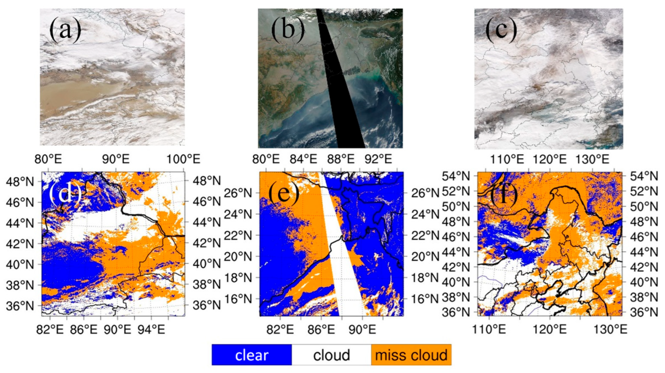
As the MODIS cloud detection rectification algorithm was built primarily based on the samples selected in East China, its applicability in other regions has not yet been verified. Assessment of the algorithm’s performance was conducted in order to ensure that the rectified MODIS cloud mask product is robust enough to act as the criterion of cloud detection. Except for East China, regions with strong interferences in the FY-4A’s field of view include the Taklimakan Desert, which is affected by dust, and North India, which has even more serious air pollution than East China. Moreover, the algorithm has no scheme regarding the snowy region, where the underlying snow would increase the difficulty of distinguishing between clouds and the underlying surface.

Figure 4 is the assessment result regarding the three regions. As can be seen, this algorithm had a relatively good performance in the western part of the Taklamakan Desert, with most of the misclassified “clouds” rectified (Figure 4c). However, a small number of the clouds in the southern part were eliminated by the algorithm. This can be verified by the AHI cloud detection result, in which the clouds eliminated in Figure 4c were determined as clouds. In contrast with the Taklamakan Desert, pollution in North India brought significant interference to MODIS cloud detection even after rectification. A large area with serious air pollution south of the Himalaya Mountains was misjudged as “cloudy” by MODIS, while the result after rectification still had a large deviation. A similar phenomenon existed over the southeast coastal water. A long stretch of brown regions, where it was hard to determine whether it was aerosols or silt, existed along the coast (Figure 4d). Both MODIS and AHI misjudged part of this area as cloudy, and the rectification was not effective. Assessments over the snowy region in North-East China also showed a high ambiguity in the cloud detection, both for MODIS and AHI (Figure 4e,f). Because it was difficult to discern clouds from the true-color image, assessment over snow was supplemented by the CALIPSO vertical feature mask, which is insusceptible to the underlying surface (Figure 4j). As can be seen, along the track in Figure 4g–i, the true clouds were basically fully covered by the cloud mask after rectification, while the misjudged “clouds” north of 52° N were not eliminated. AHI also had an overestimated cloud fraction over snow.

In order to obtain an accurate cloud detection indicator, a new Fisher discrimination was made based on the analysis of the samples selected in the whole FOV of FY-4A China area image (60–137° E, 3–55° N). The samples were selected by collocating the MODIS cloud mask and CALIPSO VFM data. As the orbits of CALIPSO and MODIS were not coincident in recent years, we used the data in the years 2015 to 2017. As research has demonstrated that MODIS observation is rarely affected by air pollution in summer, and the research area has no snow cover in summer, only the MODIS data in winter were rectified. The coefficients of AFDA and the thresholds of y are shown in

Table 1. AFDA function coefficients of MODIS in January and December.

	Land	Desert	Snow/Ice	Water
REF 3	1.299814	−1.08502	0.575017	2.017792
REF 9	−2.68352	0.146133	0.317414	−0.45535
REF 10	3.834834	3.898747	−0.21676	3.563714
REF 11	45.33824	−2.78985	−1.49741	−1.15359
REF 12	23.06156	7.064531	−0.42344	7.670586
BT 29	18.90707	33.7264	34.5497	−0.1916
BT 31	163.8991	216.9865	11.9891	144.5935
BT 32	−135.508	−209.542	−48.9078	−112.187
REF 11–REF 15	−34.2317	4.41591	1.45125	3.876359
BT 32–BT 24	−50.4345	−47.9583	−6.56382	−31.1843
Threshold	3.078048	20.54068	−5.494	8.53148

. Using the updated AFDA formula combined with the original threshold examined in Zhang et al.’s study [7], an adapted algorithm was built with the following two steps:

(1)

Select the cloudy pixels in MODIS cloud mask, and judge whether the cloud top height (CTH) is lower than 5 km and the reflection of 1.38 μm is smaller than 0.04. Go to the next step if both conditions are satisfied. Otherwise, stop verification and regard it as a true cloud.

(2)

Plug the reflection and BT of the bands shown in Table 1 into the updated formula and calculate the y-value. If y is greater than 0, then regard this pixel as a true cloud; otherwise, treat it as a misjudged cloud and eliminate it.

An obvious improvement appeared after the adjustment of the rectification. As can be seen in Figure 5, the accuracy in the vulnerable region, India, and the snowy area in North-East China was significantly improved, with the polluted regions in North India and the South-East coast rectified effectively, and the misclassified “clouds” north of 52° N were eliminated.

3.3. Sample Selection

This study used the rectified MODIS cloud detection result as the true value to identify the cloudy and cloud-free pixels of AGRI, analyzed the AGRI spectral character of the two kinds of pixels, and constructed the algorithm based on the analysis. A data collocation of MODIS and AGRI was made to obtain the AGRI observation samples containing cloudy and cloud-free pixels. For each AGRI pixel, this study selected the MODIS pixels that were both located inside the field of view (FOV) of this pixel and had a time difference under 2 min with the AGRI observations. On average, about 16 MODIS pixels would fall into one AGRI FOV. Then, the AGRI pixels with all MODIS pixels regarded as cloudy were selected as cloudy samples, and those with all MODIS pixels regarded as cloud-free were selected as cloud-free samples. As the spectral information would be influenced by the solar zenith angle, this research built this algorithm for the winter and summer half-years, respectively. In total, 4,611,289 samples in winter were selected in December and January, and 3,953,234 samples in summer were selected in July and August 2019.

3.4. Adjusted Fisher Discrimination Formula Construction

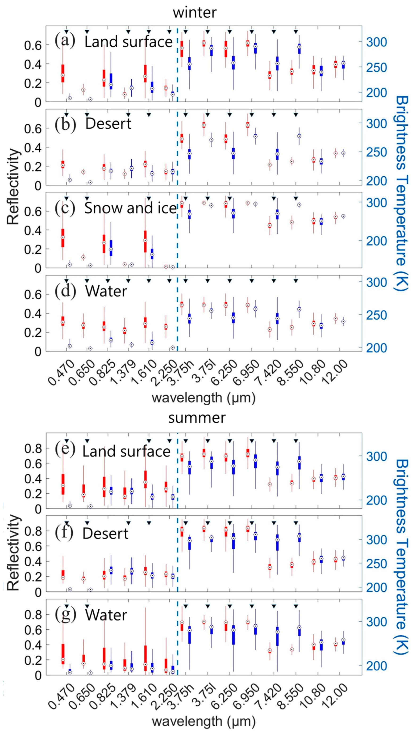
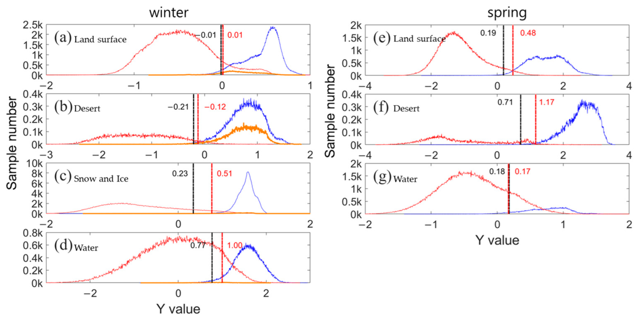
The channels used in the AFDA were selected by the contrasts between cloudy and cloud-free pixels. As shown in Figure 6, channels with obvious differences were selected over four kinds of underlying surfaces. The coefficients of the AFDA formula and the adjusted thresholds of y-values are shown in

Table 2. AFDA function coefficients and thresholds of AGRI in winter and summer.

	Winter				Summer
	Land	Desert	Water	Snow	Land	Desert	Water
0.47 μm	−0.185	0.132	0.885	0.219	−1.127	−0.392	1.569
0.65 μm	−0.078	−0.760	−1.316	0.344	1.182	0.268	−1.573
0.83 μm	―	―	0.296	―	―	―	―
1.37 μm	0.108	0.207	0.165	―	―	0.903	―
1.61 μm	−0.140	−0.276	−0.069	−1.518	−0.634	0.126	―
2.22 μm	0.211	―	−0.270	―	0.343	―	―
3.72 μm (high)	−0.193	−0.632	0.114	0.018	1.016	0.853	−0.102
3.72 μm (low)	−0.041	1.164	−0.292	−0.599	1.309	−1.798	−0.542
6.25 μm	−0.070	−0.541	−0.006	0.046	0.446	0.330	1.541
7.10 μm	0.037	0.587	0.147	―	−0.986	−0.564	−2.196
8.50 μm	−1.032	−1.452	−1.803	−1.663	−0.432	1.717	−1.602
10.8 μm	1.597	1.779	2.245	2.731	2.408	1.629	3.427
12.0 μm	―	―	―	―	―	―	―
13.5 μm	―	―	―	―	―	―	―
y0	0.010	−0.124	0.510	1.000	0.477	1.166	0.170

, and the probability distributions of the y-values are shown in Figure 7. The adjusted thresholds were determined to preserve most of the cloud-free regions, with the y-values greater than y₀ classified as cloud-free, and the others classified as cloudy. As can be seen, some of the cloudy samples had a y-value greater than y₀, an indication that these pixels would be misclassified into the cloud-free group.

3.5. Spectral Spatial Variability Algorithm Construction

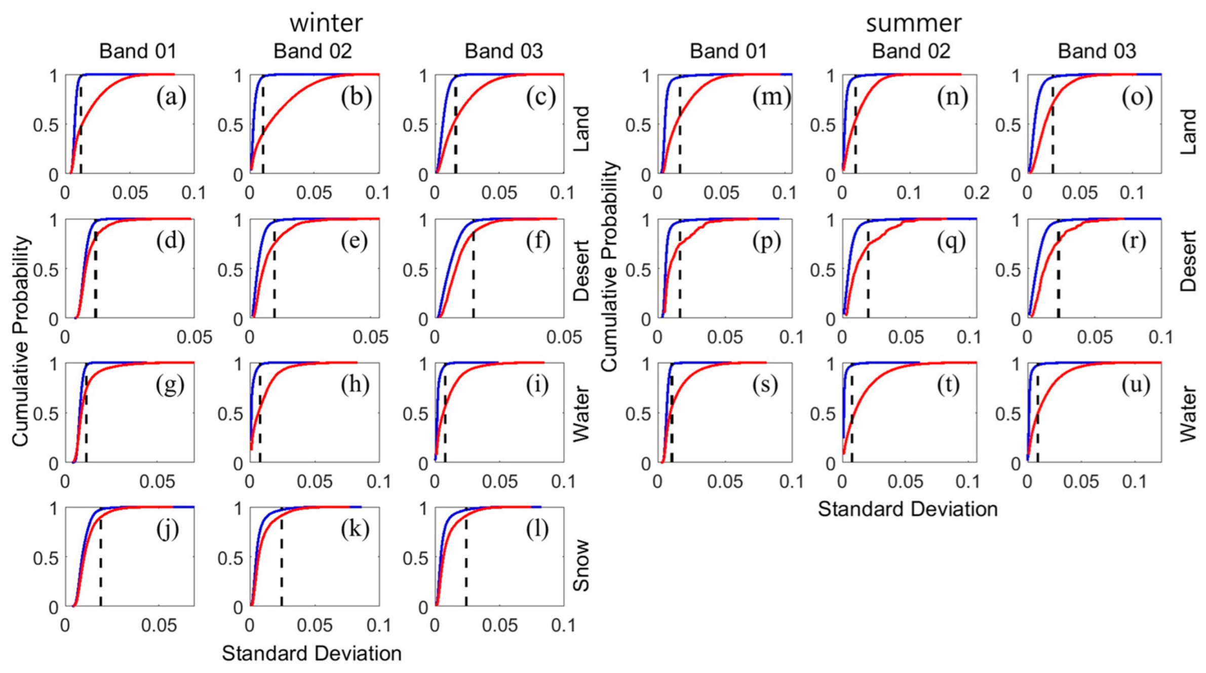
Compared with an overcast FOV, the apparent reflection of ones with broken clouds is more susceptible to radiation reflected by the surface, leading to a higher possibility of being misclassified by AFDA. The 3 × 3 STD was calculated regarding the three visible bands (0.47 μm, 0.65 μm, and 0.83 μm). Cumulative distribution functions (CDFs) were built regarding three channels of clear and misclassified cloudy pixels. As shown in Figure 8, most of the clear pixels had a small STD, and the ones of cloudy pixels were bigger. The thresholds were selected at the 99th percentiles of clear pixels, dividing the pixels with the STD of any of the three channels greater than the corresponding thresholds as cloudy.

4. Performance Assessment

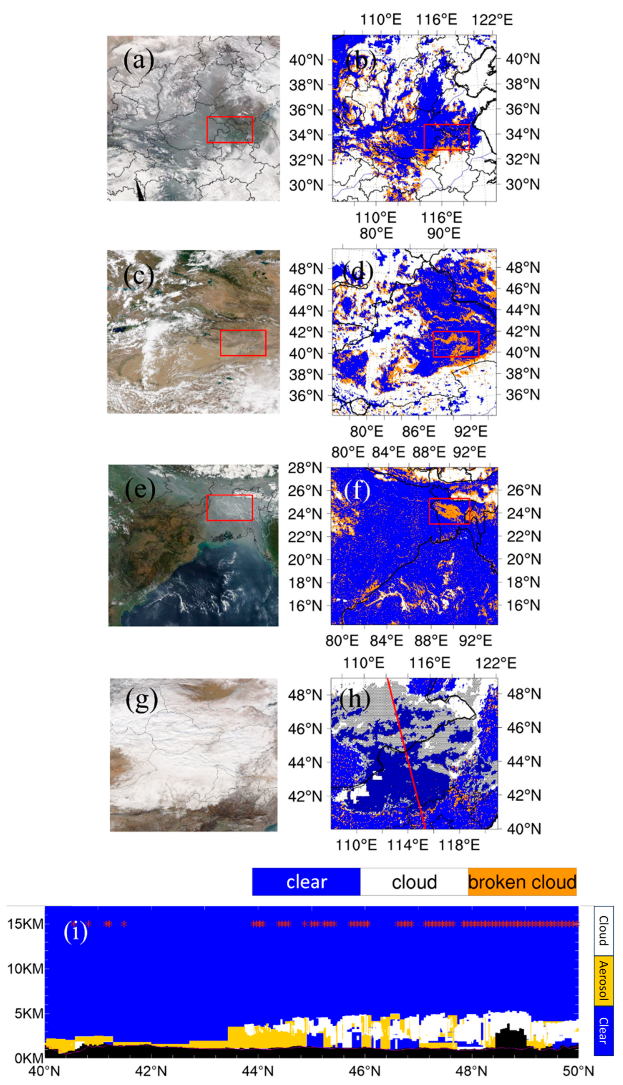
Figure 9 shows the detection results for four different kinds of underlying surfaces. As can be seen, this algorithm showed a robust performance in the hazy regions (Figure 9a,b,e,f), Taklamakan Desert (Figure 9c,d), and water (Figure 9e,f). It is worth noticing that this algorithm could detect the thin or broken clouds over all kinds of underlying surfaces, including the broken clouds at the edge of cloud clusters over the haze regions in East China (Figure 9a,b), the fair weather cumulus over the western part of the Taklamakan Desert in the red rectangle (Figure 9c,d), and the broken clouds over the dense aerosol in North India (Figure 9e,f). Most of the broken clouds were detected by the SSV method. A combination of the two methods, which were AFDA and SSV, increased the sensitivity of the algorithm without increasing the possibility of mistaking the ambiguous targets as clouds. In the detection, AFDA in this algorithm identified most of the cloud clusters, and STD played an important role in the broken clouds’ distinguishment.

Assessment over the snow regions demonstrated that this algorithm recognized most of the clouds over the snow. In Figure 9i, a majority of clouds north of 43° N were detected, except for some thin clouds. The snow’s influence on visible bands, the similar temperature between the snow and cloud top, and the large satellite zenith angle at the high latitude increased the difficulty of cloud detection.

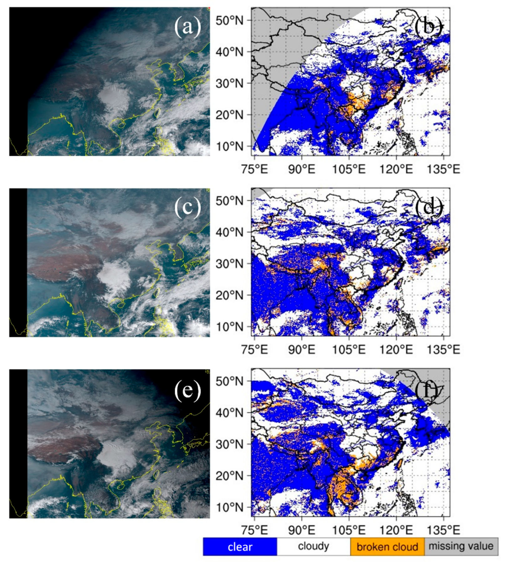
As the Aqua satellite overpassed at about 13:30 local time, all the samples in the algorithm building were observed in the early afternoon. The solar zenith angle is much bigger before mid-morning and after mid-afternoon, which would affect the apparent radiation. Figure 10 shows the detection effects at 1:30, 3:30, and 7:30 UTC, respectively. The results demonstrate that even though the algorithm was built using the samples in the afternoon, it had an excellent performance throughout the daytime.

5. Conclusions

An algorithm based on adjusted Fisher discriminant analysis (AFDA) and spectral spatial variability (SSV) was presented in this paper to realize fast and robust daytime cloud detection of the AGRI/FY-4A detector. Observation of AHI/Himawari-8, rectified cloud mask data of MODIS using the method of Zhang et al. [7], and the vertical feature product (VFM) of CALIPSO were utilized to evaluate the accuracy of AGRI cloud mask, which demonstrated that haze and snow have significant influences on AGRI cloud detection. This study modified the algorithm of Zhang et al. [7] and extended its applicability to China and its surrounding areas, using MODIS observation rectified by the new algorithm as the reference cloud mask data. The cloud detection was achieved by two primary steps. The first step identified cloud clusters by the threshold test on the weighted sum of the normalized spectral data using FDA-derived weight coefficients. The second step captured the broken clouds using the SSV method, which performs a threshold test on the standard deviation of spectral values within a 3 × 3-pixel window. The performance of the algorithm was assessed across four typical regions (East China (EC); the Taklamakan Desert (TD); North India (NI); and North-East China (NEC)), the results of which showed that the algorithm has strong robustness against the interferences of haze and dust pollution, with an accurate distinction between dense aerosols and clouds in EC, the TD, and NI. Compared with the official data, which significantly overestimate the cloud cover in snowy regions, this algorithm showed a much better performance in NEC. Notably, the combination of the SSV method makes this algorithm highly sensitive to broken clouds, including those on the edges of cloud clusters and cellular clouds. Evaluation at three different moments in one day (1:30, 3:30, and 7:30 UTC) showed that this algorithm is applicable in the morning, noon, and afternoon. This algorithm is computationally efficient and suitable for daytime cloud detection in passive satellite remote sensing, realizing accurate detection over most underlying surfaces and primary interferences. Compared with the algorithm of Zhang et al. [7], this one is designed for geostationary satellite detectors, which operate at a much greater distance, and achieves accurate detection of thin and broken clouds.

References

1. Mao, F.; Duan, M.; Min, Q.; Gong, W.; Pan, Z.; Liu, G. Investigating the impact of haze on MODIS cloud detection. J. Geophys. Res. Atmos. 2015, 120, 12–237. [Google Scholar] [CrossRef]
2. Tan, S.C.; Zhang, X.; Wang, H.; Chen, B.; Shi, G.Y.; Shi, C. Comparisons of cloud detection among four satellite sensors on severe haze days in eastern China. Atmos. Ocean. Sci. Lett. 2018, 11, 86–93. [Google Scholar] [CrossRef]
3. Frey, R.A.; Ackerman, S.A.; Liu, Y.; Strabala, K.I.; Zhang, H.; Key, J.R.; Wang, X. Cloud detection with MODIS. Part I: Improvements in the MODIS cloud mask for collection 5. J. Atmos. Ocean. Technol. 2008, 25, 1057–1072. [Google Scholar] [CrossRef]
4. Ackerman, S.A.; Holz, R.E.; Frey, R.; Eloranta, E.W.; Maddux, B.C.; McGill, M. Cloud detection with MODIS. Part II: Validation. J. Atmos. Ocean. Technol. 2008, 25, 1073–1086. [Google Scholar] [CrossRef]
5. Ghosh, R.R.; Ali, M.S.; Hena, A.; Rahman, H. A simple cloud detection algorithm using NOAA-AVHRR satellite data. Int. J. Sci. Eng. Res. 2012, 3, 6. [Google Scholar]
6. Meerkötter, R.; König, C.; Bissolli, P.; Gesell, G.; Mannstein, H. A 14-year European Cloud Climatology from NOAA/AVHRR data in comparison to surface observations. Geophys. Res. Lett. 2004, 31, 15. [Google Scholar] [CrossRef]
7. Zhang, X.; Tan, S.C.; Shi, G.Y.; Wang, H. Improvement of MODIS cloud mask over severe polluted eastern China. Sci. Total Environ. 2019, 654, 345–355. [Google Scholar] [CrossRef] [PubMed]
8. Zhang, X.; Wang, H.; Che, H.Z.; Tan, S.C.; Shi, G.Y.; Yao, X.P. The impact of aerosol on MODIS cloud detection and property retrieval in seriously polluted East China. Sci. Total Environ. 2020, 711, 134634. [Google Scholar] [CrossRef]
9. Li, Z.; Shen, H.; Wei, Y.; Cheng, Q.; Yuan, Q. Cloud detection by fusing multi-scale convolutional features. ISPRS Ann. 2018, 4, 149–152. [Google Scholar] [CrossRef]
10. He, Q.; Sun, X.; Yan, Z.; Fu, K. DABNet: Deformable contextual and boundary-weighted network for cloud detection in remote sensing images. IEEE Trans. Geosci. Remote Sens. 2021, 60, 1–16. [Google Scholar] [CrossRef]
11. Ghasemian, N.; Akhoondzadeh, M. Introducing two Random Forest based methods for cloud detection in remote sensing images. Adv. Space Res. 2018, 62, 288–303. [Google Scholar] [CrossRef]
12. Fu, H.; Shen, Y.; Liu, J.; He, G.; Chen, J.; Liu, P.; Qian, J.; Li, J. Cloud detection for FY meteorology satellite based on ensemble thresholds and random forests approach. Remote Sens. 2018, 11, 44. [Google Scholar] [CrossRef]
13. Xu, L.; Fang, S.; Niu, R.; Li, J. Cloud detection based on decision tree over tibetan plateau with modis data. ISPRS Arch. 2012, 39, 535–538. [Google Scholar] [CrossRef]
14. Zhang, Q.; Yu, Y.; Zhang, W.; Luo, T.; Wang, X. Cloud detection from fy-4a’s geostationary interferometric infrared sounder using machine learning approaches. Remote Sens. 2019, 11, 3035. [Google Scholar] [CrossRef]
15. Tan, K.; Zhang, Y.; Tong, X. Cloud extraction from Chinese high resolution satellite imagery by probabilistic latent semantic analysis and object-based machine learning. Remote Sens. 2016, 8, 963. [Google Scholar] [CrossRef]
16. Ishida, H.; Oishi, Y.; Morita, K.; Moriwaki, K.; Nakajima, T.Y. Development of a support vector machine based cloud detection method for modis with the adjustability to various conditions. Remote Sens. Environ. 2017, 205, 390–407. [Google Scholar] [CrossRef]
17. Shao, Z.; Deng, J.; Wang, L.; Fan, Y.; Sumari, N.S.; Cheng, Q. Fuzzy autoencode based cloud detection for remote sensing imagery. Remote Sens. 2017, 9, 311. [Google Scholar] [CrossRef]
18. Zhang, Y.; Guindon, B.; Cihlar, J. An image transform to characterize and compensate for spatial variations in thin cloud contamination of Landsat images. Remote Sens. Environ. 2002, 82, 173–187. [Google Scholar] [CrossRef]
19. Chen, S.; Chen, X.; Chen, J.; Jia, P.; Cao, X.; Liu, C. An iterative haze optimized transformation for automatic cloud/haze detection of Landsat imagery. IEEE Trans. Geosci. Remote Sens. 2015, 54, 2682–2694. [Google Scholar] [CrossRef]
20. Xiong, Q.; Wang, Y.; Liu, D.; Ye, S.; Du, Z.; Liu, W.; Huang, J.; Su, W.; Zhu, D.; Yao, X.; et al. A cloud detection approach based on hybrid multispectral features with dynamic thresholds for GF-1 remote sensing images. Remote Sens. 2020, 12, 450. [Google Scholar] [CrossRef]
21. Huang, C.; Thomas, N.; Goward, S.N.; Masek, J.G.; Zhu, Z.; Townshend, J.R.; Vogelmann, J.E. Automated masking of cloud and cloud shadow for forest change analysis using Landsat images. Int. J. Remote Sens. 2010, 31, 5449–5464. [Google Scholar] [CrossRef]
22. Irish, R.R.; Barker, J.L.; Goward, S.N.; Arvidson, T. Characterization of the Landsat-7 ETM+ automated cloud-cover assessment (ACCA) algorithm. Photogramm. Eng. Remote Sens. 2006, 72, 1179–1188. [Google Scholar] [CrossRef]
23. Scaramuzza, P.L.; Bouchard, M.A.; Dwyer, J.L. Development of the Landsat data continuity mission cloud-cover assessment algorithms. IEEE Trans. Geosci. Remote Sens. 2011, 50, 1140–1154. [Google Scholar] [CrossRef]
24. Zortea, M.; Salberg, A.B.; Trier, Ø.D. Object-based cloud and cloud shadow detection in landsat images for tropical forest monitoring. In Proceedings of the 4th GEOBIA, Rio de Janeiro, Brazil, 7–9 May 2012; pp. 326–331. [Google Scholar]
25. Zhu, X.; Helmer, E.H. An automatic method for screening clouds and cloud shadows in optical satellite image time series in cloudy regions. Remote Sens. Environ. 2018, 214, 135–153. [Google Scholar] [CrossRef]
26. Surya, S.R.; Simon, P. Automatic Cloud Detection Using Spectral Rationing and Fuzzy Clustering. In Proceedings of the 2013 2nd International Conference on Advanced Computing, Networking and Security, Mangalore, India, 15–17 December 2013; pp. 90–95. [Google Scholar]
27. Bo, P.; Su, F.Z.; Meng, Y.S. A cloud and cloud shadow detection method based on fuzzy c-means algorithm. IEEE J. Sel. Top. Appl. Earth Observ. Remote Sens. 2020, 13, 1714–1727. [Google Scholar] [CrossRef]
28. Ma, N.; Sun, L.; Zhou, C.; He, Y. Cloud detection algorithm for multi-satellite remote sensing imagery based on a spectral library and 1D convolutional neural network. Remote Sens. 2021, 13, 3319. [Google Scholar] [CrossRef]
29. Yang, J.; Zhang, Z.; Wei, C.; Lu, F.; Guo, Q. Introducing the new generation of Chinese geostationary weather satellites, Fengyun-4. Bull. Am. Meteorol. Soc. 2017, 98, 1637–1658. [Google Scholar] [CrossRef]
30. Lu, F.; Zhang, X.; Chen, B.; Liu, H.; Wu, R.; Han, Q.; Feng, X.; Li, J.; Zhan, Z. FY-4 geostationary meteorological satellite imaging characteristic and its application prospects. J. Mar. Meteorol. 2017, 37, 1–12. [Google Scholar]
31. Zhang, P.; Zhu, L.; Tang, S.; Gao, L.; Chen, L.; Zheng, W.; Han, X.; Chen, J.; Shao, J. General comparison of FY-4A/AGRI with other GEO/LEO instruments and its potential and challenges in non-meteorological applications. Front. Earth Sci. 2019, 6, 224. [Google Scholar] [CrossRef]
32. Martins, J.V.; Tanré, D.; Remer, L.; Kaufman, Y.; Mattoo, S.; Levy, R. MODIS cloud screening for remote sensing of aerosols over oceans using spatial variability. Geophys. Res. Lett. 2002, 29, MOD4-1. [Google Scholar] [CrossRef]
33. Chen, B.Y.; Qiong, W.U.; Feng, X.; Guo, Q.; Wei, C.Y. On-orbit test to FY-4A AGRI and generating RBG imagine. J. Infrared Millim. Waves 2018, 37, 411–415. [Google Scholar]
34. Strabala, K.I. MODIS Cloud Mask User’s Guide; University of Wisconsin—Madison: Madison, WI, USA, 2005. [Google Scholar]
35. Winker, D.M.; Hostetler, C.; Vaughan, M.; Omar, A. CALIOP Algorithm Theoretical Basis Document, Part 1: CALIOP Instrument, and Algorithms Overview, Release. J. Atmos. Ocean. Technol. 2006, 26, 2310–2323. [Google Scholar] [CrossRef]
36. Winker, D.M.; Vaughan, M.A.; Omar, A.; Hu, Y.; Powell, K.A.; Liu, Z.; Hunt, W.H.; Young, S.A. Overview of the CALIPSO Mission and CALIOP Data Processing Algorithms. J. Atmos. Ocean. Technol. 2009, 26, 2310–2323. [Google Scholar] [CrossRef]
Figure 1. Flowchart of cloud detection algorithm for AGRI.
Atmosphere 16 01105 g001
Figure 2. (a,f) MODIS/Aqua true-color images, (b,g) AHI/Himawari-8 cloud fractions, (c,h) MODIS cloud masks, (d,i) AGRI/FY-4A cloud masks, and (e,j) CALIPSO vertical feature mask (VFM) profiles along track in (ae) 30 January 2020, and (fj) 27 December 2020. The yellow region in (c,h) is the misjudged “clouds” which was identified with the algorithm of Zhang et al. [7]. The red lines in (c,d,h,i) are the orbit track of CALIPSO. The red dots and green asterisks in (e,j) are the AGRI cloud mask and rectified MODIS cloud mask, respectively, the y-values of which are the retrieved cloud top height, and the red dots under the longitude axis are the AGRI-detected clouds without an effective cloud top height value. The purple lines in (e,j) are the surface elevation along the CALIPSO track.
Atmosphere 16 01105 g002
Figure 3. (ag) True-color images, (hn) cloud masks of AHI, and (ou) cloud masks of AGRI at 01:30 (the first column) to 07:30 (the last column) UTC on 27 December 2020.
Atmosphere 16 01105 g003
Figure 4. (a,d,g) MODIS true-color images, (b,e,h) MODIS cloud masks before (white and orange area) and after (white area) rectification, and (c,f,i) AHI cloud masks on (ac) January 28th, (df) January 2nd, and 25 December 2019. J is the CALIPSO VFM profile along the track in (gi). Orange asterisks in (j) show the MODIS-detected clouds, the y-values of which demonstrate the retrieved cloud top height. The red lines in (g,h,i) are the orbit track of CALIPSO. The red dots and green asterisks in (j) are the AGRI cloud mask and rectified MODIS cloud mask, respectively, the y-values of which are the retrieved cloud top height, and the red dots under the longitude axis are the AGRI-detected clouds without an effective cloud top height value. The purple lines in (e,j) are the surface elevation along the CALIPSO track.
Atmosphere 16 01105 g004
Figure 5. (ac) MODIS true-color images and (df) cloud masks before and after the rectification using the adjusted rectification algorithm on (a,d) January 28th, (b,e) January 2nd, and (c,f) 25 December 2019.
Atmosphere 16 01105 g005
Figure 6. Box charts of reflectivity and BT of FY-4A’s 14 bands over (a,e) land surface, (b,f) desert, (c) snow and ice, and (d,g) water collected in (ad) winter (December and January) and (eg) summer (July and August). Red boxes correspond to the cloudy pixels, and blue boxes correspond to the cloud-free pixels. The left y-axis corresponds to the reflectivity within the solar spectrum (0.47 to 2.25 μm), and the right y-axis corresponds to the BT within the emission spectrum of the land–atmosphere system (3.75 to 12 μm). Black inverted triangles above the boxes demonstrate that the channels were selected for AFDA.
Atmosphere 16 01105 g006
Figure 7. Probability distributions of y-values for cloudy pixels (red line), cloud-free pixels (blue line), and MODIS-misclassified “cloudy” pixels (yellow line). The black dashed lines demonstrate the original thresholds y0 determined by the traditional Fisher discrimination analysis, and the red dashed lines demonstrate the adjusted thresholds y.
Atmosphere 16 01105 g007
Figure 8. STD of 3 × 3 of reflection of bands at 0.47 μm, 0.65 μm, and 0.83 μm over 4 kinds of surfaces in winter and summer. Blue and red lines correspond to the cumulative probability of the STD in clear and cloudy conditions misclassified by AFDA, respectively. Dotted lines are threshold of the STD.
Atmosphere 16 01105 g008
Figure 9. (a,c,e,g) MODIS true-color images, (b,d,f,h) cloud detection results on (a,b) January 28th, (c,d) July 6th, (e,f) January 27th, and (g,h) 27 December 2020, and (i) the VFM cloud and aerosol mask profile on 27 December 2020. The shadow area in (h) shows the snowy region in the FY-4 cloud mask product, and the orange asterisks in (i) show the clouds detected by the AGRI. The red line in (h) shows the orbit of CALIPSO.
Atmosphere 16 01105 g009
Figure 10. (a,c,e) AHI true-color images and (b,d,f) AGRI cloud detection results at UTC 1:30, 3:30, and 7:30 on December 28th.
Atmosphere 16 01105 g010