Simulations of Drainage Flows with Topographic Shading and Surface Physics Inform Analytical Models

Abstract

We perform large-eddy simulations (LESs) with realistic radiation, including topographic shading, and an advanced land surface model to investigate drainage flow dynamics in an idealized compound-slope mountain geometry. This allows an analysis not only of fully developed profiles in steady state—the subject of existing analytical solutions—but also of transient two- and three-dimensional dynamics. The evening onset of downslope flow is related to the duration of shadow front propagation along the eastern slopes, for which an analytic form is derived. We demonstrate that the flow response to this radiation pattern is mediated by the thermal inertia of the land through sensitivity to soil moisture. Onset timing differences on opposite sides of the peak are explained by convective structures that persist after sunset over the western slopes when topographic shading is considered. Although these preceding convective systems, as well as the presence of neighboring terrain, inhibit the initial development of drainage flows, the LES develops an approximately steady-state, fully developed flow over the finite slopes and finite nocturnal period. This allows a comparison to analytical models restricted to such cases. New analytical solutions based on surface heat flux boundary conditions, which can be estimated by the coupled land surface model, suggest the need for improved representation of the eddy diffusivity for analytical models of drainage flows.

1. Introduction

Drainage flows—downslope flows driven by the buoyancy that results from surface cooling on sloped terrain—are important processes in the atmospheric boundary layer. Drainage flows converge in topographic depressions and strengthen the stable stratification that traps pollutants in basins such as the Salt Lake Valley in Utah [1]. Fire weather is also directly affected by slope flows, where including the effect of drainage flows on fuel moisture is considered paramount for the safety of firefighters [2]. Despite these critical needs, the inaccurate representation of drainage flow dynamics contributes significantly to near-surface temperature biases in numerical weather prediction (NWP) models [3,4]. Even at fine spatial scales, numerical stability limits related to sloped terrain [4,5,6] can make it prohibitively expensive to explicitly resolve drainage flows [7].

Given the limitations of brute-force computation, we analyze drainage flows across a hierarchy of model complexities instead. We begin with the simplest model of drainage flows, an analytical solution first presented by Prandtl [8]. The work of Grisogono and Oerlemans [9] continues this line of analytical modeling but adds complexity by presenting a solution that allows variable eddy diffusivity. While these analytical solutions help to build our intuition regarding the dynamics of drainage flows at steady state, they do not address the temporal and spatial development of drainage flows. In the classic Prandtl solution, a negative temperature perturbation is prescribed as a Dirichlet boundary condition. In reality, the temperature of the surface is determined by an energy budget that is externally forced by radiation. As such, we expect the time development of drainage flows to depend on the pattern of solar radiation, which can be significantly altered by the presence of topography. A relevant timescale is then the duration of shadow front propagation along a slope. A separate timescale is set by the thermal inertia of the land. The persistence of daytime convection is also seen to affect the timing of the evening onset of drainage flows. To investigate these effects, which are absent in one-dimensional analytical solutions, we use an advanced numerical weather prediction (NWP) model, which uses radiation physics including topographic shading to force a land surface model, at the most complex end of our model hierarchy.

Studies of drainage flow onset have been performed in NWP models for real weather cases, e.g., using the Weather Research and Forecasting (WRF) model with an ultra-fine resolution at Granite Mountain, Utah [10], but fundamental relationships are difficult to discern from such simulations. In real terrain simulations, even simple parameters required for comparison to analytical solutions, e.g., the slope angle, can be ambiguous. To avoid this ambiguity, semi-idealized high-resolution simulations are performed here in WRF with a simple terrain geometry with a compound slope. This semi-idealized model allows transient solutions to be obtained with large-eddy simulation (LES), topographic shading, and a coupled land surface model.

Additionally, our LES results are compared to existing and novel analytical solutions in regions of sufficiently developed flow, where an approximately steady-state model solution is obtained. Differences between the numerical and previous analytical models are found to be associated with the surface boundary condition. New analytical solutions are then derived, which incorporate the surface heat flux approximated by WRF. Variants that either retain the simplicity of the classic Prandtl solution or allow a more sophisticated representation of turbulence are presented.

2. Background

2.1. The Prandtl Solution

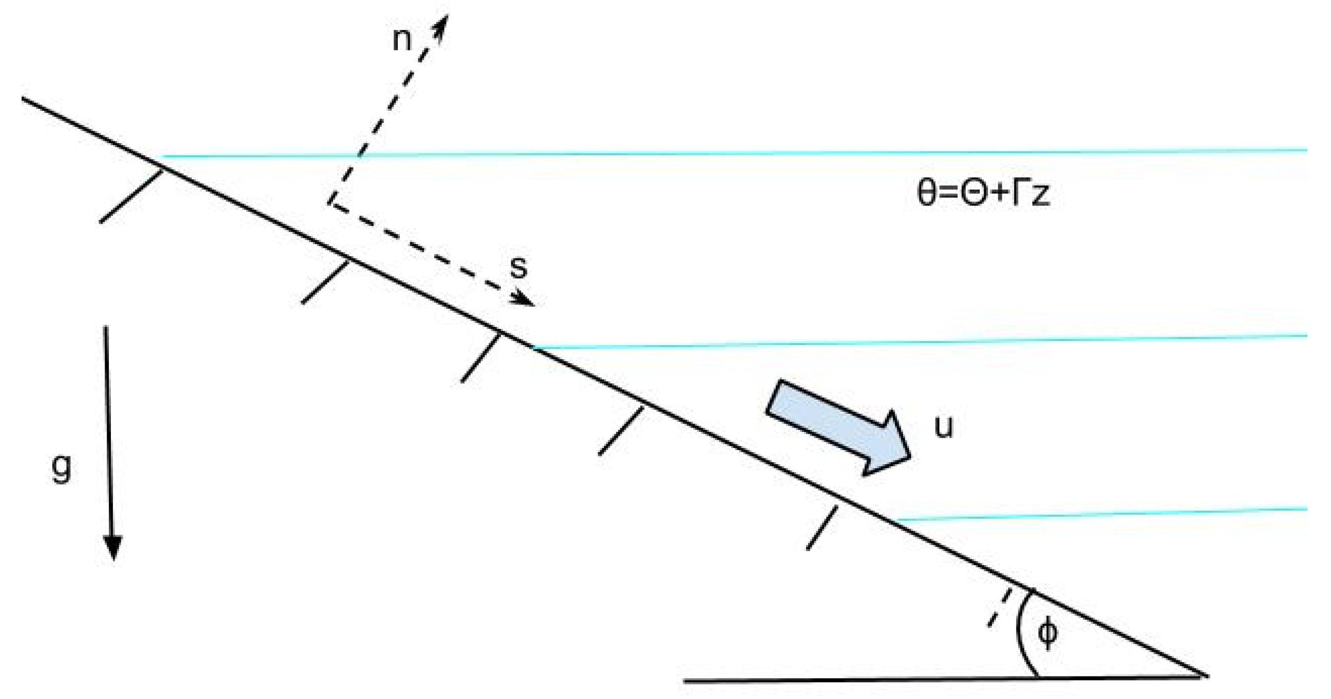
Prandtl [8] presented and solved the equations governing a drainage flow in the simplest possible geometry, shown in Figure 1. For convenience, axes are rotated normal to the slope, n, and pointing downslope, s, parallel to the land surface, which is inclined at an angle, $\varphi$, such that the elevation is $z=ncos\varphi -ssin\varphi$. The positive lapse rate, $\mathrm{\Gamma }$, of a stable background profile maintained by a regional energy balance is assumed constant. Then, the potential temperature field is

$$\begin{array}{cc}\hfill \theta & ={\theta }_0+\mathrm{\Gamma }(ncos\varphi -ssin\varphi )+{\theta }^{\prime }\left(n\right),\hfill \end{array}$$

(1)

assuming a fully developed flow in s and an infinite incline to neglect variations into and out of the page as well. At steady sate, the conservation of internal energy may be expressed as a transport equation for temperature in this setting:

$$\begin{array}{cc}\hfill u{\displaystyle \frac{\partial \theta }{\partial s}}=& -{\displaystyle \frac{\partial J}{\partial n}}.\hfill \end{array}$$

(2)

The analytical models neglect radiation and other less significant physical terms in the near-slope region, such that the flux, J, is entirely due to turbulence. Prandtl models this as $J=-K_H{\displaystyle \frac{\partial \theta }{\partial n}}$ with a constant $K_H$, the eddy diffusivity. Note that all non-linear variations of $\theta$ given by Equation (1) are contained in the ${\theta }^{\prime }\left(n\right)$ term such that this turbulent diffusion term reflects temperature perturbations rather than the temperature itself. The LHS can be evaluated directly from Equation (1), so that the final form of the internal energy equation in the Prandtl model is

$$\begin{array}{cc}\hfill -u\mathrm{\Gamma }sin\varphi & =K_H{\displaystyle \frac{{\partial }^2{\theta }^{\prime }}{\partial n^2}}.\hfill \end{array}$$

(3)

Turning our attention to the momentum equation, we retain the assumption of a steady flow on an infinite plane, fully developed in the along-slope direction. Further assuming no external pressure gradient and neglecting the hydrostatic contribution in s, which is suitable for angles less than 10 degrees [11], the momentum equations are reduced to a balance between the turbulent diffusion of momentum and buoyancy forcing. The turbulent diffusion of momentum is modeled by Prandtl with a constant eddy diffusivity model similar to that used above in the internal energy equation. We take only the s-direction component of the acceleration due to buoyancy familiar from Archimedes’ principle, $f_{b,z}=g{\displaystyle \frac{{\theta }^{\prime }}{{\theta }_{\mathrm{env}}}}$, by multiplying by −$sin\varphi$. We make the additional assumption that the variability associated with ${\theta }^{\prime }$ is greater than that of the environmental lapse rate. That is, ${\theta }_{\mathrm{env}}\approx {\theta }_0$ such that buoyant acceleration is a function of only the temperature perturbation in the final form of the force balance,

$$\begin{array}{c}\hfill 0=K_M{\displaystyle \frac{{\partial }^{2}u}{\partial n^2}}-{\displaystyle \frac{gsin\varphi }{{\theta }_0}}{\theta }^{\prime }.\end{array}$$

(4)

In the classic Prandtl solution, Dirichlet boundary conditions are enforced. The temperature of air at the surface is expected to be in thermal equilibrium with the land surface. Then, for the drainage flow, a negative temperature perturbation is assigned at the bottom boundary. Surface drag is represented by enforcing a no-slip boundary condition at the surface. In the far field, both the velocity and temperature perturbation go to zero. Summarily,

$$\begin{array}{cc}\hfill u(n=0)& =0\hfill \end{array}$$

(5)

$$\begin{array}{cc}\hfill {\theta }^{\prime }(n=0)& ={\theta }_{\mathrm{surface}}-{\theta }_0={\theta }_0^{\prime }\hfill \end{array}$$

(6)

$$\begin{array}{cc}\hfill u(n\to \infty )& =0\hfill \end{array}$$

(7)

$$\begin{array}{cc}\hfill {\theta }^{\prime }(n\to \infty )& =0\hfill \end{array}$$

(8)

specify a unique solution to Equations (3) and (4), the governing equations.

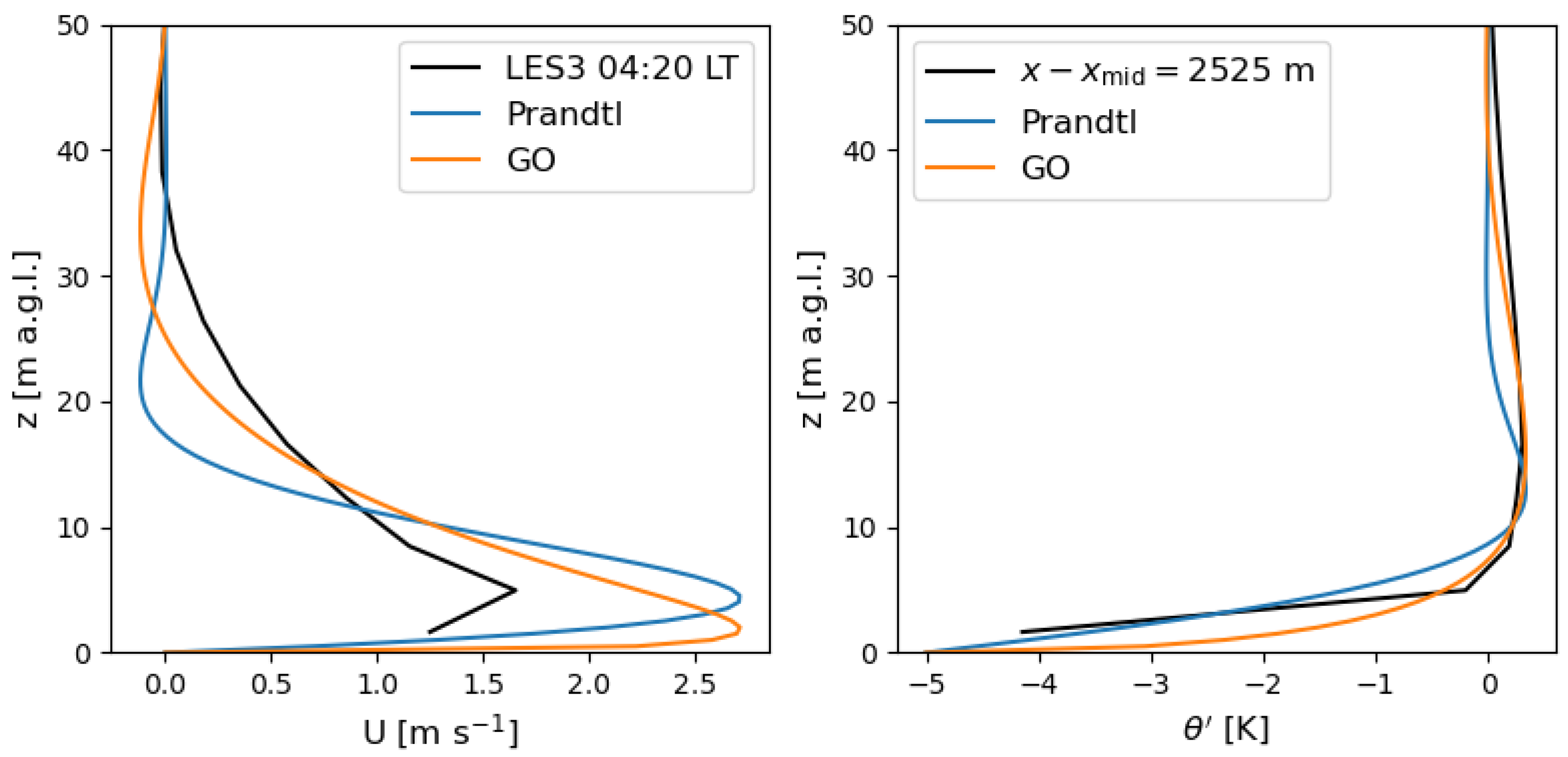
The system of equations may be solved by differentiating either (3) or (4) twice with respect to n to substitute into the other equation and obtain a fourth-order, linear ordinary differential equation. Such equations can be solved with standard techniques and always have the form of a linear combination of complex exponentials. Together with solutions from models described in later sections, Figure 2 shows example profiles of the below Prandtl solution:

$$\begin{array}{cccc}\hfill u=-{\theta }_0^{\prime }& {\left({\displaystyle \frac{g{K}_H}{{\theta }_0\mathrm{\Gamma }{K}_M}}\right)}^{{\displaystyle \frac{1}{2}}}\hfill & \hfill exp\left[-{\left({\displaystyle \frac{g\mathrm{\Gamma }{sin}^2\varphi }{4{\theta }_0{K}_M{K}_H}}\right)}^{{\displaystyle \frac{1}{4}}}n\right]& sin\left[{\left({\displaystyle \frac{g\mathrm{\Gamma }{sin}^2\varphi }{4{\theta }_0{K}_M{K}_H}}\right)}^{{\displaystyle \frac{1}{4}}}n\right]\hfill \end{array}$$

(9)

$$\begin{array}{cccc}\hfill {\theta }^{\prime }=& {\theta }_0^{\prime }\hfill & \hfill exp\left[-{\left({\displaystyle \frac{g\mathrm{\Gamma }{sin}^2\varphi }{4{\theta }_0{K}_M{K}_H}}\right)}^{{\displaystyle \frac{1}{4}}}n\right]& cos\left[{\left({\displaystyle \frac{g\mathrm{\Gamma }{sin}^2\varphi }{4{\theta }_0{K}_M{K}_H}}\right)}^{{\displaystyle \frac{1}{4}}}n\right].\hfill \end{array}$$

(10)

Note that the effect of the cold ground is confined to a relatively shallow layer. The location of the first maximum above the surface, $n_{\max }$, is a characteristic height for this shallow flow defined such that $u\left(n_{\max }\right)=u_{\max }$. From (9), we obtain

$$\begin{array}{cc}\hfill n_{\max }& ={\displaystyle \frac{\pi }{4}}{\left({\displaystyle \frac{g\mathrm{\Gamma }{sin}^2\varphi }{4{\theta }_0{K}_M{K}_H}}\right)}^{-{\displaystyle \frac{1}{4}}}\hfill \end{array}$$

(11)

$$\begin{array}{cc}\hfill u_{\max }& =-{\theta }_0^{\prime }{\left({\displaystyle \frac{g{K}_H}{{\theta }_0\mathrm{\Gamma }{K}_M}}\right)}^{{\displaystyle \frac{1}{2}}}{e}^{-{\displaystyle \frac{\pi }{4}}}{\displaystyle \frac{\sqrt{2}}{2}}.\hfill \end{array}$$

(12)

When these results are compared to field observations, we find that the values of $n_{\max }$ and $u_{\max }$ predicted by Prandtl are often too large [12]. Several simplifying assumptions are possible reasons for this deficiency. One possibility is the assumption of constant eddy diffusivities. From the scale height, $n_{\max }$, we see that lower diffusivities correspond to shallower jets. As the eddy mixing lengths are limited by the distance to the wall, a variable diffusivity should be near its minimum near the surface. An analytical model accounting for this variability will therefore lead to an even shallower drainage flow than predicted by the Prandtl model.

Before presenting the variable diffusivity case, it is convenient to note an abbreviated form of the Prandtl solution

$$\begin{array}{cc}\hfill F& =exp[-(1+i\left)\sigma n\right]\hfill \end{array}$$

(13)

$$\begin{array}{cc}\hfill u& ={\theta }_0^{\prime }\mu Im\left(F\right)\hfill \end{array}$$

(14)

$$\begin{array}{cc}\hfill {\theta }^{\prime }& ={\theta }_0^{\prime }Re\left(F\right)\hfill \end{array}$$

(15)

where

$$\begin{array}{cc}\hfill \sigma & ={\left({\displaystyle \frac{g\mathrm{\Gamma }{sin}^2\varphi }{4{\theta }_0{K}_M{K}_H}}\right)}^{{\displaystyle \frac{1}{4}}}\left[{\mathrm{m}}^{-1}\right]\hfill \end{array}$$

(16)

$$\begin{array}{cc}\hfill \mu & ={\left({\displaystyle \frac{g{K}_H}{{\theta }_0\mathrm{\Gamma }{K}_M}}\right)}^{{\displaystyle \frac{1}{2}}}\left[\mathrm{m}{\mathrm{s}}^{-1}{\mathrm{K}}^{-1}\right].\hfill \end{array}$$

(17)

2.2. The Grisogono and Oerlemans Solution

Grisogono and Oerlemans [9] give another solution—hereafter the GO solution—by considering drainage flows with variable eddy diffusivities and employing the Wentzel–Kramers–Brillouin (WKB) method for approximating solutions to differential equations. The WKB method is limited to cases where diffusivities change only gradually and are prescribed functions of n, the distance from the surface. The diffusivities for the velocity and temperature are required to have the same functional form for a constant Prandtl number. With these restrictions, the governing equations are

$$\begin{array}{cc}\hfill 0& ={\displaystyle \frac{\partial }{\partial n}}\left[K_H\left(n\right){\displaystyle \frac{\partial {\theta }^{\prime }}{\partial n}}\right]+u\mathrm{\Gamma }sin\varphi \hfill \end{array}$$

(18)

$$\begin{array}{cc}\hfill 0& ={\displaystyle \frac{\partial }{\partial n}}\left[K_M\left(n\right){\displaystyle \frac{\partial u}{\partial n}}\right]-{\displaystyle \frac{gsin\varphi }{{\theta }_0}}{\theta }^{\prime }\hfill \end{array}$$

(19)

which resemble the governing equations in the Prandtl model, (3) and (4), but with more sophisticated diffusion terms. Further, the GO solution below resembles the Prandtl solution in complex form (Equations (13)–(17))

$$\begin{array}{cc}\hfill F& =exp\left[-(1+i){\left({\sigma }_0/2\right)}^{1/2}{\int }_0^n{K}_H^{-{\displaystyle \frac{1}{2}}}\left(n^{\prime }\right)d{n}^{\prime }\right]\hfill \end{array}$$

(20)

$$\begin{array}{cc}\hfill u& ={\theta }_0^{\prime }\mu Im\left(F\right)\hfill \end{array}$$

(21)

$$\begin{array}{cc}\hfill {\theta }^{\prime }& ={\theta }_0^{\prime }Re\left(F\right)\hfill \end{array}$$

(22)

where

$$\begin{array}{cc}\hfill {\sigma }_0^2& ={\displaystyle \frac{g\mathrm{\Gamma }{sin}^2\varphi }{{\theta }_0\mathrm{Pr}}}\left[{\mathrm{s}}^{-2}\right]\hfill \end{array}$$

(23)

$$\begin{array}{cc}\hfill \mathrm{Pr}& ={\displaystyle \frac{K_M}{K_H}}[-]\hfill \end{array}$$

(24)

$$\begin{array}{cc}\hfill \mu & ={\left({\displaystyle \frac{g}{{\theta }_0\mathrm{\Gamma }\mathrm{Pr}}}\right)}^{{\displaystyle \frac{1}{2}}}\left[\mathrm{m}{\mathrm{s}}^{-1}{\mathrm{K}}^{-1}\right].\hfill \end{array}$$

(25)

This solution is valid only near the surface, although Grisogono and Oerlemans [9] also give an outer solution, which is omitted here. We adapt the functional form of the original derivation [9],

$$\begin{array}{cc}\hfill K_H^{\mathrm{GO}}& =Cnexp\left[{\displaystyle \frac{-n^2}{2h^2}}\right]\hfill \end{array}$$

(26)

with $C=0.008\mathrm{m}{\mathrm{s}}^{-1}$, h = 20 m, and Pr $=0.75$ for the eddy diffusivities required to calculate and plot the resulting GO solution, shown in Figure 2.

In comparison to the Prandtl solution, gradients near the ground are much sharper in the variable diffusivity case (Figure 2). Although the maximum velocities are roughly equal to those in the Prandtl solution, the jet height is considerably shallower. In this sense, the Grisogono and Oerlemans solutions compare better to certain observations [12] than the Prandtl solutions, but at the cost of adding complexity to the representation of turbulent processes.

Despite the sophistication of the representation of turbulent diffusion in the GO solution, important limitations remain with the eddy diffusion model. An immediate consequence of these mixing length arguments is zero diffusivities at the surface, which poses a challenge in applying a flux boundary condition. At the surface—more precisely, in the viscous sublayer above the surface considered infinitesimally deep—the assumption that mixing is dominated by eddies with length scales limited by the distance to the wall does not apply. In later sections, we relax this constraint on the functional form of the diffusivity used in the down-gradient fluxes. We use non-zero values at the surface and deem the eddy diffusivity “effective” because the mixing cannot be due to eddies with the implied zero length scale at the surface. Rather, the effective diffusivity is defined to fit both the surface heat flux and the temperature perturbation at the surface, thus incorporating the surface processes into the phenomenologically different turbulent processes above.

2.3. Other Models

In the history of drainage flow modeling through computational fluid dynamics (CFD), numerical solutions have been obtained for an increasingly complicated model problem: considering fuller sets of equations [13,14,15,16], adding three-dimensional effects such as slope and valley flow interactions [17], and using more sophisticated turbulence closures [11,12,18]. The computations performed by CFD codes are, however, generally not coupled with any of the sophisticated physics parameterizations, such as the land surface and radiation schemes, that were developed separately in the NWP community. Now, with the aid of high-performance parallel computers, NWP models are able to run at large-eddy-permitting resolutions [19,20]. Commonly, an idealized terrain shape is used [21,22]. Arthur et al. [10] considered drainage flows over real terrain, but with idealized boundary conditions.

We present a semi-idealized model in which advanced radiation and surface flux boundary conditions are employed with an idealized terrain shape. Later, novel analytical solutions are presented and evaluated using the surface heat flux estimated by the model. A variant employing constant eddy diffusivities rectifies discrepancies in the dependence on the slope angle between the Prandtl model and the current and previous LES [11,12,18]. Subsequent model development integrates an effective eddy diffusivity approach into the GO solution. This allows the imposition of more realistic surface heat flux boundary conditions, as well as the use of variable eddy diffusivities.

3. Methods

The WRF-LES simulations are configured to represent a set of idealized model topographies (

Table 1. WRF-LES model topography parameters and initial soil moisture values.

Simulation	${\mathit{\varphi }}_1{[}^{\circ }]$	${\mathit{L}}_1$ [km]	${\mathit{\varphi }}_2{[}^{\circ }]$	${\mathit{L}}_2$ [km]	Soil Mois. $m^3$ $m^{-3}$
LES2	2	4.502	5	1	0.0868
LES3	3	3	5	1	0.0868
LES4	4	2.248	5	1	0.0868
DRY3	3	3	5	1	0.0434

). The shape of the ideal terrain is defined by each side having a long, shallow slope (the foothills) below a shorter, steeper slope at the mountain peak. During the evening transition, the shadow of the steeper slope is cast onto the lower slope. The length of the lower slopes is varied to maintain a consistent peak height but sufficient distance for a flow to fully develop. The lengths and slopes are as labeled in Figure 3, and the terrain height is defined as

$$h\left(x;{\varphi }_1,L_1,{\varphi }_2,L_2\right)=\left\{\begin{array}{cc}0\hfill & for|x-x_{\mathrm{mid}}|\ge L_1+L_2\hfill \\ tan{\varphi }_1\left(L_1+L_2-|x-x_{\mathrm{mid}}|\right)\hfill & for{L}_2<|x-x_{\mathrm{mid}}|<L_1+L_2\hfill \\ tan{\varphi }_1{L}_1+tan{\varphi }_2\left(L_2-|x-x_{\mathrm{mid}}|\right)\hfill & for|x-x_{\mathrm{mid}}|\le L_2\hfill \end{array}\right.$$

(27)

where $x_{\mathrm{mid}}=9975$ m is the midpoint of the domain and $h\left(x_{\mathrm{mid}}\right)=245$ m in all simulations. With this 2D terrain, variations in velocity and potential temperature due to resolved turbulence can be averaged out in the y (south–north) direction, so the profiles can be compared to those from the analytical solutions.

The ridge is aligned south–north, so the shadow of the upper slope may be cast onto the lower slope at sunrise and sunset. The incident shortwave radiation flux is nearly constant in the south–north direction by locating the mountain on a fictitious landmass at $0^{\circ }$ N, $0^{\circ }$ W and by simulating insolation on the vernal equinox, 20 March 2014. On this date, the LES runs are initialized at 12:00 LT (UTC+0) and analyzed from this time until the morning of the following day. Initial conditions are quiescent winds and a stable lapse rate of 3 K ${\mathrm{km}}^{-1}$ starting at 305 K at 25 m until a height of 12 km above sea level. The initial surface skin temperature is set to 310 K and initial humidity is set to 10 g ${\mathrm{kg}}^{-1}$ everywhere. Periodic boundary conditions are used along lateral boundaries.

Subgrid parameterizations employed in the LES include a turbulent kinetic energy (TKE) 1.5-order LES turbulence closure [23,24] coupled with a surface-layer parameterization [25] based on Monin–Obukhov similarity theory (MOST) [26]. The specific implementation of the surface layer scheme has been updated to handle the wide range of stability parameters present in the simulations [27,28]. Additional physical parameterizations include the Rapid Radiative Transfer Model for longwave radiation [29], the Dudhia shortwave radiation model [30], Zängl’s topographic shading routine [31], and the Noah land surface model [32]. These parameterizations are similar to those recently used for the idealized simulation of valley flows with WRF that included thermally driven, near-surface flows [10].

The current LES setup echoes the configuration of the land model in Arthur et al. [10] as well. Specifically, the land cover type in the model is savannah, corresponding to index 10 from the United States Geological Survey (USGS) classification. The parameters used in WRF for this land cover are a constant roughness length, $z_0$ = 15 cm, and a host of vegetation parameters that are used in the energy balance. However, only the roughness lengths directly impact the dynamics, so the current results may not extend to dense canopies. Parameters important to the the surface energy budget are the albedo and emissivity, which are set to 0.2 and 0.92, respectively. The soil type is sandy loam, initialized with volumetric water content of 0.0868 m $m^{-1}$ in simulations LES2, LES3, and LES4. Another simulation, DRY3, is run with soil moisture initialized to 0.0434 m $m^{-1}$, half that of the other simulations. This tests the sensitivity of the flow to a soil property known to exert strong control on the thermal inertia of the land [3].

All simulations are performed with the WRF model version 3.9.1.1, developed by the National Center for Atmospheric Research [33]. The dynamic core of the model provides a numerical solution to the compressible flow equations with a third-order Runge–Kutta time advancement scheme, with split time stepping to handle acoustic modes, as well as fifth-order horizontal advection and third-order vertical advection. Computations are performed on a mesh with constant and uniform horizontal grid spacing, $\mathsf{\Delta }x=\mathsf{\Delta }y=50$ m, spanning 400 points in the x-direction and 150 points in the y-direction. The grid used is an Arakawa C-staggered grid for which the vertical coordinate is a non-uniform, pressure-based, terrain-following coordinate system. Although the heights of the pressure coordinates evolve dynamically in WRF, every simulation uses roughly the same vertical grid spacing. The vertical grid is designed to stretch from $\mathsf{\Delta }{z}_{\min }=3$ m at the first full model level at 10% per level up to $\mathsf{\Delta }{z}_{\max }=530$ m, above which this maximum grid spacing is maintained until the model top at 12 km elevation, over 69 vertical levels. The LES uses $\mathsf{\Delta }t$ = 0.2 s, following the recommended stability limits for terrain-following coordinate systems [4].

4. Results and Discussion

4.1. Diurnal Cycle

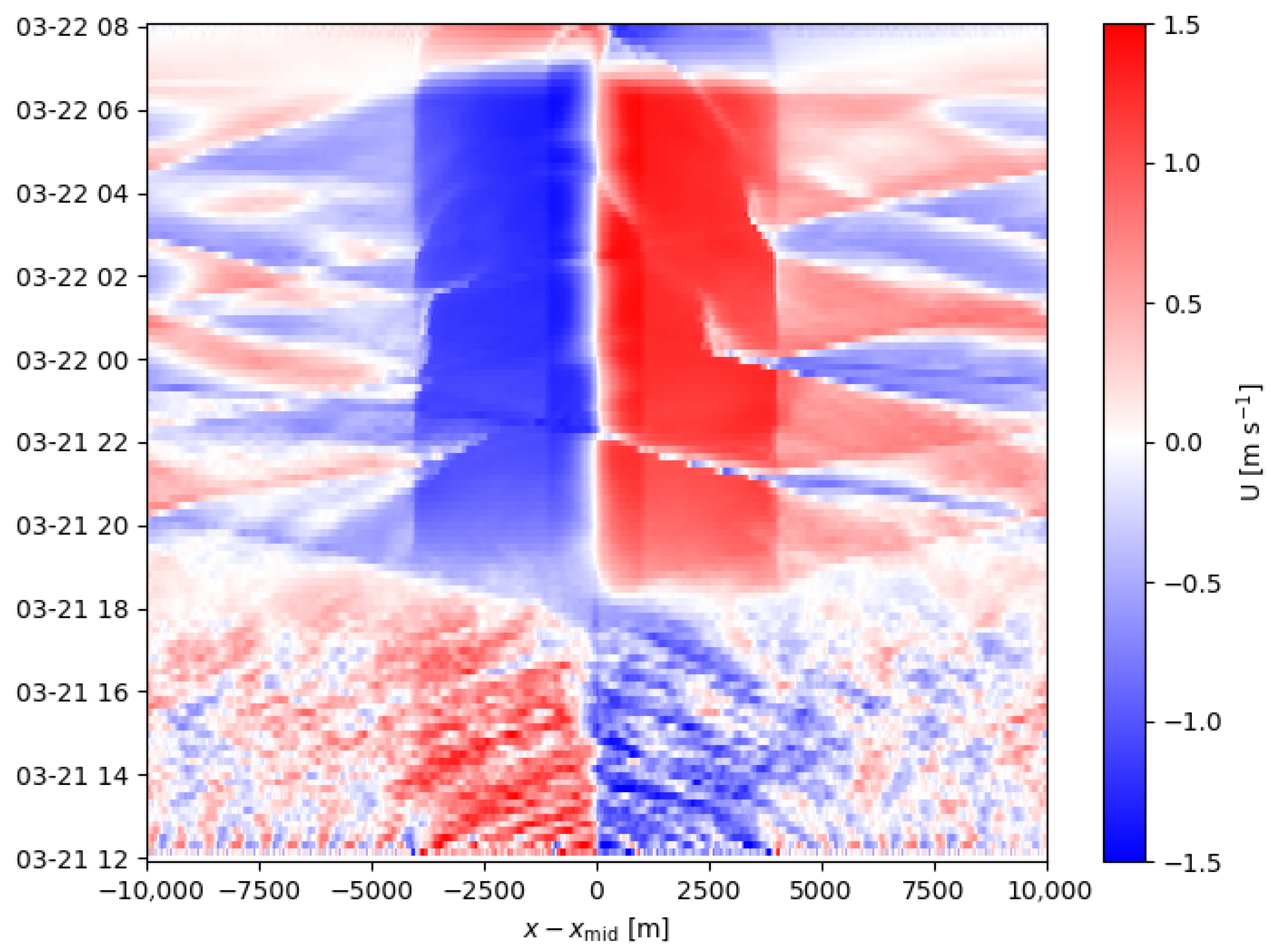
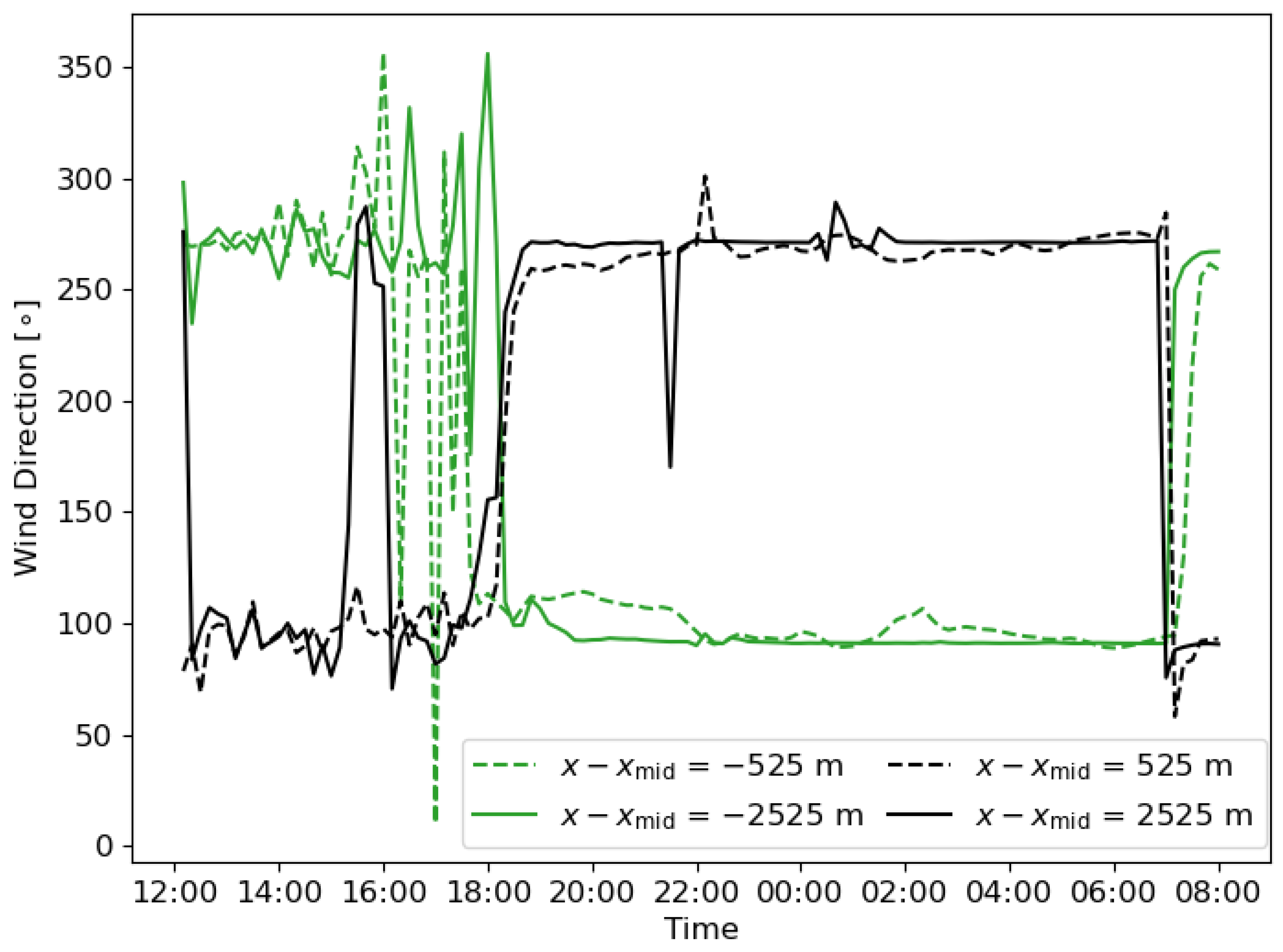
The numerical model recreates the general pattern of the diurnal cycle that is predicted by fundamental theory [34]—thermally driven flows that are upslope during the day and downslope during the night. Figure 4 shows the time evolution of the along-slope (x-direction) velocity from the lowest model half-level, ≈1.5 m a.g.l., averaged in the cross-slope (y) direction. Figure 5 shows the average wind direction from the middle of the four planes that piecewise define the shape of the terrain.

At the beginning of the simulation period (bottom of Figure 4, left of Figure 5), positively buoyant near-surface flows are most often upslope. This manifests as symmetry in the plots, so a sign change (Figure 4) and a rotation by ${180}^{\circ }$ (Figure 5) are notable when comparing opposite sides of the mountain. Later, at around 18:00, these upslope flows begin to transition to downslope flows. This transition eventually occurs on both sides of the peak, but the broken symmetry near the centerline, $x-x_{\mathrm{mid}}$ = 0, due to topographic shading is particularly notable around sunset, 18:00 LT, in the Hovmöller diagram (Figure 4).

In addition to these changes in mean flow, after sunset, there are no sporadic periods of reversed flow, seen as small patches of different colors in Figure 4 from just after initialization at 12:00 LT (bottom) until 18:00 LT, i.e., sunset. These cease because the levels of turbulence are suppressed during the nocturnal period after 18:00 LT until the end of the simulations at 08:00 LT (top). This is apparent in the time series of the wind direction as well, where the variability decreases significantly after the transition to downslope flows begins after 18:00 LT or sunset (Figure 5). There are times of reversed flow (visible as thin red or blue streaks in the Hovmöller diagram), but these are due to the downslope flows from the opposite side of the mountain passing through the periodic boundary, as discussed in more detail below. Near the end of the simulation, around 07:00, the signs of the slope flow are again reversed as an upslope flow is initiated by the return to surface heating after sunrise.

4.2. Sunset

During the evening, a shadow is cast from the mountain peak onto the lower eastern slope. A line can be drawn from the sun to the peak of the mountain and extended to another point on this section of the eastern slope, as drawn in Figure 3, which can be expressed in point-slope form as

$$\left[h\left(x\right)-h\left(x_{\mathrm{mid}}\right)\right]=-cot{\theta }_s\left[x-x_{\mathrm{mid}}\right].$$

(28)

where ${\theta }_s$ is the solar angle.

The intersection of this line and the terrain represents the location of the shadow front as it moves down the slope. Solving the linear system for this point results in a function of the solar angle,

$$cot{\theta }_s=tan{\varphi }_1+{\displaystyle \frac{L_2}{x-x_{\mathrm{mid}}}}\left(tan{\varphi }_2-tan{\varphi }_1\right).$$

(29)

In general, $cos{\theta }_s=sin\Phi sin\delta +cos\Phi cos\delta cos\eta$, where $\Phi$ is the latitude, $\delta$ is the solar declination, and $\eta$ is the hour angle. Considering the current choice to simulate the equator on the equinox, it follows that the solar angle is equivalent to the hour angle,

$${\theta }_s=\eta ={\displaystyle \frac{t-12}{24}}2\pi$$

(30)

where t is in hours. With this substitution and the application of a trigonometric identity for the inverse cotangent in Equation (29), we arrive at

$$t=18-{\displaystyle \frac{12}{\pi }}arctan\left[tan{\varphi }_1+{\displaystyle \frac{L_2}{x-x_{\mathrm{mid}}}}\left(tan{\varphi }_2-tan{\varphi }_1\right)\right].$$

(31)

This form expresses the time of local sunset as the equinox sunset time, 18:00, and an offset due to the terrain. A special case of note, taking $x-x_{\mathrm{mid}}=L_2$, is also equal to the local sunset on the entire upper portion of the eastern slope, because the terrain line and the line traced back to the sun through the mountain peak are coincident for this case. With the slope angle expressed in radians,

$$t_{\mathrm{upper}\mathrm{slope}}=18-{\displaystyle \frac{12}{\pi }}{\varphi }_2.$$

(32)

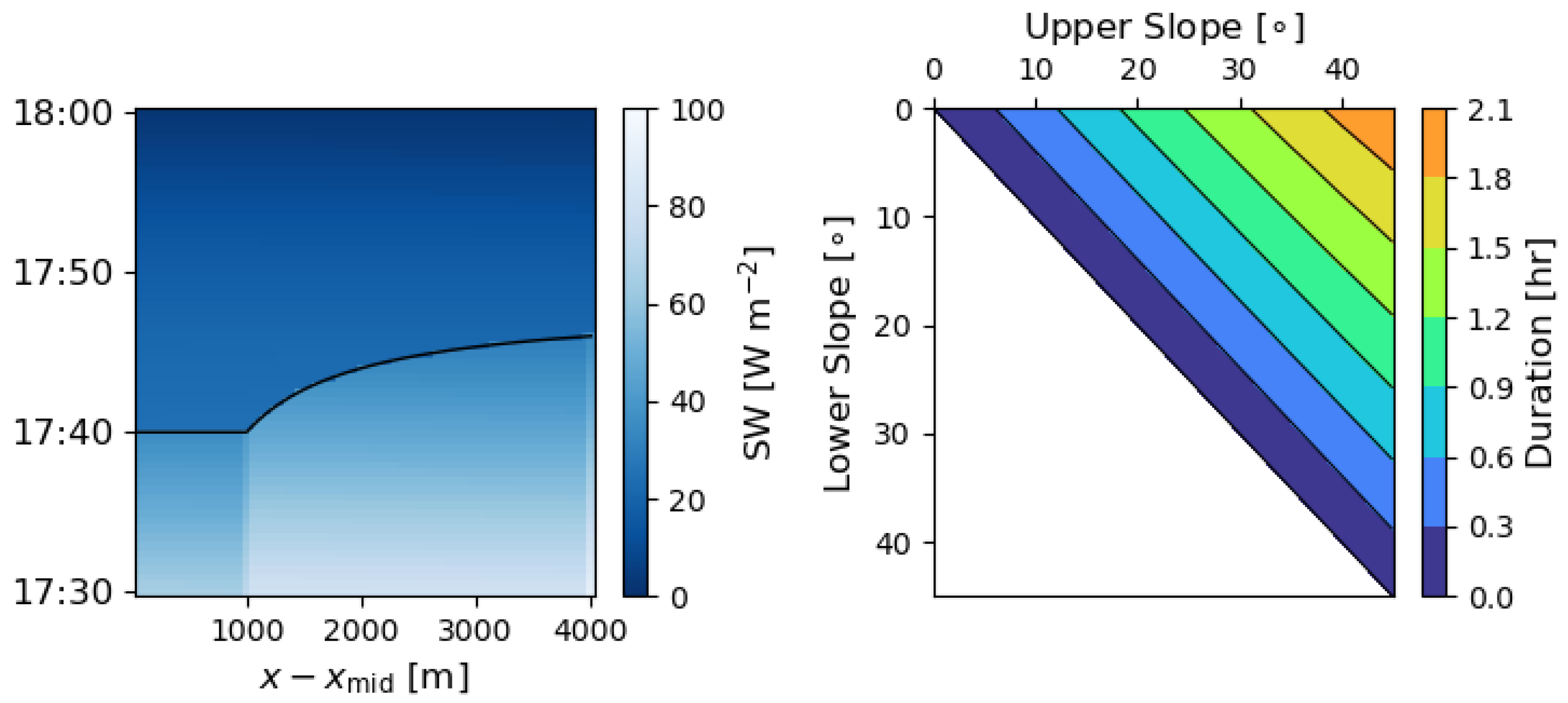
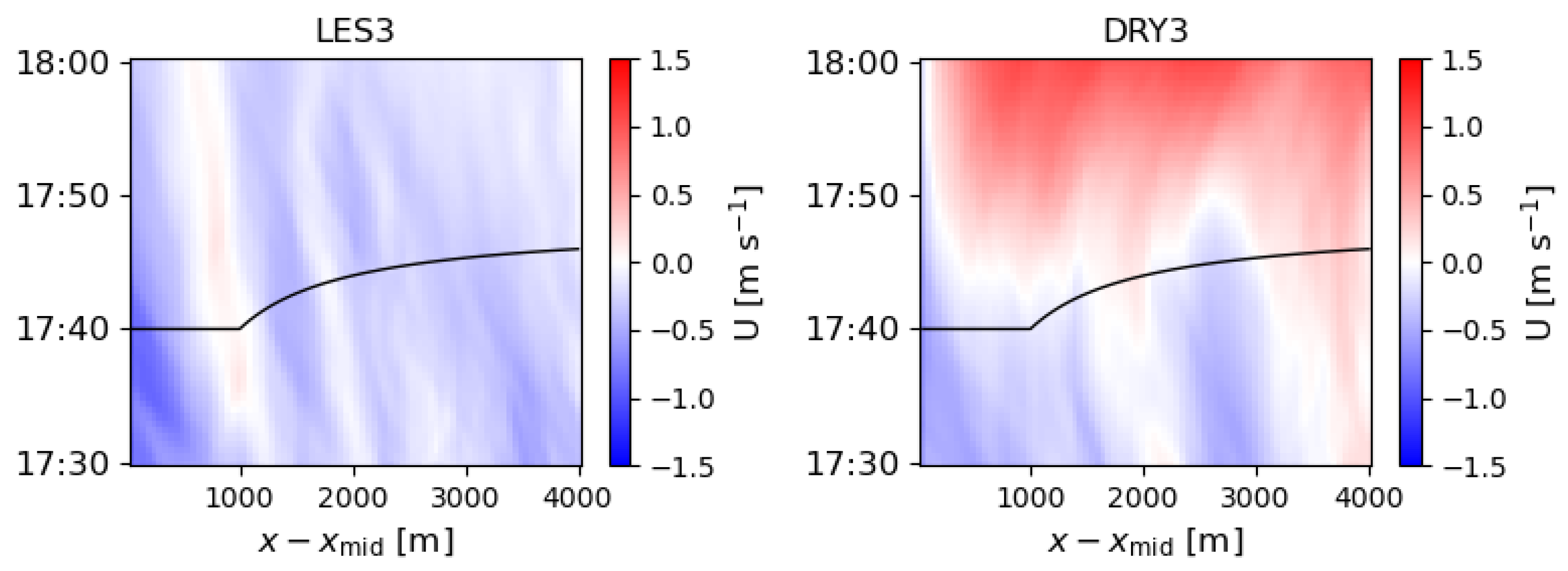
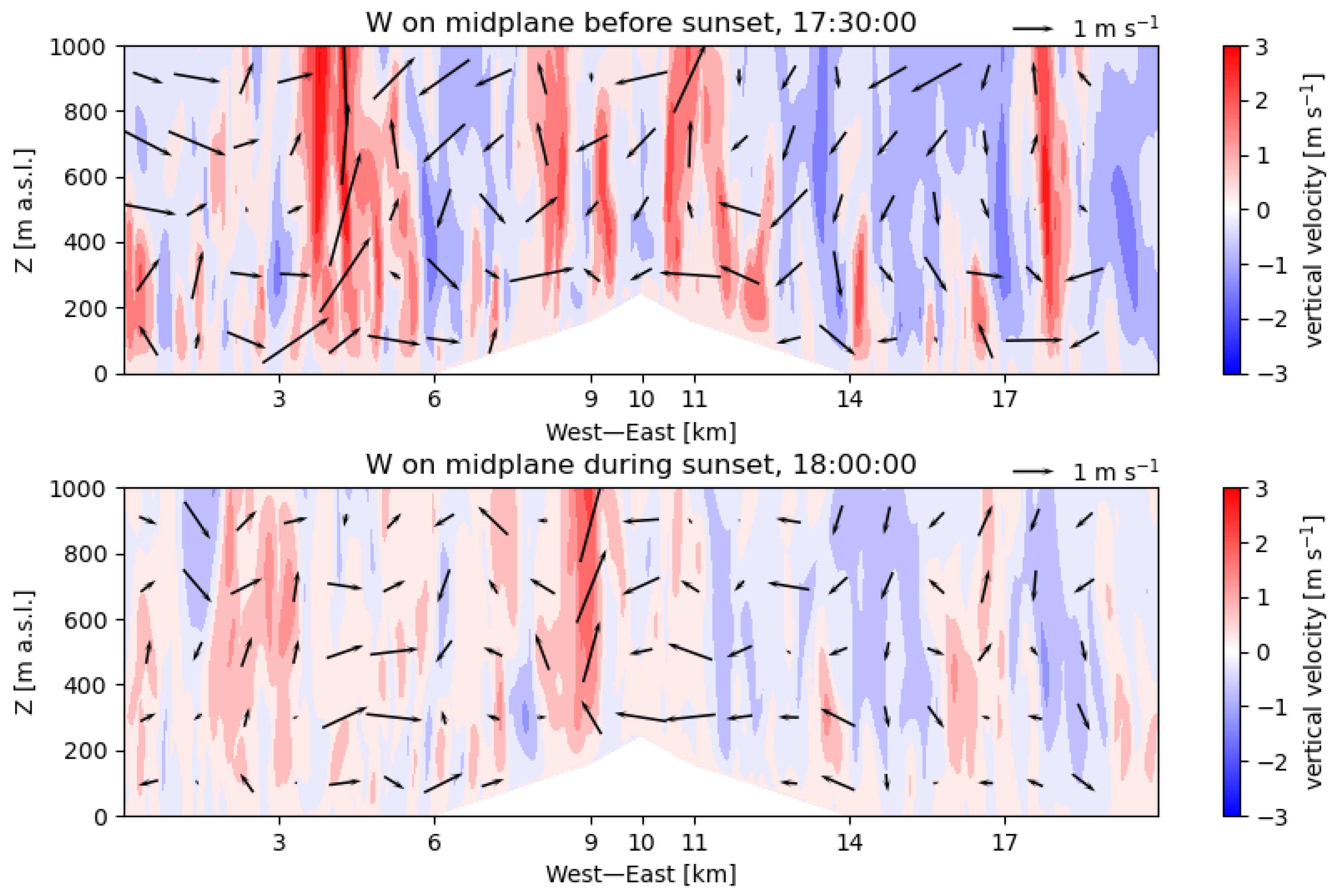
The analytical solution for the shadow front given by Equations (31) and (32) agrees quite well with the model output, manifested by a quick decrease in shortwave radiation incident on the terrain (Figure 6). The clear signal in radiation does not, however, translate to a clear signal in the x-direction velocity during the same sunset time period (Figure 7, left). While downslope flows eventually develop after sunset, the transition in LES3 (Figure 4 and Figure 5) is roughly an hour after the shadow completely encompasses the slope. Where a downslope flow is observed before sunset, $x\approx$ 11 km, it appears attributable to subsidence associated with convective structures at $x\approx$ 10.5 km and at 11.5 km (Figure 8).

This differs from the experience of Arthur et al. [10] in simulations of the onset of drainage flows with the real terrain of Granite Mountain, Utah. In their simulations, the onset of drainage flow was concurrent with—or, at some locations on the slope, even preceded—the shadow front. A possible reason for this discrepancy between the flow over the current ideal geometry and that in the real terrain used by Arthur et al. [10] is the steeper slopes, ≈${30}^{\circ }$ at the peak and ≈${15}^{\circ }$ along the foothills of Granite Mountain. Further, this ≈${15}^{\circ }$ difference between the slopes at the Granite Mountain peak and its foothills is greater than the greatest difference, $3^{\circ }$, in the slopes considered here.

A consequence of this difference in slopes is the speed of the shadow front propagating along the lower slope. We can devise a metric for the duration of sunset as a function of the dimensionless group, ${\displaystyle \frac{x-x_{\mathrm{mid}}}{L_2}}$, using Equation (31) and taking the difference in time for the shadow to reach $x-x_{\mathrm{mid}}=L_2$ and $x-x_{\mathrm{mid}}=4L_2$. This metric is plotted in the ${\varphi }_2$–${\varphi }_1$ parameter space in Figure 6 (right), where the simulations presented here, with ${\varphi }_2=5^{\circ }$ and ${\varphi }_1\in \{2^{\circ },3^{\circ },4^{\circ }\}$, occupy the upper-left corner of this diagram, among the shortest durations. For Granite Mountain, we take ${\varphi }_2\approx {30}^{\circ }$ and ${\varphi }_1\approx {15}^{\circ }$ as approximate values and arrive at predicted durations that are roughly equal to the one-hour shadow front propagation independently reported in [10].

These durations are most relevant in comparison to the timescales set by the thermal inertia of the land. We see that the land and soil characteristics are indeed important controls on this time lag given the more rapid onset seen in the DRY3 simulation. With drier soils, the transition to downslope flow occurs less than 10 min after the shadow front passes (Figure 7, right), but nowhere does a downslope flow occur before the front passage, except where attributable to convection, as in LES3. The fact that drainage flows still follow the shadow front in these 2D simulations supports the hypothesis of Arthur et al. [10], i.e., that the 3D terrain results in the early onset of a drainage flow at Granite Mountain. They argue that drainage flows can collect quickly in the narrow side valleys, which are shaded even earlier than predicted for the idealized geometry. The DRY3 simulation is missing these effects but has minimal thermal inertia. Apparently, even for longer sunset durations relative to the thermal inertia of the land, 3D effects are necessary for drainage flow onset to occur earlier than or concurrent with the shadow front.

4.3. Initial Development

An important physical process influencing the evening onset of drainage flows is daytime convection. Convective structures are shown in cross-sections of the vertical velocity taken shortly before and after the shadow front propagates along the eastern slope (Figure 8). We see that, although weakened after sunset, the same convective systems are present in similar locations as before sunset. The timescales related to the persistence of these convective structures are likely to be only weakly dependent on the slopes of the terrain but will depend strongly on the land and soil properties. Future work is needed to more systematically investigate the dependencies on the land and soil characteristics of these timescales that arise from a balance between the thermal inertia of the land surface, subject to topographic shading, and the inertia of lingering convective structures during the onset of drainage flow.

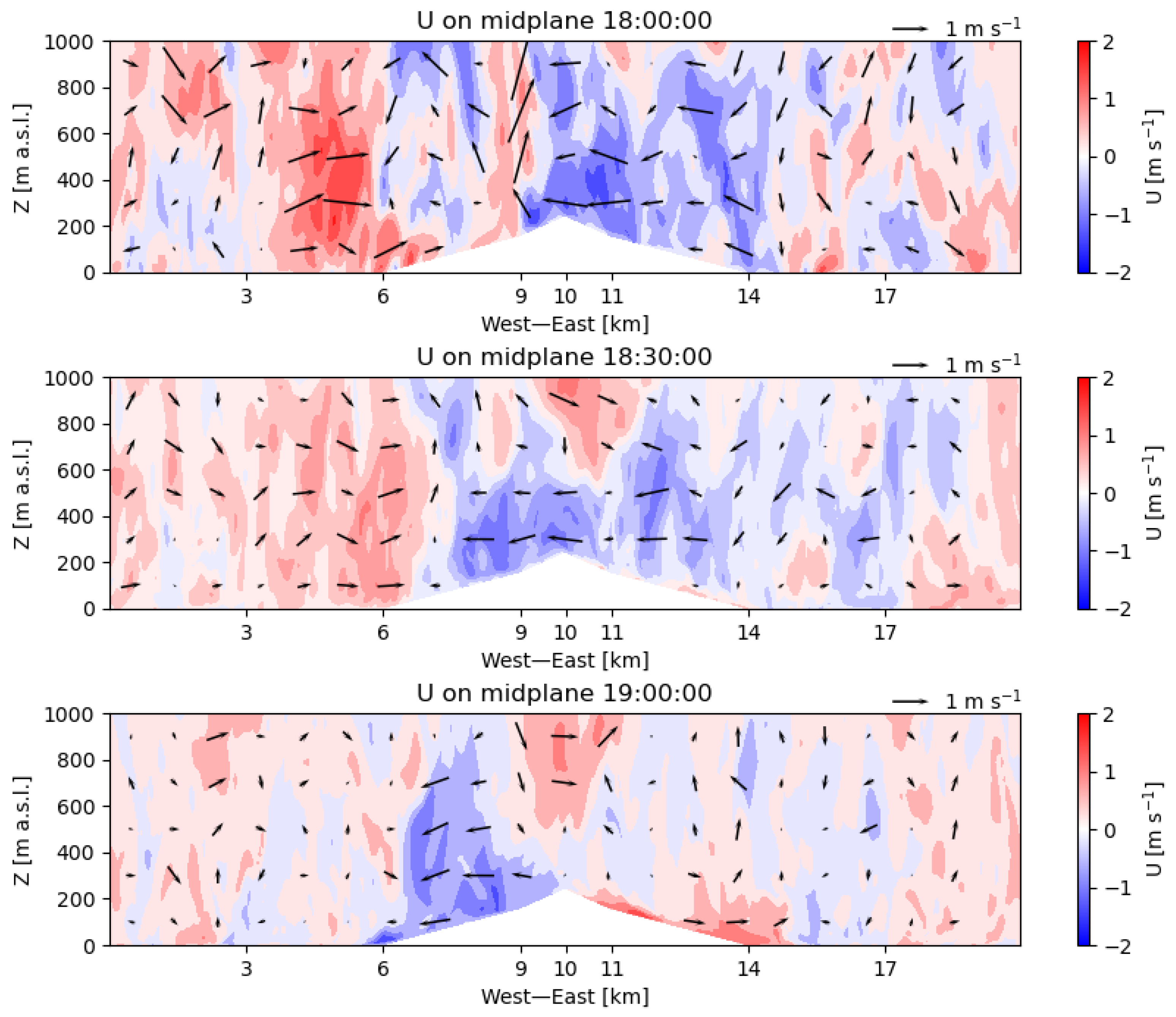
In the current simulations, the presence of convective structures post-sunset largely explains why the downslope flow initiates earlier on the sunnier western side than on the eastern slope. Because cooling by the surface boundary forces a drainage flow, this result may be counterintuitive. In Figure 9, we see horizontal convergence on the western slope at 18:00 LT (top), associated with the strong updraft near $x=$ 9 km, as also evident in the contours of the vertical velocity from the same time (Figure 8). It is reasonable to expect that such convective updrafts more often persist on the western side of the mountain because this side receives insolation for longer than the shadowy eastern side. Over the next hour (Figure 9, middle and bottom), the easterly portion of the convergent flow near the mountain peak enforces the downslope flow on the western slope, while opposing it on the eastern slope. Thus, earlier and stronger downslope flows can occur on the side that receives insolation later in the evening.

The findings at 19:30 LT, shown in Figure 10, show stronger, deeper downslope flows than are expected from buoyancy forcing alone. These initial downslope flows may be distinguished as “plunging” flows rather than “drainage” flows. Shallower drainage flows can be distinguished by 21:30, in the wakes of the plunging flows on the western slope and, on the eastern slope, colliding with the front of the easterly plunging flow, which has since passed through the periodic boundary. By 23:00, this air mass reaches the peak of the mountain, while its counterpart, the westerly plunging flow, lags behind but has similarly intruded through the periodic boundary, with its front just reaching the base of the foothills at $x=$ 6 km.

Similar intrusions repeat throughout the night, although the LESs were designed with substantial flat plains abutting the mountain slopes so that this would not occur. As such, these intrusions are arguably a shortcoming of the model. Instead of standalone simulations with periodic boundary conditions, a nested approach would address this shortcoming. A limitation of such a nested LES is the absence of resolved turbulence at the inflow from the parent mesoscale domain. With new methods for seeding turbulence tested for complex terrain cases in the WRF model [35], future work may prefer to use a nested LES strategy.

Here, our recourse is the realization that rarely do mountains exist in such isolation, so intrusions due to flows from neighboring terrain might be more typical than atypical for these wind systems. We may then decide that our model problem is most applicable to the geometry of rolling mountains or hills rather than to isolated peaks. Whether we consider these artificial or fundamental, the intrusions eventually become weak enough to study the steady-state structure of the drainage flow, as we do in the following section.

4.4. Fully Developed, Steady Drainage Flow

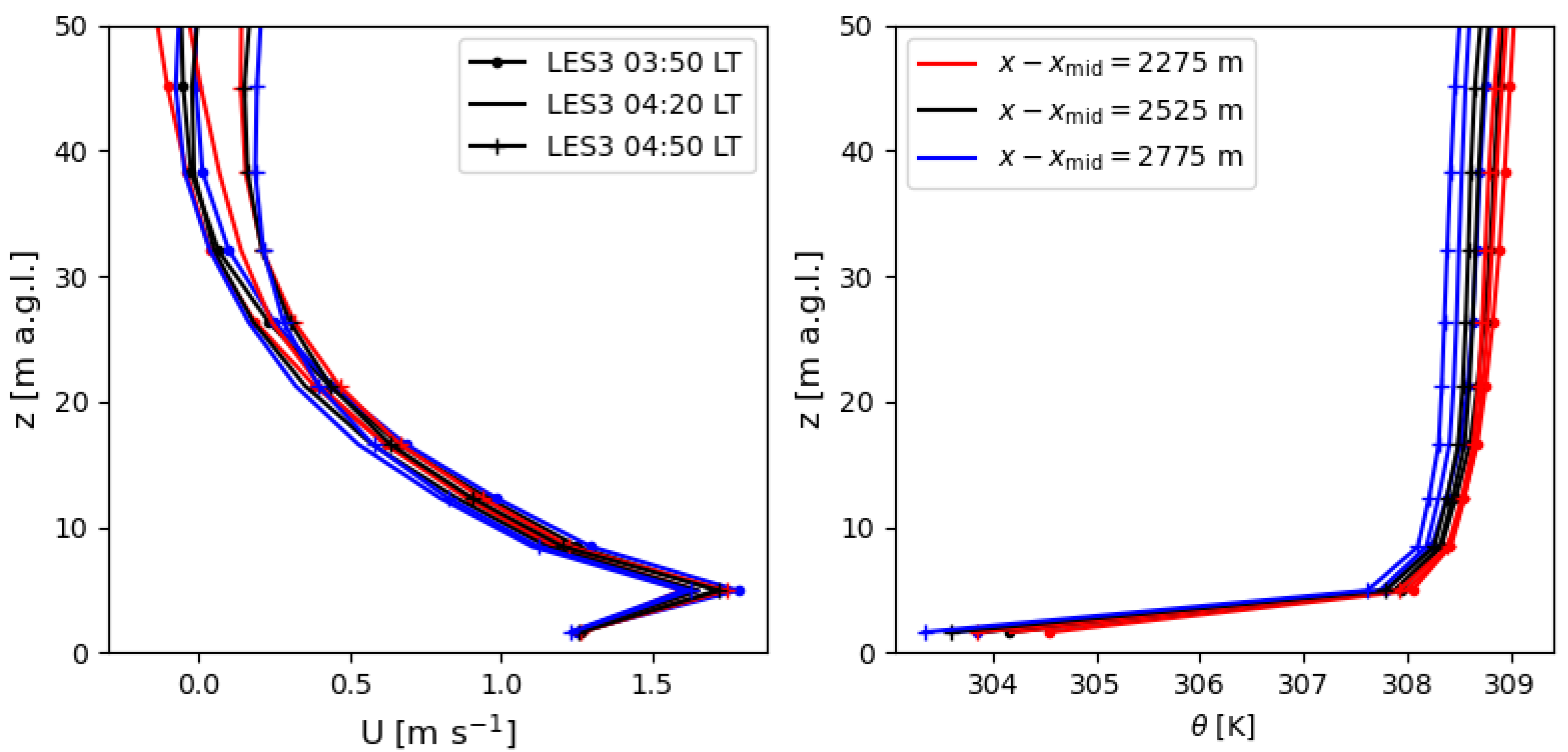
Although the initial stages of downslope flow development are complicated by both persistent convective structures and neighboring terrain, the drainage flows in the later stages of the nocturnal period are quite comparable to the steady-state, analytical solutions presented earlier (Section 2). For at least an hour, from 03:50 until 04:50, the velocity and potential temperature profiles show a steady state at the middle of the shallower eastern slope, as shown in Figure 11. During this time, the profiles of the velocity vary only slightly over 500 m, a sixth of the total slope length, centered at the middle of the slope (Figure 11). When comparing the profiles of the potential temperature, recall that the analytical solutions predict potential temperature perturbations, while the profiles in Figure 11 are of the potential temperature itself. The differences between the full temperature are consistent with stable background conditions: air farther up the slope (lower x) is warmer than lower on the slope, albeit only slightly given the shallow slopes considered here. As these profiles are similar but for a roughly constant shift, the perturbations are equal. Over the range of distances shown, the flow is therefore approximately fully developed. This time, i.e., 04:20, and this location, i.e., the middle of the shadow slope, are selected for comparisons to analytical solutions and for the investigation into the dependence on the terrain slope—a parameter that we vary for numerical experimentation.

The parameters of the analytical solutions are extracted from the LES by various means of approximation. While a rough estimate of the temperature perturbation at the surface, ${\theta }_0^{\prime }$, is relatively easy to obtain from these mean profiles, other parameters are more challenging to estimate. One challenge is that the lapse rate, $\mathrm{\Gamma }$, is not constant and has a more physically realistic profile in which stronger stability is observed nearer the surface of the plains than it is farther up the foothills (Figure 12). This feature is in part due to the drainage flows themselves, so the figure shows some differences between the LESs with varied slopes. The fact that there is no clear separation of scale between the background and slope environment exemplifies one way that the current LES is more sophisticated than previous models. It also complicates comparisons controlling for parameters other than slope in the semi-ideal setting. Despite slight differences between models, we find that approximate values from LES3, our middle slope scenario, can be applied to the other LESs, as well as being used as the parameters for the analytical solutions. From the height corresponding to the base of the steady-state profile, the LES3 results show a domain-averaged potential temperature increase of 1.5 K over 100 m. This provides a value for the background lapse rate, although no dichotomy between the background and slope environment exists in the LES. The reference temperature is similarly determined from the mean simulated temperatures (Figure 11). The parameters extracted from the LES that are used in the analytical solutions, as applicable, are

$$\begin{array}{cc}\hfill {\theta }_0^{\prime }& =-5\mathrm{K}\hfill \end{array}$$

(33)

$$\begin{array}{cc}\hfill {\theta }_0& =308\mathrm{K}\hfill \end{array}$$

(34)

$$\begin{array}{cc}\hfill \mathrm{\Gamma }& =0.015\mathrm{K}{\mathrm{m}}^{-1}\hfill \end{array}$$

(35)

$$\begin{array}{cc}\hfill g& =9.8\mathrm{m}{\mathrm{s}}^{-2}\hfill \end{array}$$

(36)

$$\begin{array}{cc}\hfill \varphi & =3^{\circ }.\hfill \end{array}$$

(37)

We estimate additional constant diffusivities

$$\begin{array}{cc}\hfill K_M& =0.015{\mathrm{m}}^2{\mathrm{s}}^{-2}\hfill \end{array}$$

(38)

$$\begin{array}{cc}\hfill K_H& =0.02{\mathrm{m}}^2{\mathrm{s}}^{-2}\hfill \end{array}$$

(39)

to compare with the Prandtl solution, as previously shown in Figure 2, from the LES results (Figure 13). In the LES, $K_M$ and $K_H$ are computed by the TKE 1.5-order turbulence closure [23,24] in WRF and vary in height. The Grisogono and Oerlemans solution allows for height variation but requires the specification of functional forms restricted by the additional requirement of a constant Prandtl number. We use the same functional form as Grisogono and Oerlemans [9] given by Equation (26), and tune the parameters below to match profiles from WRF,

$$\begin{array}{cc}\hfill C& =0.008\mathrm{m}{\mathrm{s}}^{-1}\hfill \end{array}$$

(40)

$$\begin{array}{cc}\hfill h& =20\mathrm{m}\hfill \end{array}$$

(41)

$$\begin{array}{cc}\hfill \mathrm{Pr}& =0.75,\hfill \end{array}$$

(42)

to plot the GO solution in Figure 2.

Surprisingly, although the diffusivity profiles used in the GO solution are quite similar to those predicted by the LES (Figure 13), it is not clear to which existing analytical solution the LES compares better (Figure 2). This is particularly true with regard to the height and magnitude of the velocity maximum, which occurs at approximately 5 m in the LES and Prandtl models but only about 2.5 m in the GO solution. Some of this discrepancy, however, is due to the vertical resolution in the WRF simulations, which are limited over sloped terrain [4,5] by

$$\mathsf{\Delta }z\gtrsim tan\varphi {\displaystyle \frac{\mathsf{\Delta }x}{b}}=tan{5}^{\circ }{\displaystyle \frac{50\mathrm{m}}{3}}\approx 1.5\mathrm{m},$$

(43)

This is the height of the first model half-level in our simulations. As such, the vertical resolution cannot be further refined without refining the horizontal resolution and time step, which can quickly become prohibitively expensive. The simulated wind maximum is lower magnitude than predicted by either of the analytical solutions, which are in rough agreement with each other. Farther above the jet maximum, the benefits of the variable diffusivity are apparent by the more gradual relaxation to quiescent winds, a notable feature of the LES profiles as well.

With full atmosphere and land physics, as represented by a state-of-the-art NWP parameterization suite, constant surface forcing is not a user-designated control on the flow, as in many previous LESs of drainage flows. Especially in this setting, it is not clear that a steady-state flow would fully develop over the finite slopes and finite nocturnal period simulated. Nonetheless, the LESs predict shallow jets of drainage flows. As such, even in these realistic settings, the simpler analytical work remains relevant. However, room for improvement in the analytical approach is also evident. Before undertaking model development, we present new evidence for a functional dependency on the slope angle provided by numerical experimentation in WRF-LES.

4.5. Dependence on Slope

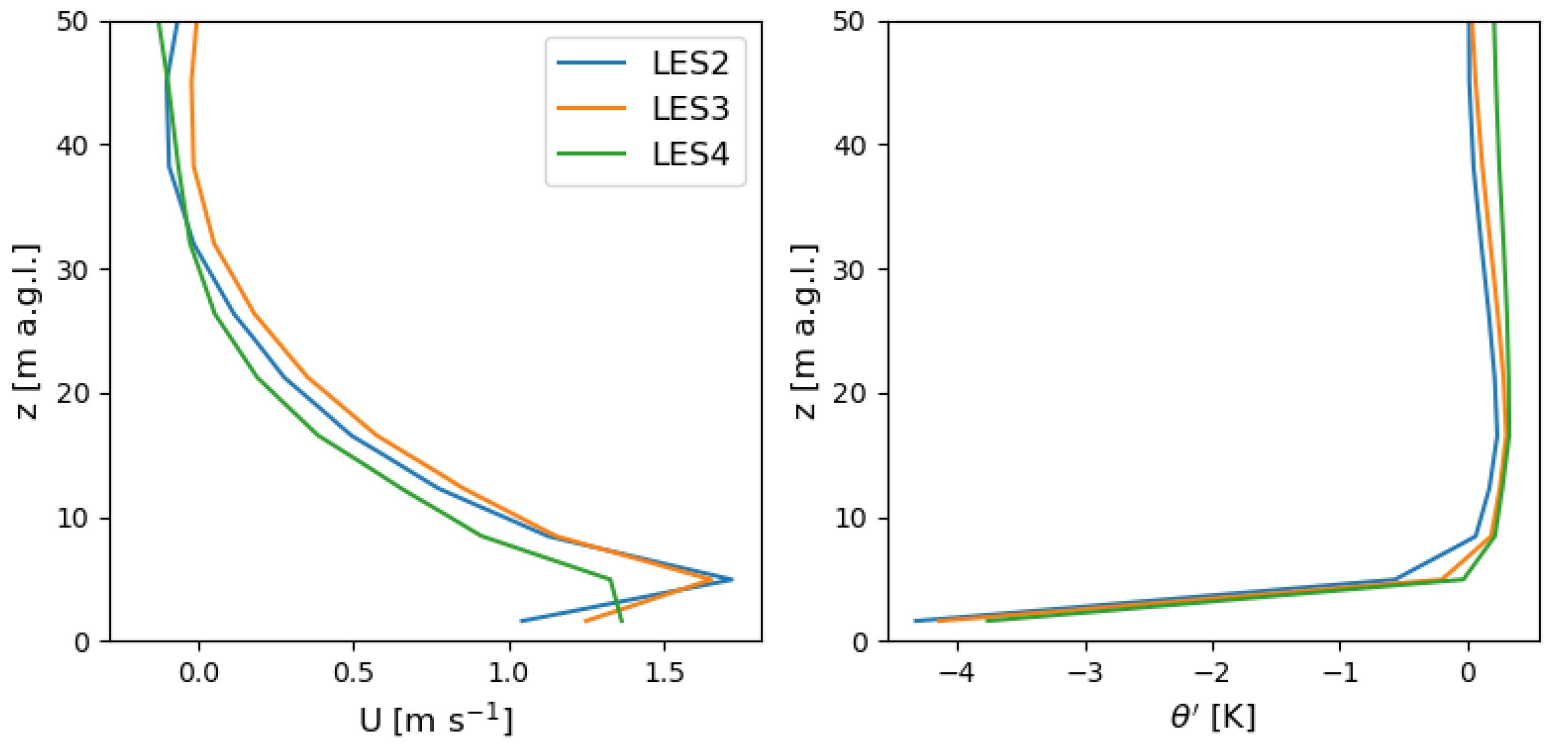
Although steeper slopes further tilt the buoyancy force vector into the along-slope direction, a more rapid decline into colder air reduces the magnitude of the buoyant force, which tends to slow the flow. Indeed, previous modeling studies of drainage flows over valley and glacier walls show that the maximum velocity, $u_{\max }$, decreases with greater slope angles [12]. This was validated indirectly through observation [11], but, in the classic Prandtl model, only the height of the velocity maximum decreases, $n_{\max }\propto 1/\sqrt{sin\varphi }$, while the magnitude is independent of the slope angle. Previous LESs corroborated $n_{\max }\propto 1/\sqrt{sin\varphi }$ but found $u_{\max }\propto 1/\sqrt{sin\varphi }$ in one study [11] and $u_{\max }\propto 1/sin\varphi$ in another [12,18]. Neither of these studies used LES coupled with advanced surface or soil parameterizations, such as those available in WRF. Importantly, even when momentum fluxes were evaluated via Monin–Obukhov similarity theory [26], either constant surface cooling or constant buoyancy fluxes (analogous to heat flux) were prescribed in previous work.

The WRF model uses a fully coupled Noah land surface model and a surface-layer scheme to jointly evaluate the fluxes of both momentum and heat, so it is worthwhile to investigate the dependence on terrain slope through the comparison of LES2, LES3, and LES4, which represent slope angles of $2^{\circ }$, $3^{\circ }$, and $4^{\circ }$, respectively. Complicating this effort to isolate the direct influence of the slope angle are a number of secondary effects that respond to changes in slope. Although the radiative fluxes, which dominate the regional energy balance, are only slightly altered in this small range of angles, from two degrees to four degrees, the presence of the drainage flows themselves affects the background thermal structure (Figure 12). Nonetheless, the same lapse rate used in the analytical models does well to remove the background in the potential temperature profiles shown in Figure 14 for all of the LESs compared. However, we reduce the potential temperature to its perturbation by subtracting a reference that is 0.25 K lower for LES2 than the ${\theta }_0$ of 308 K found in the other LESs.

The velocity profiles in the current LES show that the velocity maximum decreases with increasing slope angles (Figure 14), as in more idealized LESs [11,12,18]. Here, the relatively coarse vertical resolution and sparse coverage of incline angles preclude a meaningful statistical fit to $sin\varphi$, especially for the height of the jet maximum. Qualitatively, we can determine that the current LESs agree with the previous LESs in that the highest slope angles result in the shallowest jets. For a more satisfactory description of the vertical structure, future work may iterate on the estimates of the jet height shown here to act on the advice of Smith and Porté-Agel [7] to improve LES by placing additional grid levels below the jet height.

4.6. The Flux–Prandtl Solution

The lack of dependence of the wind maximum on the slope angle is a much discussed discrepancy between Prandtl’s analytical model and simulations [11,18]. In the same physical setting as Prandtl, we present a new analytical solution that explains this.

To derive this Flux–Prandtl solution, we retain all the assumptions of Prandtl, including that of constant eddy diffusivities (Section 2.1). Instead of a constant temperature deficiency, we assign a constant temperature flux, $\overline{w^{\prime }{\theta }^{\prime }}$, at the bottom surface as a Neumann boundary condition:

$${\displaystyle \frac{\partial {\theta }^{\prime }}{\partial n}}{|}_{n=0}={\displaystyle \frac{-\overline{w^{\prime }{\theta }^{\prime }}}{K_H}}$$

(44)

For this system (Equations (3) and (4)), subject to these new boundary conditions, the solution is based on the complex exponential, $F=exp[-(1+i\left)\sigma n\right]$, given in Equation (13):

$$\begin{array}{cc}\hfill u=-& {\displaystyle \frac{\overline{w^{\prime }{\theta }^{\prime }}}{\sigma K_H}}\mu Im\left(F\right)=-{\displaystyle \frac{\overline{w^{\prime }{\theta }^{\prime }}}{\sqrt{K_H}}}{\left({\displaystyle \frac{{\sigma }_0}{2}}\right)}^{-1/2}\mu Im\left(F\right)\hfill \end{array}$$

(45)

$$\begin{array}{cc}\hfill {\theta }^{\prime }=& {\displaystyle \frac{\overline{w^{\prime }{\theta }^{\prime }}}{\sigma K_H}}Re\left(F\right)={\displaystyle \frac{\overline{w^{\prime }{\theta }^{\prime }}}{\sqrt{K_H}}}{\left({\displaystyle \frac{{\sigma }_0}{2}}\right)}^{-1/2}Re\left(F\right)\hfill \end{array}$$

(46)

where

$$\begin{array}{cc}\hfill \sigma & ={\left({\displaystyle \frac{g\mathrm{\Gamma }{sin}^2\varphi }{4{\theta }_0{K}_M{K}_H}}\right)}^{{\displaystyle \frac{1}{4}}}\left[{\mathrm{m}}^{-1}\right],{\sigma }_0^2={\displaystyle \frac{g\mathrm{\Gamma }{sin}^2\varphi }{{\theta }_{0}Pr}}\left[{\mathrm{s}}^{-2}\right]\hfill \end{array}$$

(47)

$$\begin{array}{cc}\hfill \mu & ={\left({\displaystyle \frac{g{K}_H}{{\theta }_0\mathrm{\Gamma }{K}_M}}\right)}^{{\displaystyle \frac{1}{2}}}={\left({\displaystyle \frac{g}{{\theta }_0\mathrm{\Gamma }\mathrm{Pr}}}\right)}^{{\displaystyle \frac{1}{2}}}\left[\mathrm{m}{\mathrm{s}}^{-1}{\mathrm{K}}^{-1}\right].\hfill \end{array}$$

(48)

In this abbreviated form, it is easiest to see that the Prandtl solution can be recovered with the substitution

$${\theta }_0^{\prime }={\displaystyle \frac{\overline{w^{\prime }{\theta }^{\prime }}}{\sigma K_H}}={\displaystyle \frac{\overline{w^{\prime }{\theta }^{\prime }}}{\sqrt{K_H}}}{\left({\displaystyle \frac{{\sigma }_0}{2}}\right)}^{-1/2}.$$

(49)

With constant diffusivities, as in the original Prandtl model, the dependency on the slope of the height of the wind maximum is unchanged with a heat flux boundary condition. However, in this case, the magnitude of the wind velocity maximum inherits the same dependency on the slope from $\sigma$ for

$$\begin{array}{ccc}\hfill n_{\max }& ={\displaystyle \frac{\pi }{4}}{\sigma }^{-1}\hfill & \hfill \propto 1/\sqrt{sin\varphi }\end{array}$$

(50)

$$\begin{array}{ccc}\hfill u_{\max }& =-{\displaystyle \frac{\overline{w^{\prime }{\theta }^{\prime }}}{\sigma K_H}}{e}^{{\displaystyle \frac{-\pi }{4}}}{\displaystyle \frac{\sqrt{2}}{2}}\hfill & \hfill \propto 1/\sqrt{sin\varphi }.\end{array}$$

(51)

Holding other parameters constant, $u_{\max }$ does decrease over steeper slopes when replacing the Dirichlet boundary conditions with Neumann boundary conditions in the original Prandtl model. The fact that previous LES used boundary conditions that were more similar to these flux conditions explains the discrepancy with the Prandtl model, but only when enforcing Dirichlet conditions. With surface heat flux applied as a Neumann boundary condition, the Prandtl model recreates the same power law found by a previous numerical experiment [11], which is qualitatively similar to others [18], including the current, in which the velocity maximum decreases with increasing slope angles (Figure 14).

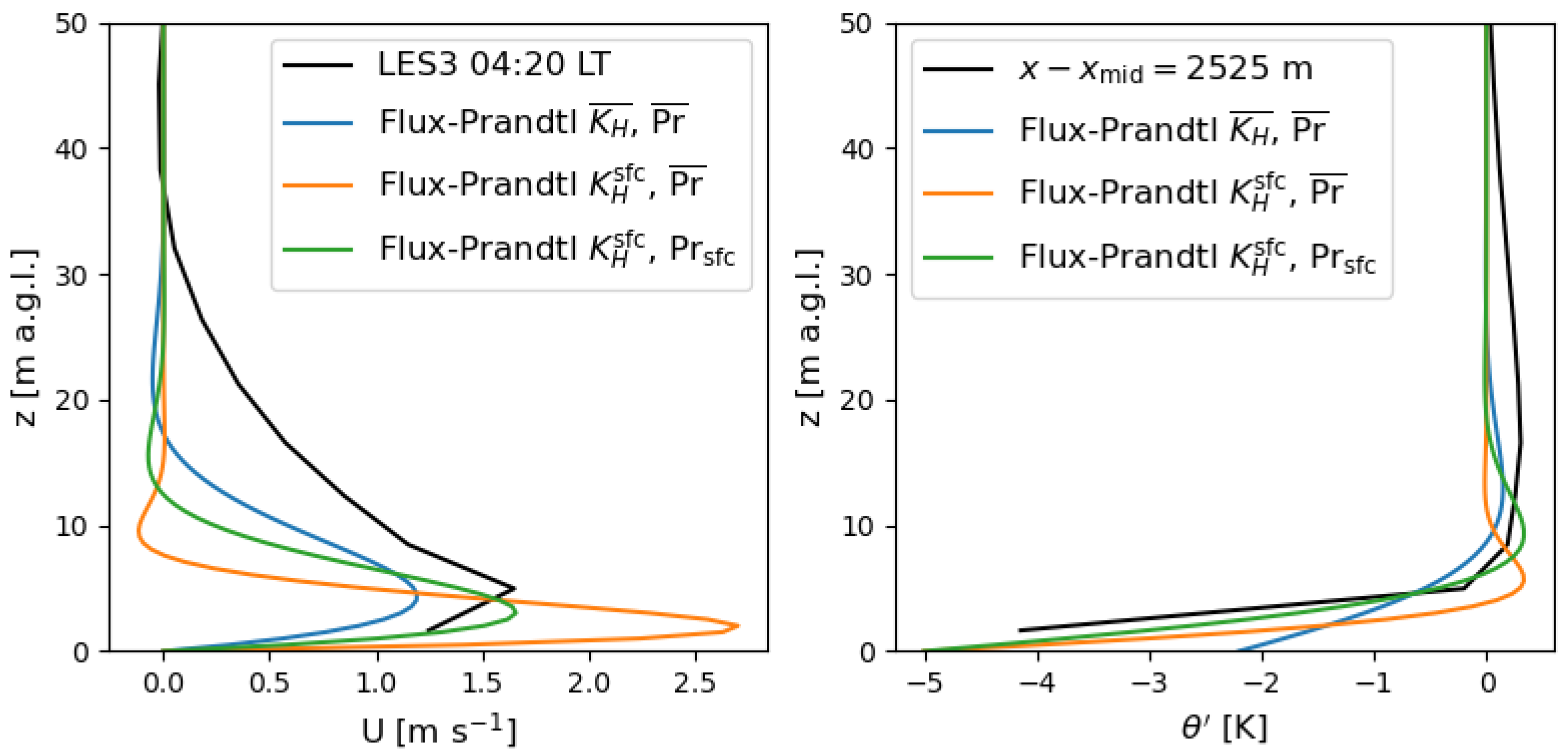
As with the other parameters, we take the surface heat flux, $\overline{w^{\prime }{\theta }^{\prime }}$ = −0.008 K m $s^{-1}$, from WRF-LES. However, the resulting solutions in Figure 15 (blue) improve the agreement only in the velocity, while severely underestimating the temperature deficit at the surface. We can instead choose to parameter-fit both the temperature flux at the surface and the perturbation itself there. From Equation (49), we define an effective eddy diffusivity at the surface,

$$K_H^{\mathrm{sfc}}={\left({\displaystyle \frac{\overline{w^{\prime }{\theta }^{\prime }}}{{\theta }_0^{\prime }}}\right)}^2{\left({\displaystyle \frac{{\sigma }_0}{2}}\right)}^{-1}$$

(52)

In such a case, the dependency on the slope is altered,

$$\begin{array}{ccc}\hfill n_{\max }& ={\displaystyle \frac{\pi }{4}}{\displaystyle \frac{\overline{w^{\prime }{\theta }^{\prime }}}{{\theta }_0^{\prime }}}{\left({\displaystyle \frac{{\sigma }_0}{2}}\right)}^{-1}\hfill & \hfill \propto 1/sin\varphi \end{array}$$

(53)

$$\begin{array}{ccc}\hfill u_{\max }& ={\theta }_0^{\prime }\mu e^{{\displaystyle \frac{-\pi }{4}}}{\displaystyle \frac{\sqrt{2}}{2}}\hfill & \hfill \propto {(sin\varphi )}^0\end{array}$$

(54)

while the agreement with the temperature perturbation at the surface is much improved (Figure 15, orange and green).

With comparable Prandtl numbers, the effective surface diffusivity is about an order of magnitude lower than those used previously to characterize full profiles from the LES (Figure 13). As in the GO solution with Pr = 0.75 (Figure 2), which had the diffusivities approach zero at the surface, the newly predicted jet (Figure 15, orange) is lower and its magnitude increased. This is a consequence of fitting the diffusivities to the surface but not adjusting the Prandtl number. We note that, in WRF (Figure 13), not only do the diffusivities decrease near the surface but the Prandtl number increases. This is consistent with a known dependency of the turbulent Prandtl number on density stratification, typically as a function of the Richardson number for stable cases [36]. As the near-surface temperature gradients here are large, we may expect a larger Prandtl number, ${\mathrm{Pr}}_{\mathrm{sfc}}$ = 2, to better represent this strongly stable surface layer. When we adjust both these parameters (Figure 15, green), the velocity maximum agrees better and the height of the jet returns to roughly that of the LES. However, although the jet deepens, it remains relatively symmetric compared to GO or LES, because the diffusivities are held constant at a low surface value, which inhibits mixing momentum farther above the jet height.

4.7. The Flux–GO Solution

The parameters for the diffusivity profiles used in the GO solution given by Equation (26) were selected based on comparisons to those from LES3 (Figure 13). Instead, we may abandon this fidelity approach and choose to define an effective eddy diffusivity that will take non-zero values at the surface, such that solutions fit to surface flux values may be physically consistent. We blend the two with a relatively simple combination

$$K_H^{\mathrm{eff}}=K_H^{\mathrm{sfc}}+a·K_H^{\mathrm{GO}}$$

(55)

with $a={\displaystyle \frac{1}{2}}$ and we plot in Figure 16 the Flux–GO solutions as

$$\begin{array}{cc}\hfill F& =exp\left[-(1+i){\left({\sigma }_0/2\right)}^{1/2}{\int }_0^n{\left(K_H^{\mathrm{eff}}\right)}^{-{\displaystyle \frac{1}{2}}}d{n}^{\prime }\right]\hfill \end{array}$$

(56)

$$\begin{array}{cc}\hfill u& =-{\displaystyle \frac{\overline{w^{\prime }{\theta }^{\prime }}}{\sqrt{K_H^{\mathrm{sfc}}}}}{\left({\displaystyle \frac{{\sigma }_0}{2}}\right)}^{-1/2}\mu Im\left(F\right)\hfill \end{array}$$

(57)

$$\begin{array}{cc}\hfill {\theta }^{\prime }& ={\displaystyle \frac{\overline{w^{\prime }{\theta }^{\prime }}}{\sqrt{K_H^{\mathrm{sfc}}}}}{\left({\displaystyle \frac{{\sigma }_0}{2}}\right)}^{-1/2}Re\left(F\right)\hfill \end{array}$$

(58)

which, as with the Flux–Prandtl cases, agrees with LES best when the turbulent Prandtl number is increased to reflect the near-surface values. In this case, the magnitude and height of the jet are well approximated, and the more gradual relaxation to quiescent winds is also represented.

The need for a non-zero diffusivity at the surface naturally extends to this effective diffusivity approach, but the impact of a non-constant Prandtl number is not addressed. Although the LES resolves variations in the Prandtl number (Figure 13), we have selected an even larger Prandtl number to more dramatically demonstrate the effect of the Prandtl number on the shape of the profile. We argue that this represents the unresolved surface layer, so this choice unsurprisingly leads to improved agreement at and below the jet height. However, disagreement above jet heights where the Prandtl number is less representative remains. We understand this to be a consequence of larger diffusivities, which are a function of the Prandtl number (Equation (52)). In the velocity profiles, this is a benefit because the WRF profiles also exhibit more gradual relaxation to quiescent winds. In the temperature profiles, however, the gradual relaxation to a reference temperature is less physical. We did not attempt to optimize our combination of the diffusivities at the surface, $K_H^{\mathrm{sfc}}$, and above, $K_H^{\mathrm{GO}}$, from the GO solution. For instance, specifying the fraction, a, in Equation (55) as a function of Pr to counteract the Pr dependence in Equation (52) could further improve the agreement of the Flux–GO solution with the LES. However, because this thermal diffusivity does not decrease relative to the momentum, the relatively sharp gradients in temperature appear irreconcilable with the gradual relaxation to quiescent winds in lieu of a variable Prandtl number.

Further extension of the current analytical model could revisit the WKB method and instead take Pr as the parameter that varies the momentum diffusivities relative to a fixed heat diffusivity, fit to the surface flux values. Alternatively, absorbing the Prandtl number dependence into integrals analogous to those in Equation (20) may account for the joint variability in eddy diffusivities and their ratio, the turbulent Prandtl number. More tangentially, a momentum surface flux can be enforced with the same governing equations, similarly to the surface heat flux considered here. Such analytical work should be encouraged by the agreement with LES achieved through the model developments presented here.

5. Conclusions

To improve the understanding and analytical modeling of drainage flows, we performed large-eddy simulations in the WRF model. In our semi-idealized setting, realistic radiation forces a fully coupled land surface model in simulations with an idealized compound-slope mountain topography (Figure 3). The mean flow is characterized by symmetry inherited from this simple surface geometry through the majority of the diurnal cycle (Figure 4 and Figure 5). At sunset, topographic shading alters the radiative forcing and induces asymmetry. An analysis of this period in the semi-ideal model allows both an analytical description of the mountain shadow (Figure 6) and the resolution of complex convective structures that respond to these radiation patterns (Figure 8). Horizontal convergence associated with the convective structures explains the onset of stronger downslope flows earlier on the sunnier, western side (Figure 9). This counterintuitive result indicates that care is needed when interpreting downslope flows during the evening transition, where background flow conditions including convective structures may influence the flow.

The relation of the shadow front and the development of downslope flows in the LES is strongly influenced by the thermal inertia of the land, which is sensitive to soil moisture in the current simulations (Figure 7). Flow from neighboring terrain—here, flow through the periodic boundaries—also affects the development of downslope flows (Figure 10). The influence of such phenomena, and of three-dimensional terrain effects [10], which were absent in the current LES, should be considered during the early nocturnal period.

In our compound-slope mountain setup, approximately fully developed steady drainage flows appeared in the LES late in the nocturnal period (Figure 11). During this period, parameters were extracted from WRF and used in analytical models. Novel analytical solutions, namely the Flux–Prandtl (Equations (45)–(48)) and Flux–GO solutions (Equations (56)–(58)), were derived by applying Neumann boundary conditions that were physically consistent with the surface heat flux in the LES. Without further modification to the Prandtl model, the flux-based solution recreates the flow dependence on slope that was previously reported [11], which is qualitatively similar to that seen in other work [18] and the current LES (Figure 14).

Variants of this new analytical solution illustrate the effects on the predicted profiles of various strategies to specify the diffusivity and turbulent Prandtl number (Figure 15 and Figure 16). These show that models of drainage flow are improved by resolving the disconnection between surface processes and turbulent processes in the stable atmospheric boundary layer above. In the LES, the staggered discrete grid allows some finite depth over which fluxes at the surface are inferred from flux–gradient relationships that differ from the eddy diffusivity model used elsewhere. In the analytical setting, there is no discrete grid to separate the surface physics. Instead, we alter the eddy diffusivity to fit to surface parameters while retaining the convenient form of a down-gradient flux with an effective eddy diffusivity approach (Equation (55)). Contributing to the effective diffusivity is the non-zero value required to fit both the surface heat flux and temperature perturbation at the surface (Equation (52)). This is added to a fraction of the original GO formulations (Equation (26)) with parameters fit to the LES (Figure 13).

Improving the analytical model’s fidelity to near-surface dynamics leads to further improvements in predictions of the jet height and velocity maximum (Figure 16) when selecting larger turbulent Prandtl numbers expected from the strong near-surface stability. The LES results resolve such a vertical structure in the Prandtl number, consistent with the dynamics of stably stratified flows (Figure 13). However, even in the new analytical models, restriction to a constant Prandtl number remains a source of error. Future analytical work may consider how to best model drainage flows with variable Prandtl numbers and may benefit from information provided by an advanced NWP, as described here. The analytical solutions proposed here ingest the surface heat flux, provided by WRF-LES, and are improved by adopting the effective eddy diffusivity necessary to enforce flux boundary conditions in analytical models of drainage flows.

References

1. Lareau, N.P.; Crosman, E.; Whiteman, C.D.; Horel, J.D.; Hoch, S.W.; Brown, W.O.; Horst, T.W. The persistent cold-air pool study. Bull. Am. Meteorol. Soc. 2013, 94, 51–63. [Google Scholar] [CrossRef]
2. Holden, Z.A.; Jolly, W.M. Modeling topographic influences on fuel moisture and fire danger in complex terrain to improve wildland fire management decision support. For. Ecol. Manag. 2011, 262, 2133–2141. [Google Scholar] [CrossRef]
3. Massey, J.D.; Steenburgh, W.J.; Knievel, J.C.; Cheng, W.Y. Regional soil moisture biases and their influence on WRF model temperature forecasts over the intermountain west. Weather Forecast. 2016, 31, 197–216. [Google Scholar] [CrossRef]
4. Connolly, A.; Chow, F.K.; Hoch, S.W. Nested large-eddy simulations of the displacement of a cold-air pool by lee vortices. Bound.-Layer Meteorol. 2021, 178, 91–118. [Google Scholar] [CrossRef]
5. Mahrer, Y. An improved numerical approximation of the horizontal gradients in a terrain-following coordinate system. Mon. Weather Rev. 1984, 112, 918–922. [Google Scholar] [CrossRef]
6. Bouëdec, E.L.; Chemel, C.; Staquet, C. Dealing with steep slopes when modeling stable boundary-layer flow in Alpine terrain. Q. J. R. Meteorol. Soc. 2025, 151, e4835. [Google Scholar] [CrossRef]
7. Smith, C.M.; Porté-Agel, F. An intercomparison of subgrid models for large-eddy simulation of katabatic flows. Q. J. R. Meteorol. Soc. 2014, 140, 1294–1303. [Google Scholar] [CrossRef]
8. Prandtl, L. Führer Durch die Strömungslehre (Essentials of Fluid Mechanics); Vieweg und Sohn: Braunschweig (Brunswick), Germany, 1942. [Google Scholar]
9. Grisogono, B.; Oerlemans, J. Katabatic flow: Analytic solution for gradually varying eddy diffusivities. J. Atmos. Sci. 2001, 58, 3349–3354. [Google Scholar] [CrossRef]
10. Arthur, R.S.; Lundquist, K.A.; Mirocha, J.D.; Chow, F.K. Topographic effects on radiation in the WRF Model with the immersed boundary method: Implementation, validation, and application to complex terrain. Mon. Weather Rev. 2018, 146, 3277–3292. [Google Scholar] [CrossRef]
11. Grisogono, B.; Axelsen, S.L. A note on the pure katabatic wind maximum over gentle slopes. Bound.-Layer Meteorol. 2012, 145, 527–538. [Google Scholar] [CrossRef]
12. Axelsen, S.; Dop, H. Large-eddy simulation of katabatic winds. Part 1: Comparison with observations. Acta Geophys. 2009, 57, 803–836. [Google Scholar] [CrossRef]
13. Defant, F. Zur theorie der Hangwinde, nebst Bemerkungen zur Theorie der Berg-und Talwinde. Arch. Meteorol. Geophys. Bioklimatol. Ser. A 1949, 1, 421–450. [Google Scholar] [CrossRef]
14. Manins, P.; Sawford, B. A model of katabatic winds. J. Atmos. Sci. 1979, 36, 619–630. [Google Scholar] [CrossRef]
15. Mahrt, L. Momentum balance of gravity flows. J. Atmos. Sci. 1982, 39, 2701–2711. [Google Scholar] [CrossRef]
16. Horst, T.; Doran, J. Nocturnal drainage flow on simple slopes. Bound.-Layer Meteorol. 1986, 34, 263–286. [Google Scholar] [CrossRef]
17. Egger, J. Thermally forced flows: Theory. In Atmospheric Processes over Complex Terrain; American Meteorological Society: Boston, MA, USA, 1990; pp. 43–58. [Google Scholar]
18. Axelsen, S.; Dop, H. Large-eddy simulation of katabatic winds. Part 2: Sensitivity study and comparison with analytical models. Acta Geophys. 2009, 57, 837–856. [Google Scholar] [CrossRef]
19. Wood, N. Wind flow over complex terrain: A historical perspective and the prospect for large-eddy modelling. Bound.-Layer Meteorol. 2000, 96, 11–32. [Google Scholar] [CrossRef]
20. Chow, F.K.; De Wekker, S.F.; Snyder, B.J. (Eds.) Mountain Weather Research and Forecasting: Recent Progress and Current Challenges; Springer: New York, NY, USA, 2013. [Google Scholar]
21. Smith, C.M.; Skyllingstad, E.D. Numerical simulation of katabatic flow with changing slope angle. Mon. Weather Rev. 2005, 133, 3065–3080. [Google Scholar] [CrossRef]
22. Schmidli, J.; Billings, B.; Chow, F.K.; de Wekker, S.F.; Doyle, J.; Grubišić, V.; Holt, T.; Jiang, Q.; Lundquist, K.A.; Sheridan, P.; et al. Intercomparison of mesoscale model simulations of the daytime valley wind system. Mon. Weather Rev. 2011, 139, 1389–1409. [Google Scholar] [CrossRef]
23. Moeng, C.H. A large-eddy-simulation model for the study of planetary boundary-layer turbulence. J. Atmos. Sci. 1984, 41, 2052–2062. [Google Scholar] [CrossRef]
24. Moeng, C.; Dudhia, J.; Klemp, J.; Sullivan, P. Examining two-way grid nesting for large eddy simulation of the PBL using the WRF model. Mon. Weather Rev. 2007, 135, 2295–2311. [Google Scholar] [CrossRef]
25. Chen, F.; Janjić, Z.; Mitchell, K. Impact of atmospheric surface-layer parameterizations in the new land-surface scheme of the NCEP mesoscale Eta model. Bound.-Layer Meteorol. 1997, 85, 391–421. [Google Scholar] [CrossRef]
26. Monin, A.S.; Obukhov, A.M. Basic laws of turbulent mixing in the surface layer of the atmosphere. Contrib. Geophys. Inst. Acad. Sci. USSR 1954, 151, e187. [Google Scholar]
27. Chenge, Y.; Brutsaert, W. Flux-profile relationships for wind speed and temperature in the stable atmospheric boundary layer. Bound.-Layer Meteorol. 2005, 114, 519–538. [Google Scholar] [CrossRef]
28. Jiménez, P.A.; Dudhia, J.; González-Rouco, J.F.; Navarro, J.; Montávez, J.P.; García-Bustamante, E. A revised scheme for the WRF surface layer formulation. Mon. Weather Rev. 2012, 140, 898–918. [Google Scholar] [CrossRef]
29. Mlawer, E.J.; Taubman, S.J.; Brown, P.D.; Iacono, M.J.; Clough, S.A. Radiative transfer for inhomogeneous atmospheres: RRTM, a validated correlated-k model for the longwave. J. Geophys. Res. Atmos. 1997, 102, 16663–16682. [Google Scholar] [CrossRef]
30. Dudhia, J. Numerical study of convection observed during the winter monsoon experiment using a mesoscale two-dimensional model. J. Atmos. Sci. 1989, 46, 3077–3107. [Google Scholar] [CrossRef]
31. Zängl, G. Formation of extreme cold-air pools in elevated sinkholes: An idealized numerical process study. Mon. Weather Rev. 2005, 133, 925–941. [Google Scholar] [CrossRef]
32. Chen, F.; Dudhia, J. Coupling an advanced land surface-hydrology model with the Penn State-NCAR MM5 modeling system. Part I: Model implementation and sensitivity. Mon. Weather Rev. 2001, 129, 569–585. [Google Scholar] [CrossRef]
33. Skamarock, W.C.; Klemp, J.B.; Dudhia, J.; Gill, D.O.; Barker, D.M.; Wang, W.; Powers, J.G. A Description of the Advanced Research WRF Version 3; Technical report; NCAR: Boulder, CO, USA, 2008. [Google Scholar]
34. Zardi, D.; Whiteman, C.D. Diurnal Mountain Wind Systems. In Mountain Weather Research and Forecasting: Recent Progress and Current Challenges; Chow, F.K., De Wekker, S.F., Snyder, B.J., Eds.; Springer: Dordrecht, The Netherlands, 2013; pp. 35–119. [Google Scholar] [CrossRef]
35. Connolly, A.; van Veen, L.; Neher, J.; Geurts, B.J.; Mirocha, J.; Chow, F.K. Efficacy of the cell perturbation method in large-eddy simulations of boundary layer flow over complex terrain. Atmosphere 2021, 12, 55. [Google Scholar] [CrossRef]
36. Katul, G.G.; Porporato, A.; Shah, S.; Bou-Zeid, E. Two phenomenological constants explain similarity laws in stably stratified turbulence. Phys. Rev. E 2014, 89, 023007. [Google Scholar]
Figure 1. Illustration of rotated coordinates and variables in the setting of the considered analytical solutions for drainage flow. The solid slope surface is black with hatches and the blue lines are levels in a vertical, not slope-normal, temperature gradient.
Atmosphere 16 01091 g001
Figure 2. Analytical solutions of drainage flows from Prandtl and from Grisogono and Oerlemans (GO), both using ϕ = 3 , θ 0 = −5 K, θ 0 = 308 K, Γ = 0.015 K m 1 , and g = 9.8 m s 2 , compared to those during a steady, fully developed flow in LES3. Diffusivities in the Prandtl solution are constants, K M = 0.015 m 2 s 1 , K H = 0.02 m 2 s 1 , while the GO solution uses Pr = 0.75 and K M given by Equation (26).
Atmosphere 16 01091 g002
Figure 3. Illustration of the 2D compound-slope mountain geometry that defines the LES topography.
Atmosphere 16 01091 g003
Figure 4. Hovmöller diagram of x-direction velocity at the first model half-level, ≈1.5 m a.g.l., averaged in the south–north direction from LES3 for the entire simulation period.
Atmosphere 16 01091 g004
Figure 5. Time series of wind direction at the first model half-level, ≈1.5 m a.g.l., averaged in the south–north direction in LES3. Locations are the middle of the upper slopes (dashed) and the middle of the lower slopes (solid) on the western (green) and eastern (black) sides of the peak.
Atmosphere 16 01091 g005
Figure 6. Left: Hovmöller diagram of shortwave radiation incident on the terrain, averaged in the south–north direction from LES3. Black line is the analytical shadow front (Equations (31) and (32)). Right: Duration of shadow front propagation defined by t ( x x mid = L 2 ) t ( x x mid = 4 L 2 ) , as a function of the upper slope (peak) and lower slope (foothills).
Atmosphere 16 01091 g006
Figure 7. Hovmöller diagrams of x-direction velocity averaged in the south–north direction from LES3 and DRY3 for the half-hour including local sunset on the eastern slope. Black line is the analytical result in Equations (31) and (32) for local sunset time as a function of distance.
Atmosphere 16 01091 g007
Figure 8. Cross-sections of vertical velocity shortly before and during sunset in LES3.
Atmosphere 16 01091 g008
Figure 9. Cross-sections of horizontal velocity during onset of downslope flow in LES3.
Atmosphere 16 01091 g009
Figure 10. Cross-sections of horizontal velocity during development of downslope flow in LES3.
Atmosphere 16 01091 g010
Figure 11. Velocity and potential temperature profiles from various times (hashes), centered about 04:20, at various distances (colors), centered on the middle of the lower slope, x x mid = 2525 m, on the eastern side of the mountain in LES3.
Atmosphere 16 01091 g011
Figure 12. Cross-section of potential temperature averaged in the y-direction of the LES during the period of fully developed, steady drainage flows.
Atmosphere 16 01091 g012
Figure 13. Diffusivity profiles for K H GO using Equation (26), with C = 0.008 m s 2 and h = 20 m alongside K M GO calculated assuming Pr = 0.75 and the diffusivities calculated by WRF’s TKE 1.5 closure at the middle of the lower eastern slope, in LES3 at 04:20 LT during a steady, fully developed flow.
Atmosphere 16 01091 g013
Figure 14. Velocity profiles from LES2, LES3, and LES4, at the middle of their lower eastern slopes, which have slopes of 2, 3, and 4 degrees, respectively. Profiles are taken at 04:20 LT at varied x, ensuring h ( x ) = 78.6 m to best control the strength of stratification between the LES results.
Atmosphere 16 01091 g014
Figure 15. Profiles of velocity and potential temperature perturbation from new variants of the Prandtl analytical solutions compared to those from LES3. All solutions take ϕ = 3 , θ 0 = 308 K, Γ = 0.015 K m 1 , g = 9.8 m s 2 , and w θ ¯ = −0.008 K m s 1 as the boundary surface heat flux. Other parameters are either the original resolved diffusivity (blue) or an effective diffusivity calculated with θ 0 =  −5 K and either retaining a constant characteristic Prandtl number, Pr = 0.75 (orange), or by taking a larger value, Pr = 2, more representative of the surface (green).
Atmosphere 16 01091 g015
Figure 16. Velocity and potential temperature perturbation from variants of the GO analytical solution compared to those from LES3. All solutions take ϕ = 3 , θ 0 = 308 K, Γ = 0.015 K m 1 , g = 9.8 m s 2 . The original formulation (blue) uses θ 0 =  −5 K as a Dirichlet boundary condition. The new variants take w θ ¯ = −0.008 K m s 1 as surface heat flux boundary condition and use the effective diffusivity approach (Equation (55)), using either a constant characteristic Prandtl number, Pr = 0.75 (orange), or taking a larger value, Pr = 2, more representative of the surface (green).
Atmosphere 16 01091 g016