An Integrated Goodness-of-Fit and Vine Copula Framework for Windspeed Distribution Selection and Turbine Power-Curve Assessment in New South Wales and Southern East Queensland
Abstract
1. Introduction
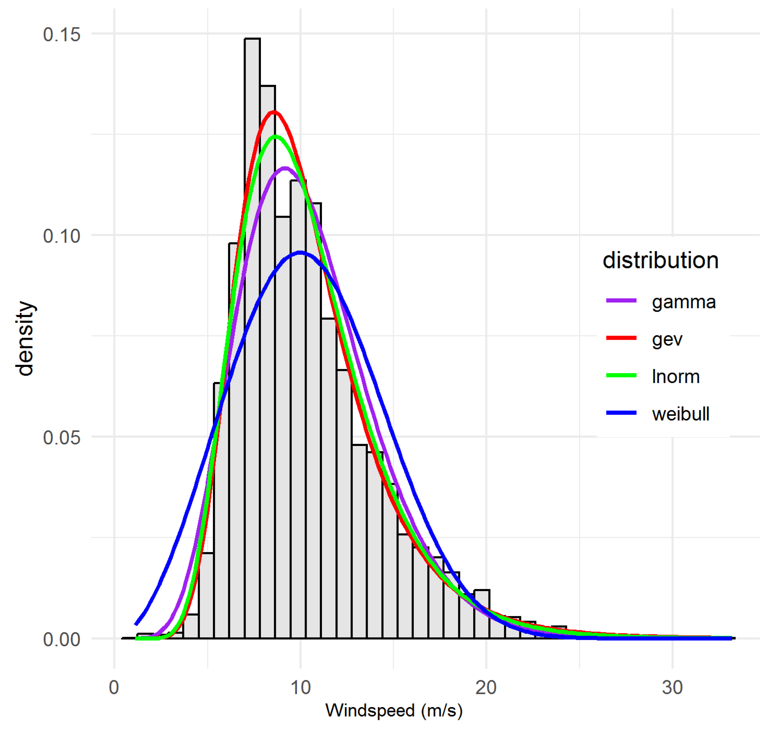
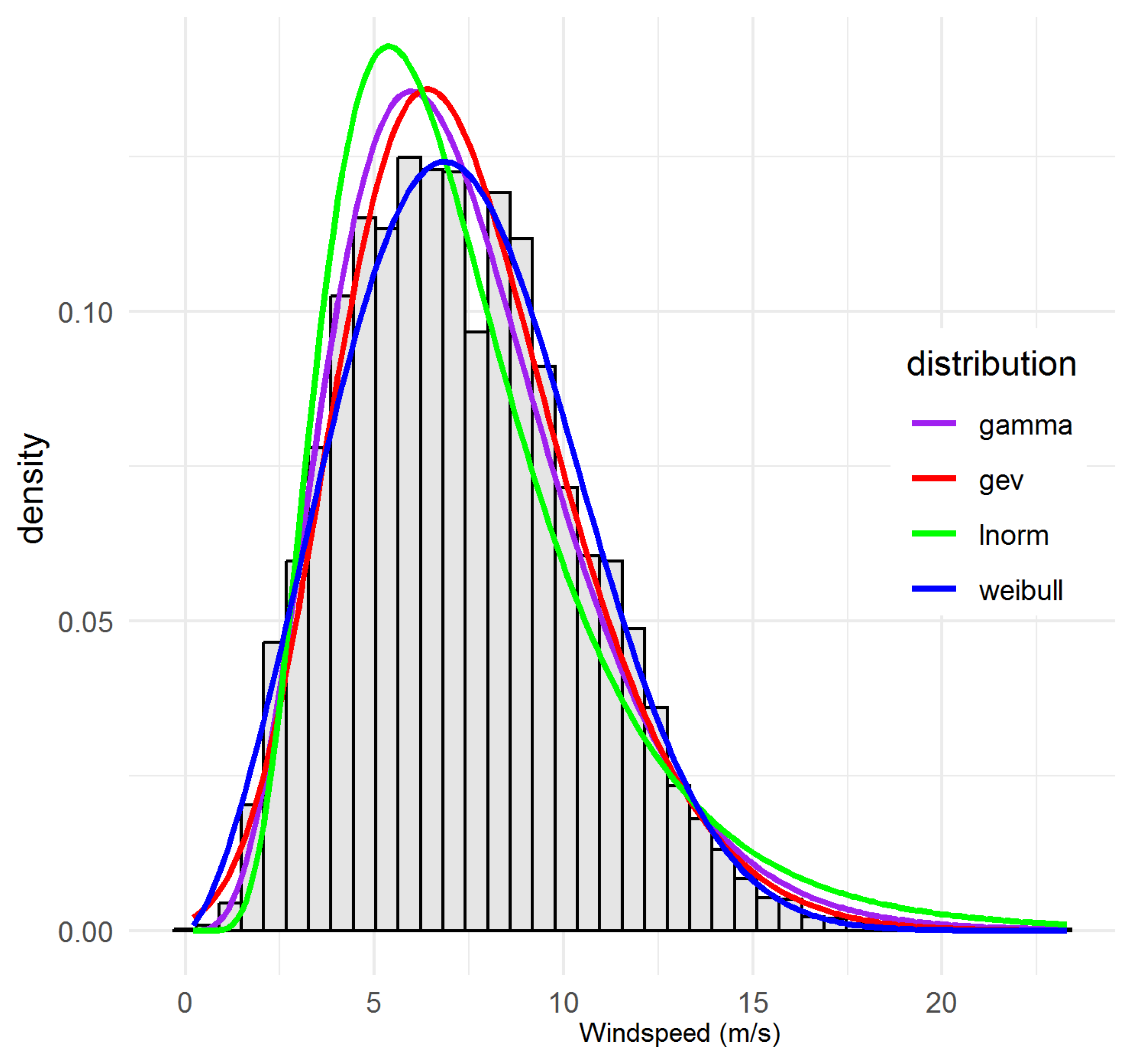
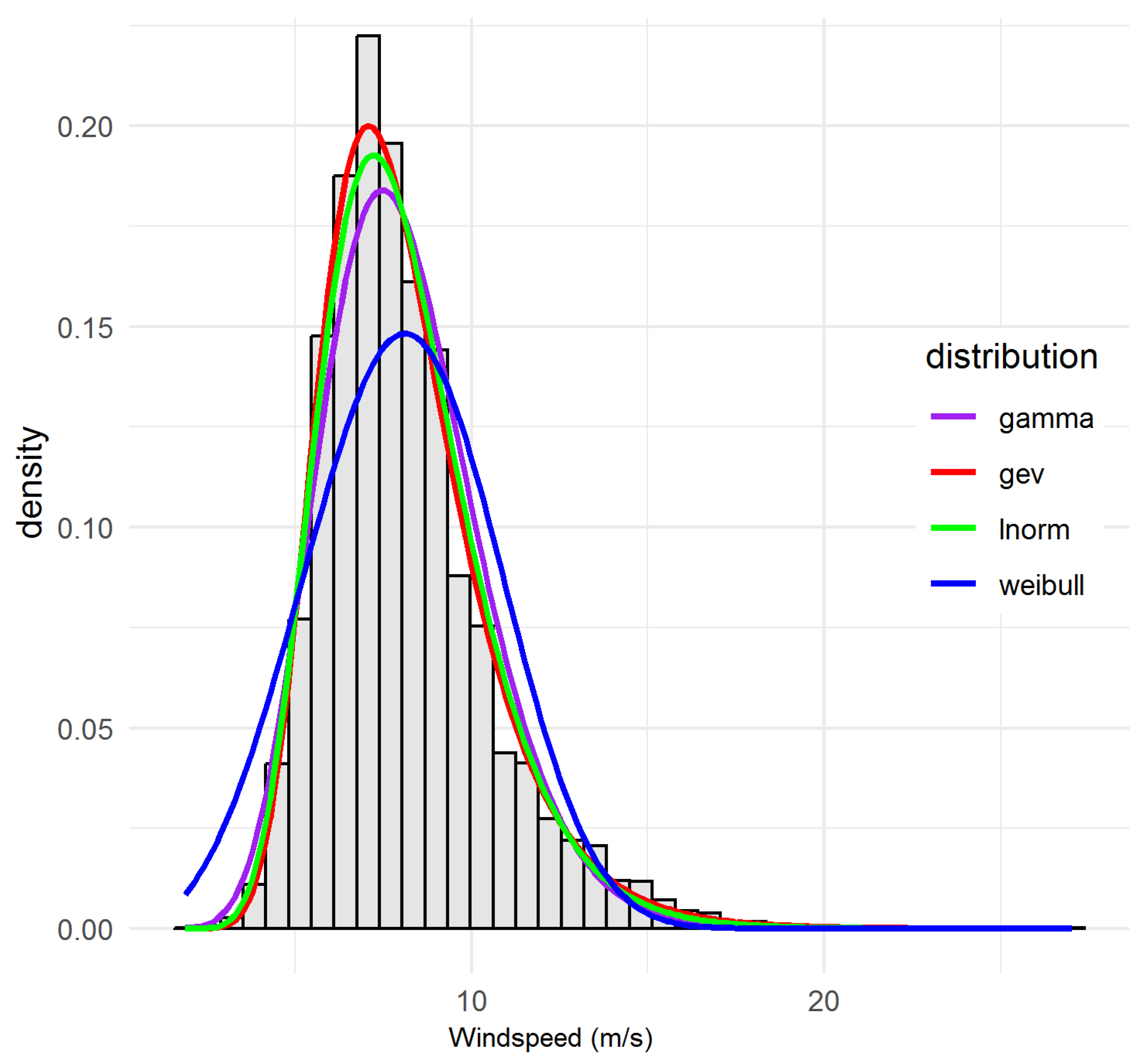
- Comprehensive Marginal Selection: Comparison of four parametric families—Weibull, Gamma, Lognormal, and GEV—fitted via maximum likelihood and, where necessary, L-moments, and evaluated through information criteria (AIC, BIC) and empirical distribution-function tests (Anderson–Darling, Cramér–von Mises, Kolmogorov–Smirnov).
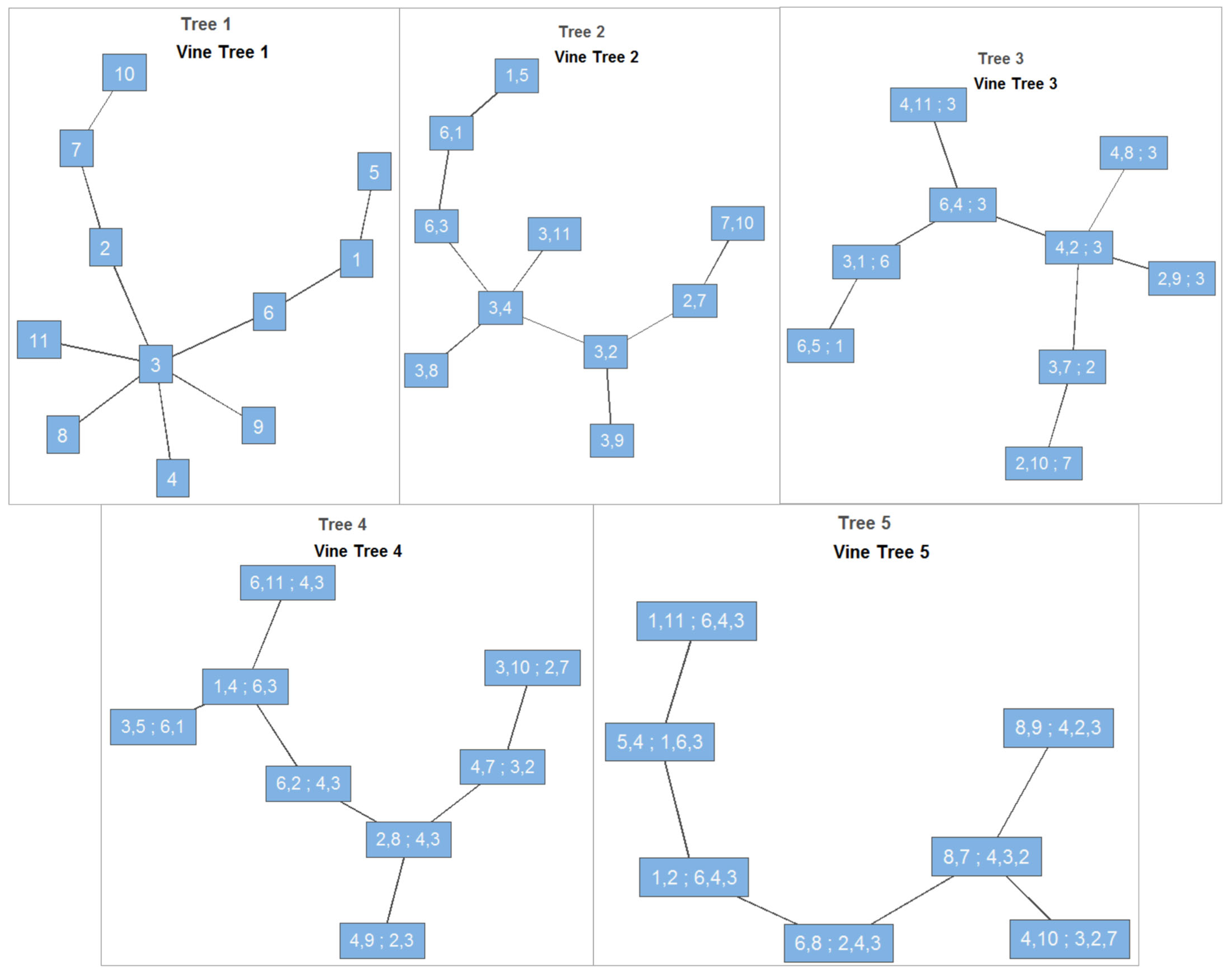
- Spatial Vine-Copula Modelling: The construction of an 11-dimensional R-vine copula tailored to the NSW–QLD network, selecting optimal bivariate copula families at each vine tree by penalised likelihood and assessing multivariate GoF via a parametric bootstrap Cramér–von Mises test.
- Engineering implications via Power-Curve Simulation based on marginal and dependence choices: Quantification of how marginal and dependence choices translate into variation in MAE and yield-uncertainty for two representative turbines (IEC V90 and E82) by generating 5000 joint synthetic windspeed series and mapping them through standard cubic-ramp power curves.
2. Literature Review
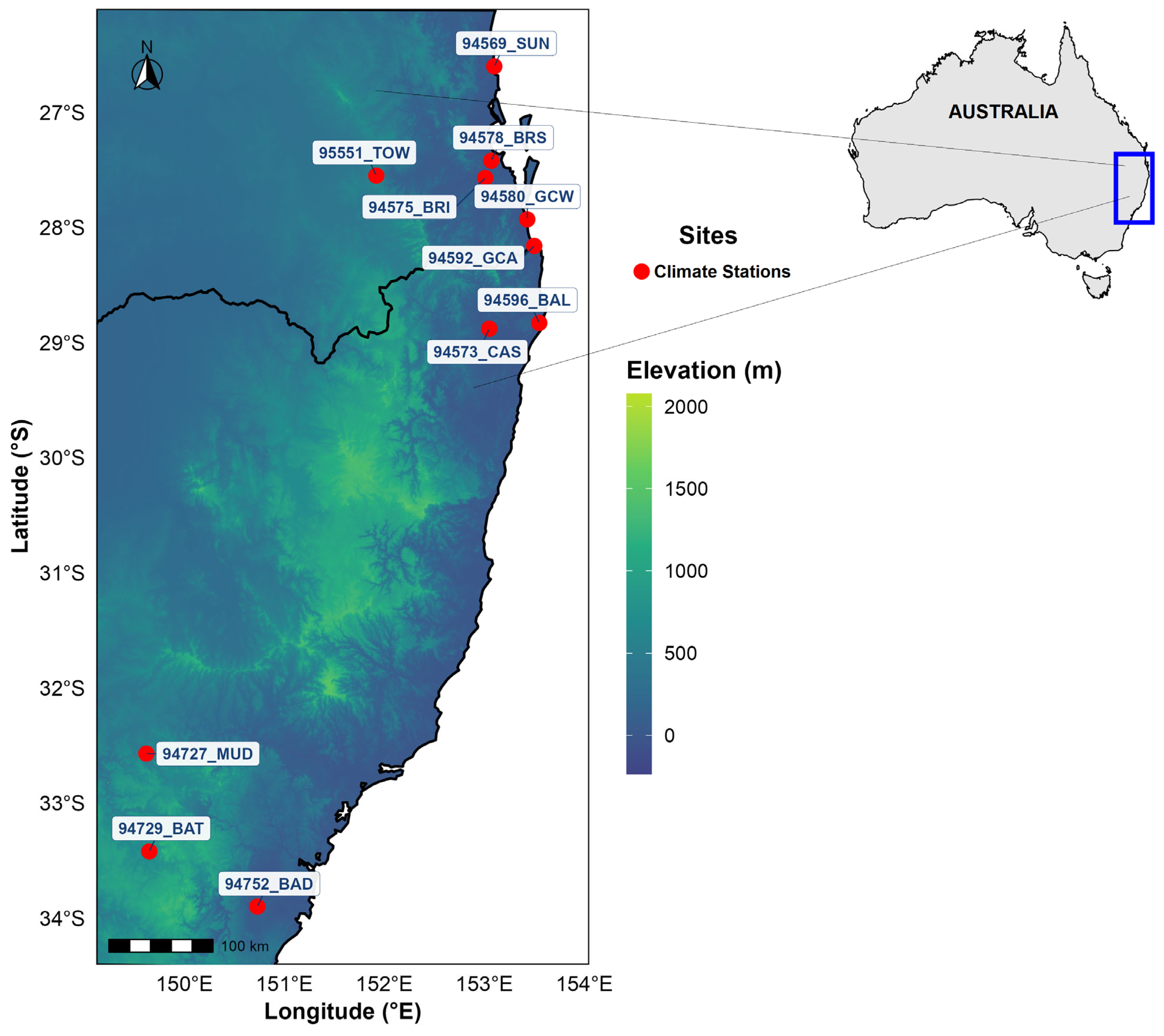
3. Study Area and Data
4. Methodology
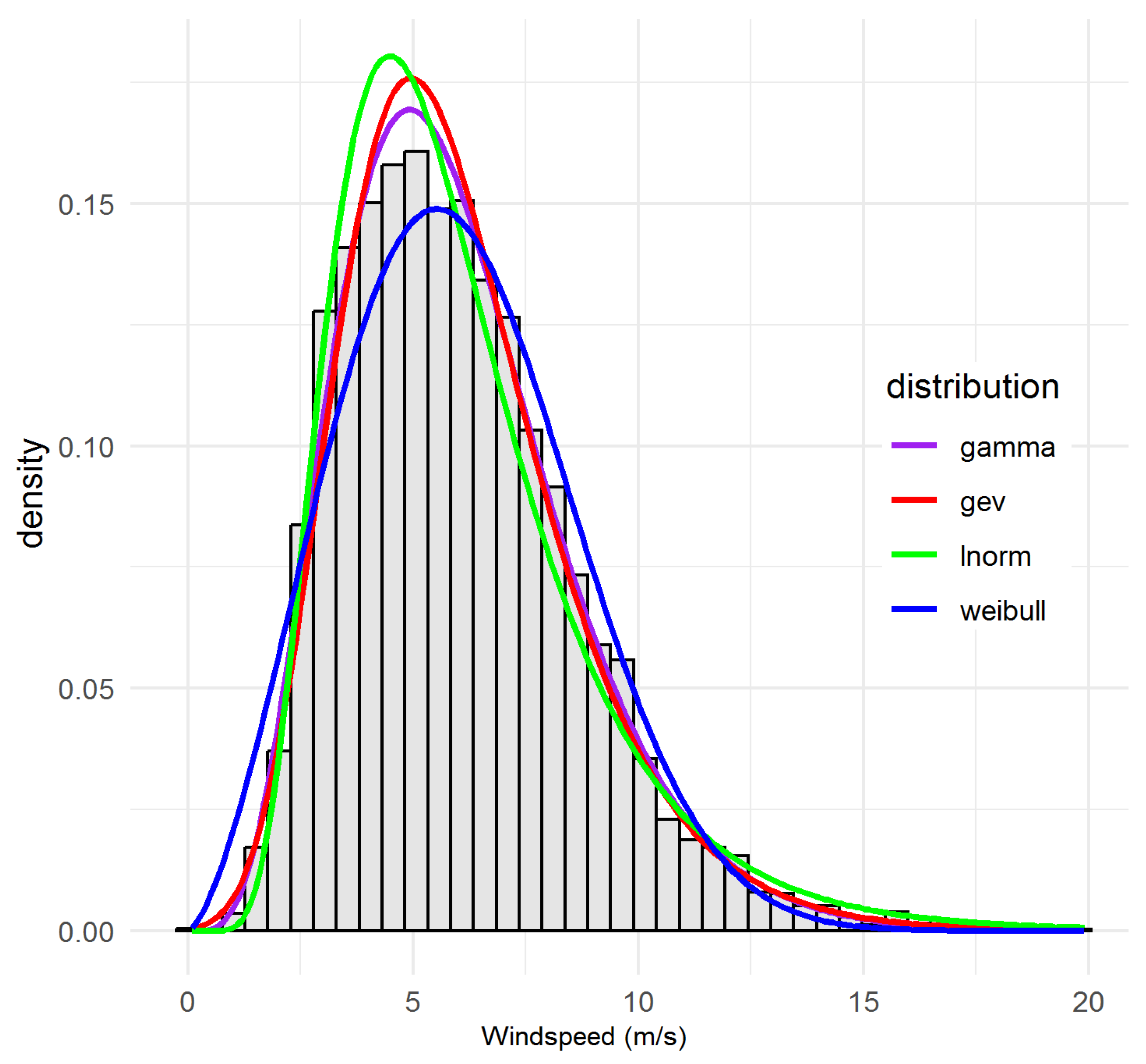
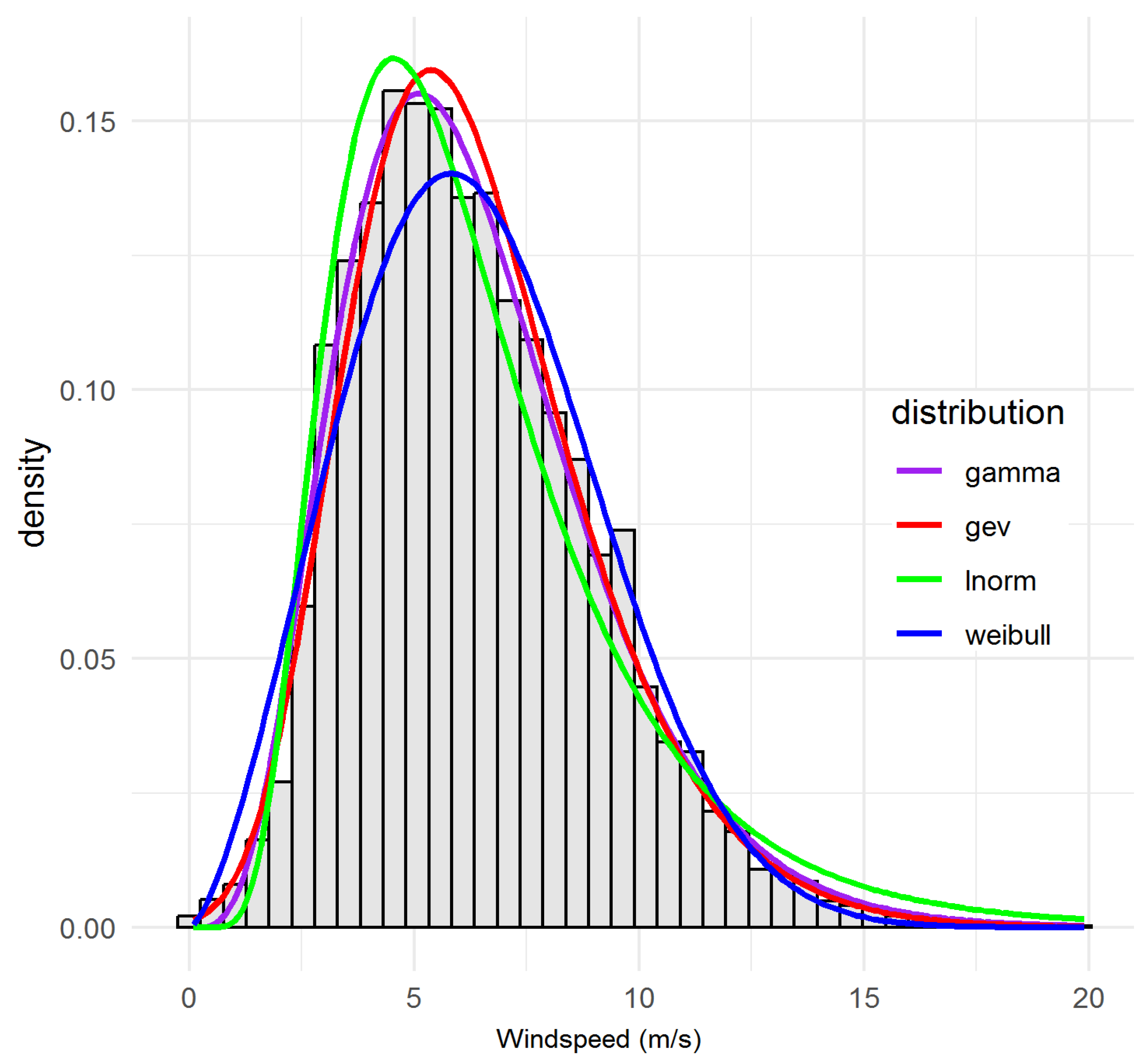
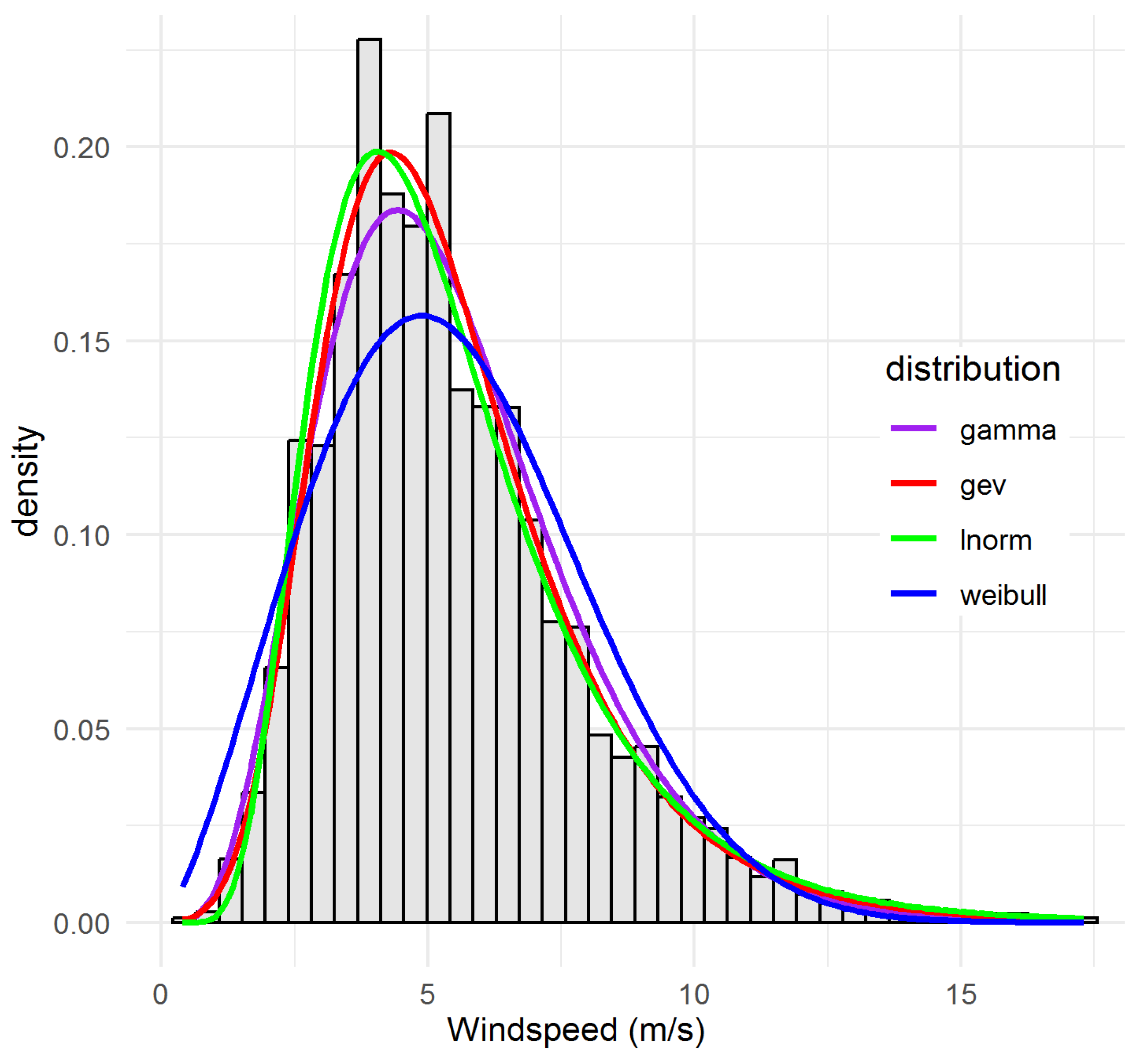
4.1. Marginal Distribution Framework and Goodness-of-Fit Metrics
- Weibull (WEI)valued for its two-parameter simplicity and closed-form mean/variance.
- Gamma (GAM)which can flexibly capture skewed shapes, especially in moderate tails.
- Lognormal (LN)often superior when low-wind probability is high.
- Generalised Extreme Value (GEV)with σ > 0 and shape ξ ∈ , to capture rare extremes.
4.1.1. Maximum Likelihood Estimation (MLE)
4.1.2. L-Moments Fallback
- Akaike Information Criterion (AIC)
- Bayesian Information Criterion (BIC)where k is the number of parameters and n the sample size.
- Anderson–Darling (AD)
- Cramér–von Mises (CvM)
- Kolmogorov–Smirnov (KS)
4.2. Vine-Copula Dependence ModellingFramework
4.2.1. Pseudo-Observations
4.2.2. R-Vine Density Factorisation
4.2.3. Pair-Copula Selection and Estimation
4.2.4. Goodness-of-Fit for the Vine Copula
- Latent Normal Test. Define by applying the univariate normal quantile element-wise. Under a correctly specified Gaussian copula, rows of Z are i.i.d. N(0, R). The Henze-Zirkler test is then applied to Z to obtain a test statistic H and p-value pHZ.
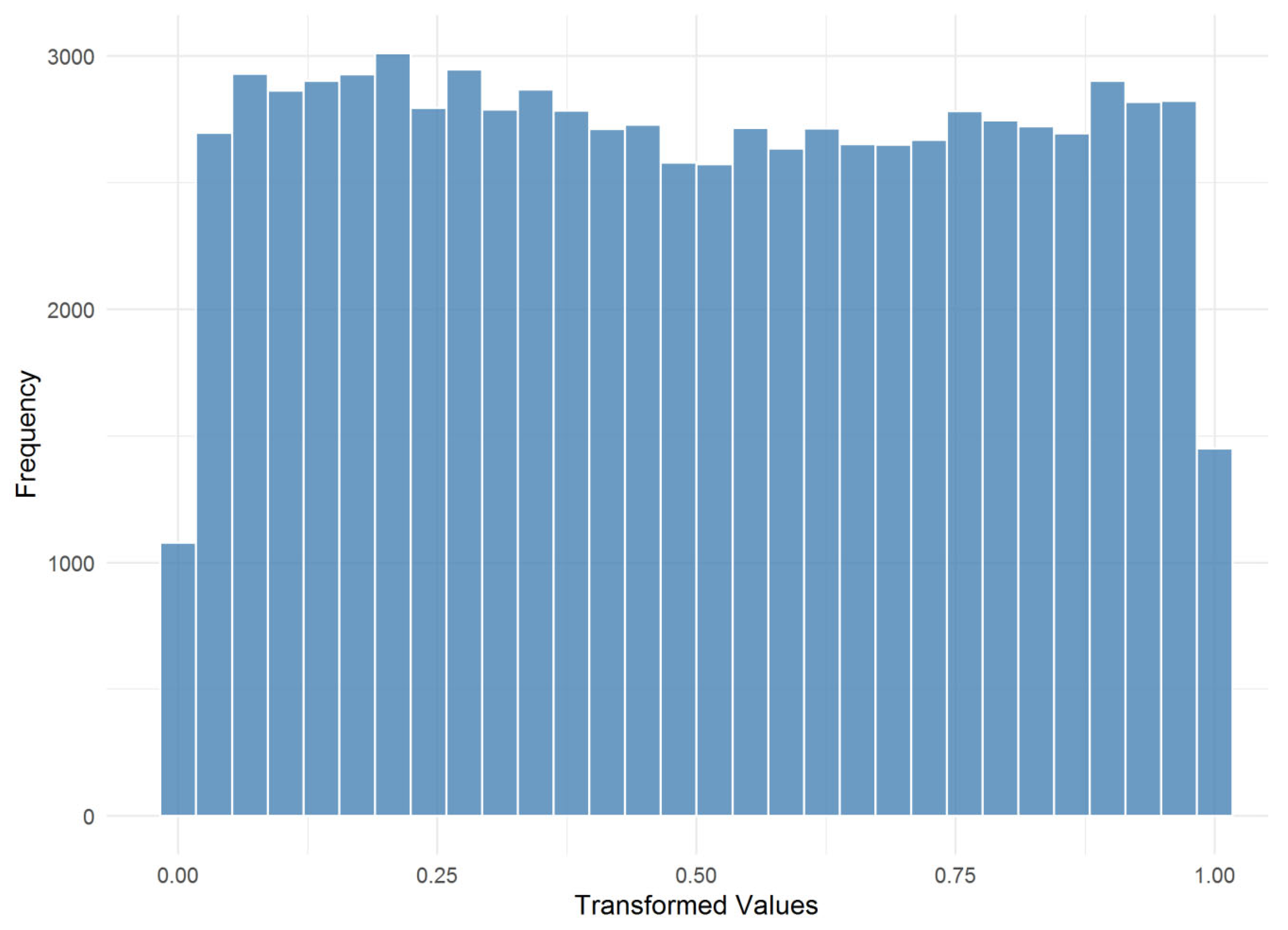
- Rosenblatt Bootstrap Test. Compute the empirical Rosenblatt transform under the fitted R-vine, flatten all entries of V into a vector v, and compute the Cramér–von Mises statistic
4.3. Composite Scoring and Distribution Ranking
- Compute the univariate GoF score as the average of the percentile ranks (across all 3 test statistics AD, CvM, KS) after reversing them so that better fits yield higher percentiles.
- Compute the copula GoF score as the percentile rank of -ln , so that smaller p-values (worse fit) correspond to lower percentiles.
- Define the composite score
4.4. Power-Curve Simulation
Windspeed Height Extrapolation
- Model Selection. For each site, pick the top two distributions d = 1, 2 by composite score.
- Joint Sampling. Simulate T = 5000 i.i.d. rows from the fitted R-vine.
- Inverse-CDF. For each site i and distribution d, obtain windspeeds
- Turbine Power. Map each simulated speed v to power via the standard cubic-ramp:where are turbine-specific constants (IECV90 and Enercon E82).
- Annual Yield Aggregation. Sum daily power over 365-day virtual years and compute the sample mean and standard deviation across the T replicates to quantify the yearly energy yield distribution for each combination of site, distribution, and turbine.
5. Results and Discussion
5.1. Marginal Fit Results—Site-by-Site Interpretation of Marginal Windspeed Parameter Estimates
5.1.1. Central Magnitude and Typical Variability
5.1.2. Shape Parameters and Spread
5.1.3. Physical Interpretation of Site Differences
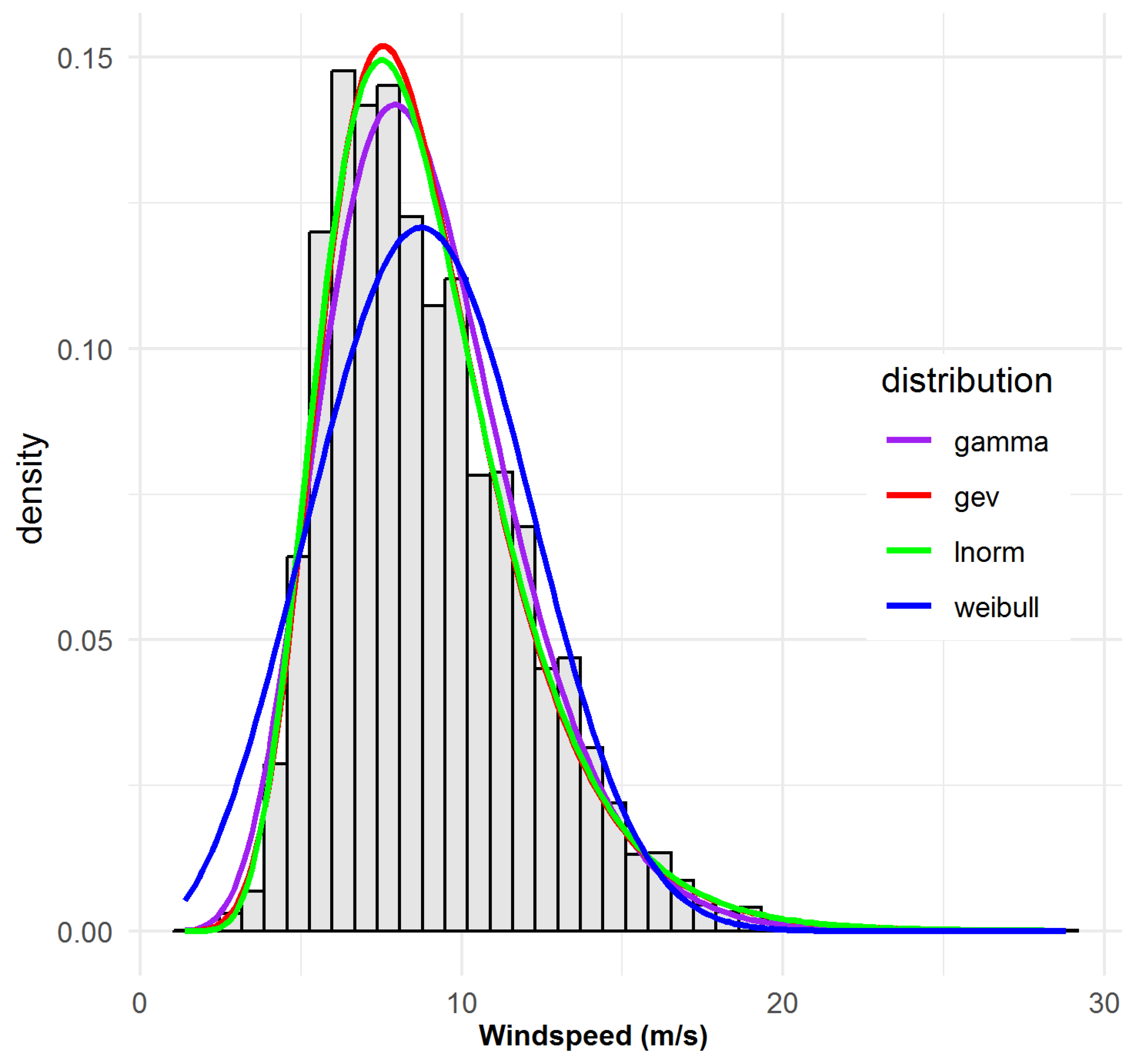
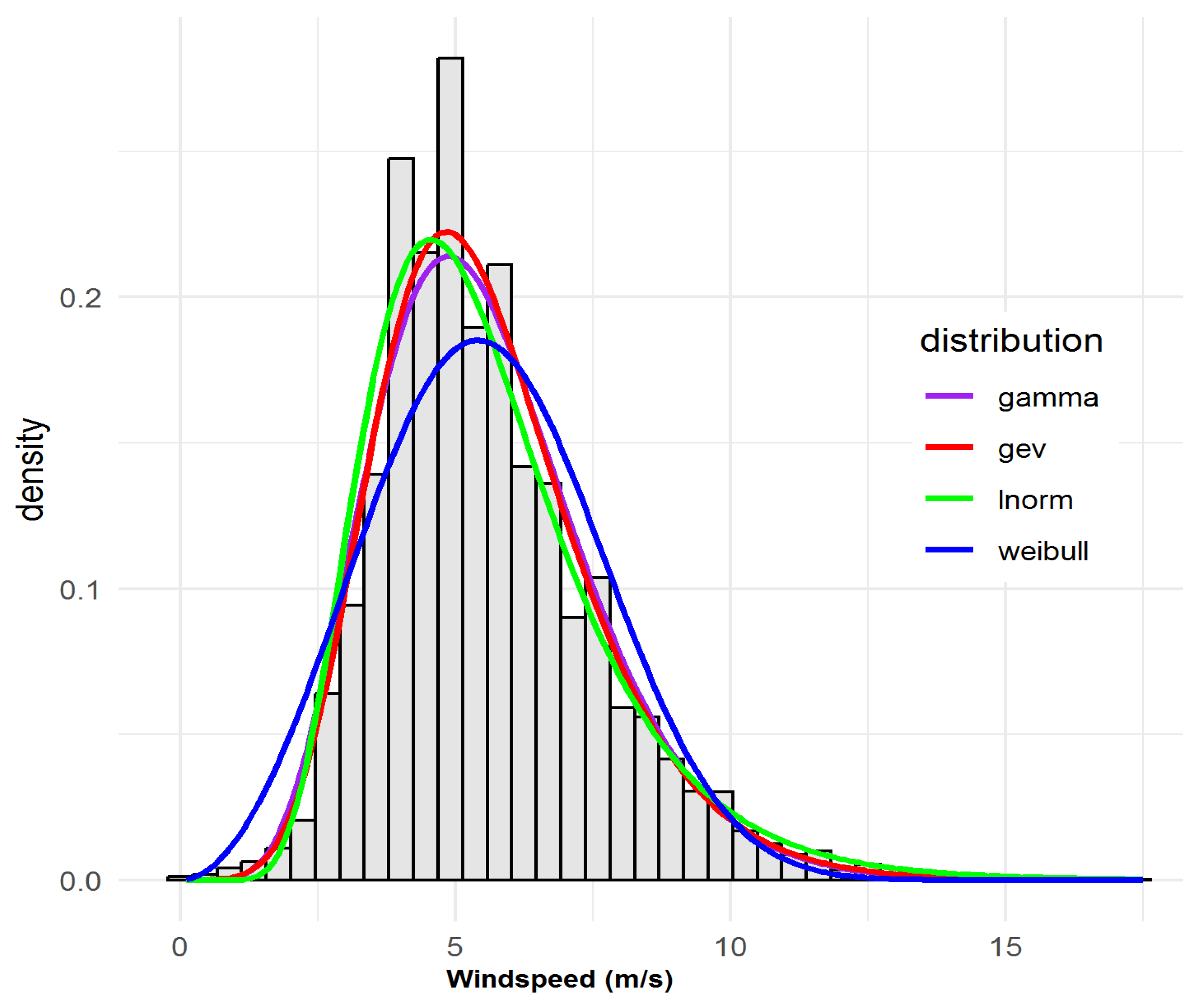
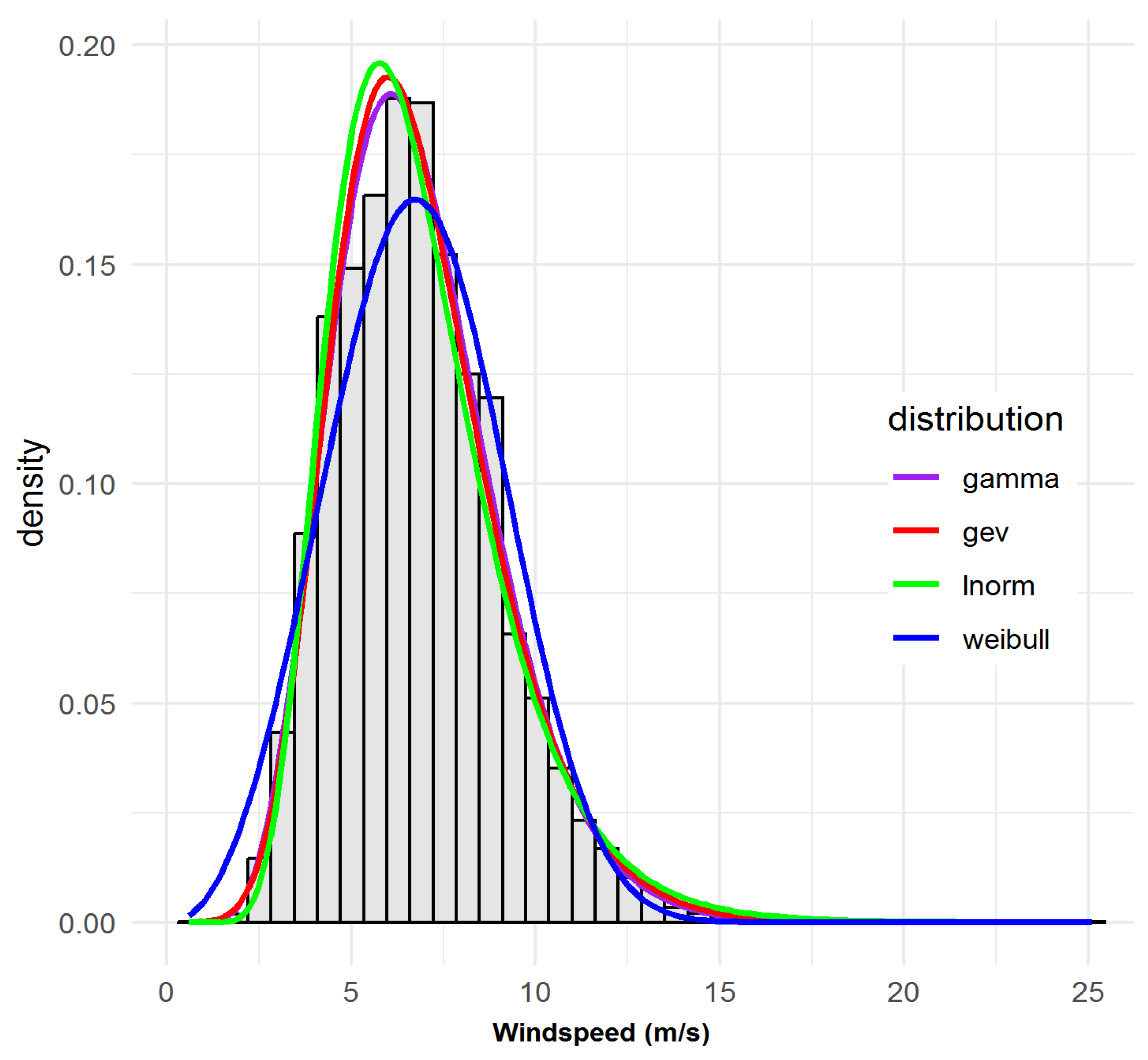
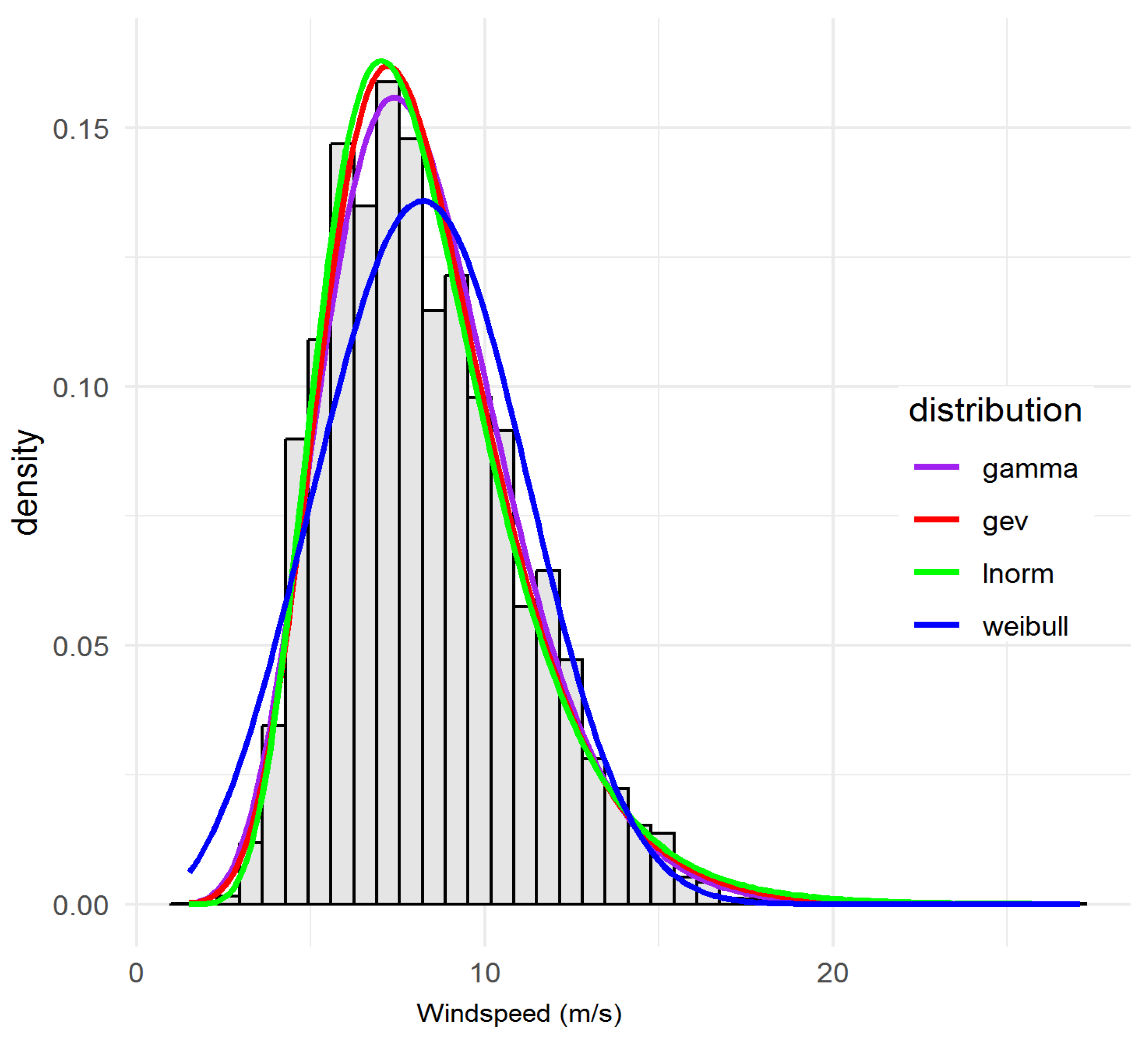
5.1.4. Summary of Univariate Fit Metrics, Goodness-of-Fit Evaluation and Site-Specific Distribution Diagnostics
5.2. Vine-Copula Dependence Modelling
5.2.1. Pseudo-Observations
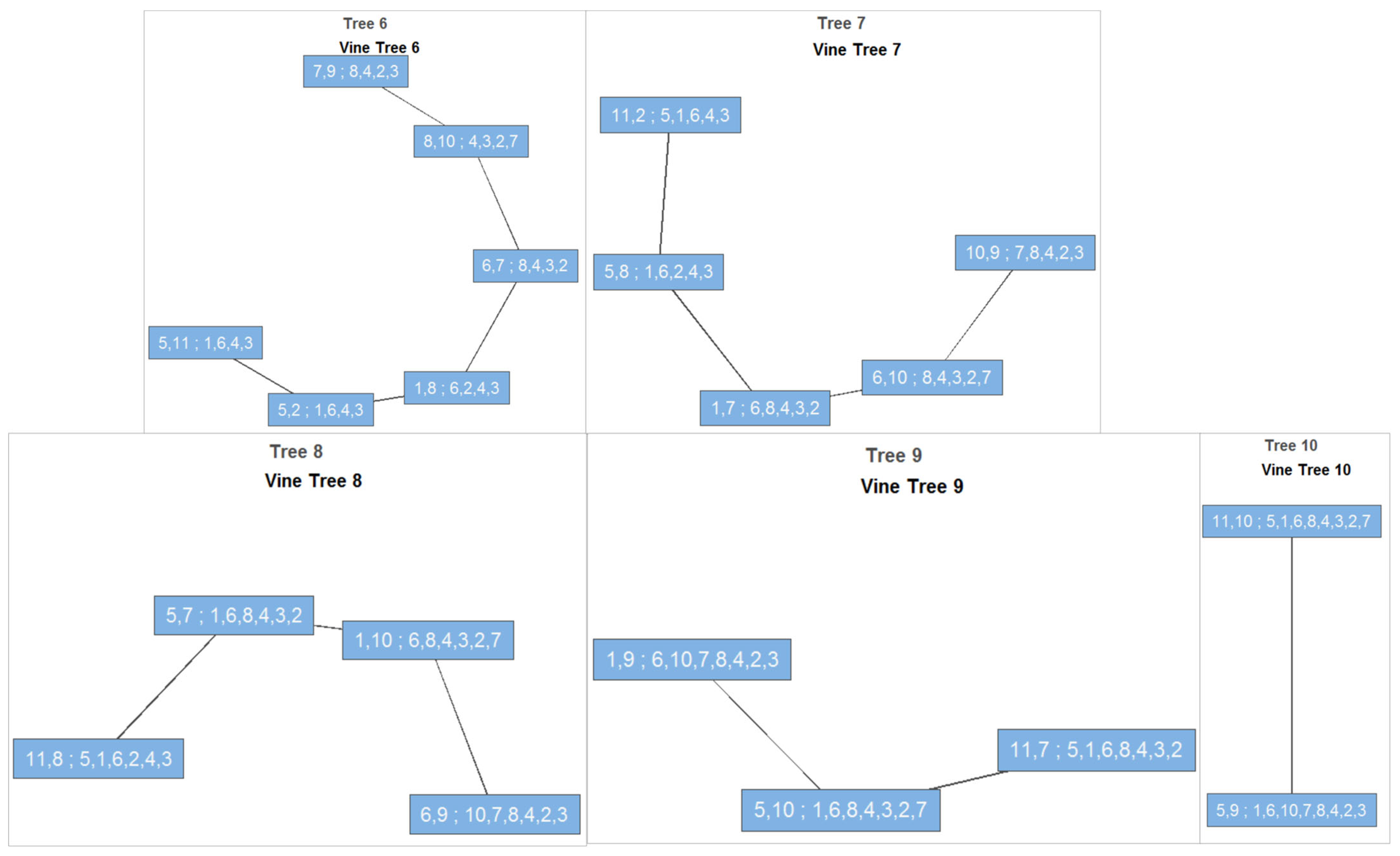
5.2.2. R-Vine Tree Structure and Pair-Copula Families
5.2.3. Goodness-of-Fit (GoF) for the Vine Copula
5.2.4. Parameter Estimates, Kendall’s τ, and Copula Selection
- Strength of Dependence: Most site pairs exhibit low to moderate positive τ, in the range 0.01–0.22. The strongest observed link τ = 0.22 between 94569_SUN and 94580_GCW directly mirrors their geographic closeness and shared exposure to onshore winds. Other moderately strong connections (τ ≈ 0.14–0.17) unite Brisbane and Gold Coast stations, confirming the existence of meteorologically coherent sub regions.
- Heterogeneity: Not all pairs are strongly connected. Negative or near-zero τ values are found for pairs with large geographic, elevational, or climatological separation (e.g., Toowoomba, Bathurst, Mudgee), consistent with locally unique wind regimes and supporting the model’s physical credibility.
- Copula Diversity: The selection of copula families is data-driven, guided by the lowest AIC values. The model is sensitive to a spectrum of behaviours: strong lower-tail dependence (Clayton), symmetric dependence (Frank/Gaussian), and independence, depending on the physical realities of each pair.
5.2.5. Frequency and Meaning of Chosen Copula Families
- Clayton dominance: Signals periods where calm conditions propagate broadly through the network, e.g., during stagnant high-pressure systems.
- Frank and Student-t: Suggest symmetric or heavy-tailed dependencies, occurring more frequently among inland pairs or at transition points between climate regimes.
- Gaussian: Selected less frequently, validating the inadequacy of normal models for these data.
- Independence: Correctly identifies weak or disconnected stations, often at geographical fringes, or across sharp orographic barriers.
5.2.6. Composite Scores: Selecting Marginal Models for Each Site
5.3. Power Curve Simulation
5.3.1. Methodological Scope and Objectives
5.3.2. Impact of Windspeed Marginal Distributions on Simulated Wind Power Yield
5.3.3. Jointly Simulated Windspeed Marginals: Physical and Statistical Insights
5.3.4. Power-Curve Convolution and Energy-Yield Distributions
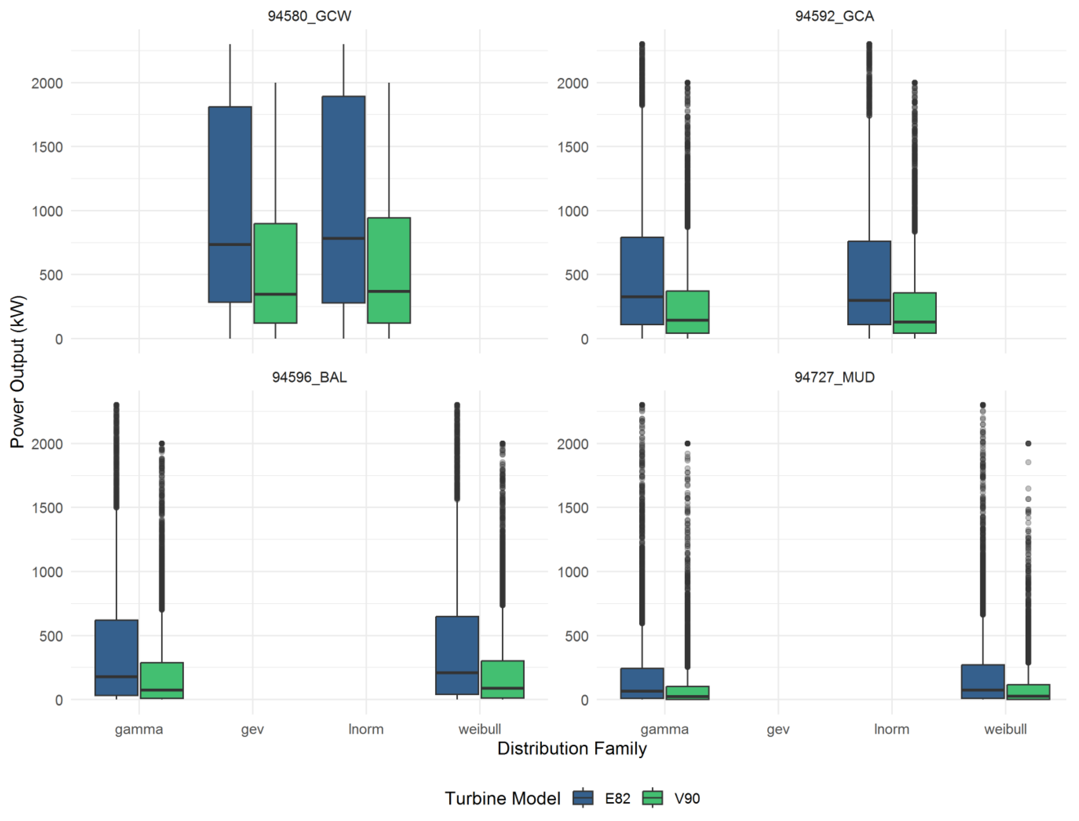
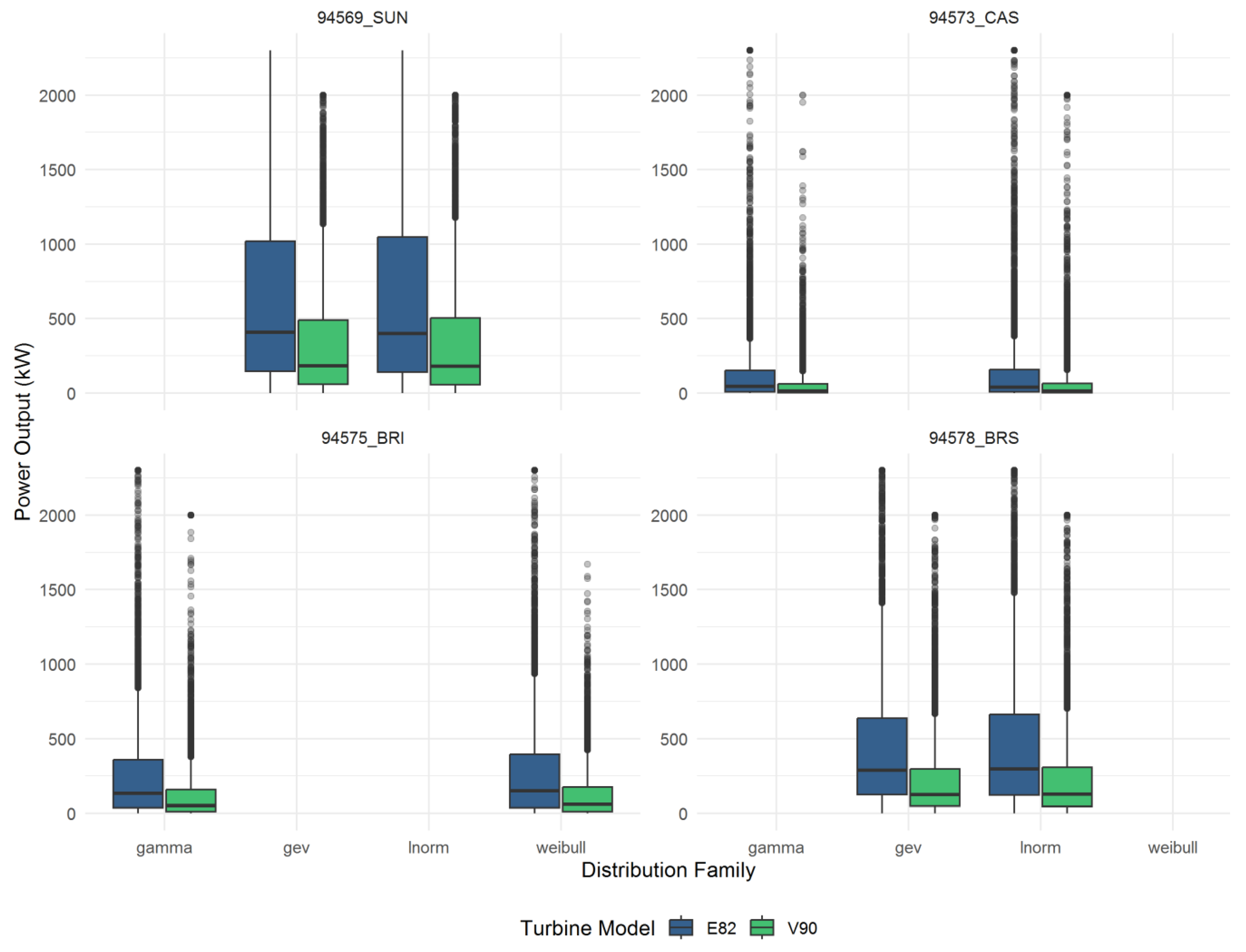
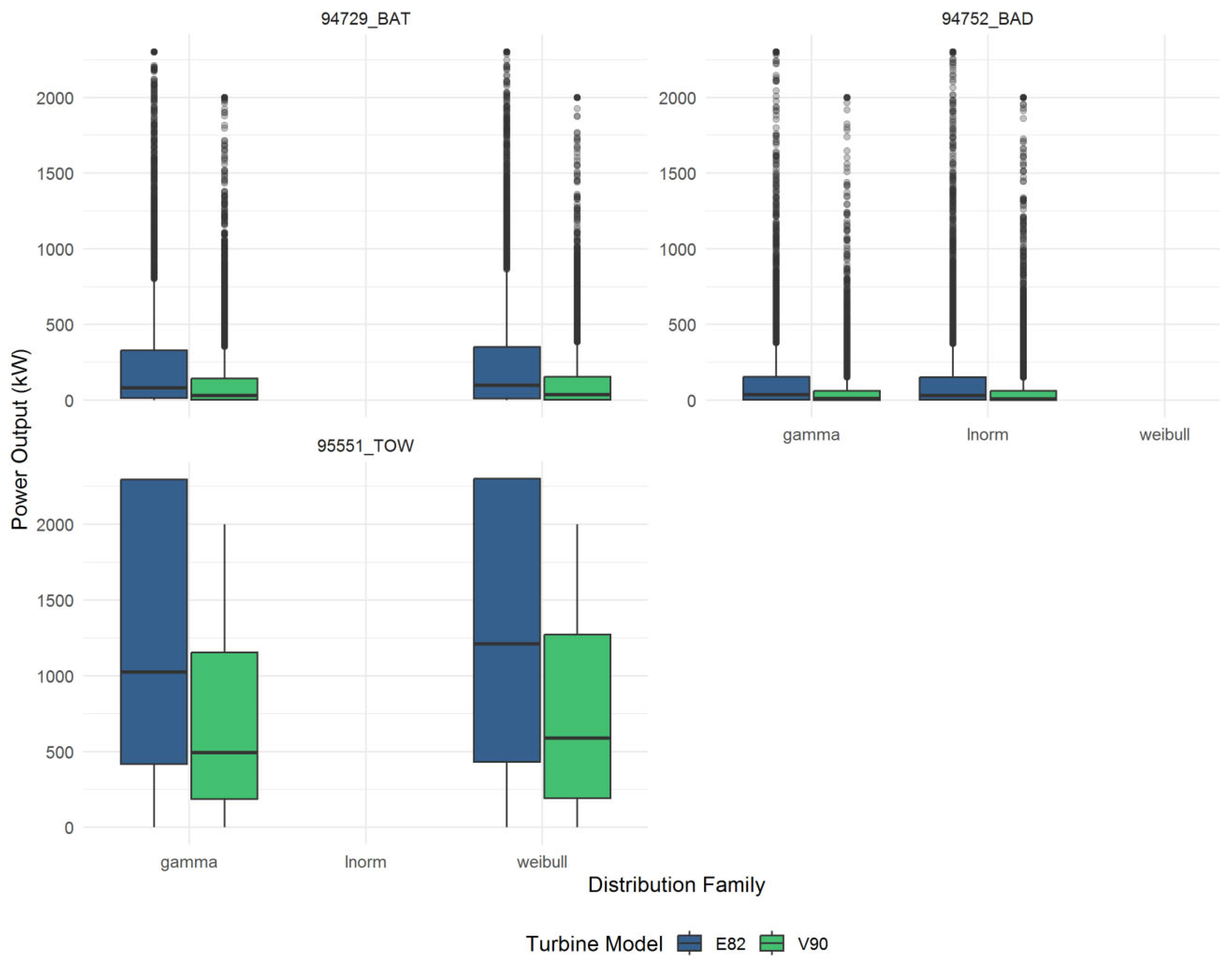
- The E82 turbine, with a lower rated windspeed and distinctive power curve, consistently achieves higher median annual yields than the V90 across all sites and marginals. This is evident in the systematically higher placement of E82 distributions in every panel.
- The breadth of the boxplots underlines substantial interannual and epistemic uncertainty, reflecting both wind climate variability and statistical fitting limitations. For high-wind sites with complex topography (e.g., Toowoomba, Gold Coast Seaway), this uncertainty range encompasses as much as 50–70% of the median value, signalling strong sensitivity to underlying wind-speed statistics.
5.3.5. Quantitative Assessment: Mean Yield and Uncertainty
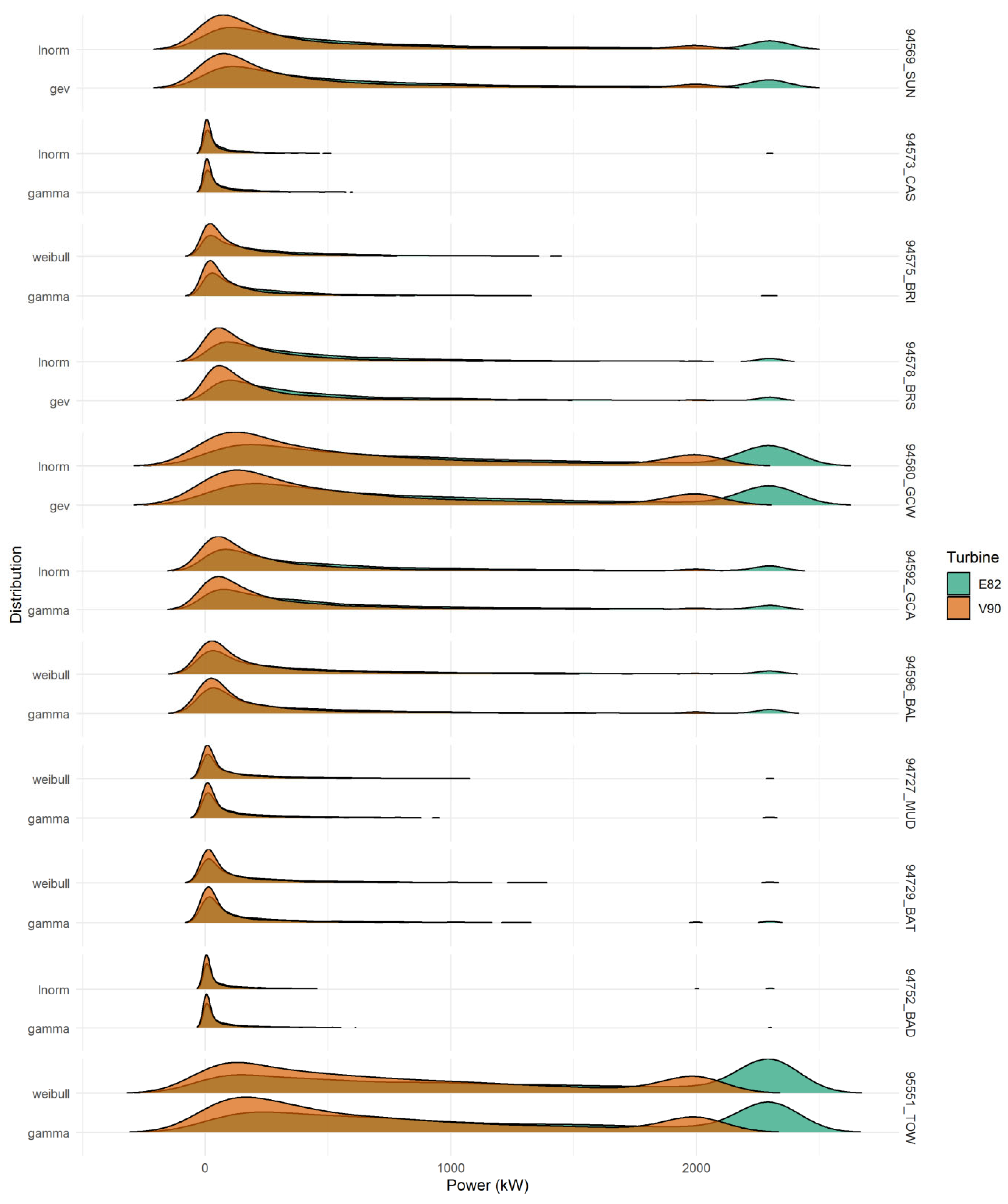
5.3.6. Annual Yield Distributions: Ridgeline Plot Insights
- Full-distribution morphology: Each horizontal “ridge” corresponds to the kernel-density estimate of 5000 annual yield simulations for a given turbine–marginal combination at each site. Sharp peaks denote tightly clustered yields; long right tails signal occasional very high-yield years.
- High wind sites (e.g., Toowoomba—95551_TOW; Gold Coast Seaway—94580_GCW): The ridges exhibit pronounced right skew and a broader basal width, reflecting both elevated mean yields and greater year-to-year variability.
- Low wind or constrained sites (e.g., Bathurst—94729_BAT; Ballina—94596_BAL): Ridges are narrow, symmetric, and sometimes truncated, indicating yields tightly bound near cut-in speeds or turbine capacity limits. The following key interpretations can be made from Figure 11:
- Skew and Tail Risk: The right-hand tail of several ridges (notably under GAM marginals) underscores the potential for rare, high-yield years—vital information for financial stress-testing and return-level analyses.
- Marginal-Driven Shifts: Across nearly all sites, GAM-based ridges shift slightly rightward and often broaden relative to LN and WEI, confirming the composite score results in Table A3: GAM tends to produce higher mean yields and larger uncertainty envelopes.
- Turbine Contrast: Enercon E82 ridges (in amber) generally dominate Vestas V90 (in teal) in both height and horizontal position reflecting the E82’s steeper power curve but exhibit greater overlap at the upper tail when using high-energy marginals, indicating similar “peak year” performance under those scenarios.
5.4. Overall Interpretation and Recommendations
- Critical Role of Marginal Selection
- 2.
- Turbine-Specific Sensitivity
6. Conclusions and Future Work
Funding
Data Availability Statement
Acknowledgments
Conflicts of Interest
Appendix A
| Site1 | Site2 | Tau | Family | θ | θ2 | AIC |
|---|---|---|---|---|---|---|
| 94569_SUN | 94573_CAS | 0.06 | 3 | 0.10 | 0 | −65.19 |
| 94569_SUN | 94575_BRI | 0.11 | 5 | 0.93 | 0 | −179.81 |
| 94569_SUN | 94578_BRS | 0.09 | 3 | 0.15 | 0 | −121.83 |
| 94569_SUN | 94580_GCW | 0.22 | 4 | 1.25 | 0 | −820.08 |
| 94569_SUN | 94592_GCA | 0.14 | 2 | 0.20 | 30 | −304.03 |
| 94569_SUN | 94596_BAL | 0.03 | 14 | 1.04 | 0 | −23.07 |
| 94569_SUN | 94727_MUD | 0.08 | 3 | 0.15 | 0 | −131.91 |
| 94569_SUN | 94729_BAT | 0.05 | 3 | 0.10 | 0 | −52.61 |
| 94569_SUN | 94752_BAD | 0.01 | 0 | 0 | 0 | 0.00 |
| 94569_SUN | 95551_TOW | 0.07 | 1 | 0.11 | 0 | −80.76 |
| 94573_CAS | 94575_BRI | 0.11 | 2 | 0.16 | 27.28 | −200.89 |
| 94573_CAS | 94578_BRS | 0.09 | 2 | 0.14 | 30 | −151.78 |
| 94573_CAS | 94580_GCW | 0.04 | 3 | 0.08 | 0 | −39.91 |
| 94573_CAS | 94592_GCA | 0.07 | 3 | 0.12 | 0 | −86.70 |
| 94573_CAS | 94596_BAL | 0.08 | 5 | 0.69 | 0 | −89.80 |
| 94573_CAS | 94727_MUD | 0.07 | 1 | 0.11 | 0 | −80.04 |
| 94573_CAS | 94729_BAT | 0.06 | 5 | 0.57 | 0 | −62.12 |
| 94573_CAS | 94752_BAD | 0.05 | 3 | 0.10 | 0 | −64.73 |
| 94573_CAS | 95551_TOW | 0.04 | 3 | 0.06 | 0 | −26.83 |
| 94575_BRI | 94578_BRS | 0.17 | 5 | 1.62 | 0 | −482.96 |
| 94575_BRI | 94580_GCW | 0.08 | 5 | 0.75 | 0 | −112.55 |
| 94575_BRI | 94592_GCA | 0.14 | 3 | 0.27 | 0 | −314.43 |
| 94575_BRI | 94596_BAL | 0.05 | 3 | 0.12 | 0 | −72.79 |
| 94575_BRI | 94727_MUD | 0.08 | 3 | 0.16 | 0 | −137.82 |
| 94575_BRI | 94729_BAT | 0.12 | 2 | 0.17 | 17.98 | −226.66 |
| 94575_BRI | 94752_BAD | 0.04 | 3 | 0.11 | 0 | −75.99 |
| 94575_BRI | 95551_TOW | 0.13 | 3 | 0.24 | 0 | −269.44 |
| 94578_BRS | 94580_GCW | 0.08 | 5 | 0.68 | 0 | −89.99 |
| 94578_BRS | 94592_GCA | 0.12 | 1 | 0.18 | 0 | −225.24 |
| 94578_BRS | 94596_BAL | 0.04 | 1 | 0.07 | 0 | −31.94 |
| 94578_BRS | 94727_MUD | 0.08 | 3 | 0.15 | 0 | −122.75 |
| 94578_BRS | 94729_BAT | 0.07 | 3 | 0.12 | 0 | −81.47 |
| 94578_BRS | 94752_BAD | 0.02 | 3 | 0.05 | 0 | −12.75 |
| 94578_BRS | 95551_TOW | 0.11 | 3 | 0.19 | 0 | −193.16 |
| 94580_GCW | 94592_GCA | 0.08 | 5 | 0.68 | 0 | −97.16 |
| 94580_GCW | 94596_BAL | 0.02 | 3 | 0.05 | 0 | −13.04 |
| 94580_GCW | 94727_MUD | 0.07 | 3 | 0.11 | 0 | −72.98 |
| 94580_GCW | 94729_BAT | 0.04 | 5 | 0.32 | 0 | −19.62 |
| 94580_GCW | 94752_BAD | −0.00 | 0 | 0 | 0 | 0.00 |
| 94580_GCW | 95551_TOW | 0.07 | 1 | 0.10 | 0 | −77.15 |
| 94592_GCA | 94596_BAL | 0.04 | 1 | 0.06 | 0 | −25.66 |
| 94592_GCA | 94727_MUD | 0.06 | 3 | 0.13 | 0 | −87.66 |
| 94592_GCA | 94729_BAT | 0.03 | 3 | 0.07 | 0 | −22.23 |
| 94592_GCA | 94752_BAD | 0.04 | 16 | 1.08 | 0 | −53.52 |
| 94592_GCA | 95551_TOW | 0.10 | 3 | 0.21 | 0 | −211.17 |
| 94596_BAL | 94727_MUD | 0.04 | 14 | 1.04 | 0 | −26.30 |
| 94596_BAL | 94729_BAT | 0.03 | 3 | 0.08 | 0 | −28.64 |
| 94596_BAL | 94752_BAD | 0.05 | 14 | 1.06 | 0 | −58.80 |
| 94596_BAL | 95551_TOW | −0.01 | 0 | 0 | 0 | 0.00 |
| 94727_MUD | 94729_BAT | 0.05 | 3 | 0.10 | 0 | −54.18 |
| 94727_MUD | 94752_BAD | 0.02 | 16 | 1.06 | 0 | −34.11 |
| 94727_MUD | 95551_TOW | 0.05 | 3 | 0.11 | 0 | −64.12 |
| 94729_BAT | 94752_BAD | 0.02 | 3 | 0.04 | 0 | −10.43 |
| 94729_BAT | 95551_TOW | 0.04 | 3 | 0.11 | 0 | −65.24 |
| 94752_BAD | 95551_TOW | 0.02 | 16 | 1.05 | 0 | −33.73 |
| Copula Family | Count |
|---|---|
| Clayton (3) | 21 |
| Frank (5) | 8 |
| Gaussian (1) | 6 |
| Student-t (2) | 4 |
| Independence(0) | 3 |
| Gumbel (4) | 1 |
| Others (14,16) | 6 |
| Site | Dist | GoF_uni | GoF_cop | Score |
|---|---|---|---|---|
| 94569_SUN | GAM | 0.067 | 0.572 | 0.218 |
| 94569_SUN | GEV | 0.033 | 0.572 | 0.195 |
| 94569_SUN | LN | 0.333 | 0.572 | 0.405 |
| 94569_SUN | WEI | 0.1 | 0.572 | 0.242 |
| 94573_CAS | GAM | 0.8 | 0.522 | 0.717 |
| 94573_CAS | GEV | 0.6 | 0.522 | 0.577 |
| 94573_CAS | LN | 0.733 | 0.522 | 0.67 |
| 94573_CAS | WEI | 0.5 | 0.522 | 0.507 |
| 94575_BRI | GAM | 0.7 | 0.793 | 0.728 |
| 94575_BRI | GEV | 0.667 | 0.793 | 0.704 |
| 94575_BRI | LN | 0.533 | 0.793 | 0.611 |
| 94575_BRI | WEI | 0.867 | 0.793 | 0.844 |
| 94578_BRS | GAM | 0.533 | 0.654 | 0.569 |
| 94578_BRS | GEV | 0.8 | 0.654 | 0.756 |
| 94578_BRS | LN | 0.767 | 0.654 | 0.733 |
| 94578_BRS | WEI | 0.3 | 0.654 | 0.406 |
| 94580_GCW | GAM | 0.233 | 0.459 | 0.301 |
| 94580_GCW | GEV | 0.333 | 0.459 | 0.371 |
| 94580_GCW | LN | 0.5 | 0.459 | 0.488 |
| 94580_GCW | WEI | 0.1 | 0.459 | 0.208 |
| 94592_GCA | GAM | 0.333 | 0.622 | 0.42 |
| 94592_GCA | GEV | 0.3 | 0.622 | 0.397 |
| 94592_GCA | LN | 0.5 | 0.622 | 0.537 |
| 94592_GCA | WEI | 0.367 | 0.622 | 0.443 |
| 94596_BAL | GAM | 0.367 | 0.256 | 0.333 |
| 94596_BAL | GEV | 0.467 | 0.256 | 0.403 |
| 94596_BAL | LN | 0.167 | 0.256 | 0.193 |
| 94596_BAL | WEI | 0.667 | 0.256 | 0.543 |
| 94727_MUD | GAM | 0.667 | 0.519 | 0.622 |
| 94727_MUD | GEV | 0.567 | 0.519 | 0.552 |
| 94727_MUD | LN | 0.433 | 0.519 | 0.459 |
| 94727_MUD | WEI | 0.767 | 0.519 | 0.692 |
| 94729_BAT | GAM | 0.733 | 0.354 | 0.619 |
| 94729_BAT | GEV | 0.7 | 0.354 | 0.596 |
| 94729_BAT | LN | 0.5 | 0.354 | 0.456 |
| 94729_BAT | WEI | 0.733 | 0.354 | 0.619 |
| 94752_BAD | GAM | 0.767 | 0.231 | 0.606 |
| 94752_BAD | GEV | 0.867 | 0.231 | 0.676 |
| 94752_BAD | LN | 0.833 | 0.231 | 0.653 |
| 94752_BAD | WEI | 0.767 | 0.231 | 0.606 |
| 95551_TOW | GAM | 0.3 | 0.507 | 0.362 |
| 95551_TOW | GEV | 0.167 | 0.507 | 0.269 |
| 95551_TOW | LN | 0.2 | 0.507 | 0.292 |
| 95551_TOW | WEI | 0.333 | 0.507 | 0.386 |
| Site | Turbine | Marginal 1 | Marginal 2 | Mean Yield M1 (kW) | Mean Yield M2 (kW) | % Diff (M1 vs. M2) | IQR M1 (kW) | IQR M2 (kW) | Comments |
|---|---|---|---|---|---|---|---|---|---|
| 94729_BAT | E82 | GAM | LN | 350 | 330 | +6% | 300 | 280 | E82 higher, moderate gamma impact |
| 94729_BAT | V90 | GAM | LN | 80 | 75 | +7% | 60 | 55 | Small difference, consistent direction |
| 94752_BAD | E82 | GAM | LN | 300 | 285 | +5% | 250 | 250 | Marginal effect similar for both curves |
| 94752_BAD | V90 | GAM | LN | 60 | 58 | +3% | 40 | 40 | Low overall yields, modest difference |
| 95551_TOW | E82 | GAM | WEI | 1100 | 1050 | +5% | 900 | 900 | Both marginals wide IQR, high wind site |
| 95551_TOW | V90 | GAM | WEI | 650 | 600 | +8% | 600 | 600 | Gamma yields notably higher |
| 94580_GCW | E82 | GAM | LN | 1200 | 1150 | +4% | 1000 | 950 | High yields, minor marginal effect |
| 94580_GCW | V90 | GAM | LN | 600 | 580 | +3% | 600 | 600 | Low-moderate difference |
| 94592_GCA | E82 | GAM | KN | 350 | 340 | +3% | 250 | 250 | Similar curves, gamma slightly higher |
| 94592_GCA | V90 | GAM | LN | 60 | 59 | +2% | 60 | 60 | Difference negligible |
| 94596_BAL | E82 | GAM | LN | 250 | 240 | +4% | 180 | 170 | Both curves wide IQR, gamma leads |
| 94596_BAL | V90 | GAM | LN | 50 | 48 | +4% | 45 | 45 | Consistent for both marginals |
| 94569_SUN | E82 | GAM | LN | 800 | 770 | +4% | 650 | 650 | High mean yield, similar spread |
| 94569_SUN | V90 | GAM | LN | 320 | 310 | +3% | 320 | 320 | Modest difference |
| 94727_MUD | E82 | GAM | LN | 460 | 430 | +7% | 350 | 350 | Gamma gives higher yield |
| 94727_MUD | V90 | GAM | LN | 110 | 100 | +10% | 130 | 120 | Larger marginal impact |
| 94573_CAS | E82 | GAM | LN | 240 | 230 | +4% | 210 | 180 | Low wind, less pronounced difference |
| 94573_CAS | V90 | GAM | LN | 60 | 58 | +4% | 70 | 70 | Small spread, small mean difference |
| 94575_BRI | E82 | GAM | LN | 290 | 270 | +7% | 250 | 230 | Slightly wider IQR for gamma |
| 94575_BRI | V90 | GAM | LN | 60 | 58 | +3% | 40 | 40 | Low difference for both turbines |
| 94578_BRS | E82 | GAM | LN | 250 | 240 | +4% | 210 | 210 | Gamma higher, IQR identical |
| 94578_BRS | V90 | GAM | LN | 60 | 59 | +2% | 70 | 70 | Across the board, E82 > V90 |
Appendix B

References
- Huang, J.; McElroy, M.B. A 32-year perspective on the origin of wind energy in a warming climate. Renew. Energy 2015, 77, 482–492. [Google Scholar] [CrossRef]
- Jung, C.; Schindler, D.; Laible, J.; Buchholz, A. Introducing a system of wind speed distributions for modeling properties of wind speed regimes around the world. Energy Convers. Manag. 2017, 144, 181–192. [Google Scholar] [CrossRef]
- Justus, C.G.; Hargraves, W.R.; Mikhail, A.; Graber, D. Methods for estimating wind speed frequency distributions. J. Appl. Meteorol. Climatol. 1978, 17, 350–353. [Google Scholar] [CrossRef]
- Bagiorgas, H.S.; Giouli, M.; Rehman, S.; Al-Hadhrami, L.M. Weibull Parameters Estimation Using Four Different Methods and Most Energy-Carrying Wind Speed Analysis. Int. J. Green Energy 2011, 8, 529–554. [Google Scholar] [CrossRef]
- Mohammadi, K.; Alavi, O.; Mostafaeipour, A.; Goudarzi, N.; Jalilvand, M. Assessing different parameters estimation methods of Weibull distribution to compute wind power density. Energy Convers. Manag. 2016, 108, 322–335. [Google Scholar] [CrossRef]
- Arslan, T.; Bulut, Y.M.; Yavuz, A.A. Comparative study of numerical methods for determining Weibull parameters for wind energy potential. Renew. Sustain. Energy Rev. 2014, 40, 820–825. [Google Scholar] [CrossRef]
- Bilir, L.; Imir, M.; Devrim, Y.; Albostan, A. Seasonal and yearly wind speed distribution and wind power density analysis based on Weibull distribution function. Int. J. Hydrogen Energy 2015, 40, 15301–15310. [Google Scholar] [CrossRef]
- Kaplan, O.; Temiz, M. A novel method based on Weibull distribution for short-term wind speed prediction. Int. J. Hydrogen Energy 2017, 42, 17793–17800. [Google Scholar] [CrossRef]
- Campos, R.; Soares, C.G. Spatial distribution of offshore wind statistics on the coast of Portugal using Regional Frequency Analysis. Renew. Energy 2018, 123, 806–816. [Google Scholar] [CrossRef]
- Hosking, J.R.M. L-moments: Analysis and estimation of distributions using linear combinations of order statistics. J. R. Stat. Soc. Ser. B Stat. Methodol. 1990, 52, 105–124. [Google Scholar] [CrossRef]
- Teyabeen, A.A.; Akkari, F.R.; Jwaid, A.E. Comparison of seven numerical methods for estimating Weibull parameters for wind energy applications. In Proceedings of the 2017 UKSim-AMSS 19th International Conference on Computer Modelling & Simulation (UKSim), Cambridge, UK, 5–7 April 2017; pp. 173–178. [Google Scholar]
- Nelsen, R.B. An Introduction to Copulas; Springer: New York, NY, USA, 2006. [Google Scholar]
- Tastu, J.; Pinson, P.; Madsen, H. Space-time trajectories of wind power generation: Parametrized precision matrices under a Gaussian copula approach. In Modeling and Stochastic Learning for Forecasting in High Dimensions; Springer International Publishing: Cham, Germany, 2015; pp. 267–296. [Google Scholar]
- Malvaldi, A.; Weiss, S.; Infield, D.; Browell, J.; Leahy, P.; Foley, A.M. A spatial and temporal correlation analysis of aggregate wind power in an ideally interconnected Europe. Wind. Energy 2017, 20, 1315–1329. [Google Scholar] [CrossRef]
- Wang, Z.; Wang, W.; Liu, C.; Wang, B. Forecasted scenarios of regional wind farms based on regular vine copulas. J. Mod. Power Syst. Clean Energy 2019, 8, 77–85. [Google Scholar] [CrossRef]
- Aas, K.; Czado, C.; Frigessi, A.; Bakken, H. Pair-copula constructions of multiple dependence. Insur. Math. Econ. 2009, 44, 182–198. [Google Scholar] [CrossRef]
- Dissmann, J.; Brechmann, E.C.; Czado, C.; Kurowicka, D. Selecting and estimating regular vine copulae and application to financial returns. Comput. Stat. Data Anal. 2013, 59, 52–69. [Google Scholar] [CrossRef]
- Masseran, N. Integrated approach for the determination of an accurate wind-speed distribution model. Energy Convers. Manag. 2018, 173, 56–64. [Google Scholar] [CrossRef]
- Chowdhury, S.; Zhang, J.; Messac, A.; Castillo, L. Optimizing the arrangement and the selection of turbines for wind farms subject to varying wind conditions. Renew. Energy 2013, 52, 273–282. [Google Scholar] [CrossRef]
- Katsigiannis, Y.A.; Stavrakakis, G.S. Estimation of wind energy production in various sites in Australia for different wind turbine classes: A comparative technical and economic assessment. Renew. Energy 2014, 67, 230–236. [Google Scholar] [CrossRef]
- Ouarda Taha, B.M.J.; Charron, C. On the mixture of wind speed distribution in a Nordic region. Energy Convers. Manag. 2018, 174, 33–44. [Google Scholar] [CrossRef]
- Ouarda Taha, B.M.J.; Charron, C. Non-stationary statistical modelling of wind speed: A case study in eastern Canada. Energy Convers. Manag. 2021, 236, 114028. [Google Scholar] [CrossRef]
- Houndekindo, F.; Ouarda Taha, B.M.J. A non-parametric approach for wind speed distribution mapping. Energy Convers. Manag. 2023, 296, 117672. [Google Scholar] [CrossRef]
- Houndekindo, F.; Ouarda Taha, B.M.J. Prediction of hourly wind speed time series at unsampled locations using machine learning. Energy 2024, 299, 131518. [Google Scholar] [CrossRef]
- Lu, X.; McElroy, M.B. Global potential for wind-generated electricity. In Wind Energy Engineering; Academic Press: London, UK, 2023; pp. 47–61. [Google Scholar]
- Wang, C.-H.; Holmes, J.D. Exceedance rate, exceedance probability, and the duality of GEV and GPD for extreme hazard analysis. Nat. Hazards 2020, 102, 1305–1321. [Google Scholar] [CrossRef]
- Rocha, P.A.C.; de Sousa, R.C.; de Andrade, C.F.; da Silva, M.E.V. Comparison of seven numerical methods for determining Weibull parameters for wind energy generation in the northeast region of Brazil. Appl. Energy 2012, 89, 395–400. [Google Scholar] [CrossRef]
- Fawad, M.; Yan, T.; Chen, L.; Huang, K.; Singh, V.P. Multiparameter probability distributions for at-site frequency analysis of annual maximum wind speed with L-Moments for parameter estimation. Energy 2019, 181, 724–737. [Google Scholar] [CrossRef]
- Wang, W.; Gao, Y.; Ikegaya, N. Approximating wind speed probability distributions around a building by mixture weibull distribution with the methods of moments and L-moments. J. Wind. Eng. Ind. Aerodyn. 2025, 257, 106001. [Google Scholar] [CrossRef]
- Molina-Aguilar, J.P.; Gutierrez-Lopez, A.; Raynal-Villaseñor, J.A.; Garcia-Valenzuela, L.G. Optimization of Parameters in the Generalized Extreme-Value Distribution Type 1 for Three Populations Using Harmonic Search. Atmosphere 2019, 10, 257. [Google Scholar] [CrossRef]
- Stephens, M.A. EDF statistics for goodness of fit and some comparisons. J. Am. Stat. Assoc. 1974, 69, 730–737. [Google Scholar] [CrossRef]
- Razali, N.M.; Wah, Y.B. Power comparisons of shapiro-wilk, kolmogorov-smirnov, lilliefors and anderson-darling tests. J. Stat. Model. Anal. 2011, 2, 21–33. [Google Scholar]
- Evans, D.L.; Drew, J.H.; Leemis, L.M. The distribution of the Kolmogorov–Smirnov, Cramer–von Mises, and Anderson–Darling test statistics for exponential populations with estimated parameters. In Computational Probability Applications; Springer International Publishing: Cham, Germany, 2016; pp. 165–190. [Google Scholar]
- Chau, T.T.; Nguyen, T.T.H.; Nguyen, L.; Do, T.D. Wind Speed Probability Distribution Based on Adaptive Bandwidth Kernel Density Estimation Model for Wind Farm Application. Wind. Energy 2025, 28, e2970. [Google Scholar] [CrossRef]
- Chen, X.; Han, J.; Zheng, T.; Zhang, P.; Duan, S.; Miao, S. A Vine-Copula Based Voltage State Assessment with Wind Power Integration. Energies 2019, 12, 2019. [Google Scholar] [CrossRef]
- Veeramachaneni, K.; Cuesta-Infante, A.; O’Reilly, U.M. Copula graphical models for wind resource estimation. In Proceedings of the 24th International Conference on Artificial Intelligence, Buenos Aires, Argentina, 25–31 July 2015; pp. 2646–2654. [Google Scholar]
- Yoo, J.; Son, Y.; Yoon, M.; Choi, S. A Wind Power Scenario Generation Method Based on Copula Functions and Forecast Errors. Sustainability 2023, 15, 16536. [Google Scholar] [CrossRef]
- Shahirinia, A.; Farahmandfar, Z.; Bina, M.T.; Henderson, S.B.; Ashtary, M. Spatial modeling sensitivity analysis: Copula selection for wind speed dependence. AIP Adv. 2024, 14, 045047. [Google Scholar] [CrossRef]
- Peng, X.; Li, Y. Forecasting Wind Power Scenarios of Multiple Wind Farms Based on Vine Spatiotemporal Copula. Available online: https://ssrn.com/abstract=4206878 (accessed on 3 September 2025).
- Cai, J.; Xu, Q.; Cao, M.; Yang, Y. Capacity Credit Evaluation of Correlated Wind Resources Using Vine Copula and Improved Importance Sampling. Appl. Sci. 2019, 9, 199. [Google Scholar] [CrossRef]
- Karakaş, A.M. Using copulas for modeling dependence in wind power. Asian J. Eng. Technol. 2019, 7, 33–49. [Google Scholar] [CrossRef]
- Goh, H.H.; Peng, G.; Zhang, D.; Dai, W.; Kurniawan, T.A.; Goh, K.C.; Cham, C.L. A New Wind Speed Scenario Generation Method Based on Principal Component and R-Vine Copula Theories. Energies 2022, 15, 2698. [Google Scholar] [CrossRef]
- Wang, Z.; Wang, W.; Liu, C.; Wang, Z.; Hou, Y. Probabilistic Forecast for Multiple Wind Farms Based on Regular Vine Copulas. IEEE Trans. Power Syst. 2017, 33, 578–589. [Google Scholar] [CrossRef]
- Huang, Y.; Zhang, Z.; Li, X.; Xie, J.; Lee, K.Y. Layered-Vine Copula-Based Wind Speed Prediction Using Spatial Correlation and Meteorological Influence. IEEE Trans. Instrum. Meas. 2023, 72, 1–12. [Google Scholar] [CrossRef]
- Vincent, C.L.; Dowdy, A.J. Multi-scale variability of southeastern Australian wind resources. Atmospheric Meas. Tech. 2024, 24, 10209–10223. [Google Scholar] [CrossRef]
- Gu, H.; Mao, Y. Multi-Timescale Characteristics of Southwestern Australia Nearshore Surface Current and Its Response to ENSO Revealed by High-Frequency Radar. Remote. Sens. 2024, 16, 209. [Google Scholar] [CrossRef]
- AS/NZS 3580.14:2014; Methods for Sampling and Analysis of Ambient Air—Part 14: Meteorological Monitoring for Ambient Air Quality Monitoring Applications. Standards Australia: Sydney, Australia; Standards New Zealand: Wellington, New Zealand, 2014.
- Stull, R.B. Mean boundary layer characteristics. In An Introduction to Boundary Layer Meteorology; Springer: Dordrecht, The Netherlands, 1988; pp. 1–27. [Google Scholar]
- Hosking, J.R.M.; Wallis, J.R. Regional Frequency Analysis; Cambridge University Press: Cambridge, UK, 1997; p. 240. [Google Scholar]
| Parameter | Specification | Standard |
|---|---|---|
| Measurement Height | 10 m | AS/NZS 3580.14:2014, WMO |
| Averaging Period | 10 min | International meteorological standard |
| Instrument Type | Cup anemometer | WMO threshold ≤ 0.5 m/s |
| Quality Control | Automated QC procedures | BOM protocols |
| Data Standards | WMO compliance | AS/NZS 3580.14:2014 |
| Site Name | SiteID | Lat | Lon | Elev (m) | Mean (m/s) | St Dev (m/s) | Stdev/Mean (%) | Min | Max | n (obs) | Skew |
|---|---|---|---|---|---|---|---|---|---|---|---|
| Sunshine Coast | 94569_SUN | −26.6 | 153.1 | 4 | 8.89 | 3.03 | 34.1% | 1.4 | 28.8 | 7289 | 0.84 |
| Casino Airport | 94573_CAS | −28.88 | 153.05 | 22 | 5.57 | 1.97 | 35.4% | 0.1 | 17.5 | 7289 | 0.89 |
| Brisbane Archerfield Airport | 94575_BRI | −27.57 | 153.01 | 19.2 | 6.79 | 2.21 | 32.5% | 0.6 | 25.1 | 7289 | 0.7 |
| Brisbane Airport | 94578_BRS | −27.42 | 153.07 | 6 | 8.1 | 2.35 | 29.0% | 1.9 | 27 | 7289 | 1.16 |
| Gold Coast Seaway | 94580_GCW | −27.93 | 153.43 | 3 | 10.39 | 3.8 | 36.6% | 1.1 | 33.2 | 7289 | 1.19 |
| Gold Coast Airport | 94592_GCA | −28.16 | 153.5 | 6.4 | 8.26 | 2.71 | 32.8% | 1.5 | 27.1 | 7289 | 0.67 |
| Ballina Gateway | 94596_BAL | −28.83 | 153.55 | 2 | 7.36 | 3.08 | 41.8% | 0.2 | 23.3 | 7289 | 0.5 |
| Mudgee Airport | 94727_MUD | −32.57 | 149.62 | 472 | 6.01 | 2.55 | 42.4% | 0.1 | 19.9 | 7289 | 0.81 |
| Bathurst Airport | 94729_BAT | −33.42 | 149.65 | 745 | 6.35 | 2.71 | 42.7% | 0.1 | 19.9 | 7289 | 0.7 |
| Badgerys Creek Airport | 94752_BAD | −33.9 | 150.73 | 82 | 5.46 | 2.44 | 44.7% | 0.4 | 17.3 | 7289 | 1.14 |
| Toowoomba Airport | 95551_TOW | −27.55 | 151.92 | 642 | 10.86 | 3.39 | 31.2% | 2.9 | 29.7 | 7289 | 0.53 |
| Site | WEI (k) | WEI (c) | GAM (α) | GAM (β) | LN (μ) | LN (σ) | GEV (μ) | GEV (σ) | GEV (ξ) |
|---|---|---|---|---|---|---|---|---|---|
| 94569_SUN | 3.07/3.23 | 9.94/9.92 | 9.08/8.72 | 0.98/1.02 | 2.13/2.13 | 0.34/0.33 | 7.52/7.52 | 2.42/2.46 | −0.01/0.02 |
| 94573_CAS | 2.94/3.09 | 6.23/6.23 | 7.99/8.27 | 0.70/1.48 | 1.65/1.66 | 0.37/0.34 | 4.72/4.69 | 1.66/1.59 | −0.07/0.03 |
| 94575_BRI | 3.21/3.39 | 7.57/7.56 | 9.43/9.45 | 0.72/1.39 | 1.86/1.87 | 0.33/0.32 | 2.96/5.87 | 2.30/1.95 | −0.04/0.11 |
| 94578_BRS | 3.45/3.86 | 8.97/8.96 | 13.09/12.91 | 0.62/1.60 | 2.05/2.05 | 0.28/0.28 | 7.06/7.04 | 1.84/1.78 | −0.01/−0.02 |
| 94580_GCW | 2.82/2.98 | 11.66/11.64 | 8.31/7.96 | 1.25/0.77 | 2.28/2.28 | 0.35/0.35 | 8.65/8.61 | 2.82/2.78 | 0.04/−0.06 |
| 94592_GCA | 3.22/3.37 | 9.21/9.20 | 9.51/9.21 | 0.87/1.11 | 2.06/2.06 | 0.33/0.32 | 7.06/7.07 | 2.27/2.33 | −0.06/0.08 |
| 94596_BAL | 2.57/2.57 | 8.30/8.29 | 5.27/5.50 | 1.40/0.72 | 1.90/1.92 | 0.47/0.40 | 6.06/6.09 | 2.73/2.79 | −0.11/0.14 |
| 94727_MUD | 2.50/2.52 | 6.78/6.77 | 5.53/5.52 | 1.09/0.92 | 1.70/1.71 | 0.45/0.41 | 4.87/4.89 | 2.09/2.14 | −0.04/0.05 |
| 94729_BAT | 2.48/2.51 | 7.16/7.16 | 5.11/5.41 | 1.24/0.85 | 1.75/1.77 | 0.48/0.41 | 5.18/5.18 | 2.31/2.32 | −0.08/0.08 |
| 94752_BAD | 2.36/2.38 | 6.17/6.16 | 5.34/5.22 | 0.96/1.05 | 1.60/1.61 | 0.45/0.43 | 4.34/4.34 | 1.85/1.85 | 0.02/−0.03 |
| 95551_TOW | 3.41/3.55 | 12.08/12.06 | 10.21/10.04 | 1.06/0.92 | 2.34/2.34 | 0.32/0.31 | 9.41/9.43 | 2.98/3.05 | −0.10/0.12 |
| Site | Best-Fit Distribution | AD | CvM | KS | AIC | BIC | Runner-Up (AIC) |
|---|---|---|---|---|---|---|---|
| 94569_SUN | LN | 119.33 | 17.37 | 0.030 | 37,551 | 37,565 | GEV |
| 94573_CAS | LN | 61.93 | 8.34 | 0.048 | 31,779 | 31,793 | GAM |
| 94575_BRI | WEI | 76.70 | 10.60 | 0.048 | 33,933 | 33,947 | LN |
| 94578_BRS | GEV | 67.81 | 8.99 | 0.030 | 33,437 | 33,458 | LN |
| 94580_GCW | LN | 102.87 | 14.65 | 0.036 | 40,401 | 40,415 | GEV |
| 94592_GCA | LN | 114.26 | 16.21 | 0.029 | 36,293 | 36,307 | GAM |
| 94596_BAL | WEI | 89.86 | 12.47 | 0.021 | 38,158 | 38,172 | GEV |
| 94727_MUD | WEI | 85.99 | 12.17 | 0.038 | 35,468 | 35,482 | LN |
| 94729_BAT | GAM | 87.38 | 12.37 | 0.020 | 36,520 | 36,534 | GEV |
| 94752_BAD | LN | 71.71 | 9.58 | 0.029 | 33,586 | 33,600 | GAM |
| 95551_TOW | WEI | 116.60 | 17.24 | 0.050 | 40,477 | 40,491 | LN |
| Statistic | Value |
|---|---|
| Henze–Zirkler H | 0.000143 |
| p-value | 0.99994 |
Disclaimer/Publisher’s Note: The statements, opinions and data contained in all publications are solely those of the individual author(s) and contributor(s) and not of MDPI and/or the editor(s). MDPI and/or the editor(s) disclaim responsibility for any injury to people or property resulting from any ideas, methods, instructions or products referred to in the content. |
© 2025 by the author. Licensee MDPI, Basel, Switzerland. This article is an open access article distributed under the terms and conditions of the Creative Commons Attribution (CC BY) license (https://creativecommons.org/licenses/by/4.0/).
Share and Cite
Haddad, K. An Integrated Goodness-of-Fit and Vine Copula Framework for Windspeed Distribution Selection and Turbine Power-Curve Assessment in New South Wales and Southern East Queensland. Atmosphere 2025, 16, 1068. https://doi.org/10.3390/atmos16091068
Haddad K. An Integrated Goodness-of-Fit and Vine Copula Framework for Windspeed Distribution Selection and Turbine Power-Curve Assessment in New South Wales and Southern East Queensland. Atmosphere. 2025; 16(9):1068. https://doi.org/10.3390/atmos16091068
Chicago/Turabian StyleHaddad, Khaled. 2025. "An Integrated Goodness-of-Fit and Vine Copula Framework for Windspeed Distribution Selection and Turbine Power-Curve Assessment in New South Wales and Southern East Queensland" Atmosphere 16, no. 9: 1068. https://doi.org/10.3390/atmos16091068
APA StyleHaddad, K. (2025). An Integrated Goodness-of-Fit and Vine Copula Framework for Windspeed Distribution Selection and Turbine Power-Curve Assessment in New South Wales and Southern East Queensland. Atmosphere, 16(9), 1068. https://doi.org/10.3390/atmos16091068


