Article

Evaluation of Correction Methods for ERA5 Shortwave Radiation Biases in China’s Second-Step Topographic Region: A Case Study of Hubei Province

1
Southwest Electric Power Design Institute Co., Ltd. of China Power Engineering Consulting Group, Chengdu 610021, China
2
Hubei Meteorological Service Center, Wuhan 430205, China
*
Author to whom correspondence should be addressed.
Atmosphere 2025, 16(9), 1008; https://doi.org/10.3390/atmos16091008
Submission received: 10 June 2025 / Revised: 16 July 2025 / Accepted: 18 July 2025 / Published: 26 August 2025

Abstract

This study evaluates three bias correction methods, Ridge Regression, Random Forest, and FM-CNN-LSTM, to enhance ERA5 shortwave radiation estimates over Hubei Province, located within China’s second-step topographic region. Observations from six photovoltaic stations revealed significant systematic biases in the original ERA5 dataset, particularly overestimations (~50–100 W/m2) of peak radiation and underestimations during cloudy periods. Random Forest consistently provided the best corrections, achieving the highest correlation coefficients (0.84–0.88), lowest RMSE (86.14 W/m2 at Wuhan station), and smallest MAE (60.05 W/m2 at Wuhan station). Ridge Regression delivered stable but slightly inferior improvements, while FM-CNN-LSTM showed notable inconsistencies. Spatially, Random Forest-corrected data exhibited realistic radiation patterns aligned with complex topography, highlighting northeastern and eastern Hubei (>1350 kWh/m2 annually) as ideal regions for photovoltaic development. Overall, the Random Forest method is recommended as the optimal bias correction approach, substantially improving solar radiation estimates critical for renewable energy planning in complex terrains.

1. Introduction

Solar energy has emerged as a critical renewable energy resource due to its sustainability and potential to significantly reduce greenhouse gas emissions. Accurate estimation of solar radiation, particularly shortwave radiation, is crucial for photovoltaic (PV) power generation, energy grid management, and climate studies. Precise solar irradiance forecasts enable more efficient balancing of power supply and demand, facilitating energy storage management and energy market participation, thus enhancing overall grid stability and economic planning [1,2,3,4]. Any bias in solar radiation data can considerably affect solar energy forecasts, potentially leading to inefficiencies and increased operational costs [5,6].
Reanalysis datasets, especially the European Centre for Medium-Range Weather Forecasts (ECMWF) ERA5 dataset [7], are widely used in solar radiation studies due to their global coverage and high spatiotemporal resolution. ERA5 has shown significant improvement over its predecessor ERA-Interim, offering enhanced accuracy in estimating surface solar radiation at various temporal scales [7,8]. However, despite these improvements, biases persist due to inherent uncertainties in cloud representation, aerosol interactions, and complex terrain influences, particularly noticeable over regions such as China [8,9,10]. Validation studies have shown that ERA5 can overestimate hourly global horizontal irradiance, highlighting the need for effective bias correction methodologies [11].
Bias correction methods for solar radiation data range from traditional statistical adjustments, such as Ridge Regression (RR), to advanced machine learning techniques, including Random Forest and deep learning models [1,3,4,12,13]. Simple regression models have traditionally been employed due to their ease of implementation and interpretability. These methods effectively reduce systematic biases but may inadequately capture nonlinear patterns and complex interactions inherent in solar radiation data [12,14].
Advanced machine learning algorithms, notably Random Forest, have been increasingly applied in environmental data correction due to their ability to model nonlinear relationships and interactions between multiple variables. RF has demonstrated superior performance in correcting biases in environmental datasets such as snow water equivalent, precipitation, and solar radiation [5,9,12]. Studies employing RF for bias correction have shown significant improvements in the accuracy of corrected datasets over linear regression, especially when nonlinear interactions between predictors and outcomes are prevalent [12].
Recently, deep learning approaches, particularly hybrid models combining convolutional neural networks (CNN) and long short-term memory (LSTM) units, have gained popularity due to their capacity for capturing complex spatial–temporal dependencies in data [5,9,15]. Models such as FMCNN-LSTM integrate convolutional layers, which effectively capture localized spatial patterns, and LSTM units, proficient in modeling temporal dependencies. These hybrid models have shown promising results in correcting biases in numerical weather prediction outputs, significantly outperforming simpler methods in various environmental applications, including solar radiation forecasts [9]. Specifically, hybrid deep learning models have been shown to substantially reduce errors in bias-corrected solar radiation predictions by accounting for both spatial and temporal complexities that simpler models often miss [5].
The goal of this study is to evaluate the correction performance of three methods, Ridge Regression, Random Forest, and FMCNN-LSTM, on ERA5-derived solar shortwave radiation data. Observational solar radiation data from several photovoltaic (PV) stations across Hubei Province, China, representing diverse land cover types (forests, grasslands, and agricultural lands), serve as the benchmark for evaluating these correction methods. Hubei Province is strategically chosen due to its varied topography and complex terrain, characteristic of China’s second geomorphological step (Figure 1), making it representative of regions with challenging solar resource estimation conditions [15]. Complex terrains influence solar radiation significantly by inducing localized shading and cloud formations, exacerbating biases in reanalysis data [11]. Therefore, evaluating correction methods across diverse surface types in Hubei ensures the robustness of the methodology and its generalizability to other complex terrain regions.
By comprehensively comparing these methods, this study aims to identify the most effective technique for correcting biases in ERA5 solar radiation data over the second topographic step of China, thereby enhancing the reliability of solar resource assessments and forecasts. Improving the accuracy of solar radiation estimates through effective bias correction is essential for optimizing renewable energy integration into power grids and supporting sustainable energy development. The remainder of the manuscript is organized as follows: Section 2 describes the data and methods utilized in this study. Section 3 presents the evaluation and comparative analysis of the correction results. Conclusions and discussions are provided in Section 4.

2. Data and Methods

2.1. Data

The hourly observational radiation data used to evaluate the correction results were collected from six photovoltaic (PV) stations distributed across Hubei Province, China. Among these stations, Wuhan (WH) and Yichang (YC) are national-level stations, while Xiaogan (XG), Jingzhou (JZ), Suizhou (SZ), and Nanzhang (NZ) operate as provincial-level observatories. The geographic locations of these stations are illustrated in Figure 1. Each station exhibits unique topographical and environmental characteristics (Table 1). For example, Wuhan, the capital city of Hubei Province, is situated on the eastern Jianghan Plain, featuring abundant water resources and relatively flat terrain. Conversely, the NZ station, located in the mountainous and hilly region of northwestern Hubei Province, represents significantly different topographical conditions. Additionally, the selected stations cover diverse land cover types, including forests, cultivated lands, and paddy fields, with detailed descriptions provided in Table 1. Considering the integrated effects of terrain, topography, and climatic conditions, the six stations are classified into three distinct categories: mountainous and forested regions (NZ and YC), cultivated mountainous areas (SZ), and plain regions characterized by paddy fields (JZ, XG, and WH). These classifications capture typical variations in elevation and land cover encountered within China’s second-step topographic region.
ERA5 is the fifth-generation atmospheric reanalysis dataset produced by the European Centre for Medium-Range Weather Forecasts (ECMWF) [7]. It provides global atmospheric variables at high temporal and spatial resolutions, covering the period from 1950 to the present. Specifically, the ERA5 dataset includes downward shortwave radiation flux at the Earth’s surface, integrating the effects of clouds, aerosols, and atmospheric gases. These radiation data are available hourly, with a horizontal spatial resolution of approximately 27 km.
In this study, for each ground station, we selected the nearest ERA5 grid point to the station location for data pairing, since the grid centers may not exactly coincide with station coordinates. The spatial distance between the station and the matched ERA5 grid center is typically within 5–17 km. No temporal shift was applied, as both ERA5 and observational records are hourly and aligned by timestamp. Moreover, ERA5 and observational radiation data from January to November 2022 (8016 h) are utilized to develop the correction models, whereas data from December 2022 (744 h) are employed to independently validate these models. The rationale for this data selection is as follows: (1) 2022 was chosen due to the high quality and completeness of observational data in Hubei, with over 98% data coverage across all stations; (2) using January to November for training ensures full seasonal coverage, allowing the models to learn from a wide range of meteorological conditions; and (3) December was withheld as a validation period because it is characterized by low solar angles and frequent cloud cover, which pose challenges for solar radiation modeling and thus offer a stringent test for model performance.

2.2. Methods

2.2.1. Correction Models

This study employs three distinct correction models: Ridge Regression, Random Forest, and Factorization Machine-Convolutional Neural Network-Long Short-Term Memory (FM-CNN-LSTM). Each model was selected based on its capability to address specific biases present in reanalysis radiation datasets.
The Ridge Regression model corrects biases by utilizing linear regression with an L2 regularization term, effectively reducing multicollinearity among explanatory variables (e.g., elevation, cloud cover, atmospheric moisture, initial radiation estimates) [16]. Ridge Regression enhances stability and predictive accuracy by penalizing large regression coefficients. Although robust against multicollinearity, its linear nature limits capturing complex nonlinear relationships in radiation biases [17,18].
The Random Forest regression model addresses radiation biases through an ensemble of decision trees, incorporating diverse explanatory variables including geographic location, atmospheric conditions, and initial ERA5 radiation estimates [19,20]. By utilizing bootstrap aggregating, it reduces overfitting and enhances generalization to unseen data. This model is particularly effective in regions with complex terrain or aerosol variability but may face limitations in capturing long-term trends not historically represented [21,22].
The FM-CNN-LSTM model integrates Factorization Machines, Convolutional Neural Networks, and Long Short-Term Memory networks. The FM component efficiently captures high-order feature interactions; the CNN extracts local spatial patterns, beneficial for terrain-related corrections; and the LSTM component models temporal dependencies (e.g., diurnal and seasonal radiation variations). This hybrid approach, optimized via AdamW with early stopping, excels in simultaneously modeling nonlinear, spatial, and temporal interactions but requires careful hyperparameter tuning and sufficient computational resources [23,24,25,26,27].
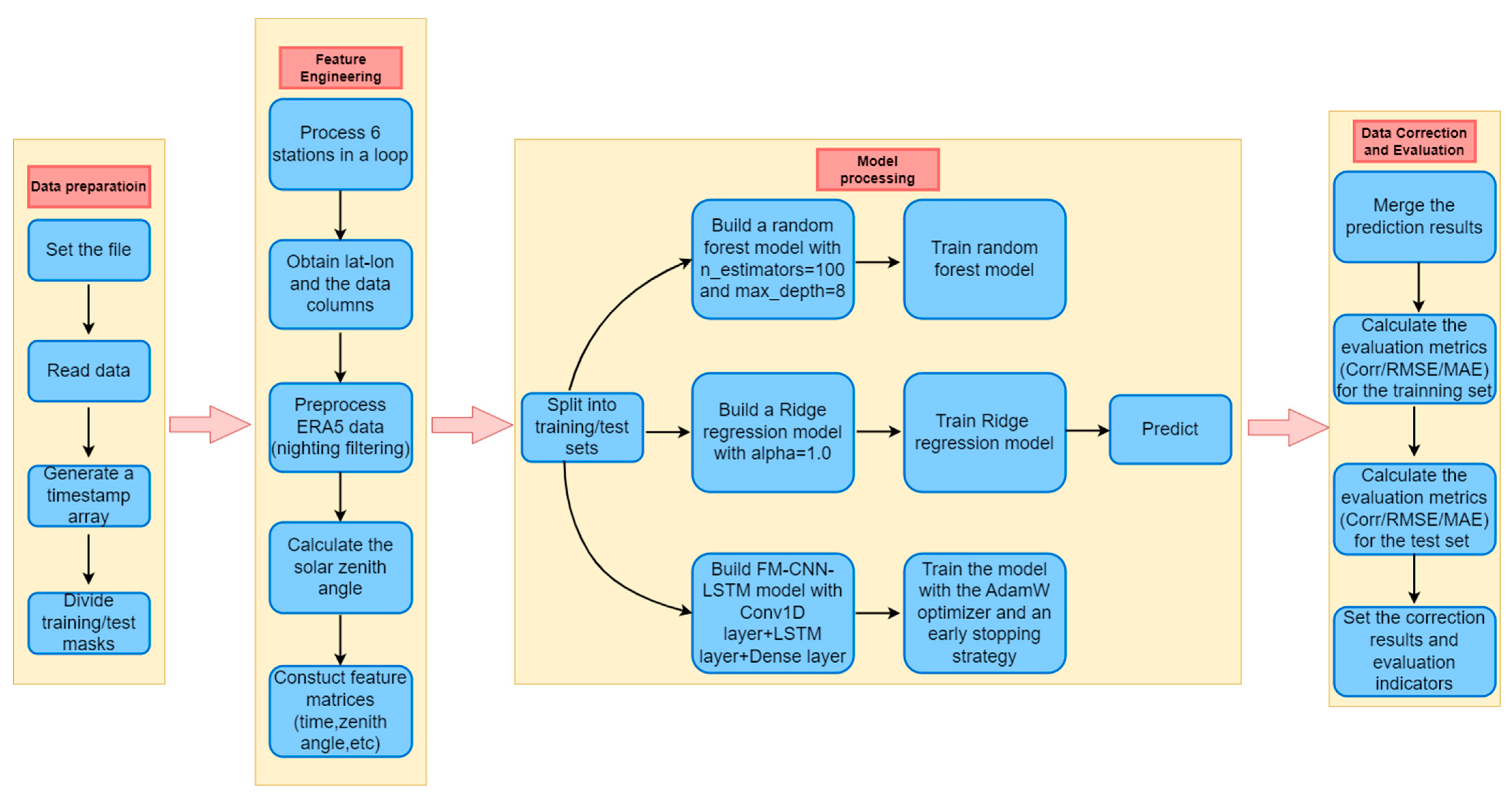
Figure 2 presents a detailed workflow illustrating the data correction procedure implemented in this study. The workflow comprises four main stages: data preparation, feature engineering, model processing, and data correction and evaluation. Firstly, the raw data files are imported, read, and structured into timestamp arrays, followed by partitioning into training and test subsets. Subsequently, in the feature engineering phase, data from six observational stations are processed to extract relevant spatial (e.g., latitude and longitude), temporal, and solar geometry features. Specifically, solar zenith angles are computed after excluding nighttime data from the ERA5 reanalysis dataset. These extracted features form the input matrices for model training. The model processing phase involves splitting the prepared datasets into training and test sets, upon which three distinct models—Random Forest (with parameters: n_estimators = 100 and max_depth = 8), Ridge regression (alpha = 1.0), and an advanced FM-CNN-LSTM model (consisting of a Conv1D layer, an LSTM layer, and a Dense output layer)—are constructed, trained, and subsequently utilized for predictions. The FM-CNN-LSTM model employs the AdamW optimizer and an early-stopping strategy to enhance training efficiency and performance. Finally, the prediction results are merged and evaluated using metrics such as the correlation coefficient, root mean square error, and mean absolute error for both training and test sets. The corrected datasets, along with evaluation metrics, are then stored for subsequent analysis.

2.2.2. Evaluation Metrics

In this study, Pearson’s correlation coefficient (CC), root mean square error (RMSE), and mean absolute error (MAE) are used to evaluate the accuracy of the ERA5 shortwave radiation data both before and after applying the corrections.
The CC measures the degree of linear correlation between two variables, with values ranging from −1 to 1. A value of 1 indicates a perfect positive correlation, −1 indicates a perfect negative correlation, and 0 denotes no linear correlation. When evaluating the consistency between observed and ERA5 reanalysis data, this coefficient quantifies the degree to which their trends align. The formula is expressed as follows:
R = i = 1 N ( E i E ¯ ) ( Q i O ¯ ) i = 1 N ( E i E ¯ ) 2 i = 1 N ( O i O ¯ ) 2
The RMSE is a widely used metric to quantify the differences between observed and predicted (or reanalyzed) data, representing the average magnitude of deviations. A lower RMSE indicates better accuracy and closer agreement between the observed data and ERA5 values. The RMSE calculation is expressed as:
R M S E = 1 N i = 1 N ( E i O i ) 2
The MAE calculates the average of the absolute differences between observed values and corresponding ERA5 data points, offering a straightforward measure of average deviation. Unlike RMSE, MAE is less sensitive to outliers because it assigns equal weight to all errors rather than disproportionately penalizing larger errors. The MAE formula is as follows:
M A E = 1 N i = 1 N ( | E i O i | )
Here, E i and O i represent the ERA5 data series and the observation data, respectively, while E ¯ and O ¯ denote the mean values of each dataset.

3. Results

3.1. Evaluation of the ERA5 Dataset

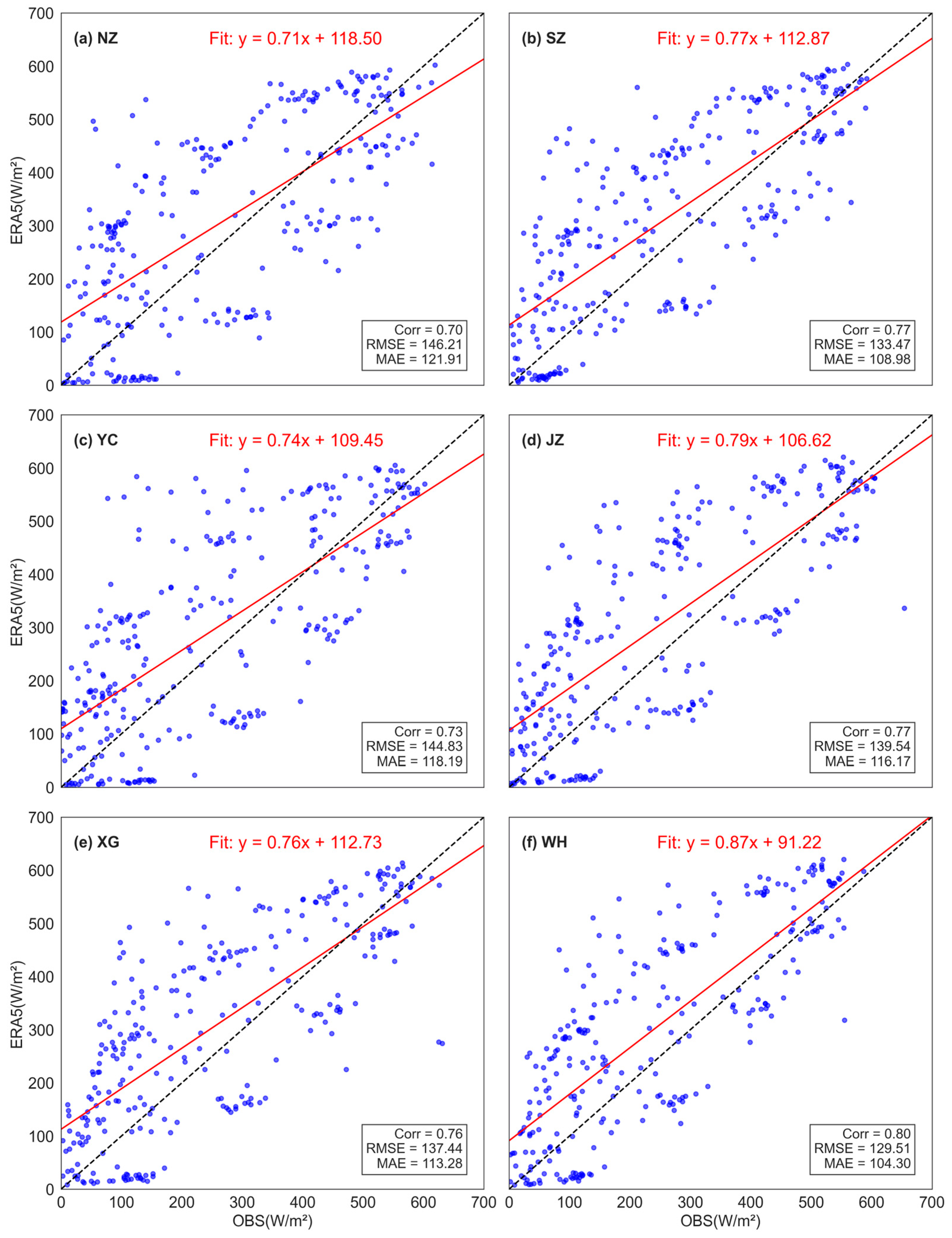
Overall, the CC between observed and ERA5 shortwave radiation ranged from 0.78 to 0.83, indicating relatively consistent performance across the studied stations. RMSE varied from 157.08 to 175.99 W/m2, while mean absolute errors (MAE) ranged from 122.37 to 139.53 W/m2, further suggesting modest variability in error magnitudes among the stations. Nonetheless, clear distinctions were observed. Specifically, XG and WH stations exhibited the highest CC (0.82 and 0.83, respectively), implying that ERA5 data had the strongest agreement with observations at these locations. In contrast, the NZ station showed the lowest correlation coefficient (0.78), reflecting comparatively weaker performance of the ERA5 data. Correspondingly, NZ station had the largest RMSE (175.99 W/m2) and MAE (139.53 W/m2), while WH displayed the smallest RMSE (157.08 W/m2) and MAE (122.37 W/m2), indicating that the ERA5 data most accurately captured observed radiation conditions at WH (Figure 3).
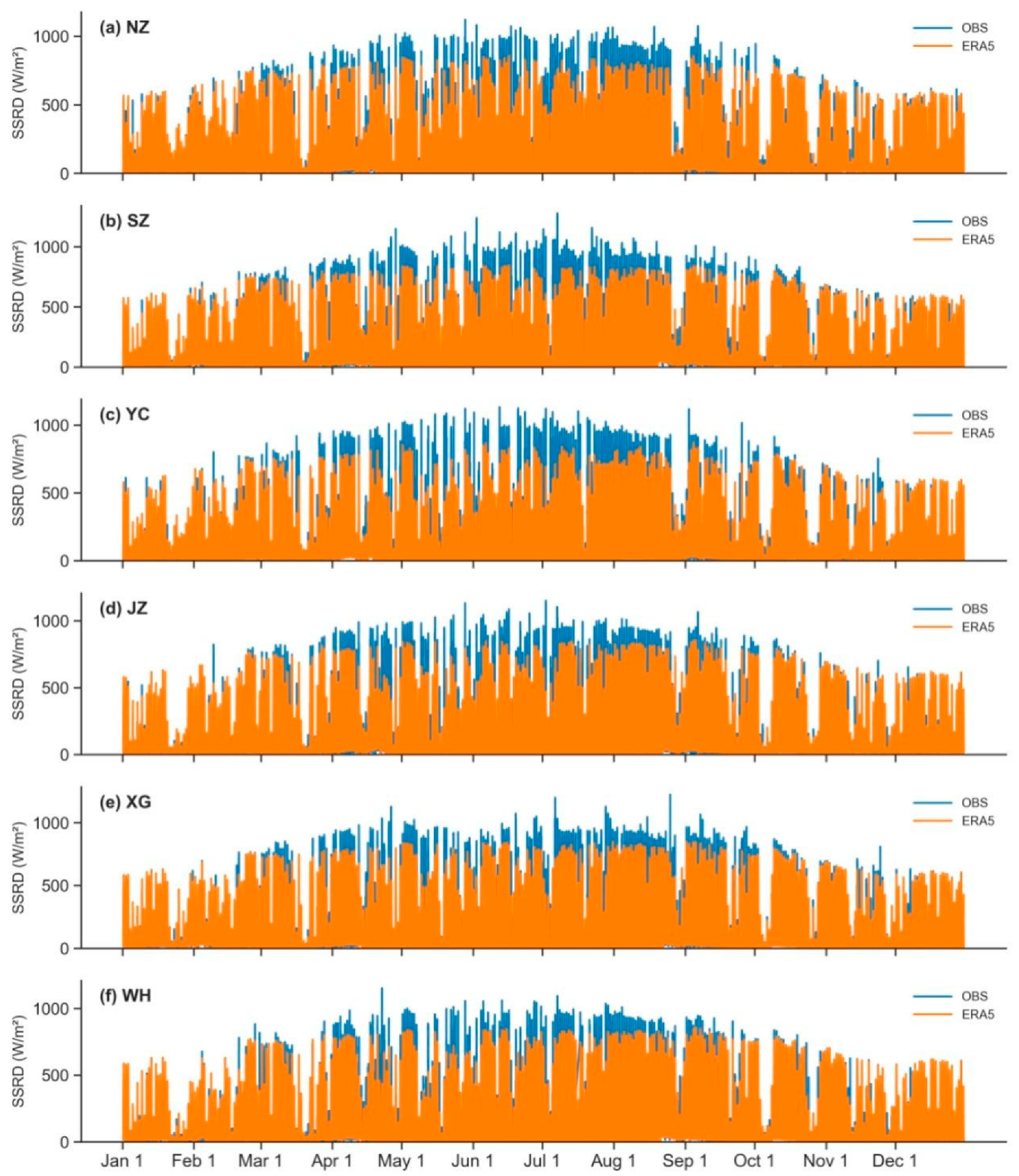
Hourly analysis (Figure 4) further revealed that ERA5 data consistently underestimated shortwave radiation during summer and overestimated it during winter at all stations, achieving optimal accuracy in autumn. Specifically, October exhibited the highest CC, accompanied by the lowest RMSE and MAE, indicating the strongest agreement and smallest errors between ERA5 reanalysis and observed shortwave radiation. Conversely, July had the lowest CC and the highest RMSE and MAE values, demonstrating the weakest correlation and greatest discrepancies between ERA5 data and observations.
These results indicate that ERA5 generally performs better in regions characterized by lower elevations and relatively simple topography, while its performance tends to degrade in more topographically complex areas such as the NZ station. This variability likely arises from the pronounced impact of local terrain features on solar radiation in complex terrains, combined with the inherent limitations of reanalysis datasets in accurately resolving small-scale topographic variations. Additionally, the observed seasonal variation in performance is likely related to differences in atmospheric stability and meteorological complexity, with relatively stable conditions in spring and autumn (particularly October) leading to enhanced accuracy, while complex and variable summer conditions (particularly July) result in increased uncertainties. In winter, extensive cloud coverage and low sun angles may further affect the accuracy of ERA5 estimates.

3.2. Results Based on the Ridge Regression Model

We applied Ridge Regression, trained with observational data from January to November 2022, to correct biases in the ERA5 shortwave radiation dataset. The corrected ERA5 data demonstrated clear improvements over the original dataset, exhibiting better consistency with observed values. Specifically, correlation coefficients increased by approximately 4.70% to 8.00% across the six stations, while the RMSE and MAE decreased by about 12.09–14.82% and 14.21–17.80%, respectively (Table 2). These improvements suggest that Ridge Regression effectively enhances ERA5 data accuracy for practical solar radiation applications.
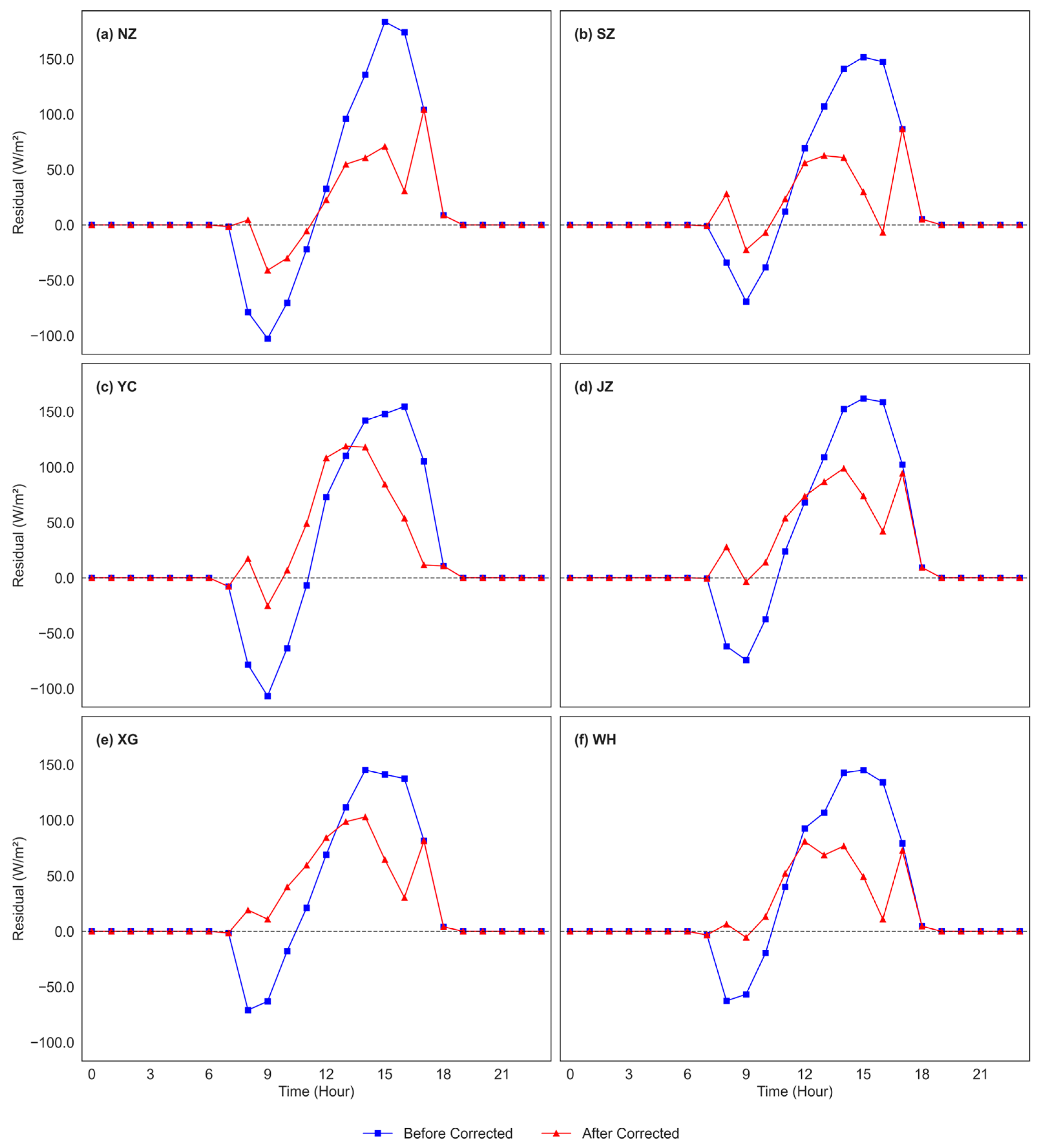
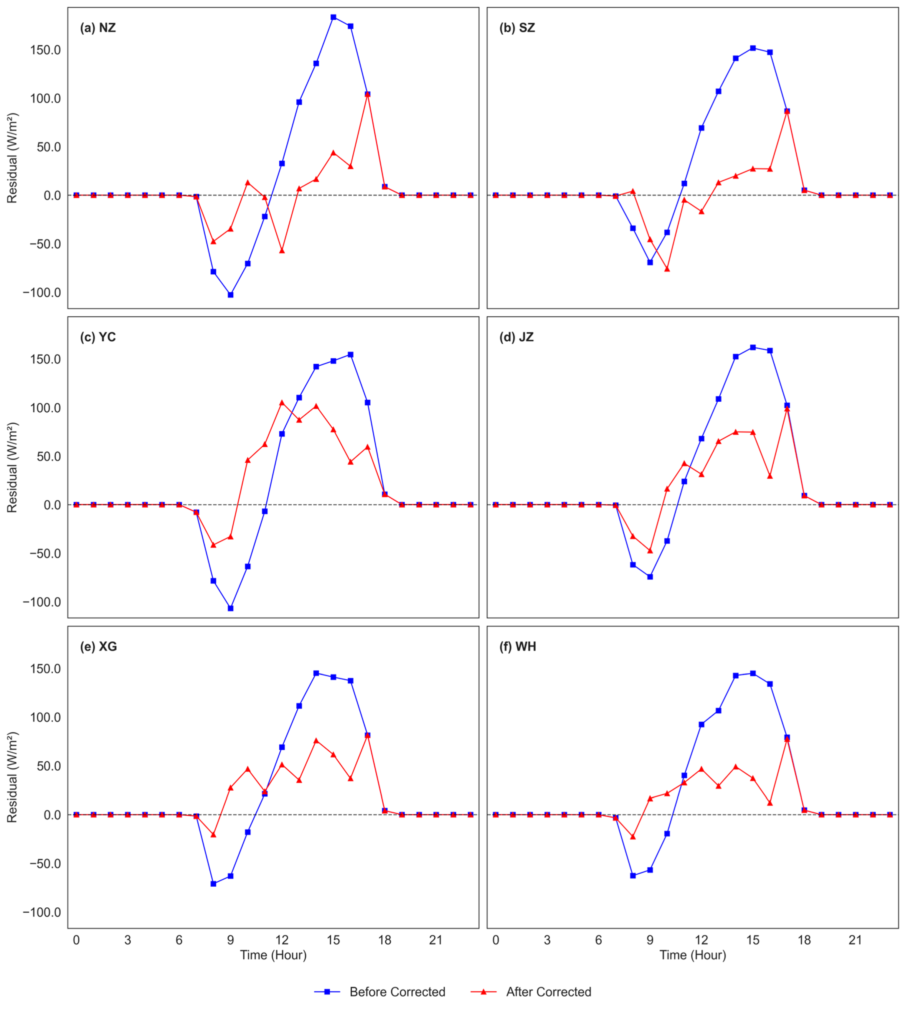
Data from December 2022 were used for model validation. Across all stations, the original ERA5 data show a consistent overestimation of peak shortwave radiation during midday hours (typically 11:00–14:00 LT), with residuals reaching 140–160 W/m2 at stations such as NZ (Figure 5a), YC (Figure 5c), and WH (Figure 5f). Morning hours (around 8:00–10:00 LT) exhibit systematic underestimation with negative residuals often below −50 W/m2. These biases reflect a diurnal asymmetry in the original ERA5 estimates. After applying Ridge Regression, the magnitude of residuals is significantly reduced. Peak residuals during midday hours decrease to within ±50 W/m2 across most stations, and early morning underestimations are similarly mitigated. For instance, at the WH station (panel f), the midday residual decreases from ~150 W/m2 before correction to ~60 W/m2 after correction. Likewise, the sharp negative bias around 9:00 LT is corrected from approximately −90 W/m2 to values closer to −20 W/m2. Overall, the corrected data (red lines) exhibit flatter and more symmetrical residual curves, indicating improved alignment with observed radiation patterns throughout the diurnal cycle. These results quantitatively demonstrate the effectiveness of Ridge Regression in reducing time-dependent biases in ERA5 shortwave radiation.
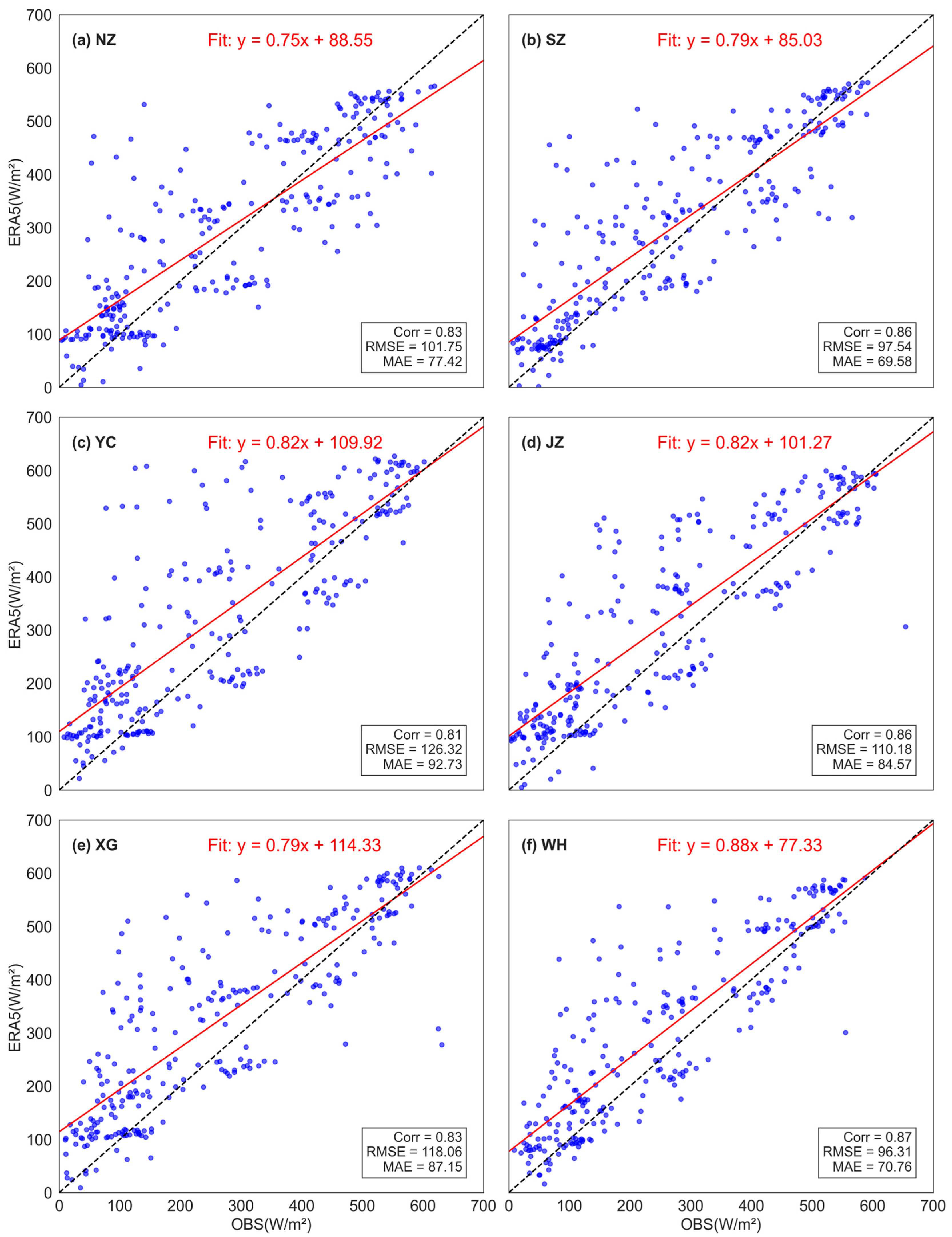
Scatter plots and statistical analyses (Figure 6 and Figure 7) quantitatively confirm these qualitative observations. Before correction (Figure 6), correlation coefficients between observed and ERA5 data ranged from 0.70 (NZ) to 0.80 (WH), reflecting moderate yet clear discrepancies. Correspondingly, RMSE varied from 129.51 W/m2 (WH) to 146.21 W/m2 (NZ), and MAE ranged from 104.30 W/m2 (WH) to 121.91 W/m2 (NZ). Linear regression slopes, consistently below unity (0.71–0.87), further indicated systematic biases, demonstrating ERA5’s tendency to underestimate variability in peak radiation and overestimate values during low-radiation conditions. After implementing the Ridge Regression correction (Figure 7), statistical metrics improved markedly across all stations. Specifically, correlation coefficients significantly increased, notably at the WH station (from 0.80 to 0.87), indicating enhanced alignment with observational data. RMSE and MAE values were substantially reduced; for example, at WH, RMSE decreased from 129.51 to 96.31 W/m2 and MAE declined from 104.30 to 70.76 W/m2, highlighting pronounced improvements in accuracy. Regression slopes also approached unity (0.75–0.88), signifying better representation of observed solar radiation variability.
Despite these improvements, slight residual biases persisted, particularly during periods of rapidly fluctuating radiation conditions, underscoring the necessity for further methodological refinements. Overall, the results affirm the effectiveness of the Ridge Regression correction method in significantly reducing inherent biases within the ERA5 dataset, substantially improving its reliability. Nonetheless, further enhancements, possibly through integrating additional predictors or employing advanced modeling frameworks, remain essential to achieve greater accuracy under complex atmospheric conditions.

3.3. Results Based on the Random Forest Model

Figure 8 shows the average hourly residuals between corrected ERA5 shortwave radiation and ground-based observations before (blue lines) and after (red lines) correction using the Random Forest model. After applying the Random Forest correction, residuals are substantially reduced across all hours and stations. Notably, the Random Forest method effectively flattens the residual curves, with peak errors generally reduced to within ±50 W/m2, and morning underestimations substantially mitigated. When compared to the Ridge Regression results shown in Figure 5, Random Forest demonstrates a more robust correction capacity, yielding smoother diurnal profiles and smaller residual amplitudes across all sites. These improvements underscore Random Forest’s superior ability to model complex, nonlinear interactions influencing surface radiation, making it more effective than linear methods in addressing ERA5 biases under varying atmospheric and topographic conditions.
Scatter plots and statistical comparisons depicted in Figure 7 and Figure 9 further support these improvements. The ERA5 data corrected using the Random Forest method align more closely with observations, as indicated by higher correlation coefficients (up to 0.88), lower RMSE (as low as 86.14 W/m2 at WH), and smaller MAE values (e.g., 60.05 W/m2 at WH). The regression slopes also approach unity more consistently than those in Figure 7, which shows the Ridge Regression results. For example, at the WH station, the slope is 0.84 with Random Forest compared to 0.88 with Ridge, yet Random Forest achieves significantly lower RMSE and MAE, indicating a better trade-off between accuracy and bias reduction. In contrast, Ridge Regression exhibits larger residual scatter and more systematic overestimations or underestimations at several stations.
These results highlight the effectiveness and clear superiority of the Random Forest correction method in significantly improving ERA5-derived solar radiation estimates. This method offers a more accurate depiction of diverse atmospheric conditions while indicating areas for future refinement.

3.4. Results Based on the FMCNN-LSTM Model

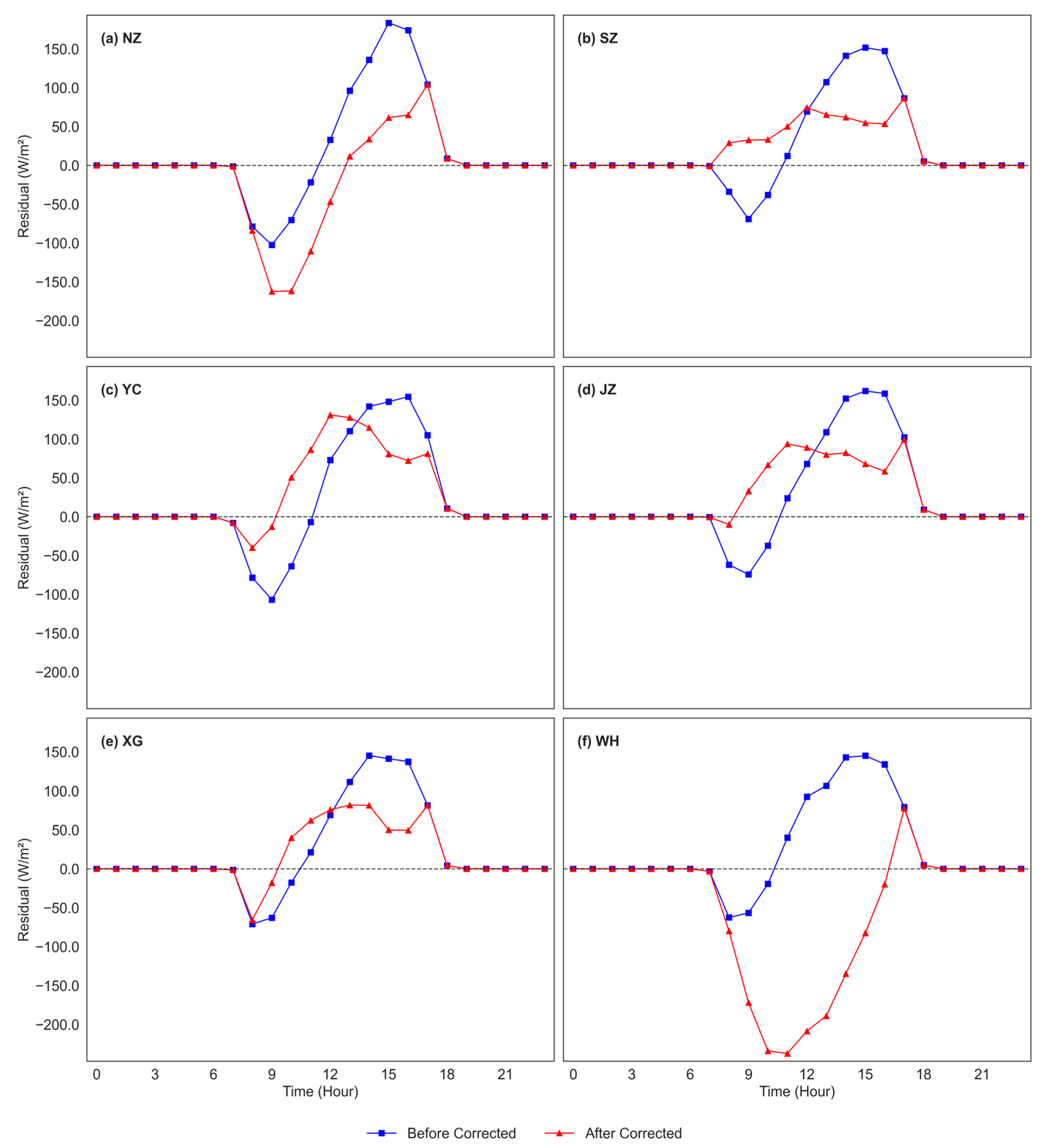
Results based on the FMCNN-LSTM model are presented in Figure 10 and Figure 11. After applying the FM-CNN-LSTM correction, the ERA5 dataset shows overall improvement, but the correction performance varies significantly among stations (Figure 10). Stations such as SZ and JZ exhibit notably better agreement between the corrected ERA5 data and ground-based observations. However, substantial discrepancies remain at WH, where the corrected values severely underestimate observed radiation, especially during peak solar hours. This inconsistency reflects the FM-CNN-LSTM model’s limited ability to generalize correction performance across diverse atmospheric and topographic conditions, particularly when compared to other methods.
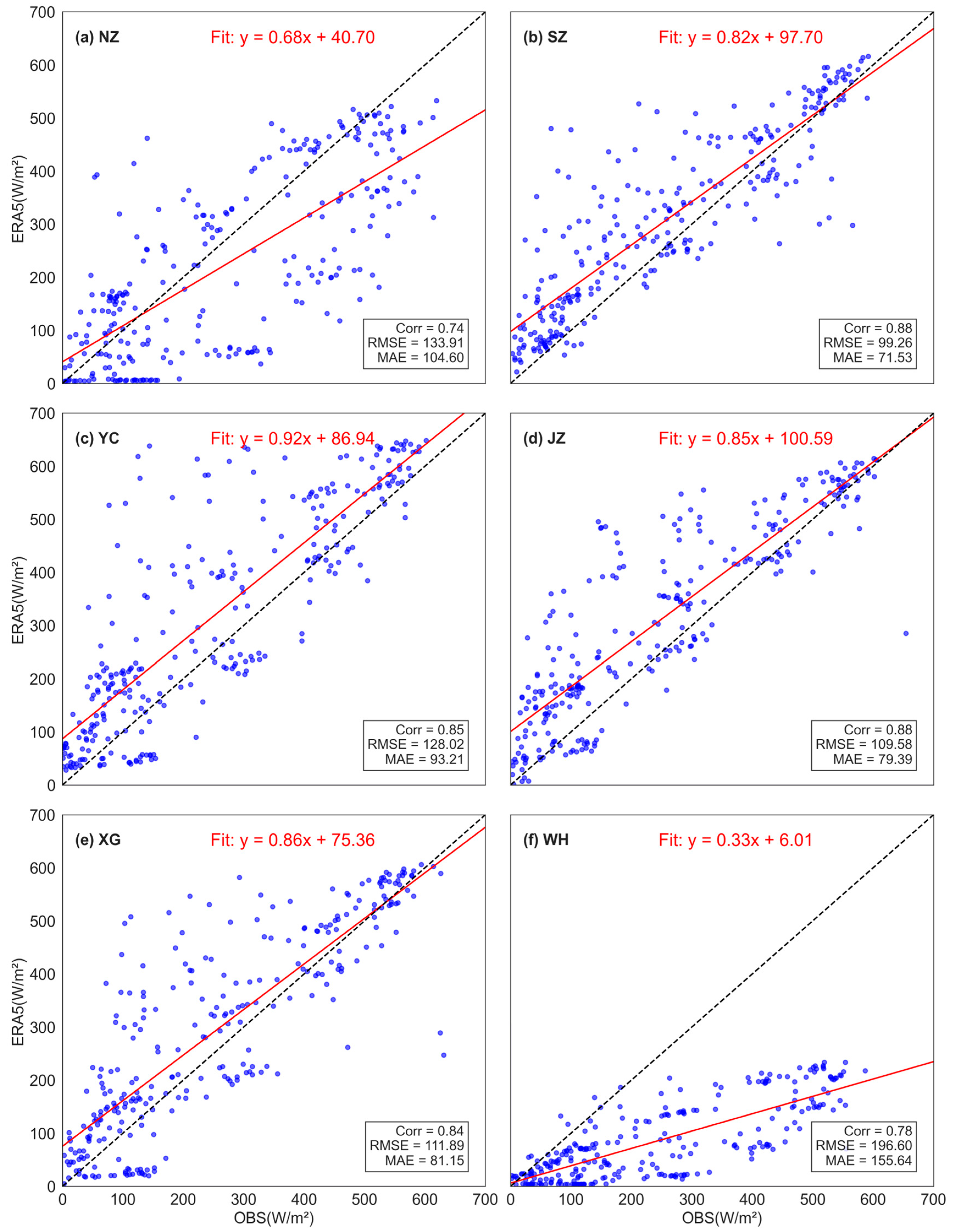
As shown in Figure 11, the FM-CNN-LSTM method yielded statistical improvements at stations SZ, YC, JZ, and XG, with correlation coefficients reaching up to 0.88 at SZ and JZ, and noticeable reductions in RMSE and MAE. In contrast, at WH, the model’s performance deteriorates considerably, with the correlation coefficient dropping to 0.78 and RMSE and MAE increasing to 196.60 W/m2 and 155.64 W/m2, respectively, which is the worst performance among all stations. Compared to previously discussed methods, particularly the Random Forest model (Figure 9), FM-CNN-LSTM delivers less stable and less reliable results. The Random Forest approach demonstrates superior and more consistent performance across all stations, effectively reducing systematic biases.
In summary, while the FM-CNN-LSTM method enhances the ERA5 data accuracy relative to the original dataset, its performance is inconsistent across stations and inferior overall compared to the Random Forest method. These findings highlight the effectiveness and reliability of the Random Forest approach as the preferred correction method, while also identifying critical limitations and areas for potential improvement within the FM-CNN-LSTM methodology.

3.5. Comparison of the Three Correction Methods

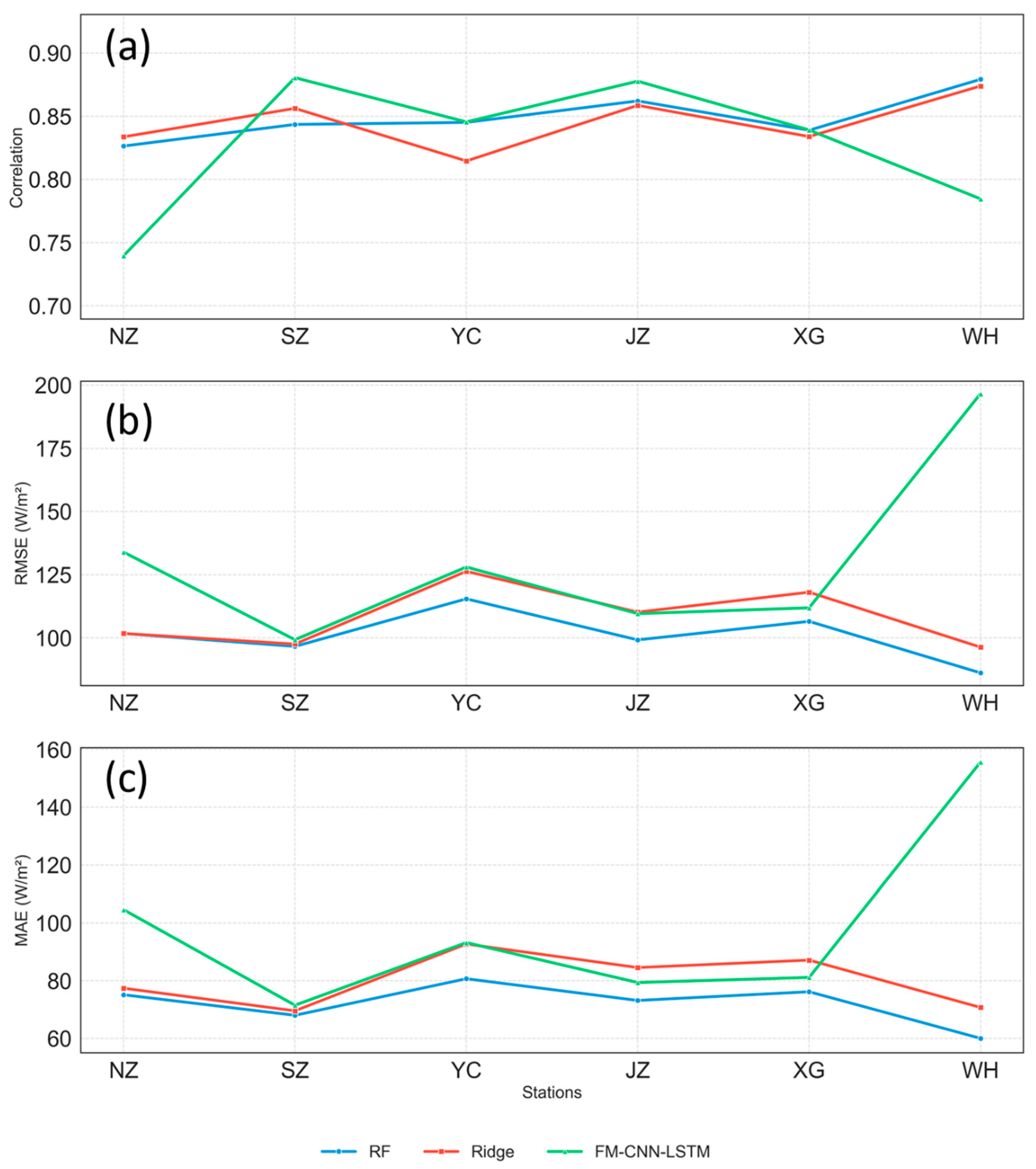
Figure 12 presents a quantitative comparison of three correction methods, Random Forest, Ridge regression, and FM-CNN-LSTM, in terms of CC, RMSE, and MAE for corrected ERA5 solar radiation data at six observational stations. The CC values are generally highest using the Random Forest method, consistently ranging between approximately 0.84 and 0.88, with the highest correlation (0.88) observed at the WH station. By comparison, Ridge Regression displays slightly lower correlation coefficients, typically within the range of 0.83–0.87, while FM-CNN-LSTM exhibits greater variability, with values ranging significantly from 0.74 (NZ) to 0.88 (SZ). Moreover, the Random Forest method consistently achieves the lowest RMSE values across all stations, notably at WH (86.14 W/m2). Ridge Regression closely follows RF, showing marginally higher yet stable RMSE values across all stations. Conversely, FM-CNN-LSTM demonstrates substantial variability in RMSE, particularly a high RMSE of 196.60 W/m2 at WH, reflecting significant inconsistency at this site. Similarly, in terms of MAE (Figure 12c), the Random Forest method consistently outperforms the other two methods, maintaining the lowest MAE values, ranging from approximately 60.05 W/m2 (WH) to about 80.70 W/m2 (YC). Ridge Regression again closely follows RF, exhibiting slightly higher MAE values. In contrast, FM-CNN-LSTM reveals substantial discrepancies and lower consistency, especially evident at WH with an exceptionally high MAE of 155.64 W/m2.
These comparative results objectively demonstrate that the Random Forest correction method provides the most consistent and robust improvement across all evaluation metrics and observational stations, surpassing Ridge regression and FM-CNN-LSTM methods. FM-CNN-LSTM, despite demonstrating strong potential at selected stations, reveals significant variability and reduced reliability, emphasizing the superior effectiveness and robustness of the Random Forest approach in correcting ERA5 solar radiation data.

3.6. Spatial Distribution of the Radiation over Hubei Province

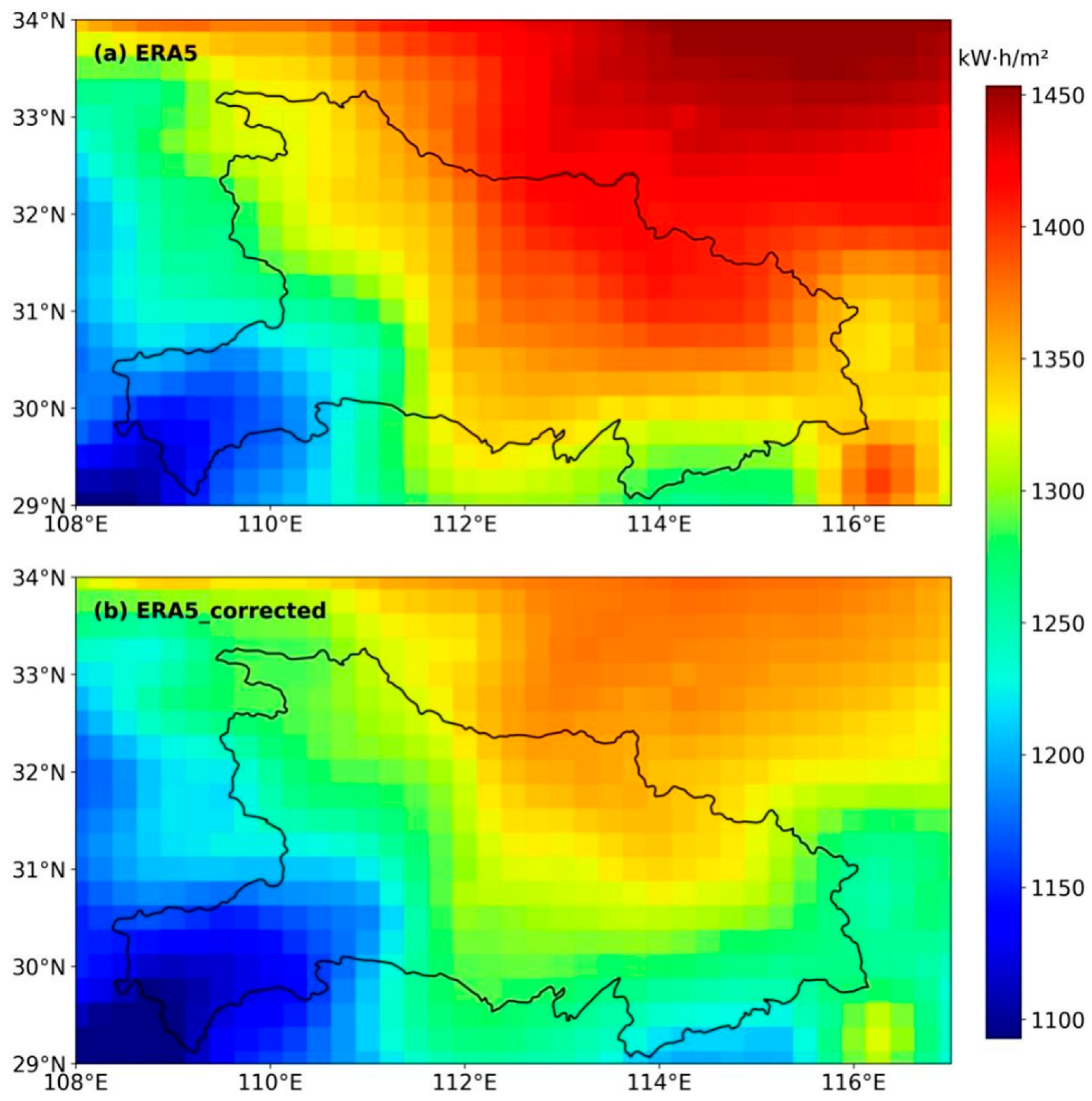
Since the Random Forest method exhibited superior performance in correcting ERA5 shortwave radiation data, we applied this method to the ERA5 dataset over Hubei Province. Figure 13 illustrates the spatial distribution of annual cumulative shortwave radiation across Hubei Province for the year 2022, contrasting the original ERA5 dataset (Figure 13a) with the dataset corrected using the Random Forest approach (Figure 13b). Before correction, ERA5 data tend to present a relatively homogeneous and overly high distribution of radiation, particularly in eastern and northeastern areas, where values exceed 1400 kWh/m2 in many regions. After correction, the radiation distribution patterns exhibit more detailed spatial patterns, clearly reflecting a logical west-to-east gradient shaped by the province’s topography. Specifically, radiation values are comparatively lower (approximately 1100–1150 kWh/m2) in the mountainous and hilly terrains of southwestern Hubei, likely due to increased cloud cover and complex topographic shading effects. In contrast, the northeastern plains and southeastern regions displayed notably higher radiation levels, typically ranging from 1250 to 1350 kWh/m2, with localized peak values exceeding 1350 kWh/m2, particularly in the eastern parts.
According to solar photovoltaic industry standards, areas receiving annual solar radiation of approximately 1300 kWh/m2 or higher are classified as rich in solar resources, thus suitable for large-scale photovoltaic power generation. Consequently, the corrected radiation dataset clearly identifies eastern and northeastern regions of Hubei Province as particularly advantageous for photovoltaic energy development. These refined spatial assessments underscore the practical importance of employing sophisticated statistical correction methods, such as the Random Forest model, to provide highly accurate and reliable solar radiation datasets. Such methodological improvements substantially enhance the quality and precision of solar energy planning and investment decisions, offering valuable insights and robust guidance to stakeholders in the photovoltaic industry.

4. Summary and Discussion

The present study evaluated and compared the performance of three distinct bias correction methods, Ridge Regression, Random Forest, and FM-CNN-LSTM, using observational data from six photovoltaic stations in Hubei Province, China, to improve ERA5-derived shortwave solar radiation estimates. The findings clearly demonstrated the necessity and effectiveness of bias correction, highlighting systematic biases in the original ERA5 dataset, especially overestimations of peak radiation (approximately 50–100 W/m2 at stations such as Wuhan (WH) and Yichang (YC) stations and underestimations during cloudy or low-radiation conditions.
Quantitative assessments showed that all correction methods enhanced ERA5 radiation estimates compared to the original data. Among these, the Random Forest method consistently outperformed the other two, exhibiting the highest correlation coefficients (0.84–0.88), and lowest RMSE (86.14 W/m2 at WH) and MAE (60.05 W/m2 at WH). Ridge Regression also delivered consistent but slightly lower improvements, increasing correlations by approximately 4.7–8.0% and reducing RMSE and MAE by 12.1–14.8% and 14.2–17.8%, respectively. Conversely, FM-CNN-LSTM, despite strong performance at certain stations (e.g., correlation of 0.88 at Suizhou station), showed considerable inconsistency and limited generalization, notably at WH, where RMSE and MAE sharply increased to 196.60 W/m2 and 155.64 W/m2, respectively.
Applying the Random Forest model to the entire Hubei Province further demonstrated its practical advantages by significantly refining the spatial representation of solar radiation. The corrected data exhibited a realistic spatial gradient influenced by terrain complexity, with annual radiation ranging from approximately 1100 to 1150 kWh/m2 in the mountainous southwest to above 1350 kWh/m2 in the northeastern plains. Areas exceeding 1300 kWh/m2 are highly favorable for large-scale photovoltaic installations, highlighting eastern and northeastern Hubei as key regions for solar development.
In summary, our results reaffirm that Random Forest is a highly effective tool for correcting ERA5 solar radiation biases. Consistent evidence of Random Forest’s strong performance has been reported in diverse climate regions, e.g., Norway [28], France [29], and North America [30], where it delivers both high accuracy and robustness. Nevertheless, Random Forest is not universally superior. Region-specific evaluations show that model ranking shifts with local climate: Random Forest often excels in very humid environments, whereas Support Vector Machines (SVM) or Multi-Layer Perceptrons (MLP) can outperform Random Forest in arid or temperate zones. Moreover, compared to traditional or single-tree methods, Random Forest offers significant improvements, but under data-rich or highly nonlinear conditions (e.g., regions with complex topography), well-tuned gradient boosting methods, SVM, or deep learning models may yield better performance [31,32,33,34]. Similar patterns hold for other surface variables such as temperature, precipitation, and evapotranspiration [35,36], underscoring that no single algorithm dominates in every context.
These findings suggest that future work may explore the integration of bias correction with spatial downscaling techniques to better capture local variability, especially in regions with complex topography. Such a combined approach would help refine the spatial granularity of radiation estimates. In addition, due to the limited availability and quality of long-term ground-based solar radiation observations, this study was restricted to the year 2022, which offered the most complete dataset across all stations. While this ensured high data integrity, it also limited the temporal representativeness of the analysis, highlighting the importance of incorporating extended multi-year datasets in future research.

Author Contributions

C.X.: Methodology, software, investigation, validation, writing original draft preparation. M.J.: Formal analysis, data gathering, review, and editing. M.W.: Conceptualization, supervision, validation, review, and editing. All authors have read and agreed to the published version of the manuscript.

Funding

This research was funded by the National Key R&D Plan “Inter-governmental International Science & Technology Innovation Cooperation” Key Specialized Program [2023YFE0112700]. And the APC was funded by the National Key R&D Plan “Inter-governmental International Science & Technology Innovation Cooperation” Key Specialized Program (2023YFE0112700). Sichuan Science and Technology Program (2024NSFSC0776), Hubei Provincial Natural Science Foundation (2023AFB543) and National Key R&D Program of China (2024YFF0809204).

Institutional Review Board Statement

Not applicable.

Informed Consent Statement

Not applicable.

Data Availability Statement

The original contributions presented in this study are included in the article. Further inquiries can be directed to the corresponding author.

Conflicts of Interest

At the time of writing, Chiyu Xian and Minghong Jin are employees of Southwest Electric Power Design Institute Co., Ltd., and all their work is performed on a volunteer and pro bono basis. The remaining authors do not have conflicts to declare.

References

  1. Chodakowska, E.; Nazarko, J.; Nazarko, Ł.; Rabayah, H.S. Solar radiation forecasting: A systematic meta-review of current methods and emerging trends. Energies 2024, 17, 3156. [Google Scholar] [CrossRef]
  2. Li, P.; Gao, X.; Li, Z.; Ye, T.; Zhou, X. Effects of fishery complementary photovoltaic power plant on near-surface meteorology and energy balance. Renew. Energy 2022, 187, 698–709. [Google Scholar] [CrossRef]
  3. Antonanzas, J.; Osorio, N.; Escobar, R.; Urraca, R.; Martinez-de-Pison, F.J.; Antonanzas-Torres, F. Review of photovoltaic power forecasting. Sol. Energy 2016, 136, 78–111. [Google Scholar] [CrossRef]
  4. Voyant, C.; Notton, G.; Kalogirou, S.; Nivet, M.L.; Paoli, C.; Motte, F.; Fouilloy, A. Machine learning methods for solar radiation forecasting: A review. Renew. Energy 2017, 105, 569–582. [Google Scholar] [CrossRef]
  5. Adomako, A.B.; Jamshidi, E.J.; Yusup, Y.; Elsebakhi, E.; Jaafar, M.H.; Ishak, M.I.S.; Lim, H.S.; Ahmad, M.I. Deep learning approaches for bias correction in WRF model outputs for enhanced solar and wind energy estimation: A case study in East and West Malaysia. Ecol. Inform. 2024, 84, 102898. [Google Scholar] [CrossRef]
  6. Diagne, M.; David, M.; Lauret, P.; Boland, J.; Schmutz, N. Review of solar irradiance forecasting methods and a proposition for small-scale insular grids. Renew. Sustain. Energy Rev. 2013, 27, 65–76. [Google Scholar] [CrossRef]
  7. Hersbach, H.; Bell, B.; Berrisford, P.; Hirahara, S.; Horányi, A.; Muñoz-Sabater, J.; Nicolas, J.; Peubey, C.; Radu, R.; Schepers, D.; et al. The ERA5 global reanalysis. Q. J. R. Meteorol. Soc. 2020, 146, 1999–2049. [Google Scholar] [CrossRef]
  8. Wang, H.; Wang, Y. Evaluation of the Accuracy and Trend Consistency of Hourly Surface Solar Radiation Datasets. Remote Sens. 2025, 17, 1317. [Google Scholar] [CrossRef]
  9. Zhang, J.; Gao, Z.; Li, Y. Deep-learning correction methods for weather research and forecasting (WRF) model precipitation forecasting: A case study over Zhengzhou, China. Atmosphere 2024, 15, 631. [Google Scholar] [CrossRef]
  10. Yang, D.; Bright, J.M. Worldwide validation of satellite-derived and reanalysis solar radiation products. Sol. Energy 2020, 210, 3–19. [Google Scholar] [CrossRef]
  11. He, Y.; Yang, K.; Ren, Y.; Zou, M.; Yuan, X.; Tang, W. Causes of the extremely low solar radiation in the 2021 growing season over southeastern Tibetan Plateau and its impact on vegetation growth. Bull. Am. Meteorol. Soc. 2023, 104, E359–E366. [Google Scholar] [CrossRef]
  12. King, F.; Erler, A.R.; Frey, S.K.; Fletcher, C.G. Application of machine learning techniques for regional bias correction of snow water equivalent estimates in Ontario, Canada. Hydrol. Earth Syst. Sci. 2020, 24, 4887–4902. [Google Scholar] [CrossRef]
  13. Barbieri, F.; Rajakaruna, S.; Ghosh, A. Very short-term photovoltaic power forecasting with cloud modeling: A review. Renew. Sustain. Energy Rev. 2017, 75, 242–263. [Google Scholar] [CrossRef]
  14. Cui, X.; Liu, C.; Shan, L.; Lin, J.; Zhang, J.; Jiang, Y.; Zhang, G. Spatial-Temporal responses of ecosystem services to land use transformation driven by rapid urbanization: A case study of Hubei Province, China. Int. J. Environ. Res. Public Health 2021, 19, 178. [Google Scholar] [CrossRef] [PubMed]
  15. Chu, Y.; Li, M.; Coimbra, C.F.; Feng, D.; Wang, H. Intra-hour irradiance forecasting techniques for solar power integration: A review. iScience 2021, 24, 103136. [Google Scholar] [CrossRef] [PubMed]
  16. Dormann, C.F.; Elith, J.; Bacher, S.; Buchmann, C.; Carl, G.; Carré, G.; García Marquéz, J.R.; Gruber, B.; Lafourcade, B.; Leitão, P.J.; et al. Collinearity: A review of methods to deal with it and a simulation study evaluating their performance. Ecography 2013, 36, 27–46. [Google Scholar] [CrossRef]
  17. Marquardt, D.W. Generalized inverses, ridge regression, biased linear estimation, and nonlinear estimation. Technometrics 1970, 12, 591–612. [Google Scholar] [CrossRef]
  18. Hastie, T.; Tibshirani, R.; Wainwright, M. Statistical Learning with Sparsity: The Lasso and Generalizations; CRC Press: Boca Raton, FL, USA, 2015. [Google Scholar]
  19. Breiman, L. Random forests. Mach. Learn. 2001, 45, 5–32. [Google Scholar] [CrossRef]
  20. Belgiu, M.; Drăguţ, L. Random forest in remote sensing: A review of applications and future directions. ISPRS J. Photogramm. Remote Sens. 2016, 114, 24–31. [Google Scholar] [CrossRef]
  21. Rodriguez-Galiano, V.F.; Sanchez-Castillo, M.; Chica-Olmo, M.; Chica-Rivas, M. Machine learning predictive models for mineral prospectivity: An evaluation of neural networks, random forest, regression trees and support vector machines. Ore Geol. Rev. 2015, 71, 804–818. [Google Scholar] [CrossRef]
  22. Tyralis, H.; Papacharalampous, G.; Langousis, A. A brief review of random forests for water scientists and practitioners and their recent history in water resources. Water 2019, 11, 910. [Google Scholar] [CrossRef]
  23. Rendle, S. Factorization machines. In IEEE International Conference on Data Mining; IEEE: New York, NY, USA, 2010; pp. 995–1000. [Google Scholar]
  24. LeCun, Y.; Bengio, Y.; Hinton, G. Deep learning. Nature 2015, 521, 436–444. [Google Scholar] [CrossRef] [PubMed]
  25. Hochreiter, S.; Schmidhuber, J. Long short-term memory. Neural Comput. 1997, 9, 1735–1780. [Google Scholar] [CrossRef] [PubMed]
  26. Fu, R.; Zhang, Z.; Li, L. Using LSTM and CNN to predict stock returns based on financial news. IEEE Access 2019, 7, 156035–156044. [Google Scholar]
  27. Karim, F.; Majumdar, S.; Darabi, H.; Chen, S. LSTM fully convolutional networks for time series classification. IEEE Access 2019, 7, 1662–1669. [Google Scholar] [CrossRef]
  28. Babar, B.; Luppino, L.T.; Boström, T.; Anfinsen, S.N. Random forest regression for improved mapping of solar irradiance at high latitudes. Sol. Energy 2020, 198, 81–92. [Google Scholar] [CrossRef]
  29. Benali, L.; Notton, G.; Fouilloy, A.; Voyant, C.; Dizene, R. Solar radiation forecasting using artificial neural network and random forest methods: Application to normal beam, horizontal diffuse and global components. Renew. Energy 2019, 132, 871–884. [Google Scholar] [CrossRef]
  30. Chen, J.; Zhu, W.; Yu, Q. Estimating half-hourly solar radiation over the Continental United States using GOES-16 data with iterative random forest. Renew. Energy 2021, 178, 916–929. [Google Scholar] [CrossRef]
  31. Jia, D.; Yang, L.; Lv, T.; Liu, W.; Gao, X.; Zhou, J. Evaluation of machine learning models for predicting daily global and diffuse solar radiation under different weather/pollution conditions. Renew. Energy 2022, 187, 896–906. [Google Scholar] [CrossRef]
  32. Demir, V. Evaluation of Solar Radiation Prediction Models Using AI: A Performance Comparison in the High-Potential Region of Konya, Türkiye. Atmosphere 2025, 16, 398. [Google Scholar] [CrossRef]
  33. Huang, L.; Kang, J.; Wan, M.; Fang, L.; Zhang, C.; Zeng, Z. Solar radiation prediction using different machine learning algorithms and implications for extreme climate events. Front. Earth Sci. 2021, 9, 596860. [Google Scholar] [CrossRef]
  34. Liu, F.; Wang, X.; Sun, F.; Wang, H. Correct and remap solar radiation and photovoltaic power in China based on machine learning models. Appl. Energy 2022, 312, 118775. [Google Scholar] [CrossRef]
  35. Abdelsattar, M.; AbdelMoety, A.; Emad-Eldeen, A. Comparative analysis of machine learning techniques for temperature and humidity prediction in photovoltaic environments. Sci. Rep. 2025, 15, 15650. [Google Scholar] [CrossRef] [PubMed]
  36. Zhang, L.; Wang, Z.; Bai, X.; Zhang, H.; Liu, Y. A time-invariant bias correction strategy for improving CLM5. 0 evapotranspiration simulation by random forest method for mainland China. Atmos. Res. 2025, 324, 108196. [Google Scholar] [CrossRef]
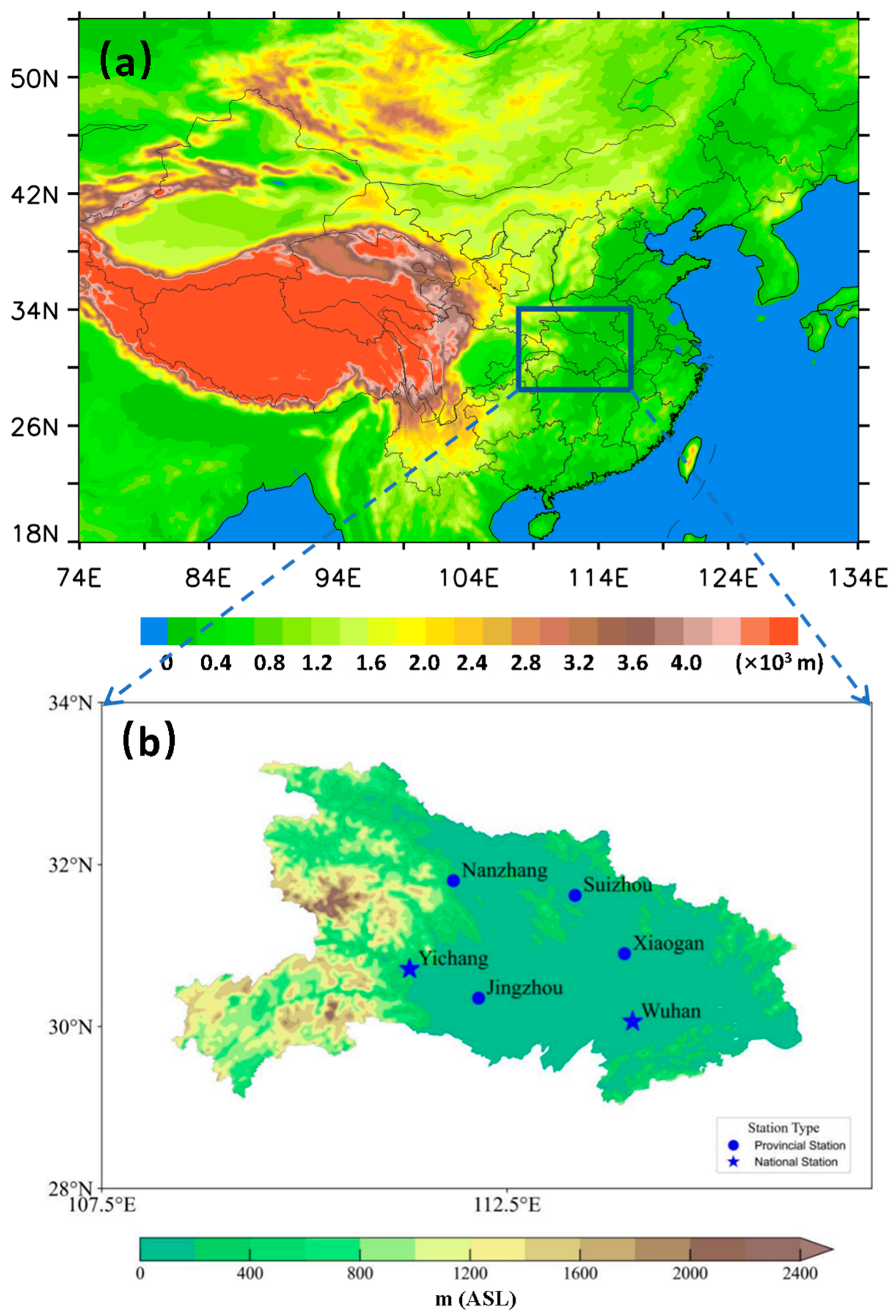
Figure 1. Geographic distribution of the six photovoltaic (PV) observation stations used in this study. (a) shows the topographic map of China, with the study area (Hubei Province) highlighted by a blue rectangle. (b) provides a detailed topographic map of Hubei Province, indicating the locations of the observation stations. The stars represent national-level stations, while the circles indicate provincial-level stations. The colors depict the topography (unit: m).
Atmosphere 16 01008 g001
Figure 2. Flowchart of the bias correction methodology employed in this study.
Atmosphere 16 01008 g002
Figure 3. Scatter plots comparing observed shortwave radiation (OBS) and ERA5 reanalysis data at six PV stations (NZ, SZ, YC, JZ, XG, WH) during 2022. The red solid lines represent linear regression fits, with corresponding equations provided at the top of each subplot. The dashed black line indicates the 1:1 reference line. Statistical metrics shown include Pearson’s correlation coefficient (Corr), root mean square error (RMSE, W/m2), and mean absolute error (MAE, W/m2).
Atmosphere 16 01008 g003
Figure 4. Hourly variations of surface shortwave radiation from observations (OBS, blue lines) and ERA5 reanalysis data (orange lines) at six PV stations (NZ, SZ, YC, JZ, XG, and WH) across Hubei Province during the year 2022.
Atmosphere 16 01008 g004
Figure 5. Average hourly differences between observed shortwave radiation and ERA5 reanalysis data at six PV stations (NZ, SZ, YC, JZ, XG, and WH) during the validation period (December 2022). The blue lines represent the residuals between observed values and the original ERA5 data (before correction), while the red lines represent the residuals after applying Ridge Regression (corrected ERA5 data).
Atmosphere 16 01008 g005
Figure 6. Scatter plots comparing observed shortwave radiation (OBS) with ERA5 reanalysis data during December 2022 at six PV stations (NZ, SZ, YC, JZ, XG, WH). The red dashed lines represent linear regression fits between corrected ERA5 and observed data, with corresponding regression equations indicated at the top of each subplot. The solid green lines represent the 1:1 reference line. Statistical evaluation metrics, including Corr, RMSE (W/m2), and MAE (W/m2), are provided in each subplot.
Atmosphere 16 01008 g006
Figure 7. Similar to Figure 6, but with the Scatter plots comparing observed shortwave radiation (OBS) with ERA5 data corrected using the Ridge Regression model.
Atmosphere 16 01008 g007
Figure 8. Similar to Figure 5, but with ERA5 data corrected using the Random Forest model.
Atmosphere 16 01008 g008
Figure 9. Similar to Figure 7, but with ERA5 data corrected using the Random Forest model.
Atmosphere 16 01008 g009
Figure 10. Similar to Figure 5, but with ERA5 data corrected using the FM-CNN-LSTM model.
Atmosphere 16 01008 g010
Figure 11. Similar to Figure 7, but with ERA5 data corrected using the FM-CNN-LSTM model.
Atmosphere 16 01008 g011
Figure 12. Comparison of correction performance for ERA5 shortwave radiation data using Random Forest (RF), Ridge Regression (Ridge), and FM-CNN-LSTM models across six PV stations (NZ, SZ, YC, JZ, XG, WH). Performance metrics include the (a) correlation coefficient (CC), (b) root mean square error (RMSE, W/m2), and (c) mean absolute error (MAE, W/m2).
Atmosphere 16 01008 g012
Figure 13. Spatial distributions of annual cumulative shortwave radiation across Hubei Province for the year 2022, comparing (a) the original ERA5 dataset and (b) the ERA5 dataset corrected using the Random Forest method.
Atmosphere 16 01008 g013
Table 1. Details of the six photovoltaic stations used in this study.
Station NameLongitudeLatitudeElevationLand Cover Type
Nanzhang (NZ)111.84° E31.80° N151.0 mForest
Suizhou (SZ)113.34° E31.62° N116.3 mCultivated land
Yichan g(YC)111.30° E30.71° N256.5 mForest
Jingzhou (JZ)112.15° E30.35° N31.8 mPaddy field
Xiaogan (XG)113.95° E30.90° N25.5 mPaddy field
Wuhan (WH)114.05° E30.06° N23.6 mPaddy field
Table 2. Correlation coefficients (CC), root mean square errors (RMSE), and mean absolute errors (MAE) between observed shortwave radiation and ERA5 reanalysis data at each radiation station for the period from January to November 2022, which was used to develop the correction models. The results based on Random Forest are underlined.
Station Correction MethodCCRMSE (W/m2)MAE (W/m2)
NZOriginal0.78177.95140.80
Ridge Regression0.85 (8.00%)151.58 (14.82%)115.73 (17.80%)
Random Forest0.91 (16.31%)117.94 (33.73%)80.240 (43.01%)
FM-CNN-LSTM0.80 (2.79%)187.88 (−5.58%)139.69 (0.79%)
SZOriginal0.81174.65136.93
Ridge Regression0.86 (6.39%)149.90 (14.17%)112.73 (17.67%)
Random Forest0.92 (13.48%)116.65 (33.21%)77.21 (43.61%)
FM-CNN-LSTM0.88 (8.54%)141.18 (19.16%)98.16 (28.32%)
YCOriginal0.81173.72134.62
Ridge Regression0.86 (5.60%)150.95 (13.11%)114.22 (15.15%)
Random Forest0.92 (13.17%)116.41 (32.99%)76.90 (42.87%)
FM-CNN-LSTM0.87 (7.73%)142.56 (17.94%)100.13 (25.62%)
JZOriginal0.80172.28133.49
Ridge Regression0.86 (5.78%)151.19 (12.24%)114.52 (14.21%)
Random Forest0.92 (13.64%)116.67 (32.28%)77.58 (41.88%)
FM-CNN-LSTM0.87 (7.52%)144.27 (16.26%)101.45 (24.00%)
XGOriginal0.82167.26130.81
Ridge Regression0.86 (4.95%)147.04 (12.09%)110.34 (15.66%)
Random Forest0.92 (11.52%)117.16 (29.96%)77.20 (40.99%)
FM-CNN-LSTM0.87 (6.03%)145.33 (13.11%)105.28 (19.52%)
WHOriginal0.83158.85123.65
Ridge Regression0.87 (4.70%)139.22 (12.36%)104.59 (15.41%)
Random Forest0.92 (11.01%)108.81 (31.50%)70.25 (43.19%)
FM-CNN-LSTM0.81 (−2.48%)311.99 (−96.41%)235.22 (−90.24%)
Disclaimer/Publisher’s Note: The statements, opinions and data contained in all publications are solely those of the individual author(s) and contributor(s) and not of MDPI and/or the editor(s). MDPI and/or the editor(s) disclaim responsibility for any injury to people or property resulting from any ideas, methods, instructions or products referred to in the content.