Abstract
We developed a microscale airflow modeling system with detailed building and terrain data to better understand the urban microclimate. Building shapes and heights, and terrain elevation data were integrated to construct a high-resolution urban surface geometry. The system, based on computational fluid dynamics using OpenFOAM, can resolve complex flow structures around built environments. Inflow boundary conditions were generated using logarithmic wind profiles derived from Automatic Weather System (AWS) observations under neutral stability. After validation with wind-tunnel data for a single block, the system was applied to airflow modeling around a university campus in Seoul using AWS data from four nearby stations. The results demonstrated that the system captured key flow characteristics such as channeling, wake, and recirculation induced by complex terrain and building configurations. In particular, easterly inflow cases with high-rise buildings on the leeward side of a mountain exhibited intensified wakes and internal recirculations, with elevated centers influenced by tall structures. This modeling framework, with further development, could support diverse urban applications for microclimate and air quality, facilitating urban resilience.
Keywords:
urban airflow; microscale modeling; CFD; OpenFOAM; GIS; Automatic Weather System; building; terrain 1. Introduction
Microscale airflow in urban areas is driven by the interaction of the atmosphere with complex terrain and densely built structures [1,2]. Such flows significantly influence urban ventilation efficiency, thermal environment, pollutant dispersion, and pedestrian comfort and safety [3,4]. With growing concern over urban air quality and climate resilience, accurate modeling of microscale urban airflow has become increasingly important [5]. Traditional mesoscale meteorological models, while useful for regional-scale analysis, lack the spatial resolution required to resolve building-scale turbulence and flow structures [6]. Consequently, high-resolution modeling is required to resolve detailed airflow structures in complex urban environments [7,8].
High-resolution modeling techniques such as computational fluid dynamics (CFD) have been applied extensively in urban meteorology, including studies on microscale wind environments, ventilation performance, and pollutant dispersion [9,10,11]. Recently, some studies have extended CFD models by incorporating features such as leaf drag to account for vegetation effects, and by considering heat transfer through building walls [12,13]. Both Reynolds-averaged Navier–Stokes (RANS) and large eddy simulation (LES) models have been employed depending on the required level of turbulence representation and computational resources [14,15]. In addition, several studies have combined CFD models with mesoscale meteorological models to simulate urban airflow under realistic atmospheric conditions [16,17]. However, many previous CFD modeling studies relied on simplified configurations, such as flat terrain or idealized building arrays, which limit their applicability to real-world urban settings [18,19]. Many urban areas, particularly in East Asia and other mountainous regions, are situated on or adjacent to sloped terrain, making it essential to account for topographic variation when modeling urban airflow. To represent such complex surface conditions, modeling approaches must be capable of simultaneously incorporating inclined terrain and realistic building geometry. Accordingly, flexible mesh generation techniques, such as unstructured or body-fitted grids, are particularly advantageous because they facilitate accurate representation of irregular urban surfaces [20,21]. By combining flexible mesh generation techniques with a range of publicly available geographic information system (GIS) datasets, including terrain elevation data, building shapefiles, and Automatic Weather System (AWS) measurements, a modeling approach with such capabilities can be applied to a wide variety of urban environments where such data are accessible.
Building upon this need, this study developed a microscale urban airflow modeling system that integrates building morphology and terrain features into a unified CFD-based framework. Using GIS-based datasets, the system constructs detailed computational domains and performs simulations using an RANS solver for selected inflow scenarios derived from nearby observational data. The approach enables realistic simulation of microscale airflow over complex urban topography under neutral atmospheric stability conditions. Subsequent sections present the modeling system and its application. Section 2 describes the modeling framework and simulation setup. Section 3 presents the simulation results, including model validation and discussion. Section 4 summarizes the study and discusses potential directions for future work.
2. Model Description and Simulation Setup
2.1. Description of the Modeling System
The microscale urban airflow modeling system employed in this study is based on incompressible RANS equations, which are solved using the finite volume method [22]. The governing equations consist of the following continuity and momentum equations:
Here, denotes the velocity components, p denotes pressure, and = + represents the effective kinematic viscosity, where is the molecular viscosity, and is the turbulent eddy viscosity.
Turbulence is described using the standard k- model [23], which solves the following transport equations for turbulent kinetic energy k and its dissipation rate :
where is the production of turbulent kinetic energy, and model constants are typically set to = 1.44, = 1.92, = 1.0, and = 1.3. A wall function grounded in the logarithmic law is applied to represent near-wall turbulence, in which the turbulent viscosity near the wall is parameterized based on the velocity field and surface roughness characteristics [24,25]. In this study, we used the standard k– model in the basic development stage, as it provides robustness and applicability for simulating urban airflow with less computational resources compared to other turbulence models (e.g., RNG k–, SST k–) [26,27].
The pressure–velocity coupling was handled using the SIMPLE (semi-implicit method for pressure-linked equations) solver [28]. For spatial discretization, the advective terms in the momentum equation were treated using the bounded Gauss linear upwind scheme to maintain second-order accuracy while preventing numerical oscillations. For the transport equations of k and , a bounded Gauss-Limited linear scheme was applied to ensure stability and boundedness. All simulations were performed under steady-state conditions with neutral atmospheric stability. The modeling framework was implemented using OpenFOAM [29], an open-source CFD toolbox that supports building- and terrain-resolving capabilities.
The modeling system began with the collection of vector-format GIS building and terrain elevation data (in shapefile format) from the National Geographic Information Institute (NGII) platform of South Korea [30]. The data were then converted into 3D geometry files (in OBJ format) using a computer-aided design (CAD) tool capable of processing geospatial information. The 3D building geometries were constructed based on the vertices and the number of stories for each building, assuming 3 m per story, and placed atop preprocessed terrain elevation data. Computational meshes were generated using a combination of blockMesh and snappyHexMesh, resulting in a hexahedral-dominant unstructured mesh that conformed to the reconstructed building and terrain geometries. The base mesh was first created using blockMesh, and then refined and adapted to complex surfaces by snappyHexMesh [31]. At the inflow boundary, profiles of wind velocity, k, and based on observations from nearby AWS stations of the Korea Meteorological Administration (KMA) [32] were applied, with wind velocity following a logarithmic profile. To enable simulation under various wind direction conditions, the mesh system itself was rotated instead of adjusting multiple modeling configurations. With this modeling system, steady-state microscale urban airflow was simulated using the simpleFoam solver. The flowchart of the developed modeling system is presented in Figure 1. The OpenFOAM model using the simpleFoam solver was validated with wind-tunnel data, and the results are presented in Section 3.1.
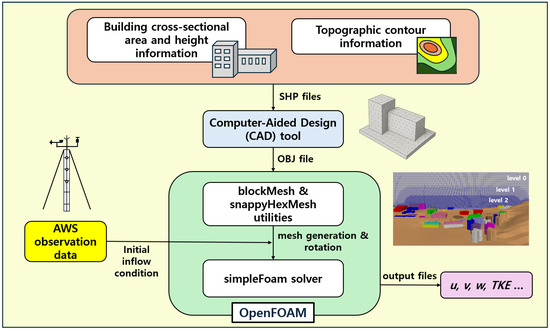
Figure 1.
Flowchart showing the microscale urban airflow modeling system.
2.2. Simulation Domain and Configuration
The developed system was applied to the area surrounding the University of Seoul campus (located in Dongdaemun-gu, Seoul, South Korea) to simulate microscale airflow. The AWS station of KMA in Dongdaemun (Station 408) is located on the rooftop of the Changgong Hall building within the University of Seoul campus. The modeling domain was centered at this station, and the observed meteorological data were used for the analysis. In order to utilize upwind meteorological data as inflow boundary conditions, a search within a 6 km radius of the modeling domain identified four AWS stations. Accordingly, four simulation cases were designed using data from nearby AWS stations located northwest (Seongbuk), northeast (Nowon), southwest (Seongdong), and east (Jungnang) of Station 408 (Figure 2a). Cases were selected based on instances in which winds blew from each AWS station toward Station 408, under neutral atmospheric stability conditions. Neutral atmospheric stability was determined using ASOS (synoptic weather station) data by selecting periods without precipitation, with total cloud cover above 8.5 okta, wind speeds exceeding 2 m s−1, and solar radiation below 0.2 MJ m−2, which correspond to Pasquill stability class D [33]. Each case was named according to the inflow wind direction and the AWS station number used for each case. The date, wind speed, and wind direction for each case are summarized in Table 1. For example, the NW414 case refers to a simulation conducted using boundary conditions based on a representative event with northwesterly (NW) inflow, selected using data from the Seongbuk station (Station 414, Figure 2a). A logarithmic inflow wind profile was generated from the 10 m wind speed data of each corresponding AWS station and applied at the inflow boundary of the domain.
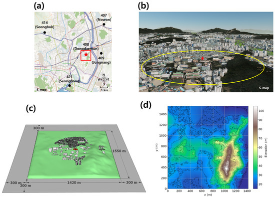
Figure 2.
(a) Map showing locations of the five Automatic Weather System (AWS) stations, (b) rendered image displaying building heights and terrain elevation across the campus and its surroundings, (c) CFD domain with building layouts and terrain, and (d) terrain elevation contour map within the domain. The red star indicates the location of Station 408, and the red box in (a) indicates the modeling domain. The yellow circle in (b) represents a 500 m radius centered at the station.

Table 1.
Case name, AWS station name, date, and time of the selected event, inflow wind speed at 10 m (WS10m), and inflow wind direction (WD) used as boundary conditions for the four cases.
The modeling domain was configured to include Changgong Hall, located near the center of the domain, along with Baebong Mountain and the surrounding terrain. A 3D geometry was constructed using terrain elevation data and building information. Small structures that may cause numerical instability during simulation (e.g., container boxes) were excluded, and buildings within a 500 m radius, such as campus facilities, high-rise apartment complexes, and commercial and residential buildings, were incorporated (Figure 2b). To ensure proper boundary treatment, buffer zones of 300 m were added in both the x and y directions, resulting in domain sizes of 2020 m (x), 2150 m (y), and 300 m (z) (Figure 2c). The terrain elevation of the modeling domain is shown in Figure 2d, and Baebong Mountain within the domain rises slightly above 100 m. The blockMesh utility was used to generate a base mesh with a resolution of 10 m. To resolve airflow near buildings more accurately, finer meshes were generated using the snappyHexMesh utility, with a resolution of 5 m within 100 m of building surfaces and at least 2.5 m within 50 m. A grid sensitivity test with a minimum grid size of 1.25 m was conducted, confirming that the selected grid resolution is adequate to capture the essential flow features around buildings and to analyze urban wind patterns. Each of the four simulation cases was conducted for 9000 iterations, and the airflow at the final iteration was analyzed. The number of iterations was determined through a convergence test showing that the residuals stabilized and the solution reached a quasi-steady state.
3. Results and Discussion
3.1. Model Validation
The OpenFOAM model was validated by comparing simulation results with wind-tunnel data from the CEDVAL A1-1 case at the University of Hamburg, Hamburg, Germany, focusing on key flow features around a single cuboid obstacle (Figure 3) [34]. The spatial scales were normalized by building height, and velocities were normalized by the 100 m mean inflow velocity to enable comparison between the two datasets. The OpenFOAM model slightly overestimates flow separation along the lateral sides compared with the wind-tunnel results. It also shows differences in the rear recirculation region, with the center displaced outward from the centerline ( = 0; Figure 3a,b). Because of the limited grid resolution near the ground surface, the reattachment length could not be calculated directly. Instead, we identified the location at which the wake streamlines diverge in the lowest grid cell near the ground surface. The estimated locations are = 2.44 in the OpenFOAM model and = 1.56 in the wind-tunnel experiment, indicating a notable difference. The discrepancy is consistent with the findings of Wang et al. (2023) [35] and Vardoulakis et al. (2011) [36], who reported that RANS models tend to overestimate the extent of the wake and have difficulty in accurately reproducing the weak-wind region behind buildings compared with wind-tunnel experiments. Despite such discrepancies, the OpenFOAM model reasonably reproduced the key flow features observed in the wind-tunnel experiments, including the corner vortex near the lower upwind side, flow separation at the top and lateral corners, and the wake and internal recirculation on the downwind side of the obstacle, indicating that overall, the model is capable of capturing the flow around the obstacle.
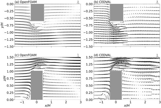
Figure 3.
Wind vector fields of the OpenFOAM simulations (a,c) and CEDVAL wind-tunnel experiments (b,d). Normalized wind vectors are shown on the (a,b) x–y plane at = 0.28 and the (c,d) x–z plane at = 0.
3.2. Urban Airflow Analysis with the Developed Modeling System
We simulated four cases and compared the simulated wind speed and direction at the location of Station 408 (53 m above sea level) with the observed data from Station 408 (Figure 4). The simulated airflow generally follows the inflow wind direction with slight deceleration, with wind directions deviating within 8° and wind speeds within 0.79 m s−1. The simulation results show good consistency with the observations, including those at Station 408, with wind directions deviating within 37.4°. However, the simulated wind directions tend to be biased counterclockwise relative to the measured directions, and wind speed deviations of up to 1.12 m s−1 are observed depending on the case. The discrepancies may be due to simplified terrain and building data and incomplete representation of meteorological conditions (e.g., atmospheric stability). In this study, a logarithmic inflow wind profile was constructed and applied based on AWS station data located more than 2.2 km away from Station 408. However, terrain effects between the AWS stations and the modeling domain were not considered, which may have introduced significant errors. Overall, the simulation results are in good agreement with the observations.
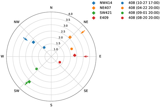
Figure 4.
Polar plot of wind direction and wind speed, where the distance from the center represents wind speed (m s−1). Arrow markers indicate the inflow conditions for the four cases. Circle markers indicate the observation data from Station 408, and diamond markers represent the corresponding OpenFOAM simulation results at the same location.
Figure 5 presents the fields of horizontal wind vector and speed at z = 53 m for the four cases over the entire domain (0 m < x < 1420 m, 0 m < y < 1550 m), excluding the buffer region. In all four cases, the simulations were stably integrated for up to 9000 iterations without numerical instability. Mass conservation was maintained without divergence caused by mismatched boundary conditions or abnormal pressure distributions at the domain boundaries. The overall flow appears similar to the inflow, and the structure and characteristics of the wake flow field are appropriately reproduced. In the downwind areas of campus buildings and high-rise apartments, pronounced wakes with a sharp decrease in wind speed are observed. A wake extending several hundred meters also forms on the leeside of Baebong Mountain. In the NE407 and E409 cases, these two wake patterns overlap, resulting in a significant deceleration in the flow. These wakes also affect the wind at Station 408, with the NE407 and E409 cases, which are characterized by strong wake formation, showing a particularly large discrepancy from the inflow (Figure 4).
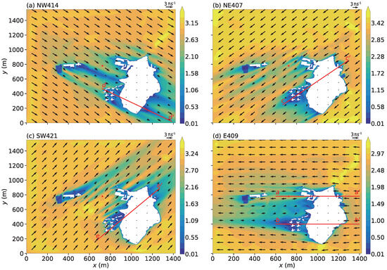
Figure 5.
Fields of wind vector and speed on the x–y plane at z = 53 m for the (a) NW414, (b) NE407, (c) SW421, and (d) E409 cases. Color shading indicates wind speed (m s−1) and the red star marks the location of Station 408. To simplify visual interpretation, wind vectors are displayed at 100 m intervals, and the buffer region has been omitted from the figure.
In the E409 case, where the wake effect caused by the mountain is most pronounced, the wind pattern around Baebong Mountain was closely examined (Figure 6). At a height of 53 m, flow separation occurs at the southern and northern edges of Baebong Mountain, resulting in a downstream wake of comparable size. On the leeward side of Baebong Mountain (x = 730−900 m, y = 300−400 m), near the high-rise apartment buildings, the flow pattern within the wake becomes more complex because of the additional recirculation generated by the buildings. In areas where wakes overlap due to multiple distinct topographic features, the flow becomes weak and highly complex. Although Station 408 is influenced by the wake, local channeling near the station leads to wind speeds exceeding 2 m s−1, which is a notable feature. At a height of 80 m, a wake comparable in scale to Baebong Mountain also forms and develops in three branches, consistent with the mountainous terrain. Although the wake can still be detected at 130 m, which is above the height of Baebong Mountain, it becomes less discernible with increasing altitude.
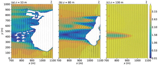
Figure 6.
Fields of wind vector on the x–y plane (700 m < x < 1100 m, 0 m < y < 1000 m) for the E409 case at the (a) z = 53 m, (b) z = 80 m, (c) z = 130 m. Color shading represents wind speed (m s−1) and the red star indicates the location of Station 408. To clarify visual analysis, wind vectors are displayed at 20 m intervals.
To investigate the effects of Baebong Mountain and high-rise apartments on wind patterns, wind vectors and wind speed were analyzed on the x–z plane intersecting Baebong Mountain for the four cases (Figure 7 and Figure 8). In all cases, updrafts develop along the windward slope of Baebong Mountain, which can be attributed to the high Froude number under neutral atmospheric stability conditions [37,38]. In the E409 case, two cross-sections were analyzed—one at y = 780 m, intersecting Station 408, and another at y = 400 m, near the summit of Baebong Mountain and traversing a high-rise apartment complex (see Figure 5 for the locations) (Figure 7a,b). Whereas a distinct wake does not develop at the y = 780 m cross-section, at y = 400 m, the wake is well developed on the leeward side, extending vertically up to approximately 130 m. Recirculation appears within the wake, with the center of circulation reaching the summit elevation of Baebong Mountain. In the NE407 case, although high-rise apartment buildings are also located on the leeward side of Baebong Mountain, the wake does not extend significantly above the mountain height as observed in the E409 case (Figure 7c). This may be because the northeasterly wind does not directly interact with the wake formed behind the apartment complex.
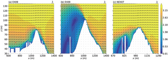
Figure 7.
Fields of wind vector on the x–z plane for the E409 case along segments (a) aa′ and (b) bb′, and for the NE407 case along segment (c) cc′. The locations of the segments are indicated in Figure 5. Color shading represents wind speed (m s−1), and the red star marks the location of the wind measurement instrument installed at Station 408. To make visual analysis clearer, wind vectors are displayed at 20 m intervals.
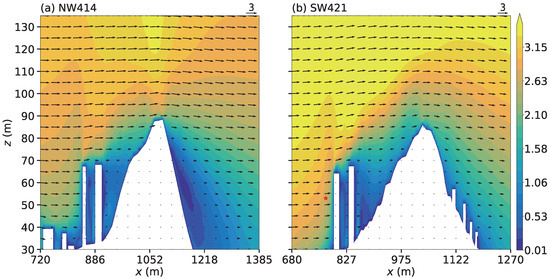
Figure 8.
Fields of wind vector on the x–z plane for the NW414 case along segments (a) dd′, and for the SW421 case along segment (b) ee′. The locations of the segments are indicated in Figure 5. Color shading represents wind speed (m s−1) and the red star marks the location of the wind measurement instrument installed at Station 408. To make visual analysis clearer, wind vectors are displayed at 20 m intervals.
As shown in Figure 7b, a strong wake develops on the leeward side of Baebong Mountain under specific conditions and locations, even under neutral atmospheric stability and without significant thermal forcing. This appears to be influenced by the presence of a high-rise apartment complex. To verify this interpretation, an additional cross-sectional analysis was conducted for the NW414 and SW421 cases, where high-rise buildings are absent on the leeward side. In the NW414 case, wake and recirculation also develop, but their vertical extent is substantially smaller than that in the E409 case, likely due to the absence of high-rise buildings on the leeward side (Figure 8a). In the SW421 case, the wake was also reduced in extent, and inner recirculation was entirely disturbed by the hillside buildings (Figure 8b).
We closely investigated the airflow around the Changgong Hall, where Station 408 is located. Figure 9 shows the horizontal wind vectors and vertical wind speed at a height of 37 m, corresponding to the mid-level of Changgong Hall, for the four cases. All four cases exhibit complex horizontal and vertical flow structures within a densely built-up area, where the influence of adjacent buildings overlapped. Updrafts and downdrafts occur on the leeward side of buildings with respect to the inflow, indicating the presence of wakes and internal recirculations. Horizontal flow separation occurs at the windward faces of the buildings as the incoming wind impinges on their surfaces. The intensity and pattern of separation vary depending on the inflow strength, prevailing wind direction, and surrounding building configuration. In addition, in the westerly cases, strong updrafts are observed on the leeward side of Changgong Hall, whereas in easterly cases, pronounced downdrafts are observed on the windward side. This is likely due to the influence of slope winds blowing along the inclined surface of Baebong Mountain, leading to highly complex flow patterns around buildings located on slopes.
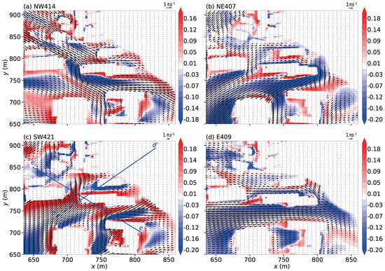
Figure 9.
Fields of wind vector on the x–y plane (635 m < x < 860 m, 650 m < y < 910 m, z = 37 m) for the (a) NW414, (b) NE407, (c) SW421, and (d) E409 cases. Color shading represents w velocity (m s−1) and the red star denotes the location of Station 408. The segments dd′, and ee′ indicate the locations of the cross-sections in panels a, and b of Figure 10, respectively. To improve clarity of the flow field, wind vectors are displayed at 5 m intervals.
To further investigate the complex flow around Changgong Hall, we analyzed velocity fields along planes both parallel and perpendicular to the inflow in the SW421 case (Figure 10). In the inflow-parallel plane, flow separation is observed in front of the buildings, and a vortex appears between Changgong Hall and the building to the north as a cross-sectional manifestation of helical flow (Figure 10a). In the inflow-perpendicular plane, a vortex associated with a helical flow is also observed near the building located south of Changgong Hall. The flow separations and wakes around the buildings are connected to the channeling flow, forming a complex helical flow pattern (Figure 10b). The inflow direction is not perfectly aligned with the building layout, making it difficult to clearly identify the flow regime. Nonetheless, distinct vortical flows are observed in areas with closely spaced buildings, where insufficient ventilation may lead to localized air pollution [11,39]. In addition, in the inflow-parallel plane, an updraft develops along the slope of Baebong Mountain, complicating local flow patterns and potentially influencing pollutant dispersion locally. In particular, within the confined space formed by the slope and surrounding buildings, changes in atmospheric stability are expected to significantly alter both the flow and dispersion patterns, highlighting the need for further investigation [40].
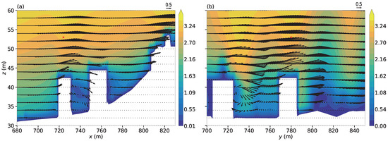
Figure 10.
Fields of wind vector on the (a) x–z plane along segment dd′, and (b) y–z plane along segment ee′ for the SW421 case. The locations of these segments are indicated in Figure 9. Color shading indicates wind speed (m s−1) and the red star denotes the location of the wind measurement instrument installed at Station 408. To improve clarity of the flow field, wind vectors are displayed at 2 m intervals.
Figure 11 illustrates the helical flow structure in more detail between Changgong Hall and the adjacent northern building in the SW421 case. The helical flows arise from the interaction between the approaching southwesterly wind and the street-canyon space between the two buildings. Flow separation at the northwestern windward corner of Changgong Hall generates rotating vortices, which are tilted by vertical wind shear and evolve into helical flows.
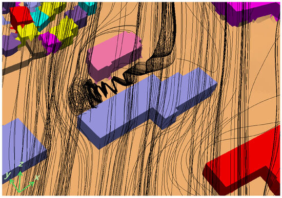
Figure 11.
Visualization of helical flows between Changgong Hall and the adjacent northern building in the SW421 case, rendered using ParaView.
4. Summary and Conclusions
In this study, we developed a modeling system for simulating microscale urban airflow that incorporates both urban buildings and terrain features. The system generates 3D geometry files using publicly available building morphography data and terrain elevation information, followed by the creation of a hexahedral-dominant unstructured mesh that conforms to the urban surface geometry. The open-source CFD model OpenFOAM was employed, with the simpleFoam solver, and inflow boundary conditions were applied based on observational data from nearby AWS stations, also publicly available. To demonstrate its applicability, the modeling system was applied to the urban area surrounding the University of Seoul in South Korea.
Microscale airflow simulations were performed for four cases (NW414, NE407, SW421, and E409), each representing inflow conditions from the four AWS stations surrounding the University of Seoul. The simulation results were compared with observational data from Station 408. Although there were some discrepancies, such as a counterclockwise bias in the simulated wind direction relative to observations, the overall agreement in both wind direction and speed was reasonable. Flow separation and wakes were observed behind buildings and on the leeward side of Baebong Mountain. In the NE407 and E409 cases, where high-rise buildings are located on the leeward side of the mountain, overlapping wake effects from the complex terrain and tall structures led to greater reductions in wind speed. In particular, the E409 case exhibited strong recirculation within the wake, with the recirculation center reaching an elevation similar to the summit of Baebong Mountain, likely due to the influence of high-rise buildings located within the wake. This intensified flow pattern was not observed in the NW414 case, where the wake region did not contain tall buildings. Building-scale flow separation and wakes were also reproduced around Station 408, located near Changgong Hall. Notably, helical flows developed between buildings and manifested as vortex structures within the street canyon between Changgong Hall and neighboring buildings. The results confirm that the developed airflow modeling system effectively captures the influence of both urban structures and terrain features, successfully simulating microscale urban airflow.
This study focused on neutral atmospheric stability without thermal forcing. At the current stage, thermally driven flows, such as mountain-valley winds and urban heat island circulations, cannot be simulated due to the absence of thermal processes. In the next stage, we plan to incorporate heat transfer processes by using a Boussinesq solver (e.g., buoyantBoussinesqPimpleFoam). Another limitation was the use of simplified inflow boundary conditions. To develop a concise modeling framework, these were derived from nearby AWS observations. However, discrepancies may occur because of the substantial distance between the AWS stations and the modeling domain, where intervening terrain effects may be underrepresented and atmospheric profiles can change over such distances. To overcome the limitations related to atmospheric stability and observational distance, mesoscale meteorological models such as the Weather Research and Forecasting (WRF) model could be considered to provide boundary condition data for simulations. Although vegetation (e.g., trees) can significantly influence urban airflow through increased surface roughness and drag [41], this study does not account for vegetation effects in the modeling framework. Future extensions of the system may include vegetation effects to improve accuracy in realistic urban settings. In addition, while the current system focuses on steady-state flow simulations, we recognize that temporal effects play an important role in complex urban environments. To address this limitation, development of a URANS-based modeling framework is planned as the next step to more accurately capture unsteady flow features. Despite such limitations, this study is notable because it establishes a system capable of accurately simulating and analyzing microscale urban airflow using openly available terrain, building, and meteorological data. With further development, the system could be applied to urban wind comfort, microclimate, and pollutant dispersion modeling, thereby contributing to climate adaptation and air quality improvement.
Author Contributions
Investigation, validation, visualization, formal analysis, writing—original draft preparation, writing—review and editing, H.-B.A.; conceptualization, methodology, supervision, project administration, funding acquisition S.-B.P. All authors have read and agreed to the published version of the manuscript.
Funding
This work was supported by the 2021 Research Fund of the University of Seoul for Seung-Bu Park. Also, this work was supported by the Korea Meteorological Administration Research and Development Program under Grant RS-2024-00404042 for Hyo-Been An.
Institutional Review Board Statement
Not applicable.
Informed Consent Statement
Not applicable.
Data Availability Statement
The data presented in this study are available upon request from the corresponding author.
Acknowledgments
The authors are grateful to three anonymous reviewers for providing valuable comments on this study.
Conflicts of Interest
The authors declare no conflicts of interest.
References
- Fernando, H. Fluid dynamics of urban atmospheres in complex terrain. Annu. Rev. Fluid Mech. 2010, 42, 365–389. [Google Scholar] [CrossRef]
- Oke, T.R. Street design and urban canopy layer climate. Energy Build. 1988, 11, 103–113. [Google Scholar] [CrossRef]
- Toparlar, Y.; Blocken, B.; Maiheu, B.; van Heijst, G.J.F. A review on the CFD analysis of urban microclimate. Renew. Sust. Energ. 2017, 80, 1613–1640. [Google Scholar] [CrossRef]
- Britter, R.E.; Hanna, S.R. Flow and dispersion in urban areas. Annu. Rev. Fluid Mech. 2003, 35, 469–496. [Google Scholar] [CrossRef]
- Baklanov, A.; Grimmond, C.S.B.; Carlson, D.; Terblanche, D.; Tang, X.; Bouchet, V.; Lee, B.; Langendijk, G.; Kolli, R.K.; Hovsepyan, A. From urban meteorology, climate and environment research to integrated city services. Urban Clim. 2018, 23, 330–341. [Google Scholar] [CrossRef]
- Santiago, J.; Martilli, A. A dynamic urban canopy parameterization for mesoscale models based on computational fluid dynamics Reynolds-averaged Navier–Stokes microscale simulations. Bound.-Layer Meteorol. 2010, 137, 417–439. [Google Scholar] [CrossRef]
- Qiu, Y.; He, Y.; Li, M.; Zhu, X. A Generalization of Building Clusters in an Urban Wind Field Simulated by CFD. Atmosphere 2023, 15, 9. [Google Scholar] [CrossRef]
- Tominaga, Y.; Stathopoulos, T. CFD simulation of near-field pollutant dispersion in the urban environment: A review of current modeling techniques. Atmos. Environ. 2013, 79, 716–730. [Google Scholar] [CrossRef]
- Li, Z.; Han, B.; Chu, Y.; Shi, Y.; Huang, N.; Shi, T. Evaluating the Impact of Road Layout Patterns on Pedestrian-Level Ventilation Using Computational Fluid Dynamics (CFD). Atmosphere 2025, 16, 123. [Google Scholar] [CrossRef]
- Pantusheva, M.; Mitkov, R.; Hristov, P.O.; Petrova-Antonova, D. Air pollution dispersion modelling in urban environment using CFD: A systematic review. Atmosphere 2022, 13, 1640. [Google Scholar] [CrossRef]
- An, H.B.; Park, S.B. Assessing urban ventilation using large-eddy simulations. Build. Environ. 2024, 263, 111899. [Google Scholar] [CrossRef]
- Zhang, C.; Yu, Z.; Zhu, Q.; Shi, H.; Yu, Z.; Xu, X. Air-Permeable Building Envelopes for Building Ventilation and Heat Recovery: Research Progress and Future Perspectives. Buildings 2023, 14, 42. [Google Scholar] [CrossRef]
- Kang, G.; Kim, J.J.; Choi, W. Computational fluid dynamics simulation of tree effects on pedestrian wind comfort in an urban area. Sustain. Cities Soc. 2020, 56, 102086. [Google Scholar] [CrossRef]
- Ioannidis, G.; Li, C.; Tremper, P.; Riedel, T.; Ntziachristos, L. Application of CFD modelling for pollutant dispersion at an urban traffic hotspot. Atmosphere 2024, 15, 113. [Google Scholar] [CrossRef]
- Park, S.B.; Baik, J.J.; Han, B.S. Large-eddy simulation of turbulent flow in a densely built-up urban area. Environ. Fluid Mech. 2015, 15, 235–250. [Google Scholar] [CrossRef]
- Li, S.; Sun, X.; Zhang, S.; Zhao, S.; Zhang, R. A study on microscale wind simulations with a coupled WRF–CFD model in the Chongli mountain region of Hebei Province, China. Atmosphere 2019, 10, 731. [Google Scholar] [CrossRef]
- Baik, J.J.; Park, S.B.; Kim, J.J. Urban flow and dispersion simulation using a CFD model coupled to a mesoscale model. J. Appl. Meteorol. Climatol. 2009, 48, 1667–1681. [Google Scholar] [CrossRef]
- Liu, J.; Niu, J. CFD simulation of the wind environment around an isolated high-rise building: An evaluation of SRANS, LES and DES models. Build. Environ. 2016, 96, 91–106. [Google Scholar] [CrossRef]
- Park, S.B.; Baik, J.J.; Raasch, S.; Letzel, M.O. A large-eddy simulation study of thermal effects on turbulent flow and dispersion in and above a street canyon. J. Appl. Meteorol. Climatol. 2012, 51, 829–841. [Google Scholar] [CrossRef]
- Kavian Nezhad, M.R.; Lange, C.F.; Fleck, B.A. Performance evaluation of the RANS models in predicting the pollutant concentration field within a compact urban setting: Effects of the source location and turbulent Schmidt number. Atmosphere 2022, 13, 1013. [Google Scholar] [CrossRef]
- Liu, S.; Pan, W.; Zhao, X.; Zhang, H.; Cheng, X.; Long, Z.; Chen, Q. Influence of surrounding buildings on wind flow around a building predicted by CFD simulations. Build. Environ. 2018, 140, 1–10. [Google Scholar] [CrossRef]
- Versteeg, H.K.; Malalasekera, W. An Introduction to Computational Fluid Dynamics the Finite Volume Method; Pearson Education India: Noida, India, 1995. [Google Scholar]
- Launder, B.E.; Spalding, D.B. The numerical computation of turbulent flows. In Numerical Prediction of Flow, Heat Transfer, Turbulence and Combustion; Elsevier: Amsterdam, The Netherlands, 1983; pp. 96–116. [Google Scholar] [CrossRef]
- Greenshields, C.; Weller, H. Notes on Computational Fluid Dynamics: General Principles; CFD Direct Ltd.: Reading, UK, 2022. [Google Scholar]
- OpenCFD. OpenFOAM Documentation: atmNutUWallFunction 2023. Available online: https://doc.openfoam.com/2306/tools/processing/boundary-conditions/rtm/derived/atmospheric/atmNutUWallFunction/ (accessed on 2 June 2025).
- Latif, H.; Hultmark, G.; Rahnama, S.; Maccarini, A.; Afshari, A. Performance evaluation of active chilled beam systems for office buildings—A literature review. Sustain. Energy Technol. Assess. 2022, 52, 101999. [Google Scholar] [CrossRef]
- Tominaga, Y.; Mochida, A.; Yoshie, R.; Kataoka, H.; Nozu, T.; Yoshikawa, M.; Shirasawa, T. AIJ guidelines for practical applications of CFD to pedestrian wind environment around buildings. J. Wind Eng. Ind. Aerodyn. 2008, 96, 1749–1761. [Google Scholar] [CrossRef]
- Patankar, S. Numerical Heat Transfer and Fluid Flow; CRC Press: Boca Raton, FL, USA, 1980. [Google Scholar] [CrossRef]
- Weller, H.G.; Tabor, G.; Jasak, H.; Fureby, C. A tensorial approach to computational continuum mechanics using object-oriented techniques. Comput. Phys. 1998, 12, 620–631. [Google Scholar] [CrossRef]
- National Geographic Information Institute. National Spatial Information Portal. 2025. Available online: https://map.ngii.go.kr/mn/mainPage.do (accessed on 2 June 2025).
- Mohammadian, A.; Kheirkhah Gildeh, H.; Yan, X. An introduction to OpenFOAM. In Numerical Simulation of Effluent Discharges; Taylor & Francis: Oxfordshire, UK, 2023. [Google Scholar] [CrossRef]
- Korea Meteorological Administration. Open MET Data Portal. 2025. Available online: https://data.kma.go.kr/cmmn/main.do (accessed on 2 June 2025).
- Pasquill, F. Atmospheric dispersion of pollution. Q. J. R. Meteorol. Soc. 1971, 97, 369–395. [Google Scholar] [CrossRef]
- Environmental Wind Tunnel Laboratory, University of Hamburg. CEDVAL A1-1: Experimental Data for CFD Validation—Isolated Building. 2001. Available online: https://www.mi.uni-hamburg.de/en/arbeitsgruppen/windkanallabor/data-sets.html (accessed on 2 June 2025).
- Wang, Y.; Li, J.; Liu, W.; Zhang, S.; Dong, J. Prediction of urban airflow fields around isolated high-rise buildings using data-driven non-linear correction models. Build. Environ. 2023, 246, 110894. [Google Scholar] [CrossRef]
- Vardoulakis, S.; Dimitrova, R.; Richards, K.; Hamlyn, D.; Camilleri, G.; Weeks, M.; Sini, J.F.; Britter, R.; Borrego, C.; Schatzmann, M.; et al. Numerical model inter-comparison for wind flow and turbulence around single-block buildings. Environ. Model. Assess. 2011, 16, 169–181. [Google Scholar] [CrossRef]
- Cheng, L.W.; Yu, C.K.; Chen, S.P. Identifying mechanisms of tropical cyclone generated orographic precipitation with Doppler radar and rain gauge observations. Npj Clim. Atmos. Sci. 2025, 8, 35. [Google Scholar] [CrossRef]
- Wise, A.S.; Neher, J.M.; Arthur, R.S.; Mirocha, J.D.; Lundquist, J.K.; Chow, F.K. Meso-to micro-scale modeling of atmospheric stability effects on wind turbine wake behavior in complex terrain. Wind Energy Sci. 2021, 2021, 1–36. [Google Scholar] [CrossRef]
- Oke, T.R.; Mills, G.; Christen, A.; Voogt, J.A. Urban Climates; Cambridge University Press: Cambridge, UK, 2017. [Google Scholar]
- Finardi, S.; Morselli, M.; Jeannet, P.; Szepesi, D.; Vergeiner, I.; Deligiannis, P.; Lagouvardos, K.; Planinsek, A.; Borrel, L.; Fekete, K.; et al. Wind Flow Models over Complex Terrain for Dispersion Calculations; Report of Working Group 4, COST Action 710; Office for Official Publications of the European Communities: Luxembourg, 1997. [Google Scholar]
- Ricci, A.; Guasco, M.; Caboni, F.; Orlanno, M.; Giachetta, A.; Repetto, M. Impact of surrounding environments and vegetation on wind comfort assessment of a new tower with vertical green park. Build. Environ. 2022, 207, 108409. [Google Scholar] [CrossRef]
Disclaimer/Publisher’s Note: The statements, opinions and data contained in all publications are solely those of the individual author(s) and contributor(s) and not of MDPI and/or the editor(s). MDPI and/or the editor(s) disclaim responsibility for any injury to people or property resulting from any ideas, methods, instructions or products referred to in the content. |
© 2025 by the authors. Licensee MDPI, Basel, Switzerland. This article is an open access article distributed under the terms and conditions of the Creative Commons Attribution (CC BY) license (https://creativecommons.org/licenses/by/4.0/).