Quantifying the Influence of Sea Surface Temperature Anomalies on the Atmosphere and Precipitation in the Southwestern Atlantic Ocean and Southeastern South America

Abstract

Oceanic mesoscale activity influences the atmosphere in the southwestern and southern sectors of the Atlantic Ocean. However, the influence of high latitudes, specifically sea ice, on mid-latitudes and a better understanding of mesoscale ocean–atmosphere thermodynamic interactions still require further study. To quantify the effects of oceanic mesoscale activity during the periods of maximum and minimum Antarctic sea ice extent (September 2019 and February 2020), numerical experiments were conducted using a coupled regional model and an online two-dimensional spatial filter to remove high-frequency sea surface temperature (SST) oscillations. The largest SST anomalies were observed in the Brazil–Malvinas Confluence and along oceanic fronts in September, with maximum SST anomalies reaching 4.23 °C and −3.71 °C. In February, the anomalies were 2.18 °C and −3.06 °C. The influence of oceanic mesoscale activity was evident in surface atmospheric variables, with larger anomalies also observed in September. This influence led to changes in the vertical structure of the atmosphere, affecting the development of the marine atmospheric boundary layer (MABL) and influencing the free atmosphere above the MABL. Modulations in precipitation patterns were observed, not only in oceanic regions, but also in adjacent continental areas. This research provides a novel perspective on ocean–atmosphere thermodynamic coupling, highlighting the mesoscale role and importance of its representation in the study region.

1. Introduction

The influence of polar regions on the oceans, weather, and climate at mid-latitudes remains uncertain, particularly regarding how sea ice, which is highly susceptible to climatic changes, affects these areas. It is hypothesized that the meridional temperature gradient of the oceans, influenced by periods of maximum and minimum sea ice extent, may impact mesoscale oceanic features, which could, in turn, modulate both the ocean and the atmosphere, locally and remotely.

The influence of mesoscale oceanic structures on the atmosphere has been studied in the literature due to the modulation they exert on the surface atmosphere, the marine atmospheric boundary layer (MABL), and even above it, in the free atmosphere [1,2,3,4,5,6,7,8,9]. Mesoscale oceanic structures can be defined as oceanographic fronts, meanders, and eddies with horizontal scales of ≈100 km and temporal scales from days to three months [7,8,9,10,11,12]. In these ocean–atmosphere interaction studies, it has been observed that positive (negative) anomalies in sea surface temperature (SST), caused by mesoscale oceanic structures, generally lead to positive (negative) anomalies in air temperature, near-surface wind, and sensible (Hs) and latent Hl heat fluxes. An opposite response is expected in sea level pressure (SLP), where negative (positive) SLP anomalies have been associated with positive (negative) SST anomalies.

Regarding the vertical structure of the atmosphere, studies have shown [8,13,14] that increased heat fluxes from the ocean to the atmosphere over positive SST anomalies lead to increased turbulence within the MABL. In such cases, an unstable MABL and a decrease in vertical wind shear are observed, leading to an increase in surface wind and a deepening of this layer. However, an opposite response is observed over negative SST anomalies. The modulations caused by SST anomalies in the surface and vertical structure of the atmosphere also influence precipitation [3,5,15]. Regarding this, [3] demonstrated how positive (negative) SST anomalies associated with oceanic eddies lead to wind anomalies that result in the convergence (divergence) of surface winds and vertical motions, thereby intensifying (decreasing) precipitation.

The Southwestern Atlantic Ocean (SWA) is characterized by significant oceanic mesoscale activity related to the confluence of the Brazil Current (BC) and the Malvinas Current (MC), a region known as the Brazil–Malvinas Confluence (BMC), and by the presence of the subtropical front (STF) and the subantarctic front (SAF) (Figure 1) [7,11,16,17]. Eddies and meanders form year-round in these regions with intense thermal gradients, where warmer and saltier waters confluence with colder and fresher waters, mainly due to baroclinic instability [7,12,18]. However, oceanic mesoscale activity is not limited to mid-latitudes, such as the SWA; it can also occur in other regions, like the Southern Ocean, where the presence of mesoscale eddies influences precipitation [3]. Additionally, horizontal SST gradients in high latitudes over the polar front (PF) have seasonal variations, showing smaller temperature gradients during summer [17,19]. Climatologically, maximum sea ice extent is observed in this region in September, at the end of austral winter, while minimum extent occurs in February, at the end of austral summer [20].

Given the recognized importance of oceanic mesoscale activity in influencing the atmosphere, this study enhances our understanding of the thermodynamic relationship between these two environments. Besides that, coupled ocean–atmosphere models have been crucial in understanding this thermodynamic coupling in several regions of the global ocean [2,5,21,22,23,24,25,26]. In this study, a regional coupled model is used for the first time to quantify the impact of oceanic mesoscale activity on the atmosphere in the southwestern and southern sectors of the Atlantic Ocean and its relationship with the maximum and minimum sea ice extent around the Antarctic Peninsula. A two-dimensional spatial filter is implemented to remove the high-frequency SST associated with the oceanic mesoscale. Furthermore, the influence of oceanic mesoscale activity on precipitation in southeastern South America was also investigated.

The study is organized as follows: Section 2 outlines the numerical experiments, defines the two-dimensional spatial filter used, and describes the methodology for analyzing ocean–atmosphere interaction processes. Section 3 discusses the impact of oceanic mesoscale activity (I) on the lower atmosphere, (II) on the modulation of the vertical structure of the atmosphere, and (III) on precipitation. Section 4 presents the conclusions and a schematic model (cartoon) representing the main findings of the study.

2. Methodology

This section describes the regional coupled numerical modeling system and the numerical experiments conducted. It also provides an overview of the two-dimensional spatial filter used within the modeling system to remove SST anomalies associated with oceanic mesoscale activity. Finally, this section concludes by describing the methodology for analyzing ocean–atmosphere interaction processes.

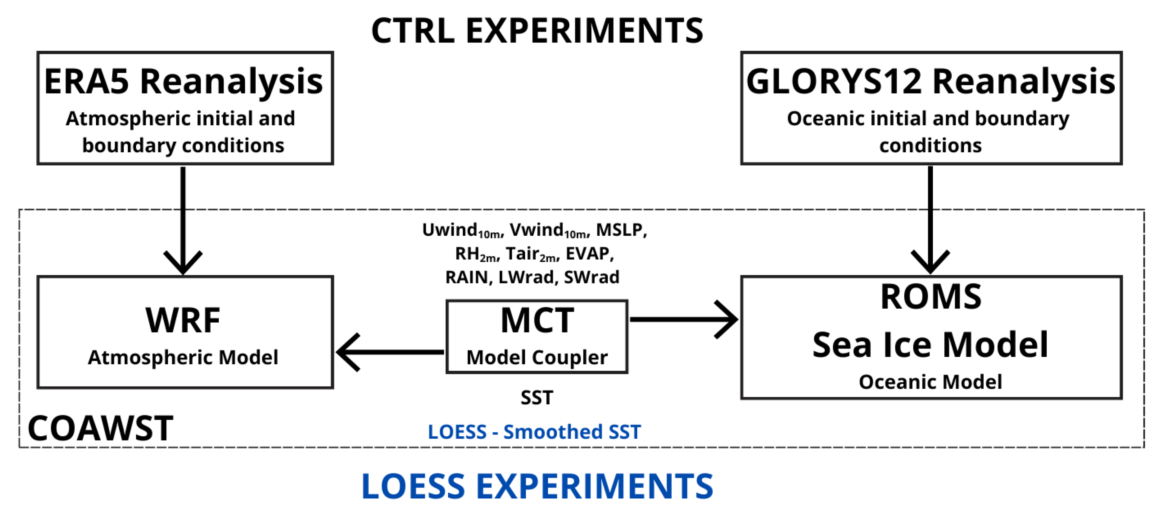
2.1. Numerical Experiments Description

The numerical experiments were conducted using the Coupled Ocean Atmosphere Wave Sediment Transport (COAWST v3.4) Modeling System [27]. From this version of the regional COAWST modeling system, the atmospheric model Weather Research and Forecasting Model (WRF v4.0.3) [28], the oceanic model Regional Ocean Modeling System (ROMS svn 934) [29,30,31], and the Sea Ice Model [32] were activated. Data exchange between the WRF and ROMS models was performed using the Model Coupling Toolkit (MCT v2.6.0) [33,34].

The domain used in numerical experiments extends between the latitudes of 19° S and 66° S and the longitudes of 85° W and 27° W (Figure 1). To generate atmospheric initial and boundary conditions, data from the ERA5 reanalysis [35] was utilized. Variables from this reanalysis were used every 3 h from both pressure levels (with 37 levels covering from 1000 hPa to 1 hPa) and single levels. This data is provided on a regular latitude–longitude grid with a resolution of 1/4°. For oceanic initial and boundary conditions, data from the global eddy-resolving physical ocean and sea ice GLORYS12 reanalysis [36] was employed. This dataset has a daily temporal resolution and is also provided on a regular longitude–latitude grid with a spatial resolution of 1/12°. The data includes 50 vertical levels, ranging from 0 to approximately 5500 m in depth.

The horizontal resolution of the grids was 12 km for both the WRF and ROMS models. In the WRF model, 45 vertical levels and a time step of 20 s were defined. The same set of physical parameterizations used by [37] was employed for resolving sub-grid processes. In the ROMS model, 30 vertical levels were used, with a baroclinic time step of 90 s and 40 barotropic sub-steps. The physical parameterizations used in the ROMS model were also employed in the previous study of [37] in the SWA region. Additionally, the model outputs are generated every 3 h. In coupled modeling, the models exchange variables with one another (Figure A1). In our configuration of the coupled model, this variable exchange occurs every 900 s [26].

The numerical experiments were performed for a month of maximum sea ice extent and a month of minimum sea ice extent to ensure that the effects of oceanic mesoscale activity were not masked over several years. The simulation period for the month of maximum sea ice extent was 31 days, beginning on 31 August 2019, and concluding on 1 October 2019, with an emphasis on analyzing the variables in September 2019. For the month of minimum sea ice extent, the simulation period was 30 days, starting on 31 January 2020 and ending on 1 March 2020; in this case, the variable analysis focused on February 2020.

2.2. Nudging Areas and Verifying Simulations

In the first numerical experiments, biases were observed in the ocean variables, particularly at the western boundary of the domain, associated with the Antarctic Circumpolar Current (ACC), which was driving the transport of warmer waters to higher latitudes, causing sea ice melt. To reduce these biases, an area near the boundaries was defined where nudging coefficients ($1/\psi$, with $\psi$ representing the time scale for the nudging coefficient) were calculated, following [38]. The nudging areas for the western, northern, and eastern boundaries were defined for 15 grid points from the boundary point (representing ≈ 1.6°), while the southern nudging area was defined for 50 grid points (≈5.4°), as indicated by the thick black line in Figure 1. A larger southern nudging area was defined to reduce the biases in the southwest of the domain, considering that the main goal is to study the influence of oceanic mesoscale activity, which was mainly observed over oceanic fronts at latitudes lower than the southern nudging area. The nudging coefficients vary from a time scale of five days at the external boundary points, decreasing linearly to zero (i.e., no nudging) at the inner boundary of the nudging areas.

In the nudging areas, the model’s equations were approximated to external data by adding the nudging term, represented in Equation (1), on the right side of the model’s prognostic equations [39,40]:

$$-{\displaystyle \frac{1}{\psi }}(\varphi -{\varphi }^{ext})$$

(1)

In this term, ${\varphi }^{ext}$ represents the external data. The potential temperature, salinity, and the u and v components of the currents from the GLORYS12 reanalysis were used as external climate data. In this study, all numerical experiments consider this nudging area when solving the ROMS model equations.

Outside the nudging area, the model runs freely without correction, allowing for the study of ocean–atmosphere interaction processes. To verify the simulations, comparisons were made between the simulated SST, sea ice concentration, precipitation, and data from satellites and reanalysis (Figure A2, Figure A3, Figure A4). The simulated SST and those obtained from the Multi-scale Ultra-high Resolution (MUR) [41] for the study periods are shown in Figure A2a, Figure A2b, Figure A2d, and Figure A2e, respectively. Comparing these fields, it is observed that the model accurately represents the main oceanic features observed in the MUR data. To calculate the bias between the two datasets, a horizontal interpolation of the MUR data onto the ROMS grid was first performed. The largest biases in September are observed in regions with larger SST gradients (Figure A2c), particularly in the SWA region, which is characterized by significant variability and oceanic mesoscale activity. In February, a predominance of positive biases is observed (Figure A2f), highlighting the SWA region and the area around the Antarctic Peninsula. The presence of warmer waters near the Weddell Sea is evident when comparing the 0 °C isotherms in Figure A2d,e. However, outside of these areas with higher variability, it is observed that the biases are not significant and that the study’s goals can be achieved. Therefore, it can be concluded that the model adequately represented the SST.

The comparison of sea ice concentration is shown in Figure A3. The observed sea ice concentration is provided by the EUMETSAT Ocean and Sea Ice Satellite Application Facility (OSI SAF) High-Latitude Processing Center [42]. Overall, the model adequately represents the areas with sea ice. For the month of maximum sea ice extent (Figure A3a,b), particularly between longitudes 80° W and 30° W, the model shows a larger sea ice extent than the EUMETSAT data. This is also related to the negative SST biases observed in the marginal ice zone during September (Figure A2c). In February, the model represents a smaller sea ice extent in the same area around the Antarctic Peninsula, where positive SST biases are observed (Figure A2f and Figure A3c,d).

In analyzing simulated precipitation, data from the ERA5 reanalysis, which was also used to generate the initial and boundary atmospheric conditions (Section 2.1), as well as data from the Global Satellite Mapping of Precipitation (GSMaP) [43], were utilized (Figure A4). Due to the spatial coverage observed in the GSMaP data during the study periods, a smaller domain than the model grid was used for comparing the precipitation (19° S–55.5° S and 85° W–27° W). For the simulated data from both periods, it is observed that regions with larger precipitation correspond to areas where the maximum precipitation is estimated in the GSMaP data and represented in the ERA5 data. In September, in the SWA, between latitudes 37° S and 50° S, regions with approximately 6 mm of precipitation that seem to respond to the mesoscale oceanic structures present in the area are highlighted (Figure A4a). This precipitation is not as clearly estimated in the GSMaP data, but it is observed in the ERA5 reanalysis data (Figure A4b,c). The evaluated fields confirmed that the simulations satisfactorily represent the main oceanic and atmospheric characteristics during the study periods. The simulations used in this section are the CTRL experiments discussed in the sections below.

2.3. Description and Definition of the LOESS Filter

The Locally Weighted Smoothing (LOESS) filter was used to quantify the influence of oceanic mesoscale activity on the atmosphere [2,44,45]. This filter was implemented in the MCT, the coupler of the COAWST system, to remove high-frequency oscillations from the SST associated with oceanic mesoscale activity. This was performed at each coupling step when the ROMS supplied the SST to the WRF. Thus, two types of coupled experiments were conducted: CTRL experiments, where the ocean mesoscale was fully present, and LOESS experiments, where a smoothed SST was supplied to the WRF. The differences between these two types of experiments (CTRL-LOESS) enabled the identification of atmospheric variable anomalies induced by oceanic mesoscale activity. This filter has been used in previous studies to analyze ocean–atmosphere interaction processes [2,21,22,46,47,48,49].

LOESS is a two-dimensional horizontal spatial filter (latitude and longitude) that uses a tri-cubic weighting function:

$$w\left(x\right)={(1-|x|}^3{)}^3,\left|x\right|<1$$

(2)

where x represents the distance between the subset points and the desired point. This function assigns a larger weight to points nearer to the desired point and a smaller weight to points farther away. The maximum SST anomalies, defined as the difference between the SST of the CTRL experiment and the SST of the LOESS experiment, depend on the smoothing parameter (half-span), which is related to the half of the filtering window in the zonal and meridional directions. Therefore, five sensitivity tests were conducted for the period of maximum sea ice extent (September 2019) to define the half-span that more accurately represents the ocean mesoscale in the study area. The SST anomalies derived from the five sensitivity tests were represented in mean probability distributions, which aided in defining the most appropriate half-span [48].

The probability distributions of the mean SST anomalies for the five sensitivity tests are shown in Figure 2. In these sensitivity tests, half-spans of 3°× 3°, 4°× 4°, 5°× 5°, 6°× 6°, and 7°× 7° for latitude and longitude were used, respectively. In the probability distributions, it was observed that the maximum mean SST anomalies increase with each sensitivity test as the half-span increases. Meanwhile, the differences between the probability distributions gradually decreased until minimal variation was observed between experiments four (6°× 6°) and five (7°× 7°). Therefore, it was concluded that a half-span of 6°× 6° accurately represents the ocean mesoscale in the study area.

With the LOESS half-span and simulation periods defined, four simulations were conducted to examine the influence of oceanic mesoscale activity on the atmosphere (

Table 1. Summary of the four numerical experiments conducted to investigate the influence of oceanic mesoscale activity on the atmosphere. The first column defines the names of the four numerical experiments, the second column illustrates the simulation period for each, and the third column indicates which experiment had the LOESS filter activated and which did not.

Numerical Experiment	Analyzed Period	LOESS Filter
CTRLSIMAX	September 2019	No
LOESSIMAX	September 2019	Yes
CTRLSIMIN	February 2020	No
LOESSIMIN	February 2020	Yes

). (I) CTRLSIMAX (without LOESS) and (II) LOESSIMAX (with LOESS) were performed for the maximum Antarctic sea ice extent (September 2019). (III) CTRLSIMIN (without LOESS) and (IV) LOESSIMIN (with LOESS) were carried out for the minimum Antarctic sea ice extent (February 2020). Figure A1 illustrates a flow chart of the numerical experiments representing the steps followed in the simulations, the data and tools used, and the main difference between the CTRL and LOESS runs.

2.4. Ocean–Atmosphere Interaction Processes Analysis

In analyzing the influence of ocean mesoscale on atmospheric variables, anomalies were defined as the mean of the difference between the respective variable from the CTRL and LOESS experiments at each model output time step, following Equation (3):

$$anomaly={\displaystyle \frac{1}{n}}\sum _{i=1}^n(a_{CTRL}-a_{LOESS})$$

(3)

where a represents the desired variable and n the number of model output time steps. The surface atmospheric variable anomalies analyzed were 2 m air temperature (Tair), SLP, 10 m wind, and net surface energy balance (Qnet). Qnet was calculated as the sum of the shortwave radiation balance (Sw), longwave radiation balance (Sw), Hs, and Hl, following Equation (4) [50]:

$$Qnet=Sw+Lw+Hs+Hl$$

(4)

Meridional atmospheric profiles were used to investigate how oceanic mesoscale activity modulates the vertical structure of the atmosphere. The profiles were created between latitudes 34° S and 60° S at 52° W, along the SST anomalies observed in the BMC and crossing the PF. The atmospheric variable anomalies analyzed in the vertical profiles included equivalent potential temperature (${\theta }_e$), the MABL top height, and the meridional and vertical components of wind. ${\theta }_e$ is also an indicator of the moisture present in the atmosphere. The correlation between the MABL top height anomalies and SST anomalies for the study periods was also calculated for the latitudes of the meridional profile.

The influence of oceanic mesoscale activity on precipitation was investigated by analyzing the anomalies of total accumulated precipitation during the study periods and the standard deviation of daily precipitation anomalies. The analysis focused on the region with the largest SST anomalies in SWA and southeastern South America, particularly southern Brazil and Uruguay, as indicated by the purple rectangles in Figure 1. For these subregions, we calculated the percentage contributions of oceanic mesoscale activity to both the daily mean precipitation and the total accumulated precipitation during the study months.

3. Results and Discussion

3.1. Influence of Oceanic Mesoscale on the Lower Atmosphere

This section examines how surface atmospheric variables respond to oceanic mesoscale activity. The quantification of the anomalies in these variables caused by SST anomalies is presented, emphasizing the differences between the month of maximum (September 2019) and minimum (February 2020) sea ice extent.

The mean SST from the CTRLSIMAX and LOESSIMAX experiments for September 2019 is shown in Figure 3a,b. The SST anomaly derived from the previous fields is shown in Figure 3c. The largest anomalies are observed in the BMC region and along the SAF in the SWA (Figure 3c). In these regions, the anomalies have a meridional and zonal orientation, respectively. This distribution of anomalies follows the ocean current circulation in the area [51] and coincides with regions of larger eddy kinetic energy [18]. The maximum positive and negative anomalies were 4.23 °C and −3.71 °C, respectively. Significant anomaly values (≈±2 °C) are also observed in the regions of the STF in the SWA and the PF along the ACC.

The mean SST for February 2020 shows larger values in the northern part of the study region and a southward shift of the BC compared to the characteristics observed in September (Figure 3a,d). The characteristics seen in the SST for February represent typical austral summer conditions, when warmer waters are transported farther south by the BC, and a minimum Antarctic sea ice extent is observed [20,52]. Overall, the distribution of SST anomalies for February shows little variation in the SWA region, with the largest values observed in the BMC region and along the SAF (Figure 3f). However, a decrease in the magnitude of these anomalies is verified, particularly for positive SST anomalies. The maximum positive and negative anomalies for this month are 2.18 °C and −3.06 °C. The magnitude of SST anomalies along the ACC and at latitudes above 50° S has also decreased compared to those observed in September (Figure 3c,f). The decrease in the magnitudes of SST anomalies in the ACC region can be related to the decrease in the meridional SST gradient observed along the PF during the austral summer [19].

The modulation of Tair by oceanic mesoscale activity is shown in Figure 4a,b. The largest Tair anomalies are observed in September, particularly in the SWA region and along the ACC, where the largest SST anomalies occur (Figure 3c and Figure 4a). Positive anomalies of up to 1.09 °C and negative anomalies of up to −1.92 °C were observed in Tair, indicating the impact of oceanic mesoscale activity on the overlying atmosphere. In February, the relationship between Tair and SST anomalies is also evident (Figure 3f and Figure 4b). The decrease in the magnitudes of Tair anomalies this month (maximum anomalies of up to 0.99 °C and −1.52  °C) is associated with the decrease in the magnitudes of SST anomalies.

In the SLP anomaly for September, a predominance of negative values is observed, induced by positive SST anomalies (Figure 4c). This can also be verified in the maximum SLP anomalies, which are −0.39 hPa and 0.08 hPa, respectively. The predominance of negative SLP anomalies during the period of maximum sea ice extent can also be related to the circulation of the South Atlantic Subtropical High (SASH). The SASH is located further north in the CTRLSIMAX experiment compared to its mean position in the LOESSIMAX experiment, resulting in negative anomalies to the south of its area of influence. In February, the more southern position of the SASH, combined with the influence of oceanic mesoscale activity and synoptic atmospheric transients, resulted in an interesting tripole pattern in SLP anomalies in the SWA (Figure 4d). The maximum SLP anomalies for February are −0.37 hPa and 0.28 hPa, respectively. The magnitudes of the SLP anomalies are comparable to the ranges observed in surface pressure anomalies (±0.25 hPa) induced by mesoscale SST anomalies (±4 °C) in the Southern Ocean Indian sector region [2].

The relationship between positive (negative) SST anomalies and positive (negative) 10 m wind anomalies can be verified in Figure 3c,f and Figure 4e,f. This relationship indicates that the 10 m wind speed increases (decreases) over warmer (colder) waters, consistent with studies conducted in oceanic fronts and ocean mesoscale eddies [1,8,11,12,14,50]. The maximum 10 m wind speed anomalies for September are 0.93 m s⁻¹ and −1.35 m s⁻¹, respectively, while for February, they are 0.95 m s⁻¹ and −1.21 m s⁻¹, respectively.

Qnet anomalies for September and February are shown in Figure 4g,h. The distributions of anomalies for this variable demonstrate the impact of mesoscale oceanic structures on the surface energy balance. This influence on Qnet occurs mainly due to differences in properties between the ocean and atmosphere, such as temperature and moisture, combined with the effect of mesoscale oceanic structures on the wind, which directly modulates turbulent heat fluxes (Hl and Hs).

The largest Qnet anomalies are observed in September, particularly in the SWA region (Figure 4g,h). The maximum Qnet anomalies are 178.88 W m⁻² and −115.03 W m⁻² in September and 95.71 W m⁻² and −98.78 W m⁻² in February, respectively. The Qnet anomalies observed in September are comparable to those identified by [8] using in situ data sampled in the SWA in October 2019. Among the components of Qnet, turbulent heat fluxes are the main contributors to the observed anomalies. The maximum anomalies for September are 133.08 W m⁻² and −85.58 W m⁻² for Hl and 68.33 W m⁻² and −46.48 W m⁻² for Hs. For February, the maximum anomalies are 75.65 W m⁻² and −86.04 W m⁻² for Hl and 27.63 W m⁻² and −21.59 W m⁻² for Hs, respectively.

Overall, the analyzed surface atmospheric variables showed larger anomalies during the month of maximum sea ice extent (at the end of the austral winter) than during the month of minimum sea ice extent (in the austral summer). This relates to the larger SST anomalies observed during the period of maximum sea ice extent. The anomaly values for SST, Tair, and the sensible and latent heat fluxes are comparable to those presented by [5] in the Kuroshio–Oyashio Confluence region. The authors used numerical experiments to include eddies with 3 °C positive SST anomalies. These anomalies increased the near-surface air temperature by 1–1.5 °C, resulting in a 180 W m⁻² increase in heat flux (Hl + Hs).

3.2. Modulation of the Vertical Structure of the Atmosphere

The SST anomalies associated with mesoscale oceanic structures could modulate not only surface atmospheric variables but also the vertical structure of the atmosphere, as demonstrated in this section. Figure 5a,c show how the oceanic mesoscale indeed modulates the vertical development of the MABL during both studied periods. Positive (negative) anomalies of the MABL top height are observed in regions where warm (cold) eddies and meanders are present, indicating a greater (lesser) development of this layer. The maximum positive (negative) anomalies of the MABL top height in September reach values of up to 142 m (−223 m), respectively, while in February, anomalies of up to 91 m (−199 m) are observed.

The clear similarity among the patterns observed in the anomalies of SST, Tair, 10 m wind, Qnet, and the MABL top height evidences the effect of the vertical mixing mechanism [13]. This mechanism explains the MABL’s response to a horizontal ocean temperature gradient through modifications in the surface flux. Given that the positive (negative) anomalies of surface flux over positive (negative) SST anomalies lead to an increase (decrease) in turbulence in the MABL, deepening (shallowing) this layer, the increase (decrease) in turbulence in the MABL also increases (decreases) downward momentum transport, which decreases (increases) vertical wind shear and increases (decreases) surface winds. The following variables, represented in the meridional vertical profiles (the thick black line in Figure 5a,c), illustrate the anomalies in the MABL.

The ${\theta }_e$ anomalies, represented by blue and red tones, and the MABL top height from the CTRL experiments, depicted by the black line, are shown in Figure 6a,b for the meridional profiles in September and February, respectively. In the meridional profiles, a relationship is observed between the MABL top height, positive (negative) ${\theta }_e$ anomalies, and positive (negative) SST anomalies (Figure 6a,b,g,h). There is a strong correlation between the MABL top height anomalies and SST anomalies for the meridional profiles, with values of 0.83 in September and 0.76 in February, respectively (Figure 5b,d). The largest magnitudes of ${\theta }_e$ anomalies occur at latitudes north of 49° S (Figure 6a,b), coinciding with a greater development of the MABL, which reached heights of up to 834 m in September (Figure 6a). At latitudes south of 49° S, where the smallest ${\theta }_e$ anomalies are verified, no significant changes in the MABL top height are observed when comparing the periods of maximum and minimum sea ice extent. The mean MABL top height for this region is 404 m in September and 384 m in February (Figure 6a,b).

Meridional wind anomalies indicate an acceleration (deceleration) of meridional winds in the near-surface atmosphere above warmer (colder) waters (Figure 6c,d,g,h). For this variable, unlike the ${\theta }_e$ anomalies that occur just above the SST anomalies, the meridional wind anomalies show a slight shift to the south. This shift in wind response has been described in studies analyzing the atmospheric modulation induced by oceanic mesoscale eddies. Previous studies have shown that wind convergence shifts to the edge of the eddies [5,8].

Mesoscale oceanic structures also impact the vertical wind component, as seen in Figure 6e,f. In September, particularly at latitudes north of 49° S, a direct relationship between vertical wind speed anomalies and SST anomalies can be verified. At 42° S and 44° S, where the largest positive and negative anomalies of vertical wind occur (Figure 6e), ascending and descending movements are observed in the CTRLSIMAX experiment, respectively. These movements are intensified by the oceanic mesoscale, as evidenced by vertical wind anomalies. The unclear response of vertical wind during the month of minimum sea ice extent can be associated with the smaller amplitude of SST anomalies observed in February (Figure 6e–h).

Yet another remarkable result of this study is the verification of oceanic mesoscale influences on the free atmosphere above the MABL. This is evident in the vertical profiles, where the ${\theta }_e$ anomalies propagate above the MABL top height (Figure 6a,b). This propagation through the MABL to the free atmosphere can be related to the wind dynamics within the MABL. An increase (decrease) in surface wind was observed over positive (negative) SST anomalies, which may indicate a convergence (divergence) of the surface wind, along with ascending (descending) movements, as observed in the meridional profiles. This vertical wind transport may lead to the vertical advection of temperature influenced by the SST anomalies that penetrate into the free atmosphere above the larger SST anomalies. This result agrees with the influence on the free atmosphere, as previously suggested by [8], who analyzed ERA5 data for a warm oceanic eddy.

The results presented here regarding the modulation of the vertical structure of the atmosphere by SST anomalies emphasize that the relationship between these two environments is more pronounced during the period of maximum sea ice extent when the largest SST anomalies occur. This relationship is more evident at latitudes north of 49° S, reaching into the free atmosphere. The influence of a warm oceanic eddy on the free atmosphere in the SWA was verified in a prior study using vertical wind data from the ERA5 reanalysis [8], as previously mentioned. At latitudes south of 49° S, atmospheric variable anomalies did not show significant differences between the periods of maximum and minimum Antarctic sea ice extent.

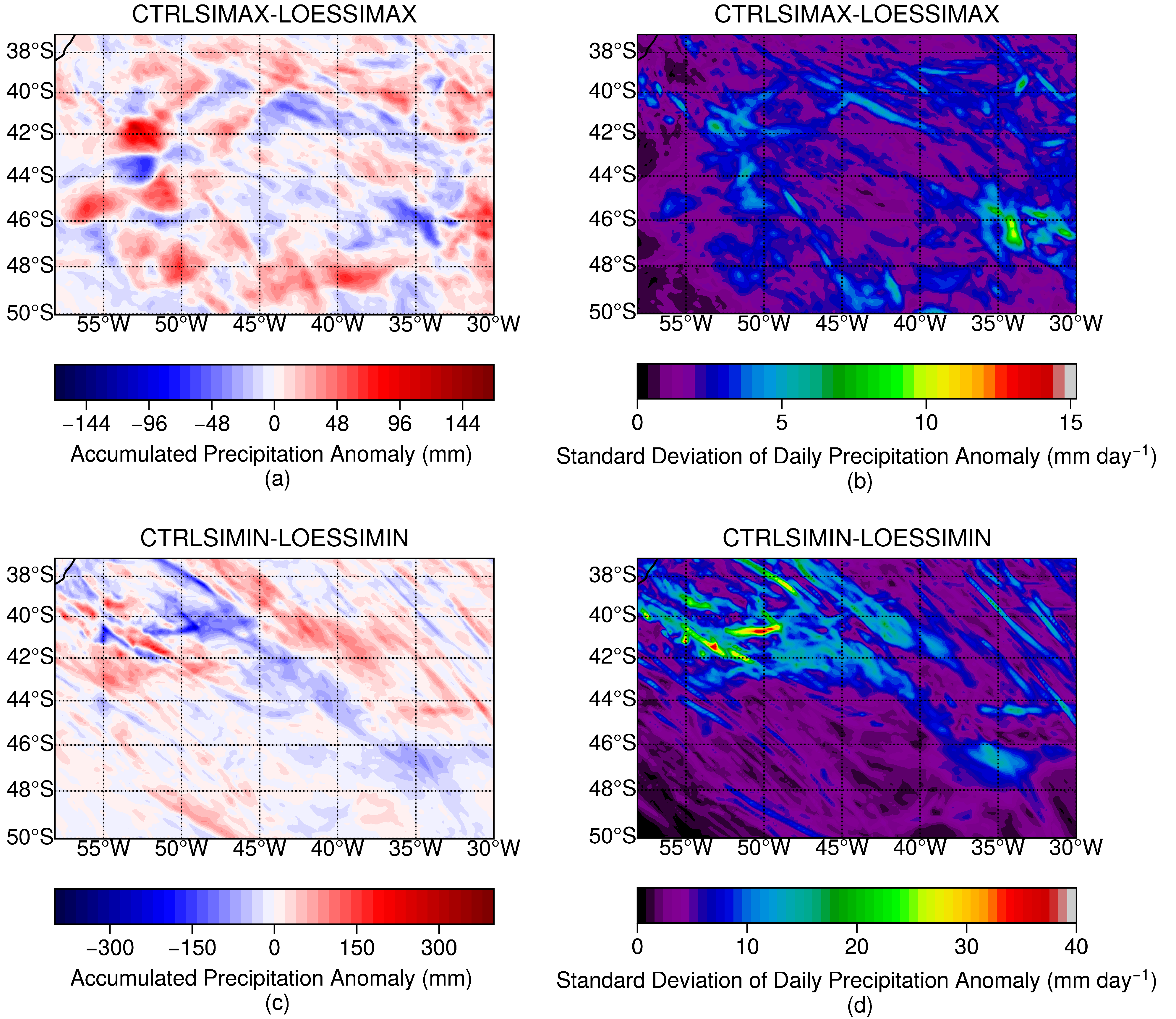
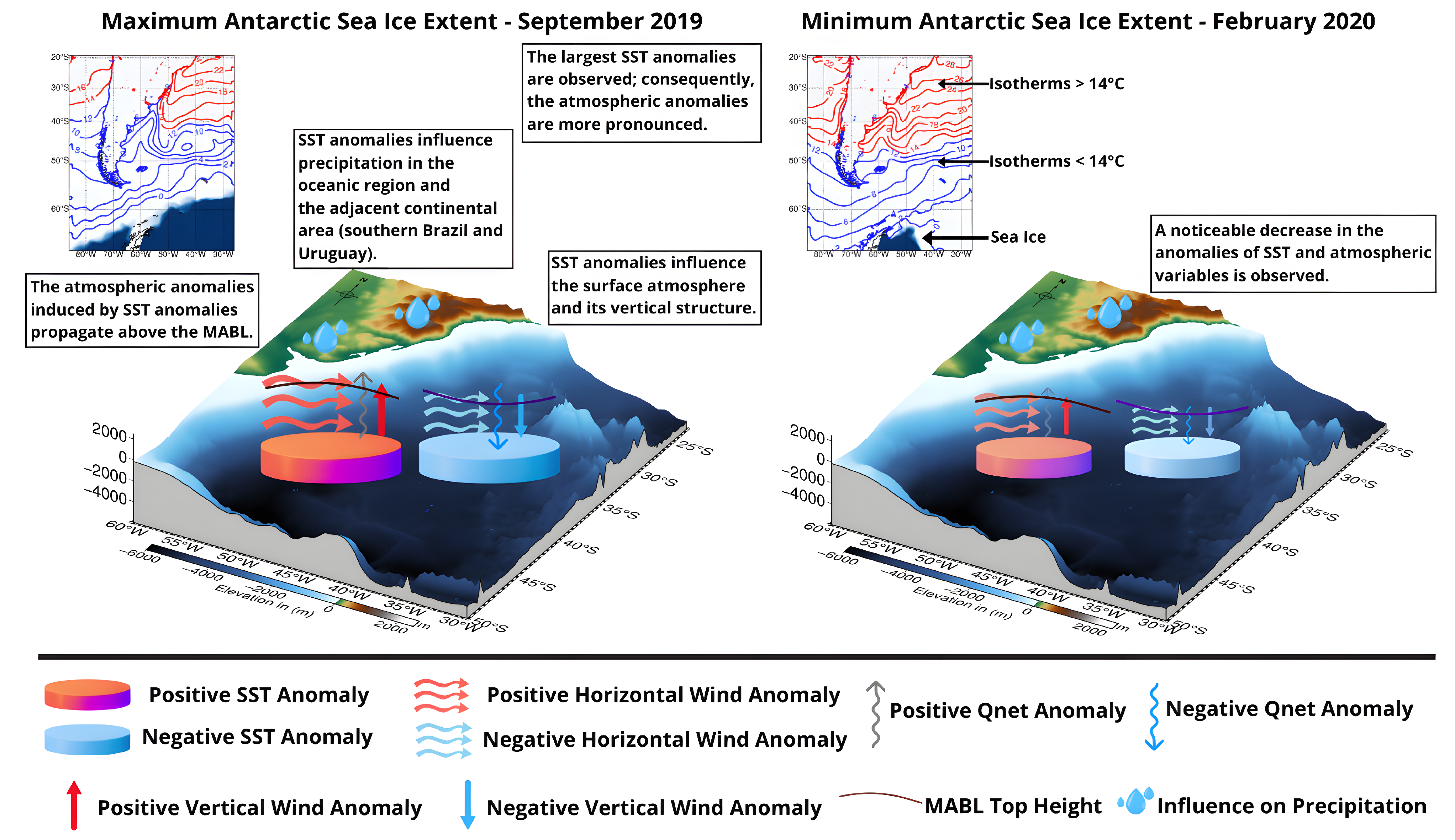
3.3. Influence of Oceanic Mesoscale on Precipitation

This section shows the influence of oceanic mesoscale activity on precipitation. The results indicate that oceanic mesoscale activity not only modifies precipitation locally in the region where they are present but also influences the distribution of precipitation in the continental region northwest of the largest oceanic mesoscale activity.

Figure 7a,b show the total accumulated precipitation for September from the CTRLSIMAX and LOESSIMAX experiments, respectively. Comparing these two fields demonstrates the influence of oceanic mesoscale activity on precipitation. The black rectangle in the ocean highlights the subregion where there is larger mesoscale activity modulating precipitation. For this subregion, Figure 8a shows the accumulated precipitation anomaly, while Figure 8b presents the standard deviation of daily precipitation anomalies. The accumulated precipitation anomalies indicate that positive (negative) anomalies occur where positive (negative) SST anomalies are present (Figure 3c and Figure 8a). The maximum anomalies observed in precipitation for the subregion are 123 mm and −73 mm, respectively. Positive SST anomalies contributed to an increase of up to 50% in total accumulated precipitation in some areas, while negative SST anomalies contributed, in some cases, to inhibiting the precipitation. The standard deviation of daily precipitation anomalies indicates the areas where these anomalies were more pronounced in relation to their mean value (Figure 8b). Regarding this modulation, ref. [3] analyzed the precipitation response associated with warm and cold eddies in the Southern Hemisphere (south of 30° S) and suggested that processes induced by SST anomalies likely remain restricted to the MABL. This contrasts with the results presented here, which also indicate an impact on the free atmosphere. This difference from the study by [3] may be related to the SST anomalies observed here (maximum anomalies of 4.23 °C and −3.71  °C), which are larger than those reported in their study (anomalies of ≈0.5#xA0;°C and −0.5 °C).

The total accumulated precipitation for February from the CTRLSIMIN and LOESSIMIN experiments is presented in Figure 7c,d. Changes in the distribution of total accumulated precipitation can be verified by comparing the experiments with and without oceanic mesoscale activity. The accumulated precipitation anomalies for February in the oceanic subregion show a northwest–southeast orientation associated with changes in precipitation distribution influenced by the oceanic mesoscale (Figure 8c). The maximum anomalies related to changes in precipitation distribution are approximately 192 mm and −287 mm, respectively. A similar orientation is observed in the standard deviation of daily precipitation anomalies (Figure 8d).

For this oceanic subregion, the time series of daily mean precipitation, the standard deviation of daily precipitation, and the accumulated daily mean precipitation for the CTRL and LOESS experiments are analyzed. No significant differences are observed between the CTRL and LOESS experiments when comparing the daily mean precipitation time series. However, when calculating the contributions of mesoscale oceanic structures to daily mean precipitation for this subregion ((CTRL-LOESS)%), predominantly positive values between ≈1 and 18% are observed in September. This contributes to an increase in the accumulated daily mean precipitation driven by the presence of the oceanic mesoscale in the CTRLSIMAX experiment. In this case, the contribution of mesoscale oceanic structures to the accumulated daily mean precipitation is 2.59%. In February, the opposite situation is observed; the CTRLSIMIN experiment shows smaller accumulated daily mean precipitation than the LOESSIMIN experiment. In this case, the contribution of mesoscale oceanic structures to daily mean precipitation presents both positive and negative values, with variations ranging from ≈0.02% to 18% and from −23% to −0.02%, respectively. This results in a negative contribution of mesoscale oceanic structures to the accumulated daily mean precipitation, which is ≈−1.65%. This is the only case analyzed in which the presence of mesoscale oceanic structures leads to a decrease in mean precipitation in the studied subregions.

In the continental region northwest of the analyzed oceanic subregion, differences in simulated precipitation are also observed between the CTRL and LOESS experiments (the black rectangle over the continent in Figure 7). Accumulated precipitation anomalies were calculated for September and February in this area, which includes southern Brazil and Uruguay (Figure 9a,c). The maximum anomalies observed in September (February) reach values of up to approximately 90 mm (280 mm) for positive anomalies and −72 mm (−266 mm) for negative anomalies, respectively. Figure 9b,d show the areas where daily precipitation anomalies are larger relative to their mean value. The presence of precipitation anomalies in this continental subregion emphasizes the influence that oceanic mesoscale activity can have, not only on the overlying atmosphere but also on the synoptic systems that produce precipitation in adjacent continental areas.

The time series of the mean and standard deviation of daily precipitation and the accumulated daily mean precipitation for the continental subregion are also analyzed for the study months. The daily mean precipitation in September shows little difference between the CTRLSIMAX and LOESSIMAX experiments. However, the accumulated daily mean precipitation is slightly larger for the CTRLSIMAX experiment. The contributions of mesoscale oceanic structures to daily mean precipitation show a predominance of positive values, ranging from 0.1% to 24%. This results in a contribution of 1.86% to the accumulated daily mean precipitation. In February, a more pronounced difference was observed between the CTRLSIMIN and LOESSIMIN experiments, particularly due to the positive contributions from oceanic mesoscale activity, with values between 0.15 and 63%. This leads to a larger positive contribution of 4.81% to the accumulated daily mean precipitation.

In summary, the accumulated precipitation anomalies reflect both local and remote responses associated with SST anomalies. In the SWA region, a direct relationship can be observed between positive (negative) precipitation anomalies and positive (negative) SST anomalies during the period of maximum sea ice extent. It is emphasized that during this period, the largest SST anomalies were observed. However, the CTRLSIMIN and LOESSIMIN experiments also show changes in the distribution of total accumulated precipitation in the SWA during the period of minimum sea ice extent. In the adjacent continental region, a positive contribution of oceanic mesoscale activity to accumulated daily mean precipitation is observed. This contribution in the continental region, distant from the ocean, can be attributed to the influence of SST anomalies on atmospheric circulation. The pattern observed in the SLP anomalies illustrates the differences between the experiments with and without SST anomalies, showing that the synoptic systems can also be influenced by the presence of mesoscale oceanic structures. These results demonstrate how the adequate representation of mesoscale oceanic structures in coupled numerical models can provide more accurate results in weather and climate simulations.

4. Conclusions

This study provides a novel perspective on oceanic mesoscale activity in the SWA and its influence on the atmosphere, both locally and in southeastern South America. Studies on this oceanic region, from the perspective of ocean–atmosphere interaction, are still very scarce in the literature. This challenge of studying the effects of the mesoscale ocean–atmosphere thermodynamic interactions is extremely motivating, and the good results obtained are very gratifying. There are still several scientific points that need to be further explored; however, we have taken a good first step in this direction.

Numerical experiments using a coupled regional model were conducted to investigate and quantify the impact of oceanic mesoscale activity on the atmosphere by employing a two-dimensional spatial filter (LOESS) and examining its relationship with Antarctic sea ice extent. The experiments revealed that the atmospheric responses were associated with the presence of oceanic mesoscale activity. The anomalies of the surface atmospheric variables responded to ocean mesoscale activity, as described in the literature. However, they were more pronounced during the period of maximum Antarctic sea ice extent when the largest SST anomalies were also observed. The anomaly values presented here corroborate those obtained for other oceanic regions but are unprecedented for this region of the global ocean.

Oceanic mesoscale activity also modulated the vertical structure of the atmosphere. The largest anomalies of the variables represented in meridional vertical profiles were observed in regions with the largest SST anomalies. These responses propagated into the free atmosphere above the MABL. The filter used in this study also enabled the analysis of how oceanic mesoscale activity influenced precipitation. It was observed that this influence was not limited to the oceanic region but also extended to the adjacent continental area. The results show that the accumulated daily mean precipitation was larger in southern Brazil and Uruguay when mesoscale structures were present in the simulations. Figure 10 shows a schematic representation summarizing the main findings of the study.

This study demonstrates the importance of oceanic mesoscale activity in atmospheric modulation and how it can influence not only the local overlying atmosphere but also the climate of South America. This leads us to conclude how crucial the representation of mesoscale oceanic structures is in the numerical experiments. The inadequate representation of ocean–atmosphere thermodynamic processes at this scale can lead to systematic errors and increased uncertainties in weather and climate studies and forecasts. A future study will investigate the impact of oceanic mesoscale activity on synoptic systems that influence South America and, consequently, Brazil.

References

1. Pezzi, L.; Souza, R.; Dourado, M.; Garcia, C.; Mata, M.; Silva-Dias, M. Ocean–atmosphere in situ observations at the Brazil–Malvinas Confluence region. Geophys. Res. Lett. 2005, 32, L24603. [Google Scholar] [CrossRef]
2. O’Neill, L.W.; Esbensen, S.K.; Thum, N.; Samelson, R.M.; Chelton, D.B. Dynamical analysis of the boundary layer and surface wind responses to mesoscale SST perturbations. J. Clim. 2010, 23, 559–581. [Google Scholar] [CrossRef]
3. Frenger, I.; Gruber, N.; Knutti, R.; Münnich, M. Imprint of Southern Ocean eddies on winds, clouds and rainfall. Nat. Geosci. 2013, 6, 608–612. [Google Scholar] [CrossRef]
4. Villas Bôas, A.B.; Sato, O.T.; Chaigneau, A.; Castelão, G.P. The signature of mesoscale eddies on the air-sea turbulent heat fluxes in the South Atlantic Ocean. Geophys. Res. Lett. 2015, 42, 1856–1862. [Google Scholar] [CrossRef]
5. Sugimoto, S.; Aono, K.; Fukui, S. Local atmospheric response to warm mesoscale ocean eddies in the Kuroshio–Oyashio confluence region. Sci. Rep. 2017, 7, 11871. [Google Scholar] [CrossRef] [PubMed]
6. Desbiolles, F.; Meroni, A.N.; Renault, L.; Pasquero, C. Environmental Control of Wind Response to Sea Surface Temperature Patterns in Reanalysis Dataset. J. Clim. 2023, 36, 3881–3893. [Google Scholar] [CrossRef]
7. Leyba, I.M.; Saraceno, M.; Solman, S.A. Air-sea heat fluxes associated to mesoscale eddies in the southwestern Atlantic Ocean and their dependence on different regional conditions. Clim. Dyn. 2017, 49, 2491–2501. [Google Scholar] [CrossRef]
8. Pezzi, L.P.; Souza, R.B.; Santini, M.F.; Miller, A.J.; Carvalho, J.T.; Parise, C.K.; Quadro, M.F.; Rosa, E.B.; Justino, F.; Sutil, U.A.; et al. Oceanic eddy-induced modifications to air–sea heat and CO2 fluxes in the Brazil-Malvinas Confluence. Sci. Rep. 2021, 11, 10648. [Google Scholar] [CrossRef]
9. Souza, R.; Pezzi, L.; Swart, S.; Oliveira, F.; Santini, M. Air-sea interactions over eddies in the Brazil-Malvinas Confluence. Remote Sens. 2021, 13, 1335. [Google Scholar] [CrossRef]
10. Lentini, C.A.; Olson, D.B.; Podestá, G.P. Statistics of Brazil Current rings observed from AVHRR: 1993 to 1998. Geophys. Res. Lett. 2002, 29, 58–61. [Google Scholar] [CrossRef]
11. Pezzi, L.P.; Souza, R.B.; Quadro, M.F. Uma revisão dos processos de interação oceano-atmosfera em regiões de intenso gradiente termal do oceano atlântico sul baseada em dados observacionais. Rev. Bras. Meteorol. 2016, 31, 428–453. [Google Scholar] [CrossRef]
12. Cabrera, M.; Santini, M.; Lima, L.; Carvalho, J.; Rosa, E.; Rodrigues, C.; Pezzi, L. The Southwestern Atlantic Ocean mesoscale eddies: A review of their role in the air-sea interaction processes. J. Mar. Syst. 2022, 103785. [Google Scholar] [CrossRef]
13. Wallace, J.M.; Mitchell, T.; Deser, C. The influence of sea-surface temperature on surface wind in the eastern equatorial Pacific: Seasonal and interannual variability. J. Clim. 1989, 2, 1492–1499. [Google Scholar] [CrossRef]
14. Seo, H.; Bryan, F.O.; Kirtman, B.P.; Small, R.J.; O’Neill, L.W.; Frenger, I.; Wang, Z.; Chelton, D.B.; Minobe, S.; Ma, X.; et al. Ocean mesoscale and frontal-scale ocean–atmosphere interactions and influence on large-scale climate: A review. J. Clim. 2023, 36, 1981–2013. [Google Scholar] [CrossRef]
15. Barreiro, M.; Chang, P.; Saravanan, R. Variability of the South Atlantic Convergence Zone simulated by an atmospheric general circulation model. J. Clim. 2002, 15, 745–763. [Google Scholar] [CrossRef]
16. Peterson, R.G.; Stramma, L. Upper-level circulation in the South Atlantic Ocean. Prog. Oceanogr. 1991, 26, 1–73. [Google Scholar] [CrossRef]
17. Orsi, A.H.; Whitworth, T.; Nowlin, W.D. On the meridional extent and fronts of the Antarctic Circumpolar Current. Deep Sea Res. Part I Oceanogr. Res. Pap. 1995, 42, 641–673. [Google Scholar] [CrossRef]
18. Saraceno, M.; Provost, C. On eddy polarity distribution in the Southwestern Atlantic. Deep Sea Res. Part I Oceanogr. Res. Pap. 2012, 69, 62–69. [Google Scholar] [CrossRef]
19. Dong, S.; Sprintall, J.; Gille, S.T. Location of the Antarctic Polar Front from AMSR-E satellite sea surface temperature measurements. J. Phys. Oceanogr. 2006, 36, 2075–2089. [Google Scholar] [CrossRef]
20. Cavalieri, D.J.; Parkinson, C.L. Antarctic sea ice variability and trends, 1979–2006. J. Geophys. Res. Oceans 2008, 113, C07004. [Google Scholar] [CrossRef]
21. Putrasahan, D.A.; Miller, A.J.; Seo, H. Regional coupled ocean–atmosphere downscaling in the southeast Pacific: Impacts on upwelling, mesoscale air–sea fluxes, and ocean eddies. Ocean Dyn. 2013, 63, 463–488. [Google Scholar] [CrossRef]
22. Putrasahan, D.A.; Miller, A.J.; Seo, H. Isolating mesoscale coupled ocean–atmosphere interactions in the Kuroshio Extension region. Dyn. Atmos. Oceans 2013, 63, 60–78. [Google Scholar] [CrossRef]
23. Kilpatrick, T.; Schneider, N.; Qiu, B. Boundary layer convergence induced by strong winds across a midlatitude SST front. J. Clim. 2014, 27, 1698–1718. [Google Scholar] [CrossRef]
24. Oerder, V.; Colas, F.; Echevin, V.; Masson, S.; Lemarié, F. Impacts of the mesoscale ocean–atmosphere coupling on the Peru–Chile ocean dynamics: The current-induced wind stress modulation. J. Geophys. Res. Oceans 2018, 123, 812–833. [Google Scholar] [CrossRef]
25. Renault, L.; Masson, S.; Oerder, V.; Jullien, S.; Colas, F. Disentangling the mesoscale ocean–atmosphere interactions. J. Geophys. Res. Oceans 2019, 124, 2164–2178. [Google Scholar] [CrossRef]
26. Cabrera, M.J.; Pezzi, L.P.; Santini, M.F.; Sutil, U.A.; Aravéquia, J.A.; de Camargo, R. Stability mechanisms and air temperature advection on the marine atmospheric boundary layer modulation at the Southwestern Atlantic Ocean. Q. J. R. Meteorol. Soc. 2023, 149, 2176–2195. [Google Scholar] [CrossRef]
27. Warner, J.C.; Armstrong, B.; He, R.; Zambon, J.B. Development of a coupled ocean–atmosphere–wave–sediment transport (COAWST) modeling system. Ocean Model. 2010, 35, 230–244. [Google Scholar] [CrossRef]
28. Skamarock, W.C.; Klemp, J.B.; Dudhia, J.; Gill, D.O.; Barker, D.M.; Duda, M.G.; Huang, X.-Y.; Wang, W.; Powers, J.G. A Description of the Advanced Research WRF Version 4. 2019. Available online: https://figshare.com/articles/journal_contribution/A_Description_of_the_Advanced_Research_WRF_Version_4/7369994 (accessed on 1 June 2023).
29. Shchepetkin, A.F.; McWilliams, J.C. The Regional Oceanic Modeling System (ROMS): A split-explicit, free-surface, topography-following-coordinate oceanic model. Ocean Model. 2005, 9, 347–404. [Google Scholar] [CrossRef]
30. Haidvogel, D.B.; Arango, H.G.; Hedstrom, K.; Beckmann, A.; Malanotte-Rizzoli, P.; Shchepetkin, A.F. Ocean forecasting in terrain-following coordinates: Formulation and skill assessment of the Regional Ocean Modeling System. J. Comput. Phys. 2008, 227, 3595–3624. [Google Scholar] [CrossRef]
31. Shchepetkin, A.F.; McWilliams, J.C. Correction and commentary for “Ocean forecasting in terrain-following coordinates: Formulation and skill assessment of the regional ocean modeling system” by Haidvogel et al., J. Comput. Phys. 227, pp. 3595–3624. J. Comput. Phys. 2009, 228, 8985–9000. [Google Scholar] [CrossRef]
32. Budgell, W. Numerical simulation of ice–ocean variability in the Barents Sea region. Ocean Dyn. 2005, 55, 370–387. [Google Scholar] [CrossRef]
33. Jacob, R.; Larson, J.; Ong, E. M×N communication and parallel interpolation in Community Climate System Model Version 3 using the Model Coupling Toolkit. Int. J. High Perform. Comput. Appl. 2005, 19, 293–307. [Google Scholar] [CrossRef]
34. Larson, J.; Jacob, R.; Ong, E. The Model Coupling Toolkit: A new Fortran90 toolkit for building multiphysics parallel coupled models. Int. J. High Perform. Comput. Appl. 2005, 19, 277–292. [Google Scholar] [CrossRef]
35. Hersbach, H.; Bell, B.; Berrisford, P.; Hirahara, S.; Horányi, A.; Muñoz-Sabater, J.; Nicolas, J.; Peubey, C.; Radu, R.; Schepers, D.; et al. The ERA5 global reanalysis. Q. J. R. Meteorol. Soc. 2020, 146, 1999–2049. [Google Scholar] [CrossRef]
36. Lellouche, J.M.; Greiner, E.; Le Galloudec, O.; Garric, G.; Regnier, C.; Drevillon, M.; Hamon, M.; Reffray, G.; Benkiran, M.; Testut, C.; et al. The Copernicus Global 1/12° Oceanic and Sea Ice GLORYS12 Reanalysis. Front. Earth Sci. 2021, 9, 698876. [Google Scholar] [CrossRef]
37. Pezzi, L.P.; Quadro, M.F.L.; Souza, E.B.; Miller, A.J.; Rao, V.B.; Rosa, E.B.; Santini, M.F.; Bender, A.; Souza, R.B.; Cabrera, M.J.; et al. Oceanic SACZ produces an abnormally wet 2021/2022 rainy season in South America. Sci. Rep. 2023, 13, 1455. [Google Scholar] [CrossRef] [PubMed]
38. Hedstrom, K. Technical Manual for a Coupled Sea-Ice/Ocean Circulation Model (Version 5); BOEM: Anchorage, AK, USA, 2018; p. 182. [Google Scholar]
39. Marchesiello, P.; McWilliams, J.C.; Shchepetkin, A. Open boundary conditions for long-term integration of regional oceanic models. Ocean Model. 2001, 3, 1–20. [Google Scholar] [CrossRef]
40. Oddo, P.; Pinardi, N. Lateral open boundary conditions for nested limited area models: A scale selective approach. Ocean Model. 2008, 20, 134–156. [Google Scholar] [CrossRef]
41. Chin, T.M.; Vazquez-Cuervo, J.; Armstrong, E.M. A multi-scale high-resolution analysis of global sea surface temperature. Remote Sens. Environ. 2017, 200, 154–169. [Google Scholar] [CrossRef]
42. EUMETSAT Ocean and Sea Ice Satellite Application Facility (OSI SAF). Sea Ice Concentration, High Latitude Processing Center. 2023. Available online: https://osisaf-hl.met.no (accessed on 1 January 2023).
43. Kubota, T.; Aonashi, K.; Ushio, T.; Shige, S.; Takayabu, Y.N.; Kachi, M.; Arai, Y.; Tashima, T.; Masaki, T.; Kawamoto, N.; et al. Global Satellite Mapping of Precipitation (GSMaP) products in the GPM era. In Satellite Precipitation Measurement; Springer: Cham, Switzerland, 2020. [Google Scholar] [CrossRef]
44. Cleveland, W.S.; Devlin, S.J. Locally weighted regression: An approach to regression analysis by local fitting. J. Am. Stat. Assoc. 1988, 83, 596–610. [Google Scholar] [CrossRef]
45. Schlax, M.G.; Chelton, D.B.; Freilich, M.H. Sampling errors in wind fields constructed from single and tandem scatterometer datasets. J. Atmos. Ocean. Technol. 2001, 18, 1014–1036. [Google Scholar] [CrossRef]
46. Perlin, N.; de Szoeke, S.P.; Chelton, D.B.; Samelson, R.M.; Skyllingstad, E.D.; O’Neill, L.W. Modeling the atmospheric boundary layer wind response to mesoscale sea surface temperature perturbations. Mon. Weather Rev. 2014, 142, 4284–4307. [Google Scholar] [CrossRef]
47. Seo, H.; Miller, A.J.; Norris, J.R. Eddy–wind interaction in the California Current System: Dynamics and impacts. J. Phys. Oceanogr. 2016, 46, 439–459. [Google Scholar] [CrossRef]
48. Cui, C.; Zhang, R.-H.; Wang, H.; Wei, Y. Representing surface wind stress response to mesoscale SST perturbations in western coast of South America using Tikhonov regularization method. J. Oceanol. Limnol. 2020, 38, 679–694. [Google Scholar] [CrossRef]
49. Cui, C.; Xu, L. The Mesoscale SST–Wind Coupling Characteristics in the Yellow Sea and East China Sea Based on Satellite Data and Their Feedback Effects on the Ocean. J. Mar. Sci. Eng. 2024, 12, 1743. [Google Scholar] [CrossRef]
50. Santini, M.; Souza, R.; Pezzi, L.; Swart, S. Observations of air–sea heat fluxes in the southwestern Atlantic under high-frequency ocean and atmospheric perturbations. Q. J. R. Meteorol. Soc. 2020, 146, 4226–4251. [Google Scholar] [CrossRef]
51. Strub, P.T.; James, C.; Combes, V.; Matano, R.P.; Piola, A.R.; Palma, E.D.; Saraceno, M.; Guerrero, R.A.; Fenco, H.; Ruiz-Etcheverry, L.A. Altimeter-derived seasonal circulation on the southwest Atlantic shelf: 27–43° S. J. Geophys. Res. Oceans 2015, 120, 3391–3418. [Google Scholar] [CrossRef] [PubMed]
52. Artana, C.I.; Provost, C.; Lellouche, J.M.; Rio, M.H.; Ferrari, R.; Sennéchael, N. The Malvinas Current at the Confluence with the Brazil Current: Inferences from 25 Years of Mercator Ocean Reanalysis. J. Geophys. Res. Oceans 2019, 124, 7178–7200. [Google Scholar] [CrossRef]
Figure 1. Domain used in the numerical experiments. The mean SST (°C, shaded) for September 2019 is shown using MUR data, with the maximum SST reaching 25.24 °C. The red, green, and white lines represent the isotherms of 14 °C, 6 °C, and 2 °C, respectively, indicating the STF, SAF, and PF. The BMC is highlighted in blue. BR and UY denote Brazil and Uruguay, respectively. The thick black rectangle represents the inner boundary of the nudging area. The thick purple rectangles indicate the subregions where the influence on precipitation was analyzed.
Atmosphere 16 00887 g001
Figure 2. Probability distributions of the mean SST anomalies (°C) as a function of the half-spans used in the five sensitivity tests.
Atmosphere 16 00887 g002
Figure 3. (a) Mean SST (°C) from the CTRLSIMAX experiment, (b) mean SST (°C) from the LOESSIMAX experiment, and (c) SST anomaly (°C) for September 2019. (d) Mean SST (°C) from the CTRLSIMIN experiment, (e) mean SST (°C) from the LOESSIMIN experiment, and (f) SST anomaly (°C) for February 2020. The anomalies were determined as the difference between the SST from the CTRL and LOESS experiments.
Atmosphere 16 00887 g003
Figure 4. The left column shows the surface atmospheric anomalies for September 2019, while the right column shows the same anomalies for February 2020. (a,b) Tair anomaly (°C). (c,d) SLP anomaly (hPa). (e,f) The 10 m wind anomaly (m s−1). (g,h) Qnet anomaly (W m−2). The anomalies were determined as the difference between the respective variables from the CTRL and LOESS experiments.
Atmosphere 16 00887 g004
Figure 5. (a,c) show the MABL top height anomaly (m), while (b,d) show the correlation between the MABL top height anomaly (m) and the SST anomaly (°C) for September 2019 and February 2020, respectively. The anomalies were determined as the difference between the respective variables from the CTRL and LOESS experiments. The thick black line in (a,c) represents the meridional profile between latitudes 34° S and 60° S at 52° W. The correlations were calculated for the latitudes of the meridional profile.
Atmosphere 16 00887 g005
Figure 6. The left column shows the anomalies for September 2019, while the right column shows the anomalies for February 2020. (a,b) θ e anomaly (K, shaded) and the MABL top height (m, black line) from the CTRL experiments. (c,d) Meridional wind anomaly (m s−1). (e,f) Vertical wind anomaly (m s−1). (g,h) SST anomaly (°C). The anomalies were determined as the difference between the respective variables from the CTRL and LOESS experiments along the meridional profile between latitudes 34° S and 60° S at 52° W.
Atmosphere 16 00887 g006
Figure 7. (a) Total accumulated precipitation (mm) from the CTRLSIMAX experiment and (b) total accumulated precipitation (mm) from the LOESSIMAX experiment for September 2019. (c) Total accumulated precipitation (mm) from the CTRLSIMIN experiment and (d) total accumulated precipitation (mm) from the LOESSIMIN experiment for February 2020. The thick black rectangles represent the subregions where accumulated precipitation anomalies and the standard deviation of daily precipitation anomalies were analyzed on the ocean (Figure 8) and the continent (Figure 9).
Atmosphere 16 00887 g007
Figure 8. (a,c) show the accumulated precipitation anomaly (mm), while (b,d) show the standard deviation of daily precipitation anomaly (mm day−1) for September 2019 and February 2020, respectively. The anomalies were determined as the difference between the respective variables from the CTRL and LOESS experiments. The area shown is the oceanic subregion highlighted in Figure 7.
Atmosphere 16 00887 g008
Figure 9. (a,c) show the accumulated precipitation anomaly (mm), while (b,d) show the standard deviation of daily precipitation anomaly (mm day−1) for September 2019 and February 2020, respectively. The anomalies were determined as the difference between the respective variables from the CTRL and LOESS experiments. The area shown is the continental subregion highlighted in Figure 7.
Atmosphere 16 00887 g009
Figure 10. Schematic representation summarizing the main findings of the study.
Atmosphere 16 00887 g010