Seasonal Temperature and Precipitation Patterns in Caucasus Landscapes

Abstract

The Caucasus region, characterized by its complex topography and diverse climatic regimes, exhibits pronounced spatial variability in temperature and precipitation patterns. This study investigates the seasonal behavior of air temperature, precipitation, vertical temperature gradients, and inversion phenomena across distinct landscape types using observational data from 63 meteorological stations for 1950–2022. Temperature trends were analyzed using linear regression, while vertical lapse rates and inversion layers were assessed based on seasonal temperature–elevation relationships. Precipitation regimes were evaluated through Mann-Kendall trend tests and Sen’s slope estimators. Results reveal that temperature regimes are strongly modulated by landscape type and elevation, with higher thermal variability in montane and subalpine zones. Seasonal temperature inversions are most frequent in spring and winter, especially in western lowlands and enclosed valleys. Precipitation patterns vary markedly across landscapes: humid lowlands show autumn–winter maxima, while arid and semi-arid zones peak in spring or late autumn. Some landscapes exhibit secondary maxima and minima, influenced by Mediterranean cyclones and regional atmospheric stability. Statistically significant trends include increasing cool-season precipitation in humid regions and decreasing spring rainfall in arid areas. These findings highlight the critical role of topography and landscape structure in shaping regional climate patterns and provide a foundation for improved climate modeling, ecological planning, and adaptation strategies in the Caucasus.

1. Introduction

The Intergovernmental Panel on Climate Change (IPCC) Sixth Assessment Report (AR6) presents the most current and comprehensive synthesis of global climate change knowledge. It consolidates evidence on the historical, ongoing, and projected changes in the Earth’s climate system, attributing these changes primarily to human activities. AR6 reports that the global surface temperature has increased by approximately 1.1 °C since the pre-industrial period, leading to intensified heatwaves, longer and more frequent droughts, shifts in precipitation patterns, and the accelerated loss of glaciers and ice sheets. The report further underscores the irreversible nature of certain impacts—such as sea level rise—over timescales of centuries to millennia. These changes are accompanied by growing threats, including ocean acidification, biodiversity loss, food and water insecurity, and severe health implications. The findings stress that without immediate and sustained mitigation efforts, the risks to both human and ecological systems will continue to escalate significantly. The Intergovernmental Panel on Climate Change (IPCC) Sixth Assessment Report (AR6) provides a comprehensive assessment of global and continental-scale climate change impacts. While it does not contain a dedicated chapter on the Caucasus, the report includes relevant findings for Eastern Europe, Central Asia, and mountainous regions, which offer insights into the climate-related vulnerabilities of the Caucasus [1,2].

The Caucasus ecoregion spans approximately 580,000 km² and encompasses parts of six countries (Figure 1). Dominating the landscape, the Greater Caucasus Mountain Range, with its towering peaks, acts as a major climatic and geographic divide between the northern and southern sections of the region. To the south, the Lesser Caucasus mountain chain stretches across Georgia, Turkey, Armenia, Azerbaijan, and into northern Iran. The region is characterized by a highly diverse climate, largely influenced by its complex topography, which varies from humid subtropical conditions along the Black Sea coast to semi-arid and continental climates in the interior and eastern lowlands. The orientation and elevation of the Greater and Lesser Caucasus Mountain ranges are critical factors shaping regional atmospheric circulation, thereby affecting the movement of air masses and precipitation patterns. The Greater Caucasus serves as a significant climatic barrier, limiting cold air penetration from the north, while the Lesser Caucasus modulates airflow from the south, facilitating dispersed atmospheric exchange. Predominantly, westerly and easterly air masses influence the region’s climate, with less frequent intrusions from both directions occurring simultaneously.

Climate change poses a significant threat to the Caucasus, with recent decades revealing observable shifts in temperature, precipitation, and extreme weather events. A growing body of research has focused on these changes [3,4,5,6,7,8,9,10,11].

Natural landscapes—such as forests, wetlands, and mountainous terrains—exhibit unique climatic features driven by local microclimatic factors. Climate and landscape form a complex, interdependent system: climate influences vegetation, soil, and hydrology, while landscapes, through surface–atmosphere interactions, modulate local climate [12]. The development and strategic management of mountain landscapes require a thorough understanding of the interplay between landscape and climate, especially considering desertification risks, and the climate characteristics of high-mountain glacial and nival zones under global warming [13,14].

Understanding the seasonal temperature and precipitation patterns in the Caucasus landscapes is vital for evaluating ecological processes, agricultural productivity, and climate change impacts on natural and human systems. Microclimates influenced by factors such as altitude, proximity to water bodies, and land cover create specific environmental conditions that impact temperature and precipitation patterns. Despite extensive research, there remains a gap for detailed analysis of how different landscape types influence climate elements, particularly temperature and precipitation patterns, across the region’s diverse geographic zones [15].

Employing meteorological data over the period 1950–2022 and applying statistical methods, the research seeks to identify the seasonal temperature and precipitation patterns in the Caucasus landscape. Additionally, the study investigates the seasonal variability and implications of temperature inversions, thereby contributing to a deeper understanding of climate–landscape interactions in the Caucasus. The findings will inform policy strategies on environmental management, agriculture, and climate adaptation in this vulnerable and diverse region.

2. Materials and Methods

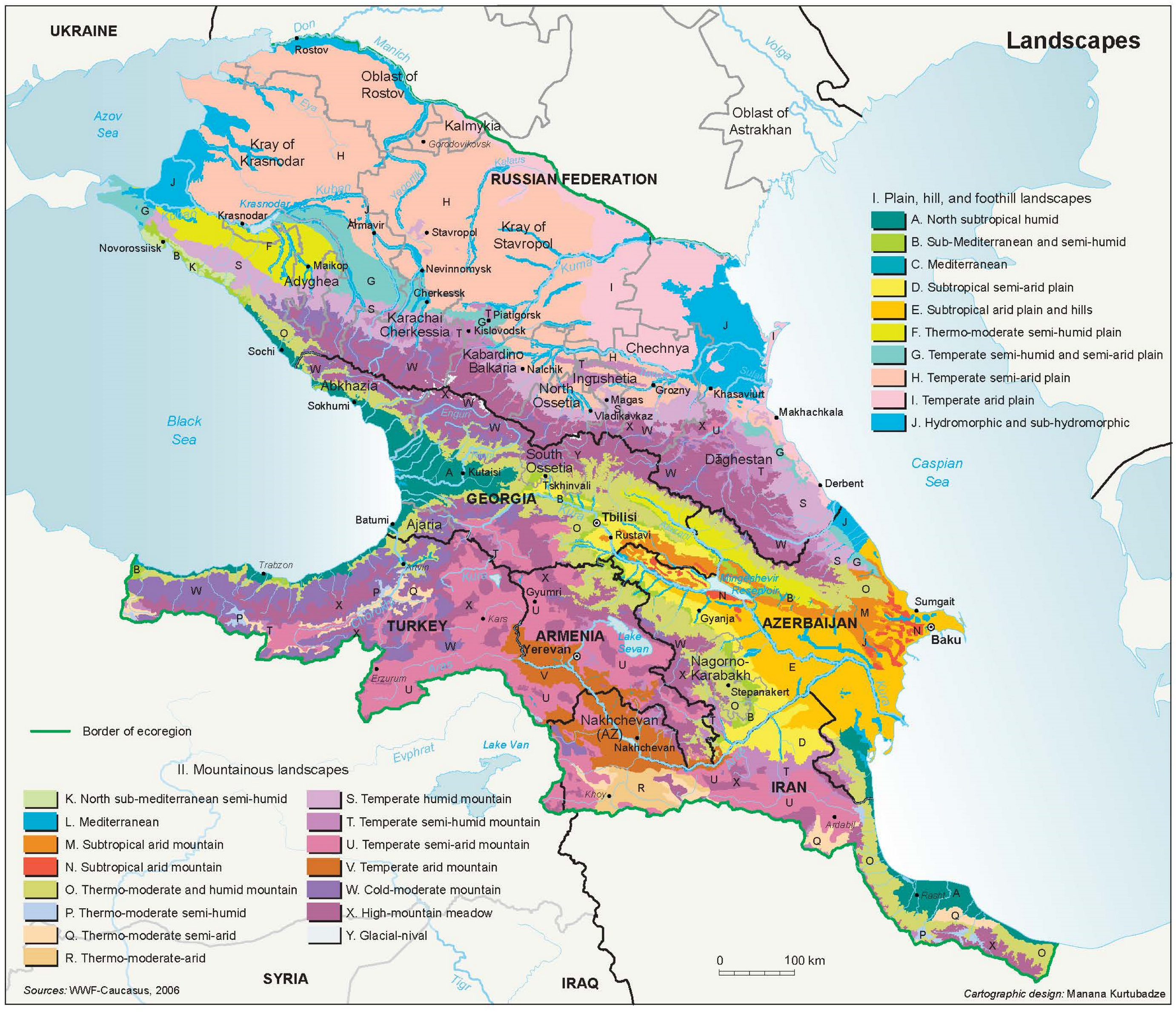
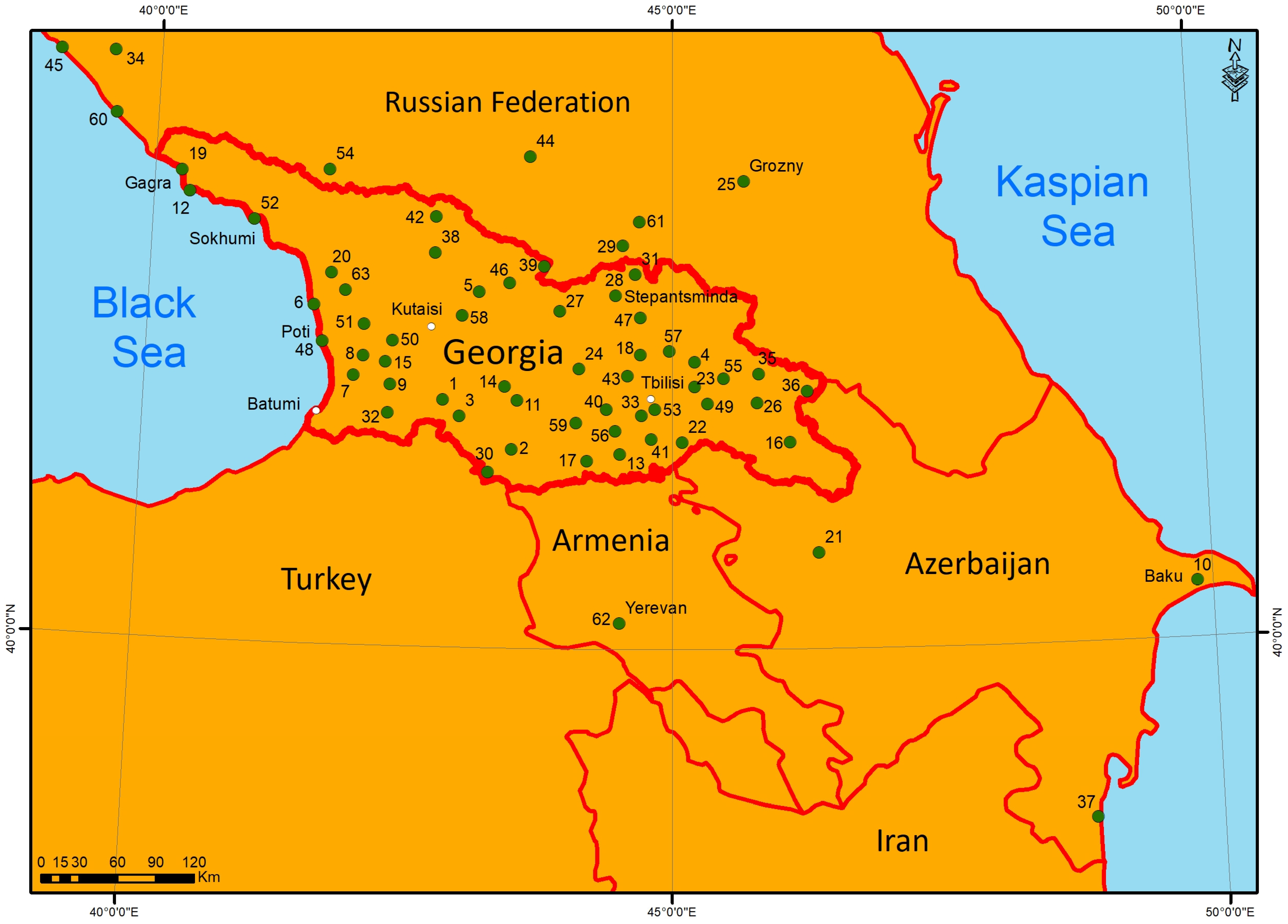
2.1. Study Area and Data Sources

The concept of landscape differentiation in the Caucasus was developed at the Laboratory of Aerospace Methods for Research of Natural Conditions of Ivane Javakhishvili Tbilisi State University [16,17,18], leading to the creation of a comprehensive landscape map of the region (scale 1:1,000,000) [15]. This landscape map was compiled using various cartographic materials, including field landscape photography, aerial surveys, satellite imagery, and thematic maps, which collectively account for the structural–petrographic features, local conditions, and anthropogenic factors influencing each landscape unit.

The highest qualification unit on the landscape map of the Caucasus is the landscape class. N. Beruchashvili [15] distinguishes 2 classes: I-plain and hilly landscapes and II- mountain landscapes. Landscape classes are divided into types and then subtypes (

Table 1. Caucasus landscape classification and the meteorological stations located there.

Classes	Types	Subtypes	Meteorological Stations (Numbering as in Table 2)
Plain and hilly landscapes	Subtropical humid plains and hills.	Colchis forest, Hyrcanian forest, and shrubland landscapes.	6. Anaklia 7. Anaseuli 8. Atsana 12. Bitchvinta 15. Dablatsikhe 20. Gali 39. Mamisoni 48. Poti 50. Samtredia 51. Senaki 52. Sokhumi 58. Tkibuli 63. Zugdidi
	Submediterranean subhumid plains and hills	Colchis transitional forest; submediterranean forest itself, arid sparse forest; temperately warm transitional subhumid forest.	4.  Akhmeta 24. Gori 49. Sagarejo 53. Tbilisi 55. Telavi 60. Tuapse
	Subtropical subarid plains and hills	Steppe and semi-desert.	16. Dedoplistskaro 21. Ganja 22. Gardabani 41. Marneuli 43. Mukhrani
	Subtropical arid plains and hills	Desert and semi-desert.	10. Baku
	Temperately warm subhumid landscapes of the plains.	Subtropical to transitional forest; Temperate to transitional forest.	13. Bolnisi 26. Gurjaani 36. Lagodekhi 35. Kvareli
	Temperately warm and temperate subhumid of the plains and hills	Meadows, steppes, shrublands, and forest-steppes.
	Temperately warm and temperate subarid landscapes of the plains and hills	Steppes	25. Grozny 61. Vladikavkaz 44. Nalchik 34. Krasnodar
	Temperately arid landscapes of the plains	Deserts and semi-deserts.
	Hydromorphic and subhydromorphic landscapes	Subtypes of swamps, salt marshes, and meadows.
Mountain landscapes	Mountain submediterranean subhumid landscapes.	Humid subtropical and temperate warm transitional low mountain forest, and mountain Mediterranean transitional forest, xerophytic	45. Novorossiysk
	Mountain subtropical subarid landscapes	Steppe, xerophytic, and arid sparse forest subtype.
	Mountain subtropical arid landscapes:	Semi-desert and desert subtypes
	Mountain temperate warm humid landscapes.	Lower mountain Colchis forest; middle mountain Colchis forest; lower mountain Hyrcanian forest; middle mountain Hyrcanian forest; lower montane forest; transitional to subhumid lower montane forest; middle montane forest.	1.  Abastumani 5.  Ambrolauri 9.  Bakhmaro 14. Borjomi 19. Gagra 23. Gombori 18. Dusheti 56. Tetri Tskaro 57. Tianeti 33. Kojori 38. Lentekhi 46. Oni 47. Pasanauri 32. Khulo 27. Java 40. Manglisi
	Mountain temperate humid landscapes.	Lower mountain forest and middle mountain forest.
	Mountain temperate subhumid landscapes.	Moderately warm transitional middle mountain xerophytic, arid sparse forest, phrygana, meadow-steppe; moderately warm transitional mountain forest, steppe; low mountain forest, forest-bush, meadows and steppes; medium mountain meadows, steppes, meadow-steppes, shiblyak and phrygana	2.  Akhalkalaki 17. Dmanisi 30. Kartsakhi 59. Tsalka
	Mountain temperate subarid landscapes.	Moderately warm transitional mountain steppes, meadows, phrygana, and shiblyak; moderately warm transitional middle mountain steppes and shiblyak, high mountain steppes and meadows transitional into mountain meadows; plateau with steppe and meadow-steppe vegetation; mountain depression steppes and shiblyak.	3.  Akhaltsikhe 29. Karmadon 54. Teberda
	Mountain temperate arid landscapes.	Lower mountain deserts and semi-deserts; mountain depression deserts	62. Yerevan
	Mountain temperate cold landscapes:	medium mountain dark coniferous forest; upper mountain forest.	42. Mestia 11. Bakuriani
	High mountain meadows.	high mountain subalpine forest-shrub-meadows; high mountain alpine shrub-meadows; high mountain subnival and glacial–nival landscapes.	39. Mamisoni 28. Jvari Pass 31. Kazbegi

). The same table indicates which meteorological station is located in which landscape.

Landscape subtypes are divided into genera and species. According to N. Beruchashvili [19], 152 landscape genera are recorded in the Caucasus. We used landscape types and, in some cases, subtypes in our study.

Table 2. Location of meteorological stations.

ID	NAME	Lat	Long	Elevation (m)
1	Abastumani	41.75	42.83	1329
2	Akhalkalaki	41.41	43.49	1721
3	Akhaltsikhe	41.64	42.99	1001
4	Akhmeta	42.04	45.21	571
5	Ambrolauri	42.52	43.15	577
6	Anaklia	42.40	41.58	7
7	Anaseuli	41.91	41.98	135
8	Atsana	42.05	42.07	199
9	Bakhmaro	41.85	42.33	1920
10	Baku	40.39	49.86	28
11	Bakuriani	41.75	43.53	1662
12	Bitchvinta	43.16	40.34	7
13	Bolnisi	41.38	44.50	641
14	Borjomi	41.85	43.41	820
15	Dablatsikhe	42.01	42.27	264
16	Dedoplistskaro	41.46	46.11	811
17	Dmanisi	41.33	44.20	1243
18	Dusheti	42.09	44.70	867
19	Gagra	43.30	40.26	9
20	Gali	42.63	41.74	55
21	Ganja	40.68	46.36	392
22	Gardabani	41.46	45.09	314
23	Gombori	41.86	45.21	1036
24	Gori	41.98	44.11	606
25	Grozny	43.32	45.69	128
26	Gurjaani	41.74	45.80	420
27	Java	42.39	43.92	1078
28	Jvari Pass	42.51	44.45	2409
29	Karmadon	42.86	44.52	1265
30	Kartsakhi	41.24	43.27	1855
31	Kazbegi	42.65	44.64	1762
32	Khulo	41.65	42.31	981
33	Kojori	41.66	44.70	1251
34	Krasnodar	45.04	38.97	25
35	Kvareli	41.95	45.82	418
36	Lagodekhi	41.82	46.27	438
37	Lenkoran	38.76	48.85	−21
38	Lentekhi	42.79	42.72	730
39	Mamisoni	42.71	43.77	2550
40	Manglisi	41.70	44.38	1197
41	Marneuli	41.49	44.80	429
42	Mestia	43.04	42.72	1408
43	Mukhrani	41.93	44.58	549
44	Nalchik	43.48	43.62	483
45	Novorossiysk	44.72	37.77	30
46	Oni	42.58	43.44	800
47	Pasanauri	42.35	44.69	1076
48	Poti	42.14	41.67	9
49	Sagarejo	41.74	45.33	755
50	Samtredia	42.16	42.34	26
51	Senaki	42.27	42.06	34
52	Sokhumi	42.98	40.98	8
53	Tbilisi	41.70	44.83	492
54	Teberda	43.36	41.68	1428
55	Telavi	41.92	45.48	690
56	Tetri Tskaro	41.54	44.46	1168
57	Tianeti	42.11	44.97	1110
58	Tkibuli	42.35	43.00	577
59	Tsalka	41.60	44.09	1471
60	Tuapse	44.10	39.07	12
61	Vladikavkaz	43.03	44.68	704
62	Yerevan	40.18	44.51	1014
63	Zugdidi	42.51	41.87	112

presents the geographical coordinates of meteorological stations, and Figure 2 shows the spatial distribution of meteorological stations. Meteorological stations are numbered on the map by Table 2.

The spatial distribution of the meteorological stations used in this study is illustrated in Figure 2.

Air temperature and precipitation data were obtained from the National Environmental Agency of Georgia, supplemented by the European Climate Assessment and Dataset (ECA&D) and a regional climate simulation [20].

Station metadata, including elevation, location, and observation duration, were verified for quality control and utilized to investigate the seasonal temperature and precipitation patterns in the Caucasus landscapes for 1950–2022.

2.2. Methods

To analyze temperature trends, linear regression analysis was employed. The coefficient of determination (R²) was used to quantify the proportion of variance in temperature explained by the temporal trend, while p-values were calculated to assess the statistical significance of the regression coefficients. Vertical lapse rates (°C per 100 m) were determined by regressing monthly mean temperatures against the elevation of meteorological stations. Temperature inversion events were identified when the vertical temperature gradient became positive, indicating an increase in temperature with altitude. The magnitude of these inversions was quantified on a seasonal basis.

To construct the elevation–temperature curves, we used locally weighted scatterplot smoothing, a non-parametric regression technique suitable for capturing non-linear relationships without assuming a specific functional form. The method was applied to station-level monthly and annual mean temperatures plotted against elevation, allowing for localized trends in temperature lapse rate to emerge [21].

Elevation intervals were sampled uniformly along the range of observed station elevations (0 to 3600 m), and the smoothing bandwidth was selected to balance fidelity and generalization. No additional weighting based on station density was applied, as the objective was to reflect general climatic structure across landscapes, not regional observation bias.

Prior to curve fitting, basic quality control procedures were implemented: data were screened for outliers using the interquartile range (IQR) method, where values lying more than 1.5 × IQR from the quartiles were flagged and manually verified using station metadata. Stations with missing or clearly erroneous data (e.g., implausible temperature–elevation mismatches) were excluded.

This approach ensured a robust and transparent derivation of lapse-rate profiles representative of the region’s complex topography and climatic gradients.

To assess temperature variability across the diverse landscape types of the Caucasus region, we computed summary statistics for monthly and annual mean air temperature, including the mean, standard deviation (SD), and coefficient of variation (CV). These metrics provide a quantitative understanding of both central tendency and relative variability in thermal regimes.

Precipitation regimes were analyzed by aggregating monthly totals to construct annual precipitation curves per landscape type. To validate the observed seasonal precipitation patterns across different landscape types, we applied the Mann-Kendall trend test and Sen’s slope estimator to monthly and seasonal precipitation series for 1950–2022. These methods are well-established for detecting monotonic trends in hydroclimatic time series and are robust to non-normal data distributions and outliers [22,23].

3. Results and Discussion

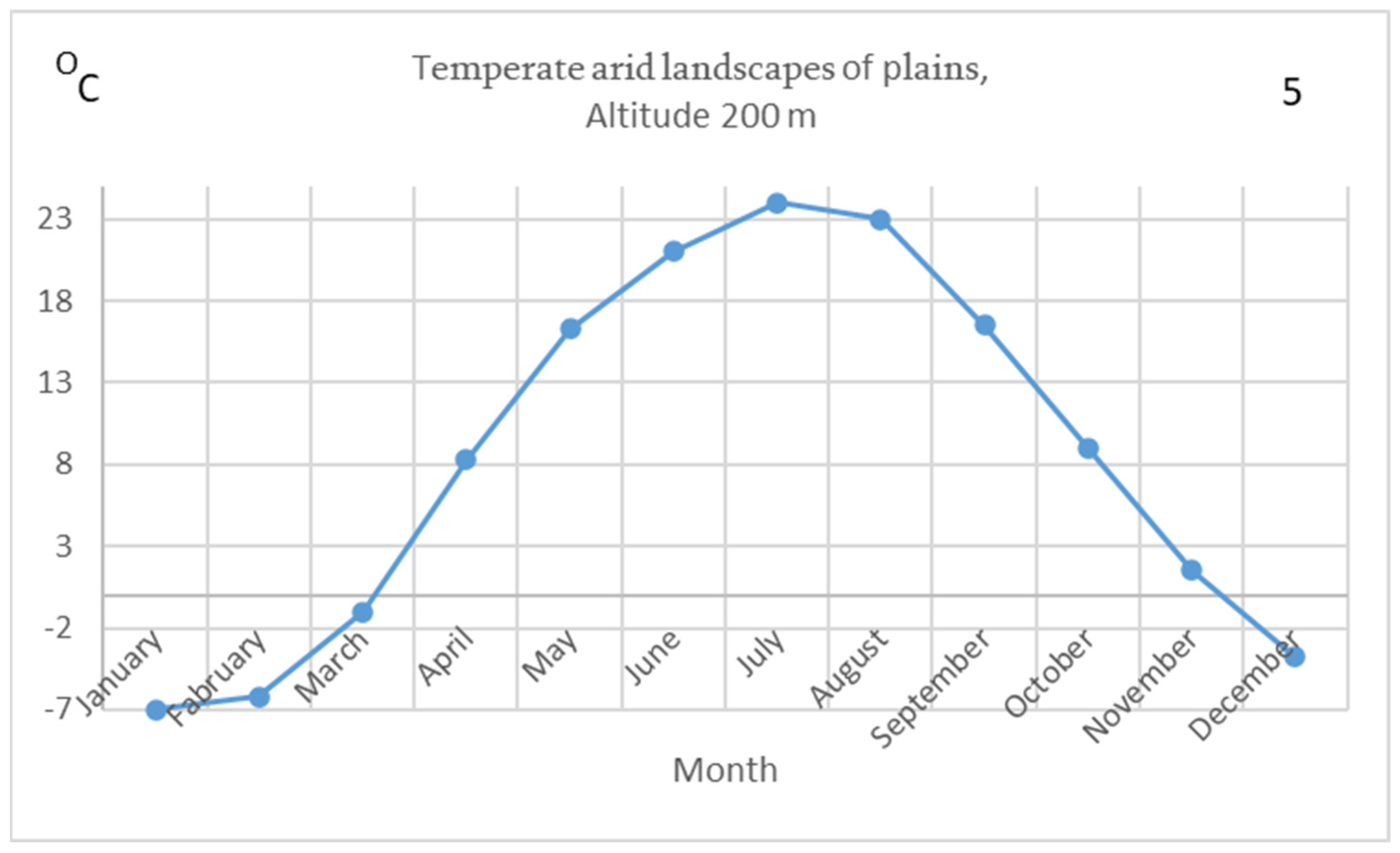
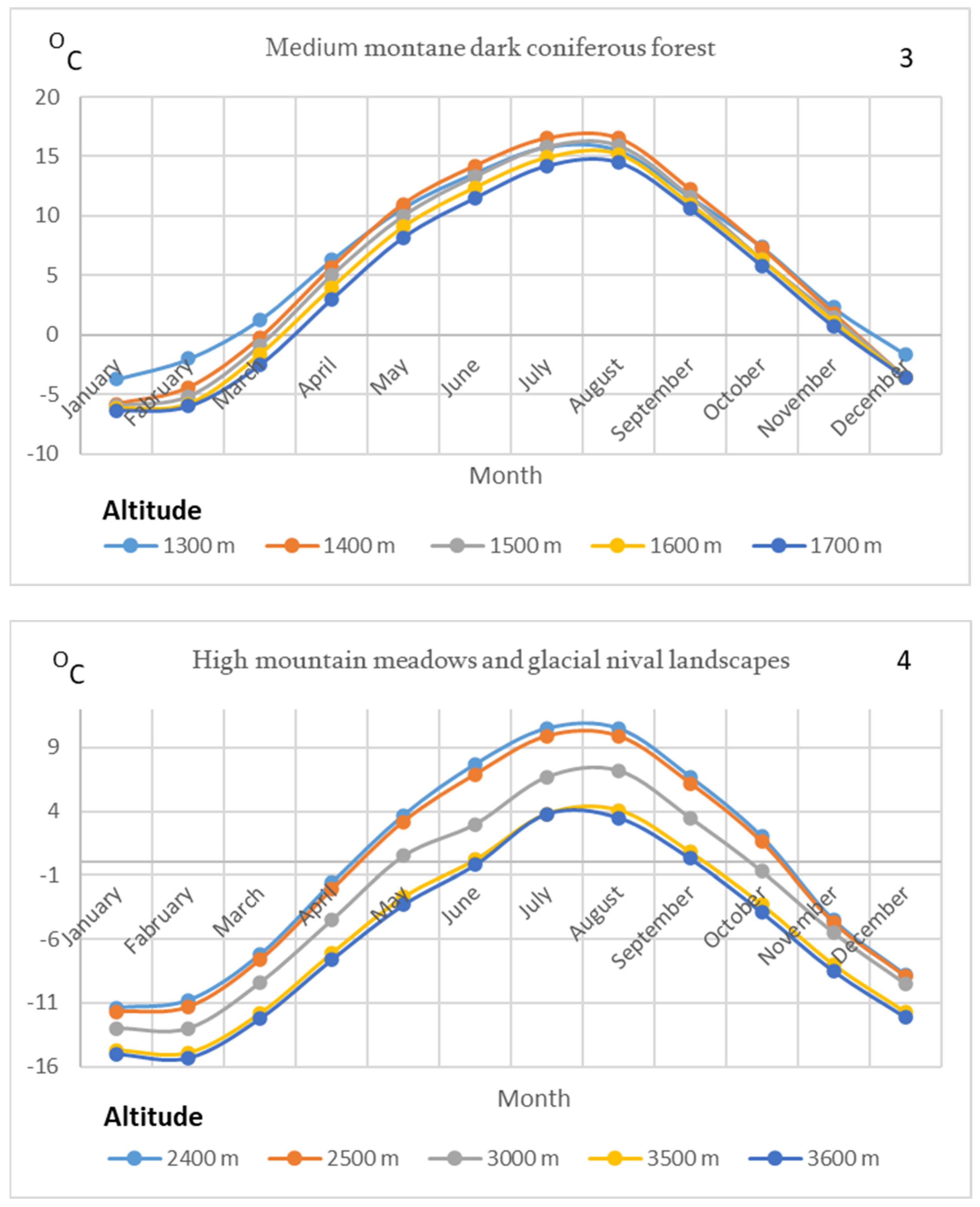
3.1. Changes in the Annual Course of Air Temperature in Different Landscape Conditions

The climate is the most important factor in the formation of natural landscapes. At the same time, the type of natural landscape itself contributes to the formation of a specific climatic regime, particularly at the microclimate level. For instance, forests, swamps, water reservoirs, and urban environments exhibit distinctive microclimates. Therefore, a reciprocal relationship exists between the climate and natural landscapes. A similar type of natural landscape may be distributed across different geographical regions of the Caucasus, spanning various elevation zones. This applies equally to mountainous and lowland landscapes. For example, subtropical humid landscapes of the plains and hills are commonly found up to 600 m above sea level; submediterranean subhumid landscapes occur between 200 and 800 m; and moderately warm and temperate subarid landscapes of the plains and hills are observed up to 700 m above sea level.

Figure 3 and Figure 4 present the monthly air temperature courses in plains, hilly, and mountain landscapes according to the altitude. In most types of natural landscapes of the Caucasus, the temperature minimum is established in January, except glacial–nival landscapes and high mountain meadows, where the minimum temperature is in February. As for the maximum, in humid landscapes, it is mainly in August, and in the rest of the landscapes, it is in July. This indicates the inertia of humid landscapes. For the same reason, after wintering, arid landscapes warm up faster than humid ones. In particular, in plain and hilly subtropical humid landscapes, the March temperature is 1.5–2.2 °C higher than the average February temperature.

This difference is 2.4–4.0 °C for submediterranean subhumid landscapes of plains and hills, 3.1–4.4 °C for subtropical subarid landscapes of plains and hills, 5.1–6.0 °C for moderately warm and temperate subarid landscapes of plains and hills, and so on. A similar ratio is found in the mountains. In humid landscapes of the lower and middle mountain Colchis forest, the March temperature exceeds the February temperature by 3–4 °C and in temperate arid mountain landscapes by 5–6 °C. Cooling also follows the same pattern. After summer, the temperature drops faster in relatively arid landscapes than in humid ones.

The difference in subtropical humid landscapes of plains and hills is approximately 3 °C, in submediterranean subhumid and subtropical subarid landscapes of plains and hills it is 4.0–4.5 °C, in moderately warm and temperate landscapes of plains and hills it is 5.0–5.5 °C, in humid landscapes of the Colchis forest it is 2.0–4.0 °C, and in temperate arid landscapes of mountains it is 4.0–5.5 °C.

These differences in the timing and amplitude of seasonal temperature maxima and minima were observed across landscape types. Specifically, arid and subarid lowland regions tend to experience earlier warming in spring and quicker cooling in autumn, whereas humid and montane landscapes exhibit a lag in warming, often showing March as warmer than February, and a more gradual temperature decline in autumn.

The concept of thermal inertia—defined as a material’s resistance to temperature change in response to heat input or loss—is relevant when interpreting the seasonal behavior of different landscape types. In climatological terms, thermal inertia is influenced by surface heat capacity, thermal conductivity, and moisture content, all of which vary significantly across landscapes [24,25]. Forested and humid subtropical landscapes, which feature dense vegetation cover, higher soil moisture, and organic-rich soils, exhibit greater thermal inertia and thus tend to warm and cool more slowly than arid or sparsely vegetated landscapes, where low moisture and bare soil conditions lead to faster thermal response. This behavior is consistent with the observed seasonal lag in temperature peaks and is also supported by studies [26] that link land surface properties with surface temperature dynamics.

Although our study does not directly model surface energy fluxes or heat storage, the seasonal temperature distribution across different landscape classes indirectly reflects differential thermal responses due to landscape-specific physical properties.

Table 3. Statistics of monthly and annual mean temperature across different landscapes.

Landscape Type, Subtypes	Statistical Parameter	Months
		January	February	March	April	May	June	July	August	September	October	November	December	Year
Subtropical humid of plains and hills	T (°C)	3.70	4.5	6.69	11.3	16.4	19.4	21.7	21.9	19	15	10	5.9	13
	SD (°C)	1.62	1.5	1.62	0.92	0.73	1.07	1.10	1.43	0.9	0.9	1	1.4	0.9
	CV, (%)	43.9	32	24.3	8.11	4.44	5.50	5.07	6.53	4.5	6.3	10	23	7.1
Submediterranean subhumid of plains and hills	T (°C)	0.36	1.64	5.4	10.8	16.0	19.9	22.9	22.8	18.4	12.9	6.88	2.4	12
	SD (°C)	0.46	0.61	0.85	0.70	0.81	0.88	0.95	1.00	0.97	0.71	0.53	0.32	0.7
	CV, (%)	128	37.2	15.8	6.48	5.04	4.45	4.14	4.40	5.24	5.48	7.65	13.1	6.2
Subtropical subarid of plains and hills	T (°C)	−1.3	0.40	4.2	9.8	15	18.7	22	21.9	17.5	11.6	5.68	0.88	11
	SD (°C)	0.22	0.26	0.87	0.61	0.52	0.35	0.51	0.22	0.44	0.64	0.56	0.30	0.3
	CV, (%)	-	64.5	20.7	6.22	3.42	1.87	2.27	1.01	2.51	5.48	9.80	34.1	3.6
Temperate warm, and temperate subarid of plains and hills	T (°C)	−4.1	−2.9	2.38	9.13	15.4	19.4	22	21.6	16.2	10.2	3.49	−1.4	9.4
	SD (°C)	1.11	1.02	0.96	0.90	1.17	1.29	1.48	1.42	1.08	0.98	1.02	1.05	1.0
	CV, (%)	-	-	40.4	9.83	7.56	6.66	6.71	6.54	6.64	9.52	29.2	-	11
The lower and middle montane Colchis forest humid	T (°C)	−2.7	−2	1.54	6.81	11.9	15.1	17.1	17.6	14.1	9.56	4.08	−0.4	7.8
	SD (°C)	1.83	2.03	2.50	2.87	3.06	2.86	2.86	2.86	2.22	1.70	1.90	1.18	2.3
	CV, (%)			162	42	25.6	18.9	16.7	16.2	15.7	17.7	46.6		29
Mountain moderately arid	T (°C)	−1.8	−0.2	5.53	12	16.9	21.1	24.8	24.6	20.4	14.4	8.37	0.60	12
	SD (°C)	1.98	2.24	1.69	1.08	1.10	1.10	0.82	0.50	0.43	0.63	0.18	1.73	1.2
	CV, (%)	-	-	30.6	9.00	6.53	5.23	3.31	2.01	2.12	4.32	2.15	288	9.5
Medium montane dark coniferous forest	T (°C)	−5.6	−4.7	−0.78	4.8	9.8	13	15.4	15.5	11.4	6.62	1.48	−3.2	5.4
	SD (°C)	1.10	1.62	1.44	1.32	1.16	1.06	0.90	0.75	0.62	0.70	0.62	0.89	0.8
	CV, (%)	-	-	-	27.5	11.7	8.16	5.80	4.83	5.41	10.5	41.7	-	14
High mountain meadows and glacial nival landscapes	T (°C)	−13	−13	−9.64	−4.58	0.28	3.52	6.94	7.04	3.5	−0.9	−6.3	−10	−3
	SD (°C)	1.66	2.04	2.31	2.76	3.24	3.68	3.21	3.22	2.96	2.71	1.88	1.58	2.5
	CV, (%)	-	-	-	-	997	104	46.2	45.7	84.5	-	-	-	-

presents detailed statistics of monthly and annual mean air temperatures across diverse landscape types in the Caucasus region, offering insight into spatial and temporal thermal variability. Subtropical humid plains and hills exhibit the warmest annual average temperature (13 °C), with relatively low interannual variability (CV = 7.1%). In contrast, the high mountain meadows and glacial–nival landscapes experience the coldest conditions (annual mean = −3 °C) and the highest variability (SD = 2.5 °C), reflecting the influence of elevation and exposure. The coefficient of variation (CV) in January temperatures reaches extreme values in colder landscapes, such as 128% in submediterranean subhumid plains and 162% in Colchic montane forests, indicating high interannual variability in winter. Seasonal contrasts are also apparent: for example, summer months (June–August) show lower CVs across all landscapes, suggesting more stable thermal regimes during the warm season. Moderately arid mountain areas and temperate-subarid plains demonstrate pronounced warming in summer, with peak temperatures exceeding 24 °C in July–August, whereas forested and alpine zones maintain cooler profiles throughout the year. These patterns highlight the significant influence of topography, continentality, and vegetation cover on temperature distributions, which is crucial for interpreting climate impacts in this highly heterogeneous region.

3.2. Temperature Inversion in Different Landscape Conditions

Temperature inversions, situations where air temperature increases with altitude, play a critical role in shaping local weather, air quality, and climate processes. These events are especially common in valleys, basins, and coastal regions where stable atmospheric layers form due to terrain-induced cooling and maritime influences [27,28,29,30]. Studies from the Alps and Andes have shown that such inversions can suppress vertical mixing, trap pollutants, and influence precipitation regimes [31,32,33].

In mountainous regions like the Caucasus, vertical air temperature gradients (lapse rates) typically average −0.6 °C per 100 m of elevation gain, although local conditions such as vegetation cover, humidity, and proximity to the Black Sea cause significant deviations [34]. Our analysis in

Table 4. Monthly and annual values of vertical air temperature gradients °C/100 m.

Landscape Type, SubtypeF	Month												Year
	January	February	March	April	May	June	July	August	September	October	November	December		SD	95% CI Lower Upper
Subtropical humid of plains and hills	0.75	0.66	0.70	0.26	0.05	0.45	0.45	0.45	0.40	0.45	0.46	0.65	0.42	0.20	0.28
															0.68
Submediterranean subhumid of plains and hills	0.25	0.49	0.52	0.44	0.50	0.52	0.60	0.60	0.60	0.42	0.41	0.20	0.42	0.14	0.29
															0.57
Subtropical subarid of plains and hills	0.12	0.15	0.50	0.35	0.30	0.20	0.20	0.12	0.25	0.30	0.30	0.18	0.22	0.10	0.14
															0.34
Temperate warm and temperate subarid of plains and hills	0.50	0.47	0.47	0.40	0.50	0.47	0.53	0.51	0.47	0.41	0.46	0.43	0.46	0.06	0.40
															0.52
Low and middle montane Colchis forest humid	0.55	0.61	0.74	0.35	0.91	0.87	0.83	0.87	0.65	0.28	0.58	0.36	0.69	0.20	0.36
															0.76
Mountain temperate arid	0.91	1.30	0.92	0.50	0.52	0.52	0.33	0.23	0.20	0.40	0.40	0.80	0.55	0.31	0.18
															0.79
Middle montane dark coniferous forest	0.67	1.0	0.95	0.82	0.62	0.52	0.40	0.25	0.25	0.40	0.40	0.50	0.66	0.21	0.37
															0.78
High montane meadows. glacial nival landscapes	0.30	0.37	0.42	0.50	0.58	0.61	0.46	0.58	0.53	0.50	0.37	0.27	0.49	0.10	0.35
															0.53

reveals that these gradients vary strongly by landscape type and season.

In subtropical humid plains and hills, lapse rates are steep in winter (0.75 °C/100 m in January) but decrease sharply in spring, reaching near-inversion values in May (0.05 °C/100 m). This pattern suggests the presence of seasonal inversion layers caused by the advection of warm, stable air from the Black Sea. Historical research by in 1978 [35] noted this phenomenon in western Georgia, attributing it to springtime maritime air masses. He reported inversion layers of ~70 m thickness and a modest magnitude of 0.3 °C [35], whereas our study identifies stronger inversions (100–150 m thick; 0.5–2.0 °C). Such a significant difference between our data and E. Elizbarashvili’s data is explained by the fact that E. Elizbarashvili’s conclusions were based on the analysis of observational data from meteorological stations in western Georgia, and the influence of the landscape type was leveled. The time period factor is also important, with significant climate changes observed since 1978.

Montane zones, especially the Colchis forest, and dark coniferous forest landscapes exhibit strong lapse rates (≥0.66 °C/100 m annually), with seasonal peaks exceeding 0.9 °C/100 m. This suggests active convective mixing and orographic lifting in these humid, forested regions. In contrast, subarid lowlands show the lowest annual gradients (~0.22 °C/100 m), indicative of stable air masses and minimal vertical mixing.

High-elevation zones, including glacial–nival landscapes, show moderate lapse rates that increase gradually from winter to summer (0.3–0.6 °C/100 m), likely driven by snow-albedo feedbacks and reduced insolation.

Additionally, terrain-induced cold air drainage—katabatic flows—contributes to temperature inversions in valleys and basins, particularly under clear skies and calm wind conditions [36,37].

These localized dynamics result in nocturnal cold-air pooling that reinforces inversion strength and persistence.

Annual vertical air temperature gradients across different landscape types reveal considerable spatial variability, reflecting the complex interactions between topography, land cover, and regional climatic regimes. The steepest negative lapse rates (i.e., strongest decrease in temperature with elevation) are observed in the low and middle montane humid Colchis forest (0.69 °C/100 m, SD = 0.20) and middle montane dark coniferous forest (0.66 °C/100 m, SD = 0.21), indicating a pronounced cooling effect with elevation in densely forested and humid mountainous zones. Similarly, Mountain temperate arid landscapes exhibit a high gradient (0.55 °C/100 m, SD = 0.31), although with the largest variability (95% CI: 0.18–0.79), possibly due to heterogeneous terrain and sparse vegetation cover that affects local thermal dynamics.

More moderate gradients are recorded in the high montane meadows and glacial–nival landscapes (0.49 °C/100 m, SD = 0.10) and temperate warm and temperate subarid plains and hills (0.46 °C/100 m, SD = 0.06), with the latter showing the narrowest confidence interval (0.40–0.52), suggesting relatively stable temperature–elevation relationships in these areas. The subtropical humid and submediterranean subhumid plains and hills display gradients of 0.42 °C/100 m, though the former exhibits more variability (SD = 0.20 vs. 0.14). The lowest vertical gradient is found in the subtropical subarid plains and hills (0.22 °C/100 m, SD = 0.10), indicating weaker cooling with altitude in these warmer, drier regions.

In conclusion, understanding landscape-specific patterns of temperature inversion and lapse rates is vital for climate modeling, ecosystem monitoring, agricultural planning, and air quality management in mountainous regions.

3.3. Precipitation Annual Course in Different Landscape Conditions

The annual precipitation course is characterized by great diversity (

Table 5. Characterization of the annual course of precipitation.

Landscape Type, Subtype	Main Maximum, Month, Quantity, mm	Main Minimum, Month, Quantity mm	Secondary Maximum, Month, Quantity, mm	Secondary Minimum, Month, Quantity, mm
Plains and hills subtropical humid	September–February, 140–300	May–August, 60–150	-	-
Plains and hills sub Mediterranean subhumid	May, 90–150	December–January, 20–40	-	-
Plains and hills subtropical subarid	May, 90–100	January, 25–30	October, 50–55	-
Plains temperate subhumid	May, 150	January, 40	September, 120	-
Plains and hills subtropical arid	November, 35–40	August, 5–10	December, 30–35	September, 5–10
Plains temperate arid	June, 40–45	February, 20–30	December, 40–45	September, 20–30
Mountain temperate warm humid	May–June, 90–140	December–January, 20–40	-	-
Mountain temperate cold	May–June, October, 80–120	December–February, 20–70	-	-
High mountain meadows	May, 170–220	January, 100	-	July, 90

). The annual course of precipitation is especially diverse in subtropical humid landscapes of plains and hills, which are generally characterized by a large amount of precipitation. Here, the annual course of precipitation has a maximum in autumn or winter, and the monthly total is 140–300 mm. The minimum precipitation falls mainly in May and in some areas during some summer months and amounts to 60–150 mm.

In the submediterranean subhumid landscapes of plains and hills, the maximum monthly precipitation totals fall in May (90–150 mm), and the minimum in January, possibly December (20–40 mm). Almost the same type of pattern of precipitation annual course—maximum in May and minimum in January—is characteristic of the subtropical subarid landscapes of plains and hills, with the difference that in the latter, a second, weakly expressed maximum occurs in October (50–55 mm). The main maximum is approximately twice as high as the secondary maximum, and the minimum is 25–30 mm.

For moderately warm subhumid landscapes of plains, the maximum precipitation is about 150 mm in May, and the minimum of 40 mm is in January. The secondary maximum is well expressed here and reaches 120 mm in September. In the subtropical arid landscapes of the plains and hills, the maximum of precipitation falls in November and is 35–40 mm, and the minimum corresponds to August (5–10 mm).

In the moderately warm and temperate landscapes of the plains and hills, the maximum of precipitation falls mainly in June (80–170 mm) and the minimum in January-February (20–40 mm). In lowland areas, a second maximum of the same magnitude is observed in December, and the minimum is shifted to September. The temperate arid landscapes of the plains are characterized by two equally pronounced maxima in June and December (40–45 mm) and also two equally pronounced minima in February and September (20–30 mm).

In mountain landscapes, the establishment of maxima and minima in the annual course of precipitation often alternates. For example, in the transitional landscapes of low and medium mountain forests to humid ones, the maximum precipitation is possible in May and June (90–140 mm), and the minimum is in December or January (20–40 mm). In medium mountain coniferous forest landscapes, except for May and June, the maximum precipitation can occur in October (80–120 mm) and the minimum in any winter month (40–70 mm).

Secondary maxima in precipitation observed in several landscape types—particularly in October and December—are attributed to distinct regional climatological drivers. During these months, the influence of Mediterranean cyclones intensifies across the Caucasus region, particularly affecting western and southern Georgia. These cyclones often follow southwesterly trajectories and are associated with warm, moist air masses that, upon encountering the Greater and Lesser Caucasus ranges, generate orographic uplift and enhanced precipitation, especially in subtropical and submediterranean landscapes. In addition to cyclone-induced rainfall, synoptic-scale frontal passages become more frequent during autumn, contributing to precipitation variability. October maxima are also linked to residual surface heating and increased atmospheric instability, which may support convective activity in lowland and foothill zones. December peaks, observed mainly in arid and semi-arid regions, often result from episodic frontal intrusions associated with low-pressure systems from the Black Sea basin. These processes collectively shape the secondary precipitation peaks and underscore the importance of mesoscale and synoptic circulation patterns in modulating the region’s hydrological seasonality [4,38,39,40].

Conversely, some landscape types exhibit a secondary minimum of precipitation in September, notably in temperate arid and semi-arid plains. This decline is attributable to the seasonal weakening of both convective activity and frontal systems during the transition from summer to autumn. In September, the South Caucasus frequently experiences a phase of atmospheric stability characterized by high-pressure dominance, reduced humidity, and limited cyclone incursions. These conditions suppress precipitation generation, particularly in rain-shadowed or interior lowland areas, where orographic enhancement is minimal. Such September dry spells have been documented in regional climate analyses [4] and are further reinforced by the subtropical anticyclone belt’s lingering influence over the region during early autumn.

To validate the observed seasonal precipitation patterns across different landscape types, we applied the Mann-Kendall trend test and Sen’s slope estimator to monthly and seasonal precipitation series for the period 1950–2022. These methods are well-established for detecting monotonic trends in hydroclimatic time series and are robust to non-normal data distributions and outliers [41,42,43]. In humid lowland landscapes (e.g., Colchis Plain), autumn and winter precipitation maxima are statistically significant (p < 0.05), with positive Sen’s slopes ranging from +1.1 to +2.4 mm/year, confirming long-term intensification of cool-season precipitation.

In semi-arid and subarid landscapes of the eastern lowlands, spring precipitation—historically peaking in April–May—shows a significant decreasing trend, with Z-scores between −2.0 and −2.6 and Sen’s slopes ranging from −0.9 to −1.4 mm/year, suggesting a growing seasonal water deficit.

In montane forest zones, summer and autumn precipitation trends were mixed and mostly not statistically significant, indicating high interannual variability but no robust monotonic changes.

For high-elevation zones (>2500 m), precipitation trends were not significant, though the amplitude of variability has increased since the 1980s, likely reflecting changing atmospheric circulation and snow-rain partitioning.

Although this study primarily focuses on average seasonal climate characteristics, the observed seasonal shifts and variability in precipitation and temperature are closely related to the occurrence of extreme events. For example, increasing spring-to-summer temperature gradients in arid lowland areas may exacerbate heatwave risks, while intensification of autumn–winter precipitation in humid zones aligns with recent observations of extreme rainfall events and flash flooding [9].

A follow-up study will analyze trends in temperature and precipitation extremes using percentile-based and threshold indices from the ETCCDI (Expert Team on Climate Change Detection and Indices) framework.

3.4. Limitations and Future Research

Despite offering valuable insights into the climatic characteristics of various landscape types in the Caucasus, this study has several limitations that must be acknowledged. The landscape classification used in this study is based on foundational work developed in the 1980s–1990s. While it remains scientifically relevant, the landscape boundaries may not fully reflect current conditions due to changes in land use, vegetation cover, and anthropogenic influences. Integrating updated land cover datasets (e.g., CORINE, MODIS) and high-resolution remote sensing imagery in future research will allow for improved landscape–climate interaction assessments under present-day environmental conditions [44,45].

While the study uses a rich dataset from 63 meteorological stations and data from regional climate model simulations, temperature and precipitation trends are primarily evaluated using monthly or seasonal averages. Short-term extremes (e.g., heatwaves, flash droughts, intense rainfall events) and sub-daily variations are not addressed, which may be important under a changing climate regime [46].

The vertical temperature gradients (lapse rates) are analyzed using interpolated values across selected altitudes. However, finer-scale variations driven by slope orientation, local wind patterns, vegetation cover, or snowpack are not explicitly modeled. These microclimatic effects may lead to localized deviations from the generalized lapse rate trends. Inversion layers are discussed using climatological profiles, but detailed atmospheric sounding data (radiosonde) were not available. This restricts the analysis of inversion dynamics to inferred values, limiting precision [47].

Several lowland meteorological stations are located in or near urbanized areas, which may introduce biases due to urban heat island (UHI) effects [48]. These stations may record higher minimum temperatures, particularly during nighttime and winter inversions. While our analysis focuses on general landscape–climate patterns, future work should include UHI-corrected datasets or segregate urban and rural station trends to more accurately represent regional thermal regimes.

While this study provides a qualitative interpretation of how temperature and precipitation influence different landscape types across the Caucasus, it does not yet include a multivariate statistical assessment of these relationships. Future research should incorporate geospatial statistical approaches—such as generalized additive models (GAMs), machine learning classification (e.g., random forests), or principal component analysis (PCA)—to assess how climate variables, topographic factors, and land cover jointly explain landscape variability. Such methods would significantly enhance the scientific robustness of landscape–climate linkages and allow for better integration into vulnerability assessments and policy planning under future climate scenarios [49,50,51]. While our interpretation of thermal response is grounded in observed seasonal temperature variability, the study does not explicitly quantify thermal inertia using satellite-derived land surface temperature, soil moisture data, or energy balance models. Future research should integrate such datasets (e.g., MODIS LST, SMAP soil moisture) to model surface heat storage and fluxes more directly, enabling a more rigorous comparison across landscape types [52,53]. Future studies should consider integrating high-resolution satellite datasets (e.g., MODIS, CORINE), land surface temperature products, and ERA5 reanalysis to complement and verify ground-based observations [54].

Establishing or accessing additional high-elevation automatic weather stations will be critical for improving the spatial resolution of mountainous observations. Incorporating modern climate model outputs (e.g., regional downscaled projections) will also allow for the assessment of future landscape–climate interactions under different emission scenarios.

Future studies should quantify inversion metrics, such as the number of inversion days per year, average inversion depth, and temperature differential, stratified by land cover or elevation class. Incorporating these data into spatial overlays (e.g., GIS-based heatmaps) would significantly enhance understanding of mesoscale atmospheric processes and inform regional climate modeling and adaptation planning, particularly for agriculture, air quality management, and frost forecasting in complex terrain [55].

This study identifies landscape-dependent patterns in thermal regime characteristics, including differences in seasonal temperature variability and the occurrence of inversion-prone conditions. For example, montane and subalpine zones exhibit greater interseasonal variability and stronger thermal gradients, while lowland subtropical landscapes display more thermally stable conditions and minimal inversion effects. These distinctions have potential implications for agriculture, land use planning, and regional climate modeling.

4. Conclusions

This study presents a comprehensive analysis of seasonal air temperature, precipitation patterns, and vertical temperature gradients across the diverse landscape types of the Caucasus region using long-term observational data (1950–2022) from 63 meteorological stations and data from regional climate simulations. The results underscore the complex interplay between topography, climate, and landscape, highlighting several key findings relevant to both scientific understanding and regional climate adaptation strategies.

Seasonal and annual temperature distributions vary significantly by landscape type and elevation. Subtropical lowland landscapes exhibit the highest mean annual temperatures (above 13 °C), while glacial–nival and subnival zones display extreme cold conditions (as low as −10.8 °C). Temperature variability increases with elevation, with the highest relative fluctuations found in alpine and subalpine ecosystems. Thermal inertia in humid, forested zones causes seasonal lag in warming and cooling, which is particularly evident in delayed spring warming.

Lapse rates across the region reveal strong seasonal and spatial heterogeneity. Seasonal vertical gradients range from 0.24 to 0.57 °C per 100 m, with the highest values in montane forest zones. The presence of frequent and persistent temperature inversions—especially in spring and winter—is a defining feature of the region’s thermal regime. These inversions are most common in western lowlands and mountainous valleys and are strongly influenced by topographic confinement and radiative cooling.

Precipitation regimes are distinctly landscape-dependent. Humid lowland areas experience maxima in autumn and winter (140–300 mm/month), while arid lowlands peak in late autumn or spring. Some landscapes show secondary precipitation maxima in October or December, linked to Mediterranean cyclone activity and frontal systems. Conversely, a secondary precipitation minimum in September is observed in several arid zones, reflecting late-summer atmospheric stabilization.

Mann-Kendall trend analysis indicates statistically significant increases in autumn–winter precipitation in humid lowlands, while spring rainfall is declining in arid and semi-arid regions, suggesting the intensification of seasonal water deficits. Lapse rate variability, evaluated through standard deviation, IQR, and confidence intervals, confirms considerable heterogeneity in atmospheric stability across terrains, reinforcing the need for landscape-sensitive modeling approaches.

The findings emphasize the critical need to account for landscape-specific climate behavior in regional planning, agriculture, ecological forecasting, and climate change adaptation strategies. The strong spatial contrasts in thermal and hydrological regimes demonstrate that uniform climate assumptions across the Caucasus are inappropriate. High-elevation zones, in particular, are characterized by greater interannual variability and should be prioritized in future vulnerability assessments.

While this study focuses on observed historical climate patterns, the findings offer a critical reference for validating and downscaling future climate projections. Landscape-specific insights into lapse rates, inversion layers, and seasonal precipitation regimes can inform high-resolution regional climate modeling efforts. Integrating these findings into downscaled simulations will improve the accuracy of climate impact assessments, particularly for agriculture, hydrology, and hazard forecasting in the mountainous Caucasus region.

Overall, this study deepens our understanding of climate–landscape interactions in a region marked by extreme physiographic and climatic diversity. It provides a robust empirical foundation for future work on downscaled climate projections, land use planning, and ecosystem resilience in the face of ongoing and future climate change.

References

1. IPCC. Climate Change 2021: The Physical Science Basis; Contribution of Working Group I to the Sixth Assessment Report of the Intergovernmental Panel on Climate Change; Masson-Delmotte, V., Zhai, P., Pirani, A., Connors, S.L., Péan, C., Berger, S., Caud, N., Chen, Y., Goldfarb, L., Gomis, M.I., et al., Eds.; Cambridge University Press: Cambridge, UK, 2021. [Google Scholar] [CrossRef]
2. Soltani, K.; Amiri, A.; Ebtehaj, I.; Cheshmehghasabani, H.; Fazeli, S.; Gumiere, S.J.; Bonakdari, H. Advanced Forecasting of Drought Zones in Canada Using Deep Learning and CMIP6 Projections. Climate 2024, 12, 119. [Google Scholar] [CrossRef]
3. Rybak, O.O.; Rybak, E.A. Climate change in the south of Russia: Tendencies and possibilities for prediction. Sci. J. Kuban State Univ. 2015, 111, 3–18. [Google Scholar]
4. Tashilova, A.A.; Ashabokov, B.A.; Kesheva, L.A.; Teunova, N.V. Analysis of Climate Change in the Caucasus Region: End of the 20th–Beginning of the 21st Century. Climate 2019, 7, 11. [Google Scholar] [CrossRef]
5. Tashilova, A.A.; Ashabokov, B.A.; Kesheva, L.A.; Teunova, N.V. Modern Climate Changes in the North Caucasus Region. In Physics of the Atmosphere, Climatology and Environmental Monitoring; PAPCEM 2022; Zakinyan, R., Zakinyan, A., Eds.; Springer Proceedings in Earth and Environmental Sciences; Springer: Cham, Switzerland, 2023. [Google Scholar] [CrossRef]
6. Kozachek, A.; Mikhalenko, V.; Masson-Delmotte, V.; Ekaykin, A.; Ginot, P.; Kutuzov, S.; Legrand, M.; Lipenkov, V.; Preunkert, S. Large-scale drivers of Caucasus climate variability in meteorological records and Mt El’brus ice cores. Clim. Past 2017, 13, 473–489. [Google Scholar] [CrossRef]
7. Elizbarashvili, E.S.; Elizbarashvili, M.E.; Maglakelidze, R.V.; Sulkhanishvili, N.G.; Elizbarashvili, S.E. Specific features of soil temperature regimes in Georgia. Eurasian Soil Sci. 2007, 40, 761–765. [Google Scholar] [CrossRef]
8. Huseynov, J.; Huseynova, T.; Tagiyev, A. Assessment of the impact of climate changes on the quality of life of the population in the Greater Caucasus region of the Republic of Azerbaijan. J. Geol. Geogr. Geoecol. 2025, 34, 100–111. [Google Scholar] [CrossRef]
9. Gevorgyan, A.; Piliposyan, N.; Gizhlaryan, S.; Sargsyan, S. Climate Change Impact on Extreme Temperatures and Heat Waves in Armenia. Int. J. Climatol. 2025, 46, e8802. [Google Scholar] [CrossRef]
10. Manucharyan, M. Climate change impacts on sustainable agriculture: Evidence from Armenia. Unconv. Resour. 2025, 6, 100159. [Google Scholar] [CrossRef]
11. Petrushina, M.N.; Gunya, A.N.; Kolbovsky, E.Y.; Purehovsky, A.Z. Dynamics of Mountain Landscapes of the North Caucasus under Modern Climate Change and Increased Anthropogenic Impact. Izv. Ross. Akad. Nauk. Seriya Geogr. 2023, 87, 1032–1049. [Google Scholar] [CrossRef]
12. Bonan, G. Ecological Climatology: Concepts and Applications; Cambridge University Press: Cambridge, UK, 2015; ISBN 9781107619050. [Google Scholar] [CrossRef]
13. Elizbarashvili, E.S.; Tatishvili, M.R.; Elizbarashvili, M.E.; Elizbarashvili, S.E.; Meskhiya, R.S. Air temperature trends in Georgia under global warming conditions. Russ. Meteorol. Hydrol. 2013, 38, 234–238. [Google Scholar] [CrossRef]
14. Elizbarashvili, E.S.; Meskhiya, R.S.; Elizbarashvili, M.E.; Megrelidze, L.D.; Gorgisheli, V.E. Frequency of occurrence and dynamics of droughts in Eastern Georgia in the 20th century. Russ. Meteorol. Hydrol. 2009, 34, 401–405. [Google Scholar] [CrossRef]
15. Beruchashvili, N.L. Landscape Map of the Caucasus; TSU: Tbilisi, Georgia, 1980. [Google Scholar]
16. Beruchashvili, N.L. Four Dimensions of the Landscape; Mysl: Moscow, Russia, 1986; 182p. [Google Scholar]
17. Beruchashvili, N.L. Landscape Ethology and Mapping of the Natural Environment; TSU: Tbilisi, Georgia, 1989; 198p. [Google Scholar]
18. Beruchashvili, N.L. Geophysics of landscapes; Vysshaya Shkola: Moscow, Russia, 1990; 287p. [Google Scholar]
19. Beruchashvili, N.L. Caucasus-Landscapes, Models, Experiments; TSU: Tbilisi, Georgia, 1995; 314p. [Google Scholar]
20. Elizbarashvili, M.; Amiranashvili, A.; Elizbarashvili, E.; Mikuchadze, G.; Khuntselia, T.; Chikhradze, N. Comparison of RegCM4.7.1 Simulation with the Station Observation Data of Georgia, 1985–2008. Atmosphere 2024, 15, 369. [Google Scholar] [CrossRef]
21. Cleveland, W.S. Robust Locally Weighted Regression and Smoothing Scatterplots. J. Am. Stat. Assoc. 1979, 74, 829–836. [Google Scholar] [CrossRef]
22. Hamed, K.H.; Rao, A.R. A modified Mann-Kendall trend test for autocorrelated data. J.Hydrol. 1998, 204, 182–196. [Google Scholar] [CrossRef]
23. Yue, S.; Pilon, P.; Phinney, B.; Cavadias, G. The influence of autocorrela-tion on the ability to detect trend in hydrological series. Hydrol. Process. 2002, 16, 1807–1829. [Google Scholar] [CrossRef]
24. Barry, R.G. Mountain Weather and Climate, 3rd ed.; Cambridge University Press: Cambridge, UK, 2008. [Google Scholar]
25. Beniston, M. Climatic change in mountain regions: A review of possible impacts. Clim. Change 2003, 59, 5–31. [Google Scholar] [CrossRef]
26. Mildrexler, D.J.; Zhao, M.; Running, S.W. A global comparison between station air temperatures and MODIS land surface temperatures reveals the cooling role of forests. J. Geophys. Res. 2011, 116, G03025. [Google Scholar] [CrossRef]
27. Giorgi, F.; Lionello, P. Climate change projections for the Mediterranean region. Glob. Planet. Change 2008, 63, 90–104. [Google Scholar] [CrossRef]
28. Whiteman, C. Breakup of temperature inversions in deep mountain valleys: Part I. Observations. J. Appl. Meteor. 1982, 21, 270–289. [Google Scholar] [CrossRef]
29. Whiteman, C.D. Mountain Meteorology: Fundamentals and Applications; Oxford University Press: New York, NY, USA, 2000; 355p. [Google Scholar]
30. Rendón, A.M.; Salazar, J.F.; Palacio, C.A.; Wirth, V.; Brötz, B. Effects of Urbanization on the Temperature Inversion Breakup in a Mountain Valley with Implications for Air Quality. J. Appl. Meteor. Climatol. 2014, 53, 840–858. [Google Scholar] [CrossRef]
31. Janhall, S.; Olofson, K.; Andersson, P.; Pettersson, J.; Hallquist, M. Evolution of the urban aerosol during winter temperature inversion episodes. Atmos. Environ. 2006, 40, 5355–5366. [Google Scholar] [CrossRef]
32. Yao, W.; Zhong, S. Nocturnal temperature inversions in a small, enclosed basin and their relationship to ambient atmospheric conditions. Meteor. Atmos. Phys. 2009, 103, 195–210. [Google Scholar] [CrossRef]
33. Matzinger, N.; Andretta, M.; Van Gorsel, E.; Vogt, R.; Ohmura, A.; Rotach, M.W. Surface radiation budget in an alpine valley. Q. J. R. Meteorol. Soc. 2003, 129, 877–895. [Google Scholar] [CrossRef]
34. Rolland, C. Spatial and Seasonal Variations of Air Temperature Lapse Rates in Alpine Regions. J. Clim. 2003, 16, 1032–1046. [Google Scholar] [CrossRef]
35. Elizbarashvili, E.S. Vertical zoning of the climates of Transcaucasia. Izv. USSR Acad. Sci. Ser. Geogr. 1978, 4, 97–103. [Google Scholar]
36. Climate Change 2021: The Physical Science Basis. Working Group I contribution to the Sixth Assessment Report of the Intergovernmental Panel on Climate Change. Available online: https://www.ipcc.ch/report/ar6/wg1/ (accessed on 10 April 2025).
37. Ivanov, A.Y. Local Katabatic Winds of the Russian Federation and Their Observation Using Synthetic Aperture Radar Imagery. Izv. Atmos. Ocean. Phys. 2020, 56, 989–1006. [Google Scholar] [CrossRef]
38. Trenberth, K.E.; Dai, A.; Rasmussen, R.M.; Parsons, D.B. The changing character of precipitation. Bull. Am. Meteorol. Soc. 2003, 84, 1205–1217. [Google Scholar] [CrossRef]
39. Gonzalez-Hidalgo, J.C.; Vicente-Serrano, S.M.; Tomas-Burguera, M. Seasonal precipitation changes in the western Mediterranean Basin: The case of the Spanish mainland, 1916–2015. Int. J. Climatol. 2024, 44, e8412. [Google Scholar] [CrossRef]
40. Ruban, D.A.; Mikhailenko, A.V.; Ermolaev, V.A. Inverted Landforms of the Western Caucasus: Implications for Geoheritage, Geotourism, and Geobranding. Heritage 2022, 5, 2315–2331. [Google Scholar] [CrossRef]
41. Kendall, M.G. Rank Correlation Methods; Griffin: London, UK, 1975. [Google Scholar]
42. Sen, P.K. Estimates of the regression coefficient based on Kendall’s tau. J. Am. Stat. Assoc. 1968, 63, 1379–1389. [Google Scholar] [CrossRef]
43. Çelebioğlu, T.; Tayanç, M. A study on precipitation trends in Türkiye via linear regression analysis and non-parametric Mann-Kendall test. J. Sustain. Environ. 2024, 4, 19–28. [Google Scholar] [CrossRef]
44. Bhugra, P.; Bischke, B.; Werner, C.; Syrnicki, R.; Packbier, C.; Helber, P.; Senaras, C.; Rana, A.S.; Davis, T.; De Keersmaecker, W.; et al. RapidAI4EO: Mono- and Multi-temporal Deep Learning Models for Updating the Corine Land Cover Product. In Proceedings of the IGARSS 2022—2022 IEEE International Geoscience and Remote Sensing Symposium, Kuala Lumpur, Malaysia, 17–22 July 2022. [Google Scholar]
45. Friedl, M.A.; Sulla-Menashe, D.; Tan, B.; Schneider, A.; Ramankutty, N.; Sibley, A.; Huang, X. MODIS Collection 5 global land cover: Algorithm refinements and characterization of new datasets. Remote Sens. Environ. 2010, 114, 168–182. [Google Scholar] [CrossRef]
46. Perkins-Kirkpatrick, S.E.; Lewis, S.C. Increasing trends in regional heatwaves. Nat. Commun. 2020, 11, 3357. [Google Scholar] [CrossRef]
47. Pepin, N.; Bradley, R.S.; Diaz, H.F.; Baraer, M.; Caceres, E.B.; Forsythe, N.; Fowler, H.; Greenwood, G.; Hashmi, M.Z.; Liu, X.D.; et al. Elevation-dependent warming in mountain regions of the world. Nat. Clim. Change 2015, 5, 424–430. [Google Scholar] [CrossRef]
48. Assenova, I.; Vitanova, L.; Petrova-Antonova, D. Urban heat islands from multiple perspectives: Trends across disciplines and interrelationships. Urban Clim. 2024, 56, 102075. [Google Scholar] [CrossRef]
49. Morice, C.P.; Kennedy, J.J.; Rayner, N.A.; Jones, P.D. An updated assessment of near-surface temperature change from 1850: The HadCRUT5 dataset. J. Geophys. Res. Atmos. 2021, 126, e2019JD032361. [Google Scholar] [CrossRef]
50. Reichstein, M.; Camps-Valls, G.; Stevens, B.; Jung, M.; Denzler, J.; Carvalhais, N.; Prabhat. Deep learning and process understanding for data-driven Earth system science. Nature 2019, 566, 195–204. [Google Scholar] [CrossRef] [PubMed]
51. Hengl, T.; Nussbaum, M.; Wright, M.N.; Heuvelink, G.B.M.; Gräler, B. Random forest as a generic framework for predictive modeling of spatial and spatio-temporal variables. PeerJ 2018, 6, e5518. [Google Scholar] [CrossRef]
52. Wan, Z.; Hook, S.; Hulley, G. MOD11A2 MODIS/Terra Land Surface Temperature/Emissivity 8-Day L3 Global 1km SIN Grid V006. NASA EOSDIS Land Processes DAAC: Sioux Falls, SD, USA, 2015. [Google Scholar] [CrossRef]
53. Entekhabi, D.; Njoku, E.G.; O’Neill, P.E.; Kellogg, K.H.; Crow, W.T.; Edelstein, W.N.; Entin, J.K.; Goodman, S.D.; Jackson, T.J.; Johnson, J.; et al. The Soil Moisture Active Passive (SMAP) mission. Proc. IEEE 2010, 98, 704–716. [Google Scholar] [CrossRef]
54. Hersbach, H.; Bell, B.; Berrisford, P.; Hirahara, S.; Horányi, A.; Muñoz-Sabater, J.; Nicolas, J.; Peubey, C.; Radu, R.; Schepers, D.; et al. The ERA5 global reanalysis. Q. J. R. Meteorol. Soc. 2020, 146, 1999–2049. [Google Scholar] [CrossRef]
55. Daly, C.; Conklin, D.R.; Unsworth, M.H. Local atmospheric decoupling in complex topography alters climate change impacts. Int. J. Climatol. 2008, 30, 1857–1864. [Google Scholar] [CrossRef]
Figure 1. Climate zones of the Caucasus ecoregion. GRID-Arendal provided the map: https://mail.google.com/mail/u/0/?pli=1#inbox/FMfcgzQbffgnbMqWhRvwHkGrXtrWMsvg (accessed on 12 June 2025).
Atmosphere 16 00889 g001
Figure 2. The spatial distribution of the meteorological stations used in this study.
Atmosphere 16 00889 g002
Figure 3. Air temperature (°C) annual course in plains and hilly landscapes (1,2,3,4,5) according to the altitude.
Atmosphere 16 00889 g003aAtmosphere 16 00889 g003bAtmosphere 16 00889 g003c
Figure 4. Air temperature (°C) annual course in mountain landscapes (1,2,3,4) according to the altitude.
Atmosphere 16 00889 g004aAtmosphere 16 00889 g004b