Exploring the Explainability of a Machine Learning Tool to Improve Severe Thunderstorm Wind Reports

Abstract

Output from a machine learning tool that assigns a probability that a severe thunderstorm wind report was caused by severe intensity wind was evaluated to understand counterintuitive cases where reports that had a high (low) wind speed received a low (high) diagnosed probability. Meteorological data for these cases was compared to that for valid cases where the machine learning probability seemed consistent with the observed severity of the winds. The comparison revealed that the cases with high winds but low probabilities occurred in less conducive environments for severe wind production (less instability, greater low-level relative humidity, weaker lapse rates) than in the cases where high winds occurred with high probabilities. Cases with a low speed but a high probability had environmental characteristics that were more conducive to producing severe wind. These results suggest that the machine learning model is assigning probabilities based on storm modes that more often have measured severe wind speeds (i.e., clusters of cells and bow echoes), and counterintuitive values may reflect events where storm interactions or other smaller-scale features play a bigger role. In addition, some evidence suggests improper reporting may be common for some of these counterintuitive cases.

1. Introduction

Machine learning (ML) has been used in meteorology since the 1950s, but its use has increased much more rapidly in recent years [1,2,3]. Recent work has focused on topics such as hazard prediction [4,5,6,7], bias correction in physics-based modelling [8,9], and storm mode classification [10,11]. Despite its increasingly widespread applications, there is still a general hesitation from end users in trusting the output from machine learning models [2]. To improve both the understanding of ML and the performance of ML tools, there is a push to improve the explainability and interpretability of the setup of the ML models as well as to evaluate their output [2,3]. This includes evaluating the machine learning algorithms to determine which features were most important in the prediction and to investigate the output of the models to determine if their predictions are consistent with the laws of physics.

Recently, a ML-based tool was created to improve the usability of severe thunderstorm wind reports (SRs) in the National Center for Environmental Information’s Storm Events Database [12]. Thunderstorms have been shown to produce damaging winds from a range of different modes and mechanisms. Ref. [13] found that significant severe wind events (≥65 kts) generally occurred evenly between supercells, mesoscale convective systems, and disorganized convection. Within these convective events, severe winds are generally produced through two primary mechanisms: gust fronts and strong downdrafts [4,14,15]. Gust fronts, or outflow boundaries, are produced by the intersection of a thunderstorm downdraft with the ground where the air subsequently spreads out horizontally [16]. Downbursts are produced from a thunderstorm downdraft due to negative buoyancy caused by evaporative cooling and/or hydrometeor loading [17]. Although the mechanisms for severe wind production in thunderstorms are relatively well understood, the database containing severe thunderstorm wind reports has serious limitations that have been noted by [18,19,20], among others. The ML tool outputs a probability that a given wind report was caused by wind ≥50 kts—the threshold to be considered severe. Such output is necessary because roughly 90% of all thunderstorm wind reports in the database do not involve a measurement, and the wind speeds are estimated and susceptible to large errors. This tool was shown to have substantial objective skill in making these predictions, and it earned favorable subjective ratings in evaluations during the 2020, 2021, and 2022 Hazardous Weather Testbed Spring Forecasting Experiments [12].

Given the importance of improving the explainability of ML tools, the present work focuses on cases where the ML tool from [12] produced probabilities that seemed to be inconsistent with the measured wind speeds associated with reports in those cases. It must be noted that since the tool diagnoses a probability, these events are not incorrect forecasts (e.g., 20% of events when the probability that winds were truly of severe intensity was 80% should end up with sub-severe speeds), but they are interesting cases to explore in further detail. While the work in [12] used global feature importance to guide model development, this study builds on that foundation by evaluating whether the model’s predictions exhibit physically meaningful relationships with observed wind speeds. To do this, we looked at SRs that were associated with a significantly severe measured wind speed (≥65 kts) but were assigned a low probability. We also looked at SRs that had sub-severe measured wind speeds (<50 kts) but were assigned high probabilities that the winds would be of severe intensity. Next, meteorological data were evaluated for the SRs that were assigned ML probabilities that seemed inconsistent with the measured wind speeds.

2. Data

Six machine learning models were trained and tested in [12] to diagnose the probability that a severe thunderstorm wind report (SR) was caused by severe intensity wind (≥50 kts). The six models from [12] are as follows: gradient boosted machine (GBM), support vector machine (SVM), artificial neural network (ANN), stacked generalized linear model (GLM), random forest (RF), and an average ensemble (AVG), where the latter 3 represent ensemble approaches of the three former. Objective skill metrics and subjective feedback from the 2020–2023 Hazardous Weather Testbed Spring Forecasting Experiments (SFE) consistently identified the stacked generalized linear model (GLM) as the top-performing algorithm, which is summarized in Figure 1. Based on this performance, the GLM was selected as the primary focus of the present study. Detailed model development procedures, including model selection, training-validation strategies, and performance evaluation, are presented in [12]. The ML models from [12] were trained on measured SRs from 2007 to 2017 and tested on measured SRs from 2018. The present study uses ML predictions for 7070 measured SRs occurring during 2018–2021.

The main data used in training the ML tool are 31 meteorological parameters from Storm Prediction Center (SPC) mesoanalysis output [21], which is on a 40-km horizontal grid. These parameters are listed in

Table 1. SPC mesoanalysis parameters (Table 1 from [12]) examined in the present study. Abbreviations, units, and descriptions are listed. Further information on parameters can be found at https://www.spc.noaa.gov/exper/mesoanalysis/help/begin.html (accessed on 22 October 2019). Italicized parameters are those that are retained for all 25 points in the ML training and testing.

Name	Description
Thermodynamic Parameters
SBCP (J kg−1)	Surface-based convective available potential energy (CAPE)
SBCN (J kg−1)	Surface-based convective inhibition (CIN)
MUCP (J kg−1)	Most-unstable CAPE
MUCN (J kg−1)	Most-unstable CIN
LR75 (°C km−1)	Lapse rate from 700 to 500 mb
LR85 (°C km−1)	Lapse rate from 850 to 500 mb
LPS4 (°C km−1)	Lapse rate surface to 400 mb
RH80 (%)	Relative humidity at 800 mb
RH70 (%)	Relative humidity at 700 mb
3KRH (%)	3 km average relative humidity (RH)
SLCH (m)	Surface-based lifted condensation level (LCL) height
RHLC (%)	Average relative humidity LCL to the level of free convection
DNCP (J kg−1)	Downdraft CAPE
M1CP (J kg−1)	100 mb mean mixed CAPE
M1CN (J kg−1)	100 mb mean mixed CIN
Kinematic Parameters
UWND (kt)	Surface U wind component
VWND (kt)	Surface V wind component
UPMW (kt)	Surface to 6 km pressure-weighted U component
VPMW (kt)	Surface to 6 km pressure-weighted V component
SRH3 (m2s−2)	Surface to 3 km Storm Relative Helicity
U6SV (kt)	Surface to 6 km U shear component
V6SV (kt)	Surface to 6 km V shear component
U8SV (kt)	Surface to 8 km pressure-weighted U component
V8SV (kt)	Surface to 8 km pressure-weighted V component
S6MG (kt)	Surface to 6 km shear magnitude
UEIL (kt)	U component at the top of the effective inflow layer
VEIL (kt)	V component at the top of the effective inflow layer
Composite Parameters
QTRN (g kt kg−1)	Max mixing ratio × storm relative inflow at most unstable parcel level (MUPL)
XTRN (g kt kg−1)	Max mixing ratio × wind speed at MUPL
WNDG (numeric)	Wind Damage parameter
EDCP (numeric)	Evans Derecho Composite parameter

(Table 1 from [12]). Additional information about the inclusion of certain mesoanalysis parameters can be found in [12], and further description of the parameters is detailed at https://www.spc.noaa.gov/exper/mesoanalysis/help/begin.html (accessed on 22 October 2019). While the maximum, minimum, and average over a 5 × 5 point grid of data are used in the ML models (except for UWND, VWND, SBCP; see [12]), the objective of the present study was to evaluate the meteorological environment near the SRs, so only the mesoanalysis point closest to each SR was used.

Prior to analysis, preprocessing was performed on the mesoanalysis data. Multiple parameters contained the value “−9999” at some points, which was representative of either missing data or an inability to calculate that parameter. To avoid excessive data loss, a spatial imputation technique was employed. Specifically, when this value occurred, the value at the point to the east was used to replace the −9999. However, if that point also had a value of −9999, other points were examined in the order of: west, northeast, southeast, north, south, and finally southwest, with the first point having actual data being used. This imputation approach follows similarly to nearest-neighbor imputation; however, this specific approach incorporates typical meteorological behavior in the selection of the nearest data value [22]. The eastern point was preferred to avoid possible convectively-contaminated environments. In instances in which all mesoanalysis data were missing, the associated SR was dropped from the evaluation. After removing SRs with missing mesoanalysis data, 5670 SRs remained for analysis.

Although the present study primarily used mesoanalysis output to represent observations since the ML tools were trained with it, its 40 km grid spacing may be insufficient to resolve small-scale variations in atmospheric conditions near storms that could be important in generating severe winds. Therefore, a comparison was also performed with 13-km Rapid Refresh (RAP) output [23]. For cases where 13-km output was missing, 20-km RAP output was used in its place. The 20-km RAP output was preferentially chosen instead of using a different time where the 13-km output was available to stay consistent with the timing of the mesoanalysis data, and to avoid collecting data unrepresentative of the environment in which the SR occurred. Since the grid spacing of the 20-km data was still less than that of the mesoanalysis data, re-gridding of the 20-km data to match the 13-km grid was not performed.

3. Methodology

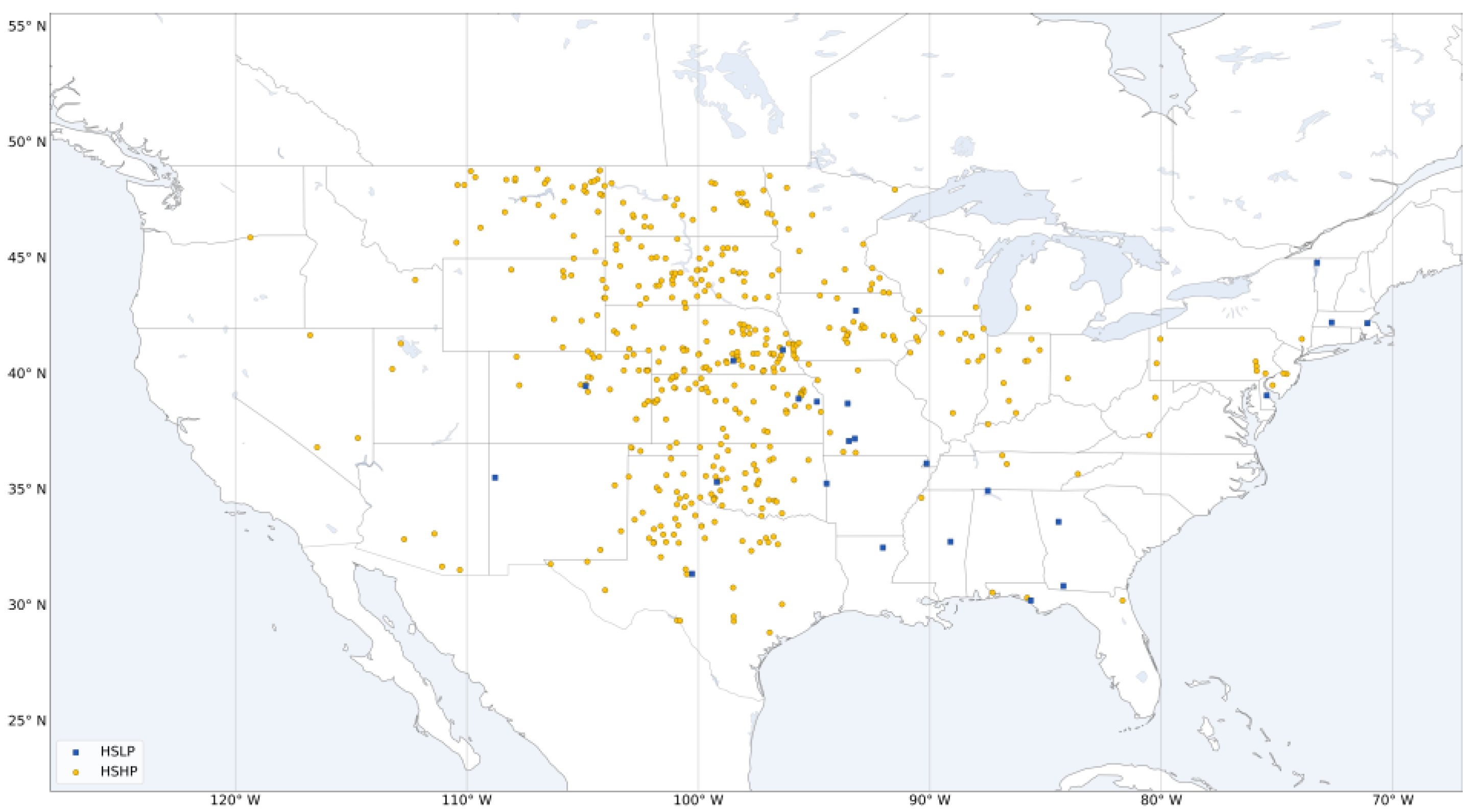
To find possible limitations or biases with the ML output, cases where high wind speeds were observed but the ML algorithm assigned low probabilities of severe wind (HSLP) and cases where low wind speeds were observed but high probabilities assigned by ML (LSHP) were further investigated. High speed was defined as a wind speed ≥ 65 knots, with a low speed defined as a wind speed < 50 kts. Since the classification threshold used during the training of the ML models in [12] was 0.5, low probability was defined as a GLM probability <0.5 and a high probability was defined as a GLM probability ≥0.5 for the present study. A comparison of GLM-assigned probabilities to measured wind speeds in SRs from 2018 to 2021 is shown in Figure 2. The threshold of 65 kts was used for high speeds since it is the value for thunderstorm winds to be considered significantly severe, and a low probability from the ML model in these cases implies a substantially different probability than what would be expected. Of the SRs evaluated, 9% met this criterion for high speed. Given the relatively small number of SRs that are input into the Storm Events Database with winds < 50 knots (only 1.4% in our sample), the criteria used for these analyses to represent low wind speeds was kept at <50 kts.

Both HSLP and LSHP events are compared to control cases or expected pairings of high speed—high probability (HSHP) and low speed—low probability (LSLP) cases, respectively. The wind speed and GLM probabilities are distinguished with the same bounds as the HSLP and LSHP cases, as shown in Figure 2. In total, there are 24 HSLP, 37 LSHP, 511 HSHP, and 45 LSLP reports. Comparatively fewer SRs fell into the LSHP and LSLP groups since most SRs are associated with winds at or above 50 knots, due to the verification guidelines applied to the Storm Events Database thunderstorm wind report database [24].

Statistical testing was conducted to compare the groups of HSLP cases to HSHP and LSHP to LSLP. Due to there being unequal sample sizes between groups and non-normally distributed mesoanalysis data, the Mann-Whitney U-Test was used to perform these evaluations [25]. Since 31 statistical tests were conducted, the Bonferroni Correction was used to decrease false positives [26]. This correction decreases the α value by dividing by the number of tests being conducted (31 in this case); therefore, significance with 95% confidence was determined with α ≤ 0.0016.

To compare convective morphologies and terrain types between the different types of reports to determine what role these differences might play, a random subset of events in the HSHP and LSLP sets was selected to match the much smaller number of HSLP and LSHP cases, respectively. Five sets of 24 random events were selected from the HSHP events, and 37 events from the LSLP events. The five sets of HSHP events were checked to ensure there were no duplicate reports. The 120 HSHP events were normalized to find the average number of events in each morphology per 24 events. For HSLP and HSHP cases, the focus of the analysis was on differences in convective morphology, while for the LSHP and LSLP cases, the focus was on the impact of terrain and the presence of a water body in the vicinity of the report.

The high-speed sets were organized into categories based on the convective mode. The categories used were isolated cells (IC), clusters of cells (CC), broken lines (BL), no stratiform lines (NS), trailing stratiform lines (TS), parallel stratiform lines (PS), leading stratiform lines (LS), bow echoes (BE), or non-linear (NL) as defined in [27]. IC, CC, and BL were considered cellular and NS, TS, PS, LS, and BE were linear. The nearest operational Doppler weather radar was used to determine the storm morphology with particular focus on the reflectivity and Doppler velocity products.

To further evaluate the reports deemed to be counterintuitive, we also looked to see if there were other measured SRs nearby. To be defined as “nearby”, a measured SR had to be within 0.144 degrees (~16 km) and had to have occurred within ±15 min of the misclassified SR. This criterion was chosen to capture measurements taken under similar environmental conditions and, ideally, from the same thunderstorm complex. The wind speeds and ML probabilities of nearby SRs were compared with those of the SRs whose probability values were counterintuitive.

To explore regional variations in the frequency of the counterintuitive events, boundaries were established with the central US falling between 105° W and 90° W and the eastern US being determined as east of 90° W. These regional bounds were chosen to roughly match geographic and climatological tendencies of storm reports [28]. The spatial distribution of reports for HSLP and LSHP events was compared to that for HSHP and LSLP, respectively. Further, these were compared to the regional distribution of the training set, where 14% occurred in the west, 60% occurred in the central US, and 26% occurred in the east.

The low-speed reports were broken down into categories based on where the report occurred: mountains/terrain shifts, coastlines, both, or none. The category for none was used for events that did not fit in one of the other categories. The event was within range of a mountain and/or terrain shift when there was a 100-m change in elevation relative to the report within 2 km or a 500-m change relative to the report within 10 km, with this criterion subjectively determined based on the authors’ experience relating terrain features to noticeable wind impacts. An event was identified as being coastal if it was within 10 km of an ocean or bordering a lake with its long axis larger than 10 km.

Model soundings were plotted using the 20- or 13-km RAP data at the closest model grid point to the SR location. The RAP was used in the creation of these plots since it forms the background analysis in the mesoanalysis dataset [21]. General patterns in sounding characteristics were used to draw conclusions based on documented sounding structure for primary drivers of severe wind, such as downbursts and microbursts.

4. Results

4.1. HSLP vs. HSHP

Bonferroni-adjusted p-values evaluated at the 95% significance level suggest differences between HSLP and HSHP cases in 15 of the 31 meteorological parameters. These parameters are listed in

Table 2. List of statistically significantly different mesoanalysis parameters for HSLP vs. HSHP cases. Bonferroni adjusted p-values and parameter means of each group are listed for each parameter.

Name	p-Value	HSLP Mean	HSHP Mean
Thermodynamic Parameters
SBCP (J kg−1)	0.0002	755.73	1650.53
MUCP (J kg−1)	0.0010	1384.99	2206.75
DNCP (J kg−1)	<<1	545.63	946.68
M1CP (J kg−1)	0.0006	898.36	1648.31
MUCN (J kg−1)	<<1	−7.61	−65.27
LR75 (°C km−1)	<<1	6.34	7.40
LR85 (°C km−1)	<<1	6.20	7.08
LPS4 (°C km−1)	<<1	0.05	0.04
SLCH (m)	0.0002	515.34	942.00
RH80 (%)	<<1	84.63	67.51
RH70 (%)	0.0002	78.50	62.32
3KRH (%)	<<1	83.66	64.87
RHLC (%)	<<1	89.42	71.25
Composite Parameters
QTRN (g kt kg−1)	<<1	34,065.91	103,944.93
EDCP (numeric)	0.0008	1.23	2.61

, along with their adjusted p-value and mean parameter values.

The mesoanalysis data for the SRs with low ML-assigned probabilities (HSLP) had meteorological parameters that were less favorable for severe convective wind than those for SRs with high ML-assigned probabilities (HSHP) (see Table 2). HSLP events had, on average, less convective available potential energy (CAPE; SBCP, MUCP, M1CP), less downdraft CAPE (DNCP), less convective inhibition (CIN; MUCN), less unstable lapse rates (LR75, LR85), lower lifted condensation level (LCL) heights (SLCH), increased relative humidity (RH80, RH70, 3KRH, RHLC), smaller values of storm relative moisture transport (QTRN), and smaller values of the Evans Derecho Composite Parameter (EDCP).

In general, the average parameter values of the HSLP SRs were less suggestive of environments capable of producing severe winds. Weaker instability, less unstable lapse rates, and increased relative humidity suggest less vigorous convection and convective organization, and less evaporative cooling, which lends to weaker cold pools. These results suggest that the low probability values assigned by the ML tool for the HSLP cases were reasonable from a meteorological perspective, focusing on the mesoscale environment present.

There were six HSLP reports with nearby measured SRs; three HSLP with one SR nearby, one HSLP with two SRs nearby, and one HSLP with four nearby. Information about nearby SRs to HSLP events is listed in

Table 3. Nearby measured SRs to HSLP reports. “HSLP Probability” represents the GLM probability for the HSLP report, “HSLP Speed” shows the measured gust of the HSLP report, “Number Nearby” represents the number of measured SRs nearby to the HSLP report, “Probability Nearby” is the array of probabilities nearby to the HSLP report, and “Speed Nearby” is the array of wind speeds nearby. The order in the arrays or probabilities corresponds to the order in the arrays of speeds.

Date	HSLP Probability	HSLP Speed	Number Nearby	Probability Nearby	Speed Nearby
13 April 2020	0.3065	69	2	[0.3181, 0.6320]	[56, 59]
6 June 2020	0.4262	70	1	[0.7422]	[63]
7 October 2020	0.4154	76	1	[0.2097]	[55]
10 April 2021	0.1632	65	1	[0.2762]	[51]
1 December 2018	0.1232	72	2	[0.0966, 0.3457]	[64, 56]
1 December 2018	0.2500	70	4	[0.0966, 0.3457, 0.2028, 0.1997]	[64, 56, 59, 59]

. When nearby SRs occurred, in general, they also had relatively high wind speeds and relatively low ML probabilities; however, the speeds and/or probabilities did not quite reach the thresholds to be considered HSLP in the present study. Since the criterion to be defined as “nearby” was within ±15 min and 0.144 degrees, the mesoanalysis output used for nearby points in the present evaluation was likely the same or only slightly shifted in time or space from the original HSLP report. The similar ML output between the HSLP cases and nearby SRs suggests that something within the broad-scale environment suggested a lower likelihood for the production of severe wind; however, something within the finer scale environment allowed for the development of strong winds.

The locations of HSLP events can be compared to HSHP events in Figure 3. For HSLP cases, 37.5% were in the east, 58.3% were in the central US, and 4.2% were in the west. On the contrary, for HSHP reports, 7.8% were in the east, 83.4% were in the central US, and 8.8% were in the west. A higher percentage of HSLP events occurred in the east compared to HSHP. This is an important difference to note due to the highly regional climatological occurrences of severe wind forcing, like wet and dry microbursts. Dry microbursts and environments categorized by “inverted-V” soundings are most common in the High Plains and the western US [29], while wet microbursts are most common in the eastern US and east of the High Plains.

Figure 4 shows an example of a sounding for one HSLP case (event id 764827), where the measured wind speed was 66 kts and the GLM probability of wind being severe was 0.3927. This sounding is shown since the wind and moisture profiles are relatively consistent with the other HSLP event soundings. This sounding is representative of soundings described by both [29,30] to be common with wet microbursts. The main difference between the HSLP profiles was in the strength of the dry air in the mid-layers. The most similar aspect of the cases was a lack of strong winds throughout the profile. Only three of the profiles showed speeds in any part of the profile greater than 30 kts. Most showed winds generally less than 10–15 kts from the surface to 500 mb. Environments with weaker shear (as would be the case with weak winds at all levels) were found by [29] to be more likely to produce short-lived pulse-like convection. Pairing the weak shear with the common trait of a dry layer above the moist layer in the sounding suggests that wet microbursts caused by pulse thunderstorms likely resulted in the very intense winds in these environments, and such environments may not result in high probabilities from the ML algorithm.

Considering convective morphologies, more IC, BL, NS, TS, PS and LS cases were noted in the HSLP set (

Table 4. Mean and standard deviation of convective modes in the HSHP set of cases, along with the total number of each morphology in the HSLP set.

Convective Morphology	HSHP Mean	HSHP Standard Deviation	HSLP Count
Isolated cells	1.8	0.40	3
Clusters of cells	3.6	1.36	1
Broken line	2.6	1.02	3
No stratiform	1.6	0.49	2
Trailing stratiform	6.0	1.26	9
Parallel stratiform	0.4	0.80	1
Leading stratiform	0.0	0.00	1
Bow echoes	4.6	0.49	2
Non-linear	3.4	1.02	2

). Of these, differences of greater than one standard deviation were noted for IC, NS, TS, PS, and LS modes. More CC, BE, and NL cases were noted in the HSHP set. All three morphologies saw differences of greater than one standard deviation.

Four of the 24 (16.7%) HSLP reports occurred in the immediate vicinity and at the same time as a tornado. None of the 120 HSHP reports occurred because of a tornado. To investigate if there were any signs of tornado-favorable environments in the mesoanalysis data, significance testing was conducted comparing the two groups (see

Table 5. List of mesoanalysis parameters statistically significantly (p < 0.05) different between tornadic vs. non-tornadic cases. Parameter means and p-values of each group are listed for each parameter.

Name	p-Value	Tornadic Mean	Non-Tornadic Mean
Thermodynamic
SBCP (J kg−1)	0.016	180.53	870.77
LR85 (°C km−1)	0.025	5.718	6.298
RH70 (%)	0.022	91.39	75.93
SLCH (m)	0.034	169.49	584.51
DNCP (J kg−1)	0.00016	229.29	608.90
Kinematic
VPMW (kt)	0.028	31.49	12.25
SRH3 (m2s−2)	0.013	439.29	198.69
VEIL (kt)	0.0056	36.64	13.95
Composite
XTRN (g kt kg−1)	0.039	436.95	275.56
EDCP (numeric)	0.045	0.561	1.362

). The difference between mesoanalysis parameters at the center of the domain for those four cases and the remaining 20 cases was found to be statistically significant (p < 0.05) for some thermodynamic (SBCP, LR85, RH70, SLCH, DNCP), kinematic (VPMW, SRH3, VEIL), and composite (XTRN, EDCP) parameters. Out of those 10, the downdraft CAPE and V component of the wind at the top of the effective inflow layer were found to also be significant at p < 0.01. The remaining 21 variables were found not to be statistically significant at p < 0.05. To determine the value of p, a two-tailed two-sample unequal variance t-test function was used. These results raise questions about whether winds related to a tornado may occasionally be incorrectly reported as severe thunderstorm winds in the SRs, since the ML algorithm does not diagnose particularly high probabilities for severe thunderstorm winds in these cases. It is also possible, however, that very small-scale damaging winds directly related to the tornado, but not a part of the tornado, occur in these cases, and such winds are not well-supported by the storm-scale environment resolved on the 40-km grid used for training of the ML algorithm.

4.2. LSHP vs. LSLP

A comparison of mesoanalysis parameters between LSHP and LSLP events (

Table 6. As with Table 2, but for LSHP vs. LSLP cases.

Name	p-Value	LSHP Mean	LSLP Mean
Thermodynamic Parameters
LR85 (°C km−1)	<<1	6.70	5.90
RH80 (%)	<<1	67.69	85.90
RH70 (%)	0.0012	65.39	79.22
3KRH (%)	<<1	64.09	78.02
RHLC (%)	0.0004	76.53	86.86
DNCP (J kg−1)	<<1	958.68	559.29

) found that of the 31 parameters, six were statistically significantly different between LSHP and LSLP cases. For the SRs with low wind speeds, SRs with high probabilities assigned by the ML algorithm (LSHP) occurred in environments with steeper lapse rates (LR85), less relative humidity (RH80, RH70, 3KRH, RHLC), and larger downdraft CAPE (DNCP) (see Table 6). These environmental parameters are suggestive of environments more likely to produce severe winds.

There were 3 LSHP reports with nearby measured SRs. Information about the nearby SRs is listed in

Table 7. As in Table 3, except for LSHP cases.

Date	LSHP Probability	LSHP Speed	Number Nearby	Probability Nearby	Speed Nearby
12 February 2019	0.5571	43	1	[0.2882]	[47]
28 March 2021	0.6647	41	1	[0.6724]	[50]
24 September 2021	0.8824	47	1	[0.6462]	[50]

. The comparison of the nearby SRs to LSHP reports is less straightforward than that for HSLP reports. Each of the 3 LSHP reports had only 1 SR nearby. The first LSHP event had a nearby SR with a wind speed of 47 knots and a probability of 0.2882, somewhat different from the LSHP event, which had a wind speed of 43 knots and a relatively high probability of 0.5571. Thus, the SR with a higher wind speed was assigned a lower probability than the SR with a lower wind speed. The nearby SR for the second LSHP case had a similar probability (0.6724) to that assigned to the LSHP report (0.66447). Despite these probabilities being similar, the LSHP event had a wind speed of 41 knots, but the nearby SR had a measured severe wind gust of 50 knots. The final LSHP report with a nearby SR followed a similar trend to the first LSHP report discussed above, where the nearby SR had a higher wind speed and lower probability than the LSHP event. For these LSHP events, the winds at nearby SRs, although sometimes severe, were only marginally so, complicating interpretation about why a generally favorable environment that led to high probabilities did not produce stronger winds.

The locations of LSHP and LSLP events are shown in Figure 5. Using the same regional constraints, 54.1% of LSHP events were in the east, 27.0% were in the central US, and 18.9% were in the west. For LSLP, 91% were in the east, 4.4% were in the central US, and 4.4% were in the west. It was found that many of the LSHP and LSLP events were located within the bounds of the county warning area served by the National Weather Service (NWS) office in Columbia, South Carolina. Of the 37 randomly selected LSLP events, 29 (78.4%) were found to happen in Columbia’s area of responsibility. The LSHP events had lower numbers of reports occurring within Columbia’s area at 13 out of 37 (35.1%). To account for the influence of this office in the reporting, event counts for terrain type were also found with this office excluded.

Many LSHP reports occur in complex terrain or near bodies of water, so it is possible that local influences prevented higher winds. While there are still some LSHP events that occur in the central US, where it has been shown that the GLM shows significant skill, many of the reports occur outside this region, in or near the Rocky Mountains in the west and the Appalachians in the east.

Of the 37 LSHP events, 10 occurred in regions of relatively complex terrain. The events in terrain were in California, Arizona, New York, Massachusetts, Vermont, and Georgia. In comparison, there was only one LSLP event that met the elevation change criteria to be defined as complex terrain. This event was in Virginia. Three events were classified as coastal in both the LSHP and LSLP groups. Two coastal LSHP events and one coastal LSLP event were found on Lake Murray in South Carolina. These were the only cases that met the coastal classification due to being near a large lake. The remaining coastal LSHP event and two coastal LSLP events were in Florida. No events in either LSLP or LSHP happened in areas in proximity to both coasts and terrain changes. Finally, 33 LSLP events and 24 LSHP events did not occur near a coast or terrain (see

Table 8. Comparison of the different terrain types for LSLP and LSHP cases, with (left two columns) and without (right two columns) events that occurred in NWS Columbia, SC’s county warning area.

Type	Including NWS Columbia, SC		Excluding NWS Columbia, SC
	LSLP Count	LSHP Count	LSLP Count	LSHP Count
Terrain	1	10	1	10
Coastal	3	3	2	1
Both	0	0	0	0
Neither	33	24	5	13

).

Due to the relatively small sample size of the LSHP events and variability in the soundings among these events, no general trends could be found from the sounding analysis. The lack of consistency among the soundings may be influenced at least partly by the large variability in the locations of the cases (see Figure 5).

5. Discussion and Conclusions

The ML tool created by [12] has been shown to have significant skill in diagnosing probabilities that a wind report was caused by wind ≥50 kts, with the GLM scoring a 0.9062 area under the receiver operating characteristic curve. In the present study, we investigated those relatively rare events where the ML tool diagnosed probabilities that seemed inconsistent with the measured winds associated with some SRs. This included events where ML-derived probabilities were low (high) for high (low) wind speed events from 2018 to 2021. Such an evaluation is important to learn limitations to the tool’s use and to better understand the full range of atmospheric conditions that can result in damaging thunderstorm winds or prevent their occurrence.

Despite having seemingly less conducive atmospheric conditions for producing severe wind, HSLP events did have measured wind speeds well above the severe criteria, with speeds ≥65 kts. HSLP events were shown to have smaller values of CAPE, less unstable midlevel lapse rates, and increased midlevel relative humidity compared to HSHP events. The comparison between the average mesoanalysis parameter values among these cases, along with an analysis of soundings, suggests that many HSLP events likely occur from wet microbursts. The regional distribution of HSLP events also agrees with this conclusion, as the events usually happen in the areas indicated in previous studies to experience more wet microbursts.

It is hypothesized that these SRs were assigned low probabilities due to the relative rarity of SRs from wet microbursts in the original training dataset. Since microbursts have a horizontal width of 4 km or less [31], the likelihood of one occurring at a measurement site is very limited. Ref. [32] found that to detect downbursts from weakly forced thunderstorms, a measurement network would have to have station spacing of 1.58 km or less. Given the average spacing of current networks, there is a 0.7% probability for a network to measure a wind gust ≥ 50 kt. Ref. [28] found that measured SRs most frequently occurred in the Great Plains and Midwest due to supercells and quasi-linear convective systems. Since only 26% of the data used in the training of the ML tool created by [12] occurred east of −90°, the conditions leading to wet microbursts may not be adequately represented in the full dataset.

To further understand the output of the ML tool in these unusual cases, SRs near HSLP reports were also examined. It was found that these nearby SRs were assigned probabilities by the ML tool that were generally similar to those of the HSLP reports, consistent with the fact that the reports were close in location and timing, and the same large-scale environment that was not particularly supportive of severe thunderstorm winds was present for all these reports. This supports the idea that there may be finer-scale features, like storm interactions, that result in localized higher wind speeds in these cases.

Individual cells are more likely to be a part of the HSLP group than the HSHP sets on average. Otherwise, broken lines, no stratiform, trailing stratiform, parallel stratiform, and leading stratiform lines were more common in the HSLP set. Only broken lines produced numbers for HSLP cases that were within one standard deviation of the HSHP average.

For the morphologies where the HSHP average count was higher than the HSLP count, the largest differences were present for clusters of cells and bow echoes. This indicates that the ML model is more consistent when predicting severe reports that originate from those. It is believed that the mesoanalysis better captures the environment for those morphologies. In the case of bow echoes, the type of environments that can produce a bow echo are usually much more favorable for significant severe gusts than those for other convective morphologies. The HSHP average was also found to be higher in the non-linear morphologies.

The four events caused by tornadoes had differences in 10 of the 31 weather parameters that were statistically significant with p < 0.05 and two others significantly different with p < 0.01 from the remainder of the HSLP cases. The two most significantly different were lower values of downdraft CAPE and higher speeds for the V component of the wind at the top of the effective inflow layer for the events where tornadoes were present. Higher values of downdraft CAPE indicate a higher potential for downdrafts. Downdrafts interfere with tornado development and growth by expanding the cold pool underneath the storm. A larger V component of the wind at the top of the effective inflow layer suggests stronger shear and increased storm-relative helicity (SRH), favoring tornadogenesis. SRH (surface to 3 km) was also found to be significantly different in these events, with p = 0.013.

SRs with a low wind speed but assigned high probabilities by the ML tool (LSHP events) were found to occur in environments where the meteorological parameters would promote severe wind. Compared to LSLP events, LSHP reports occurred with steeper LRs, drier mid-levels, and larger downdraft CAPE values. Two of the nearby SRs to LSHP reports did have marginally severe wind speeds (50 kts) and higher ML probabilities (>0.6) suggesting that the probabilities from the GLM were reasonable given the larger scale environment, and the lack of severe wind in the LSHP reports was an anomaly possibly related to storm-scale changes in the environment or individual thunderstorm structure, or perhaps reporting deficiencies.

The reason for the high number of LSLP and LSHP events in NWS Columbia, SC’s county warning area appears to result from a difference in reporting events to the Storm Events Database [33]. The national policy is to only submit a report with sub-severe winds if damage is associated with it or the wind measurement occurs in the immediate vicinity of the damage, and to mention that damage in the event narrative for the report. NWS Columbia, SC does not mention damage or other impacts in any of the 29 reports from them in the LSLP set or in any of the 13 reports from the LSHP set. These findings reveal one of the challenges when developing ML tools, the impact of problems in the data used for training. It can be difficult to find all possible problems that can negatively impact the skill of the ML tools. Fortunately, the sample size for this particular tool was large enough that overall performance was excellent [12], but the current findings suggest skill would likely have been improved further if additional quality control could have been performed on the training data.

Many of the LSHP events happened in complex terrain. These SRs had low wind speeds but were assigned high probabilities, consistent with environments conducive to thunderstorm wind. Given the impact complex terrain can have on atmospheric conditions, the mesoanalysis data used for training and testing of the ML tool may be of insufficient resolution to allow the tool to diagnose lower probabilities in these cases. Due to the relatively small sample size of measured SRs with speeds less than 50 kt and the impact of reporting differences, it is difficult to make broad conclusions about these cases, however.

The present work highlights the difficulties with forecasting severe wind, especially events categorized by weaker synoptic-scale forcing and complex terrain and geography. The output of the ML tool created by [12] was shown to be consistent with our understanding of atmospheric conditions favorable for severe thunderstorm winds, and likely its high level of skill comes from reports associated with well-organized convection, such as mesoscale convective systems and supercells. Given the relatively smaller number of measured severe thunderstorm wind events in the Eastern United States compared to the central part of the country, some situations that produce severe thunderstorm winds, such as wet microbursts, are likely not well-represented in the dataset.

The present study can be improved with the addition of more data, especially for the sub-severe cases. Since the Storm Events Database rarely includes events with measured sub-severe wind, additional cases should be collected using radar and surface observations of thunderstorms, as was performed in [12], as well as resampling methods. More detailed radar analysis could be performed on storms that resulted in SRs close to each other to better understand why winds may have varied greatly in the SRs, with a particular focus on the SRs where the winds did not seem to be consistent with the ML probabilities. This analysis could help answer questions about storm interactions, possibly intensifying winds in some cases beyond what would be expected from the larger-scale environment, or leading to interference, preventing winds from getting as strong as might be expected. [32] discusses the necessary station spacing required to detect severe wind produced by downbursts in weakly forced, pulse-like thunderstorms. With the mesoanalysis data having a 40 km grid spacing, further analysis into the impact of model grid spacing on the ML performance could be performed, perhaps by performing training and testing using convection-allowing model analyses such as the HRRR instead of the 40-km gridded mesoanalysis. While the present work analyzed feature relevance to improve confidence that the predictions of the algorithm [12] followed meteorological expectations, future work should expand on feature importance, especially on its impact on model performance, as laid out by [34].

References

1. Malone, T.F. Application of statistical methods in weather prediction. Proc. Natl. Acad. Sci. USA 1955, 41, 806–815. [Google Scholar] [CrossRef]
2. McGovern, A.; Lagerquist, R.; Gagne, D.J.; Jergensen, G.E.; Elmore, K.L.; Homeyer, C.R.; Smith, T. Making the black box more transparent: Understanding the physical implications of machine learning. Bull. Am. Meteor. Soc. 2019, 100, 2175–2199. [Google Scholar] [CrossRef]
3. Chase, R.J.; Harrison, D.R.; Burke, A.; Lackmann, G.M.; McGovern, A. A machine learning tutorial for operational meteorology. Part I: Traditional machine learning. Weather Forecast. 2022, 37, 1509–1529. [Google Scholar] [CrossRef]
4. Lagerquist, R.; McGovern, A.; Smith, T. Machine learning for real-time prediction of damaging straight-line convective wind. Weather Forecast. 2017, 32, 2175–2193. [Google Scholar] [CrossRef]
5. Steinkruger, D.; Markowski, P.; Young, G. An artificially intelligent system for the automated issuance of tornado warnings in simulated convective storms. Weather Forecast. 2020, 35, 1939–1965. [Google Scholar] [CrossRef]
6. Shield, S.A.; Houston, A.L. Diagnosing supercell environments: A machine learning approach. Weather Forecast. 2022, 37, 771–785. [Google Scholar] [CrossRef]
7. Cho, K.; Kim, Y. Improving streamflow prediction in the WRF-Hydro model with LSTM networks. J. Hydrol. 2022, 605, 127–297. [Google Scholar] [CrossRef]
8. Moosavi, A.; Rao, V.; Sandu, A. Machine learning based algorithms for uncertainty quantification in numerical weather prediction models. J. Comput. Sci. 2021, 50, 101–295. [Google Scholar] [CrossRef]
9. Sayeed, A.; Choi, Y.; Jung, J.; Lops, Y.; Eslami, E.; Salman, A.K. A deep convolutional neural network model for improving WRF Forecasts. IEEE Trans. Neural Netw. Learn. Syst. 2021, 34, 1–11. [Google Scholar] [CrossRef]
10. Haberlie, A.M.; Ashley, W.S. A method for identifying midlatitude mesoscale convective systems in radar mosaics. Part I: Segmentation and classification. J. Appl. Meteor. Climatol. 2018, 57, 1575–1598. [Google Scholar] [CrossRef]
11. Jergensen, G.E.; McGovern, A.; Lagerquist, R.; Smith, T. Classifying convective storms using machine learning. Weather Forecast. 2020, 35, 537–559. [Google Scholar] [CrossRef]
12. Tirone, E.; Pal, A.; Gallus, W.A.; Dutta, S.; Maitra, R.; Newman, J.; Weber, E.; Jirak, I. A machine learning approach to improve the usability of severe thunderstorm wind reports. Bull. Am. Meteor. Soc. 2024, 105, E623–E638. [Google Scholar] [CrossRef]
13. Smith, B.T.; Thompson, R.L.; Grams, J.S.; Broyles, C.; Brooks, H.E. Convective modes for significant severe thunderstorms in the contiguous United States. Part I: Storm classification and climatology. Weather Forecast. 2012, 27, 1114–1135. [Google Scholar] [CrossRef]
14. Kuchera, E.L.; Parker, M.D. Severe Convective Wind Environments. Weather Forecast. 2006, 21, 595–612. [Google Scholar] [CrossRef]
15. National Severe Storms Laboratory. Damaging Winds Types; NOAA National Severe Storms Laboratory: Norman, OK, USA, 2021.
16. Klingle, D.L.; Smith, D.R.; Wolfson, M.M. Gust front characteristics as detected by doppler radar. Mon. Weather Rev. 1987, 115, 905–918. [Google Scholar] [CrossRef]
17. Wakimoto, R.M. Convectively driven high wind events. In Severe Convective Storms; American Meteorological Society: Boston, MA, USA, 2001. [Google Scholar]
18. Trapp, R.J.; Wheatley, D.M.; Atkins, N.T.; Przybylinski, R.W.; Wolf, R. Buyer beware: Some words of caution on the use of severe wind reports in postevent assessment and research. Weather Forecast. 2006, 21, 408–415. [Google Scholar] [CrossRef]
19. Miller, P.W.; Black, A.W.; Williams, C.A.; Knox, J.A. Quantitative assessment of human wind speed overestimation. J. Appl. Meteor. Climatol. 2016, 55, 1009–1020. [Google Scholar] [CrossRef]
20. Edwards, R.; Allen, J.T.; Carbin, G.W. Reliability and climatological impacts of convective wind estimations. J. Appl. Meteor. Climatol. 2018, 57, 1825–1845. [Google Scholar] [CrossRef]
21. Bothwell, P.D.; Hart, J.; Thompson, R.L. An Integrated Three-Dimensional Objective Analysis Scheme. In Proceedings of the 21st Conference on Severe Local Storms, Norman, OK, USA, 13 August 2002; Available online: https://ams.confex.com/ams/SLS_WAF_NWP/techprogram/paper_47482.htm (accessed on 22 October 2019).
22. Li, J.; Heap, A.D. Spatial interpolation methods applied in the environmental sciences: A review. Environ. Modell. Softw. 2014, 53, 173–189. [Google Scholar] [CrossRef]
23. Benjamin, S.G.; Weygandt, S.S.; Brown, J.M.; Hu, M.; Alexander, C.R.; Smirnova, T.G.; Olson, J.B.; James, E.P.; Dowell, D.C.; Grell, G.A.; et al. A North American hourly assimilation and model forecast cycle: The Rapid Refresh. Mon. Weather Rev. 2016, 144, 1669–1694. [Google Scholar] [CrossRef]
24. NOAA, National Weather Service. National Weather Service Instruction 10-1605 July 26, 2021. Performance and Evaluation, NWSPD 10-16 Storm Data Preparation; NOAA, National Weather Service: Silver Spring, MD, USA, 2021.
25. Mann, H.B.; Whitney, D.R. On a test of whether one of two random variables is stochastically larger than the other. Ann. Math. Stat. 1947, 18, 50–60. [Google Scholar] [CrossRef]
26. Weisstein, E.W. Bonferroni Correction; Wolfram Research: Champaign, IL, USA, 2021; Available online: https://mathworld.wolfram.com/BonferroniCorrection.html (accessed on 13 September 2021).
27. Gallus, W.A., Jr.; Snook, N.A.; Johnson, E.V. Spring and Summer Severe Weather Reports over the Midwest as a Function of Convective Mode: A Preliminary Study. Weather Forecast. 2008, 23, 101–113. [Google Scholar] [CrossRef]
28. Smith, B.T.; Castellanos, T.E.; Winters, A.C.; Mead, C.M.; Dean, A.R.; Thompson, R.L. Measured severe convective wind climatology and associated convective modes of thunderstorms in the contiguous United States, 2003–2009. Weather Forecast. 2013, 28, 229–236. [Google Scholar] [CrossRef]
29. Johns, R.H.; Doswell, C.A. Severe local storms forecasting. Weather Forecast. 1992, 7, 588–612. [Google Scholar] [CrossRef]
30. Atkins, N.T.; Wakimoto, R.M. Wet microburst activity over the Southeastern United States: Implications for forecasting. Weather Forecast. 1991, 6, 470–482. [Google Scholar] [CrossRef]
31. Rose, M. Downbursts. Natl. Weather Dig. 1996, 21, 11–17. [Google Scholar]
32. Moore, A. Investigating the near-surface wind fields of downbursts using a series of high-resolution idealized simulations. Weather Forecast. 2024, 39, 1065–1086. [Google Scholar] [CrossRef]
33. Brooks, H.E. (NSSL, Norman, OK, USA). Personal communication, 2024.
34. Flora, M.L.; Potvin, C.K.; Skinner, P.S.; Handler, S.; McGovern, A. Using machine learning to generate storm-scale probabilistic guidance of severe weather hazards in the Warn-on-Forecast System. Mon. Weather Rev. 2021, 149, 1535–1557. [Google Scholar] [CrossRef]
Figure 1. Skill comparison among tested ML algorithms with (a) area under the receiver operating characteristic curve (AUC) for all six algorithms, and (b) subjective evaluation scores (scale of 1–10, with 10 being the best) for the top two objectively performing models (GBM, GLM) during the 2023 Spring Forecasting Experiment. Plots are calculated using data from [12], with objective scores in (b) being calculated using testing data from 2018 measured SRs.
Atmosphere 16 00881 g001
Figure 2. Wind speed vs. GLM probability for measured SRs from 2018 to 2021. Orange boxes represent groups distinguished by high wind speed—low GLM probability (HSLP) and low wind speed—high GLM probability (LSHP). Dashed black boxes represent the control groups of high wind speed—high GLM probability (HSHP) and low wind speed—low GLM probability (LSLP).
Atmosphere 16 00881 g002
Figure 3. Location of all the HSLP (blue squares) and HSHP (orange circles) storm reports.
Atmosphere 16 00881 g003
Figure 4. Example RAP sounding for a HSLP case. The green line represents dewpoint temperature and the red line represents the temperature. Surface-based CAPE is shaded in red, and surface-based CIN is shaded in blue.
Atmosphere 16 00881 g004
Figure 5. Location of all LSHP (blue squares) and LSLP (orange circles) storm reports.
Atmosphere 16 00881 g005