Performance Assessment of Low- and Medium-Cost PM_2.5 Sensors in Real-World Conditions in Central Europe

Abstract

In addition to the use of reference instruments, low-cost sensors (LCSs) are becoming increasingly popular for air quality monitoring both indoors and outdoors. These sensors provide real-time measurements of pollutants and facilitate better spatial and temporal coverage. However, these simpler devices are typically characterised by lower accuracy and precision and can be more sensitive to the environmental conditions than the reference instruments. It is therefore crucial to characterise the applicability and limitations of these instruments, for which a possible solution is their comparison with reference measurements in real-world conditions. To this end, a measurement campaign has been carried out to evaluate the PM_2.5 readings of several low- and medium-cost air quality instruments of different types and categories (IQAir AirVisual Pro, TSI DustTrak™ II Aerosol Monitor 8532, Xiaomi Mijia Air Detector, and Xiaomi Smartmi PM_2.5 Air Detector). A GRIMM EDM180 instrument was used as the reference. This campaign took place in Budapest, Hungary, from 12 November to 15 December 2020, during typically humid and foggy weather conditions, when the air pollution level was high due to the increased anthropogenic emissions, including wood burning for heating purposes. The results indicate that the individual sensors tracked the dynamics of PM_2.5 concentration changes well (in a linear fashion), but the readings deviated from the reference measurements to varying degrees. Even though the AirVisual sensors performed generally well (0.85 < R² < 0.93), the accuracy of the units showed inconsistency (13–93%) with typical overestimation, and their readings were significantly affected by elevated relative humidity levels and by temperature. Despite the overall overestimation of PM_2.5 by the Xiaomi sensors, they also exhibited strong correlation coefficients with the reference, with R² values of 0.88 and 0.94. TSI sensors exhibited slight underestimations with high explained variance (R² = 0.93–0.94) and good accuracy. The results indicated that despite the inherent bias, the low-cost sensors are capable of capturing the temporal variability of PM_2.5, thus providing relevant information. After simple and multiple linear regression-based correction, the low-cost sensors provided acceptable results. The results indicate that sensor data correction is a necessary prerequisite for the usability of the instruments. The ensemble method is a reasonable alternative for more accurate estimations of PM_2.5.

1. Introduction

One of the most alarming global public health concerns is air pollution [1,2]. Among the various pollutants, fine particulate matter (PM_2.5, that is, the common name for airborne particles with an aerodynamic diameter of 2.5 µm or smaller) is particularly significant due to its adverse effects on human health [3,4]. These particles are so small that they can penetrate deep into the lungs and even enter the bloodstream, posing a serious health risk to individuals, especially with prolonged exposure [5]. Research has linked PM_2.5 exposure to an increased risk of cardiovascular disease, particularly among the elderly [6,7]. Additionally, PM_2.5 was also associated with changes in respiratory symptoms and lung function [8]. Given the significant environmental concern and health impacts caused by aerosol particles, the monitoring and control of PM_2.5 levels are key to public health initiatives and pollution reduction strategies [9].

Regulatory air quality networks equipped with reference instruments (e.g., gravimetric or optical reference instruments) are essential for accurately assessing air pollution levels, providing credible information, and supporting environmental decision-making. However, reference instruments are costly to install and maintain, provide limited coverage, and thus do not necessarily reflect local variability in air pollution [10]. The limited number of stations scattered throughout a larger city may not give an accurate picture of the exact levels of pollutants in different parts of the city, as particulate matter may vary markedly depending on the emission sources and atmospheric conditions within the area of interest [11]. To address these shortcomings, as well as due to the increasing scientific and public demand, in recent years, the use of low-cost air quality instruments and their networking (including crowdsourcing) has grown rapidly worldwide [12,13,14,15,16]. According to the World Meteorological Organization [17], the use of low-cost sensors (LCSs) can contribute to the densification of the spatial monitoring of air quality, the identification of hotspots, rapid data access, and social engagement in the identification of environmental problems. These sensors offer real-time or near-real-time measurements for the pollutants through wireless connectivity modules and by offering meaningful measurements at the local level, which can support and expand the capabilities of the existing, official air monitoring networks [18].

Despite the obvious benefits of LCSs, it is important to note that these sensors’ precision, accuracy, stability, and lifetime are typically below those of the official reference sensors. One obvious reason for this fact is their measurement technique. Most of the LCSs evaluated in this study use optical methods (i.e., light scattering) for PM detection, which requires post-processing to convert particle number and size distributions to mass equivalents. This conversion introduces uncertainty that varies with aerosol composition and optical properties—a challenge that affects optical instruments across all price ranges, though reference instruments typically employ more sophisticated algorithms and calibration procedures. The uncertainty introduced can vary largely due to PM’s chemical composition and site-specific characteristics. Therefore, it is essential to carefully evaluate the sensor’s characteristics and limitations before using it in any practical application, e.g., exposure estimation [19,20]. Environmental conditions pose particular challenges for LCS performance: variations in relative humidity (RH) and air temperature (T) can introduce significant biases and uncertainties in their measurements, impacting their accuracy and reliability [21,22,23,24]. These environmental sensitivities may limit their suitability in certain deployment conditions without appropriate correction algorithms.

Several studies have analysed the reliability of different low-cost sensors in comparison with reference sensors and developed post-processing methods for data correction [6,25,26,27,28,29]. Variations in emission factors, aerosol chemical compositions, climatic conditions, and meteorological influences across different cities/regions can all impact the accuracy of low-cost sensors. Moreover, sensors of the same type often exhibit significant inter-unit variability. For these reasons, it is essential to conduct comparative measurements of the available low-cost sensors and reference instruments, taking into account local geographical and meteorological conditions, particularly in densely populated regions where such studies have not been previously conducted.

In Hungary, located in the densely populated Central Europe, along with many other natural and anthropogenic sources, domestic heating is one of the largest PM-emitting sectors during wintertime [30]. This includes burning wood and municipal waste in households [31], leading to high PM concentrations. In this sense, Hungary, and most importantly, its capital, Budapest, is an ideal environment to compare low-cost instruments with reference measurements while also enabling the collection of detailed meteorological data. As LCS evaluation studies are largely missing in Central Europe, we conducted a comparative measurement campaign at a monitoring site that is part of the Hungarian Air Quality Monitoring (HAQM) Network, operated by HungaroMet, in the suburban region of Budapest. This network provides hourly concentration data on key air pollutants, such as PM_2.5 (for details, see [32]) and others.

The main aim of the study is to present the setup of a comprehensive field evaluation campaign involving four different types of particulate matter sensors. A further goal is to assess the performance and accuracy of each sensor in real-world conditions against an accredited reference sensor. Additionally, we examine how various meteorological parameters and phenomena, such as humidity, temperature, or the occurrence of fog, influence the accuracy and reliability of the individual sensors. The novelty of the study is the inclusion of low-cost sensors that were not studied before, as well as the quantification of the intra-sensor variability.

Our results provide valuable insights into the accuracy of different price categories of sensors and the factors that influence their performance, which can be useful information for further environmental applications. The study supplements laboratory evaluations since the experiment was carried out in real-world conditions with high pollution in the densely populated Central European region.

2. Methodology

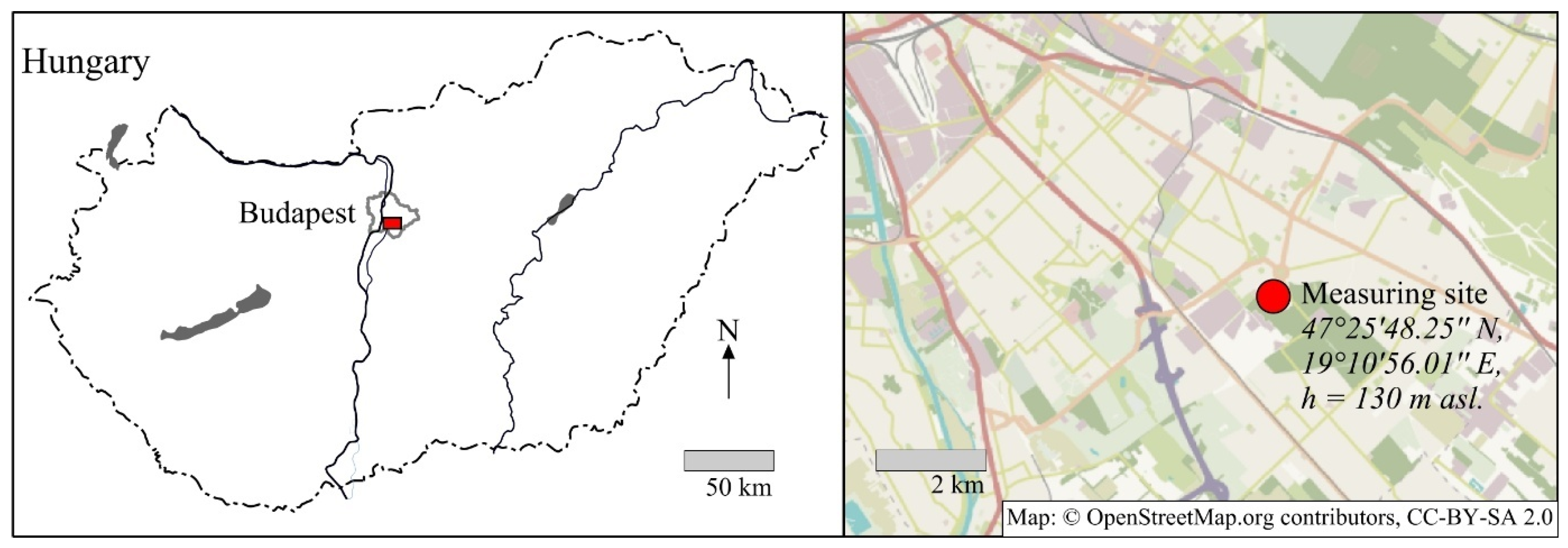
2.1. The Location and Timeframe of the Field Campaign

The performance of different PM_2.5 sensors was evaluated at the Gilice Square (Budapest, Hungary) urban background air quality monitoring station (47°25′48.25″ N, 19°10′56.01″ E, 130 m asl.). The station is located in the suburban southeastern part of Budapest (Figure 1), where the ambient air quality is mainly affected by local residential sources and traffic [33]. In Hungary, which is located in the Carpathian basin, high-air-pollution episodes frequently occur during autumn and winter due to the so-called “cold air pool” situation, which means inversion in a large part of the basin. In such situations, the background concentration can reach very high values, which also contributes to the local PM_2.5 concentration. Advection from upstream regions (densely populated downtown areas, industrial regions, etc.) also contributes to the actual PM_2.5 level.

The measurements were carried out between 12 November and 15 December 2020. The weather during the campaign was characterised by typically humid, cold conditions with foggy periods. Due to these weather conditions, domestic heating was also more intensive in the region. The measurement site serves as an official meteorological station of the Hungarian Meteorological Service (HungaroMet), providing automatic measurements of meteorological parameters at 10 min intervals throughout the campaign period.

2.2. Air Quality Sensors Used in the Experiment

During the measurement campaign, the performance of low- and medium-cost aerosol monitors was evaluated against a reference instrument, with a focus on PM_2.5. Based on the established literature and current market conditions, we define low-cost sensors as devices costing between USD 100 and USD 1000 (following [34]), while medium-cost sensors range from USD 1000 to USD 10,000 for complete systems, extending the classification framework of [35]. Low-cost PM2.5 sensors usually lack formal ISO/EN certification and show higher variability and humidity sensitivity, whereas medium-cost sensors are more likely to undergo standardised testing (e.g., ISO 16000-34 [36] and EN 12341 [37]) and include calibration and quality control methods aligned with international standards.

The tested devices included low-cost sensors (Xiaomi consumer devices, (Xiaomi, Inc., Beijing, China) and AirVisual Pro (IQAir, AG, Steinach, Switzerland) units) and a medium-cost TSI DustTrak II (TSI Incorporated, Shoreview, MN, USA) professional monitor. For consistency throughout this manuscript, all evaluated devices are collectively referred to as low-cost sensors (LCSs) when discussed together, keeping in mind that the DustTrak is in fact a medium-cost device.

Table 1. Technical data of the PM_2.5 sensors used for the comparisons. Six AirVisual sensors were used in the study, marked by #1–#6 in the table. Similarly, two DustTrak devices were used, marked by #1 and #2.

Device	AirVisual Pro (IQAir, AG, Steinach, Switzerland)	DustTrak II 8532 (TSI Inc., Shoreview, MN, USA)	Xiaomi Mijia Air Detector (Xiaomi, Inc., China)	Xiaomi Smartmi PM2.5 (Xiaomi, Inc., China)
Photo
Dimensions (mm) (H × W × D)	82 × 184 × 100	125 × 121 × 316	109 × 64 × 29.5	90 × 60 × 12
Weight (kg)	0.88	1.50	0.18	0.09
Measured parameters *	PM1, PM2.5, PM10, CO2, T, RH	PM1, PM2.5, PM4, PM10	PM2.5, TVOC, CO2, T, RH	PM2.5
Data storage	Internal memory, cloud storage via app	Internal memory	no storage	no storage
Sampling time interval	#1–#2: 15 min #3–#6: 3 min	3 min	3 min	3 min
Time period for operation (dd/mm)	#1–#2: 26/11–10/12 #3–#6: 12/11–15/12	#1: 12/11–20/11 #2: 12/11–26/11	8 separate days	8 separate days

* CO₂ is carbon dioxide, TVOC is the total volatile organic compound concentration, T is temperature, and RH is relative humidity.

provides an overview of the applied sensors, their temporal resolution, and the evaluation dates during the campaign. The sensors were tested in ambient air at 1.5 m height while housed in a self-made, rain-proof, ventilated box to protect against external influences (Figure 2). For various reasons, some of the individual air quality sensors were not operated for the entire period. Below, we provide technical data on the sensors and monitors. It should be noted that for some sensor types, multiple units were available, which enabled the analysis of inter-unit variability (i.e., differences between individual sensors of the same model type).

2.2.1. AirVisual Pro

Six AirVisual Pro indoor air quality monitors were used during the measuring campaign. AirVisual Pro is a widely used low-cost sensor manufactured by IQAir (IQAir, AG, Steinach, Switzerland) [4,38], which detects and records PM_2.5, PM₁₀, carbon dioxide, and some environmental variables (such as temperature (T) and relative humidity (RH)). PM concentration is determined by a light-scattering (optical) particle counter. Of the available sensors, two older, first-generation devices (manufactured before 2017) had a time resolution of 15 min, while the newer devices allowed for a sampling time of 3 min (better resolution was feasible, but it was not used for comparability with the first-generation sensors). The instruments record the data in their internal memory, which can be downloaded through Wi-Fi.

2.2.2. TSI DustTrak Aerosol Monitor

During the measurements, two TSI DustTrak II 8532 handheld aerosol monitors (professional grade) were also operated and were manufactured by TSI (TSI Incorporated, Shoreview, MN, USA). DustTrak monitors are also widely used for the determination of the aerosol mass concentration [39,40], even as reference instruments [41]. The DustTrak II 8532 device is a light-scattering laser photometer that uses impactors to measure PM₁, PM_2.5, PM₄, and PM₁₀ separately. Our study only used the 2.5 μm impactor for the measurements. Data were recorded with a 3 min time resolution, using the ambient calibration factor set in the instrument for outdoor environment conditions (with a photometer calibration factor (PCF) of 0.38). One unit was used for only 9 days due to technical problems, while the second unit performed measurements lasting for 2 weeks.

2.2.3. Xiaomi Sensors

Two types of compact, low-cost Xiaomi air quality sensors were also evaluated during the campaign. The first one, Xiaomi Mijia Air Detectors (Xiaomi Corporation, Beijing, China), is a small air quality monitor equipped with sensors for PM_2.5, CO₂, total volatile organic compounds (TVOCs), temperature, and relative humidity. Aerosol particles are measured using a built-in laser-based optical sensor. The second device was a Xiaomi Smartmi PM_2.5 Air Detector (Xiaomi Corporation, Beijing, China)—the most affordable of all devices included in the study. It displays real-time PM_2.5 concentrations and an air quality index on its screen. Xiaomi Smartmi (Xiaomi Corporation, Beijing, China) is also an optical sensor, using a laser-based particle counter. As these two devices do not have internal memory to support data storage, the measurements were manually recorded by reading the displays every 3 min over several hours across an 8-day period. To the best of the authors’ knowledge, these devices were not evaluated against reference instruments, which is one of the novelties of the present study.

2.3. The Reference Measuring Instrument

During the measurement campaign, hourly data obtained from a co-located GRIMM EDM 180, an approved reference-grade dust monitor, were also available (manufactured by GRIMM Aerosol Technik GmbH & Co. KG, Ainring, Germany). GRIMM EDM 180 utilises an optical light-scattering sensor to determine the mass concentration of PM₁, PM_2.5, and PM₁₀ as well as particle numbers within 31-size channels. It is capable of monitoring real-time particulate matter within a size range of 0.25 to 32 μm. GRIMM EDM 180 is also equipped with a Dehumidification System (Dryer) (GRIMM Aerosol Technik GmbH & Co. KG, Ainring, Germany) to reduce the relative humidity above 70%. GRIMM EDM 180 is widely used for reference measurements in air quality monitoring due to its high accuracy and reliability. The GRIMM equipment was located at a distance of about 10 m from the ventilated box that contained the LCSs, with air intake at a height of 4 m.

2.4. Data Processing and Statistical Analysis

The measurements from all LCSs were compared with the GRIMM reference data using traditional statistical analysis. All data were averaged to a 1 h time resolution to harmonise the temporal resolution of different instrumentation. The performance of the sensors was evaluated using several sensor accuracy metrics recommended by the U.S. Environmental Protection Agency (EPA) [42]. Simple linear regression (SLR) was used to assess the relationship between the hourly average concentration value (x) measured by the LCSs and those reported by the reference instrument. The results of the regression can be used to adjust the LCS data during post-processing:

$$\widehat{y}={\beta }_0+{\beta }_{1}x,$$

(1)

where $\widehat{y}$ is the predicted value of the sensor assuming a linear relationship, and the slope (β₁) and the intercept (β₀) are calculated by the regression. The coefficient of determination (R²) was also calculated to evaluate the agreement between the sensor data and the reference measurements.

Root Mean Square Error (RMSE), Mean Absolute Error (MAE) and Mean Bias Error (MBE) for each sensor were also calculated:

$$RMSE=\sqrt{{{\displaystyle \sum }}_{i=1}^n{\displaystyle \frac{{\left(x_i-y_i\right)}^2}{n}}},$$

(2)

$$MAE={\displaystyle \frac{{{\displaystyle \sum }}_{i=1}^n\left|x_i-y_i\right|}{n}},$$

(3)

$$MBE={\displaystyle \frac{{{\displaystyle \sum }}_{i=1}^n\left(x_i-y_i\right)}{n}} ,$$

(4)

where n is the number of data points, and x_i and y_i are the 1 h average concentrations at the i-th time step of the sensor data and reference instrument, respectively.

The accuracy (%) of low-cost sensors [43] is a measure of the closeness between the measured values of the sensors and the reference value. In this context, the accuracy can be calculated according to the following equation:

$$A=100-{\displaystyle \frac{\left|\overline{X}-\overline{Y}\right|}{\overline{Y}}}\ast 100,$$

(5)

where $\overline{X }$ is the average concentration measured by the sensors during the testing period and $\overline{Y }$ is the average concentration measured by the reference sensor during the same testing period. Low accuracy does not necessarily mean low performance, since bias is a typical feature of the LCSs. If the R² is high, the readings can be considered as applicable after correction.

Multiple linear regression (MLR) is an extension of SLR that integrates several independent variables, allowing for a more precise adjustment of low-cost sensor data. This technique is valuable for assessing the impacts of environmental factors such as temperature (T) and relative humidity (RH). MLR was calculated using the following general equation [44]:

$$\widehat{y}={\beta }_0+{\beta }_{1}x+{\beta }_{2}T+{\beta }_{3}RH,$$

(6)

where β₀, β₁, β₂, and β₃ are the regression coefficients.

Some PM_2.5 sensors (such as the AirVisual Pro) are equipped with integrated temperature and relative humidity sensors. However, they cannot be considered representative of the environmental conditions. Therefore, it is recommended to use reliable external meteorological data sources [45]. In this study, meteorological data were obtained from the meteorological station of the HungaroMet to also support such analysis for sensors without built-in temperature and humidity sensors.

3. Results

3.1. Meteorological Conditions During the Measurement Campaign

During the measurement campaign, typical late autumn weather conditions prevailed over Hungary (Figure 3). The weather was calm and humid at the beginning of the period. On 21 November, a cold air mass of Arctic origin arrived behind a strong cold front, and then the high-pressure area strengthened again. The overcast conditions persisted during these days, with daily temperatures consistently below the long-term average. In the last days of the month, a cyclonic cold front caused cooler-than-average weather. Then, from 3 December, a Mediterranean cyclone brought increasingly milder air masses and increased precipitation. The meteorological parameters, including temperature, precipitation, relative humidity, visibility, wind speed, and incoming solar radiation, were obtained for the entire period of the study from the official weather station of HungaroMet. Figure 3 presents the hourly meteorological data during the campaign.

In the campaign’s timeframe, the hourly temperature values varied between −4.6 and 13.3 °C. The cold front in late November led to a cooler-than-average beginning of December, with daily average temperatures 3–4 °C below the long-term average. The relative humidity varied from 28 to 100%, but low values occurred only rarely. Low visibility (less than 1000 m, indicating fog) occurred on a few days. There was only a little rainfall in the first half of the period and slightly more in the second half, although it occurred on only a few days overall. The total precipitation for the period was 22.7 mm. The wind was generally light with a slight increase in the second part of the campaign. The sea level pressure was high (>1020 hPa) in the first half of the period, then decreased later in the campaign. The temporal pattern of radiation reflects that the period was predominantly cloudy.

3.2. Comparison of Raw Data and Reference PM_2.5 Measurements

Figure 4 shows the complete time series for the campaign based on data from the LCSs and the reference instrument. The figure demonstrates the overall co-variation in the results but also highlights the biases in the data and the intra-sensor variability of the AirVisual devices.

Figure 5 shows the relationship between the LCS readings and the reference GRIMM data for all sensors, separately (green colour). The results indicate that the relationship between the reference sensor and the LCSs was typically linear. The slopes of the linear regression for all AirVisual Pro units and Xiaomi sensors are below 1, implying an overall tendency for overestimation of the reference PM_2.5. DustTrak II sensors’ slope is 1.02 for one TSI unit and 0.97 for the second unit, indicating unbiased observation.

Table 2. Summary of the statistics of sensors’ performance against the reference GRIMM device. N is the number of data pairs used to calculate the statistics.

Sensor	N	Slope	Intercept	R2	RMSE	MAE	MBE	Accuracy
					(µg/m3)	(µg/m3)	(µg/m3)	(%)
AirVisual 1	337	0.60	3.35	0.93	9.34	7.24	7.21	62.74
AirVisual 2	337	0.82	4.57	0.93	3.22	2.69	−1.43	92.56
AirVisual 3	633	0.49	3.29	0.88	17.22	14.06	14.03	30.60
AirVisual 4	633	0.62	3.32	0.86	9.66	7.28	7.01	65.34
AirVisual 5	633	0.59	3.00	0.85	11.52	9.15	8.90	55.94
AirVisual 6	633	0.48	2.05	0.92	20.46	17.55	17.55	13.17
TSI 1	83	0.97	6.21	0.94	6.30	5.71	−5.66	79.08
TSI 2	177	1.02	4.77	0.93	6.16	5.37	−5.21	79.43
Xiaomi Mijia	23	0.46	1.21	0.89	18.87	17.50	17.50	−0.81
Xiaomi Smartmi	23	0.56	−0.35	0.94	14.78	13.97	13.97	19.54

summarises the statistical results from the evaluations of the hourly average PM_2.5 concentrations measured by various sensors, as compared with the GRIMM reference monitor. The number of hourly data points (N) between each PM_2.5 sensor (AirVisual and TSI DustTrak) and the GRIMM monitor ranged between 83 and 633. In contrast, Xiaomi’s sensors had significantly fewer data points (only 23) due to their inability to automatically log measurement data.

Based on the statistical analysis, the TSI DustTrak monitors demonstrated the highest correlation with the reference data, generally outperforming the AirVisual Pro units. However, some AirVisual Pro sensors also showed high correlation, with R² values around 0.93. Notably, the Xiaomi Smartmi device exhibited a surprisingly strong correlation (R² = 0.94), while the Xiaomi Mijia sensor showed a slightly lower correlation (R² = 0.89). It is important to note that these latter values are based on a limited number of data points.

RMSE for AirVisual Pro exceeded 9 µg/m³, except for the AirVisual #2 unit (3.22 µg/m³). Both DustTrak units fulfil the U.S. EPA RMSE metric with values below 7 µg/m³. In contrast, the Xiaomi sensors exhibited high RMSE values. The best statistical parameters were obtained with one AirVisual sensor (#2) and two TSI sensors. In addition, the two TSI sensors gave very similar results.

Despite the similar correlation coefficients (R²), the slope and intercept values varied significantly between sensors, even among those of the same model, such as the AirVisual Pro.

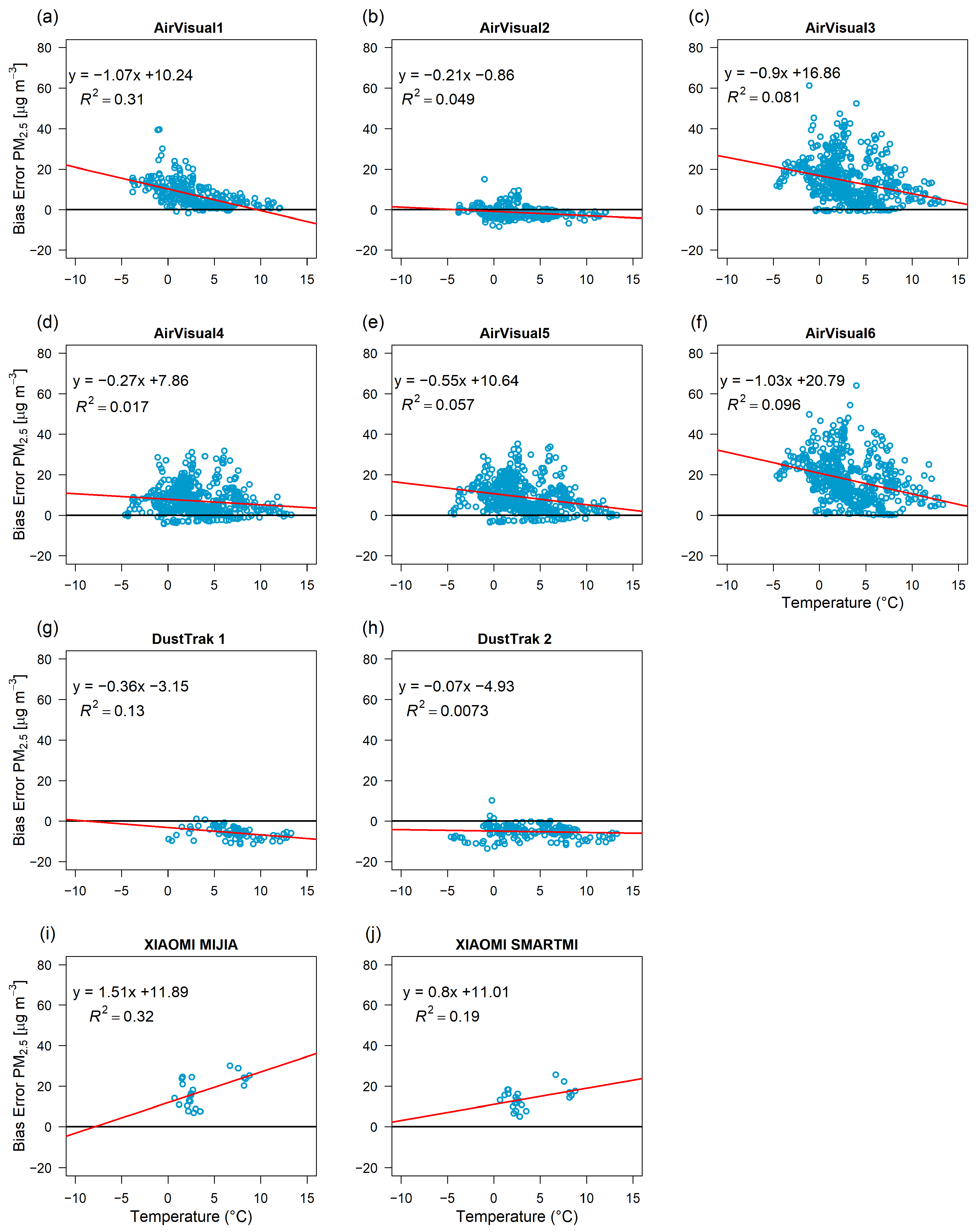
3.3. Impacts of Atmospheric Conditions on the Accuracy of the Sensors

To assess the impact of relative humidity on PM_2.5 measurements from low-cost sensors, hourly measurement error (i.e., the difference between sensor readings and those from the GRIMM reference monitor, in µg/m³) was plotted against hourly average relative humidity for six AirVisual Pro sensors and two TSI DustTrak sensors. As shown in Figure 6, at RH levels below 60%, no significant influence on sensor performance is observed. However, at higher humidity levels (RH ≥ 60%), errors increase, indicating an effect of RH on PM_2.5. The TSI DustTrak sensors show negligible sensitivity to humidity, with a tendency toward negative error (slight underestimation). The results also show that the error of the TSI DustTrak sensor is relatively unaffected by an increase in relative humidity. In contrast, the error of the AirVisual Pro sensors increases with increasing relative humidity. At higher humidity levels, the error shows an increasingly broad spectrum, suggesting that other external factors may also influence the variation. Interestingly, in the case of the Xiaomi sensors, the effect has the opposite direction compared to the AirVisual devices.

The influence of temperature on sensor performance was also examined by plotting hourly PM_2.5 measurement errors against ambient temperature (Figure 7). The red line in the plots represents the linear regression fit, illustrating the relationship between measurement error and temperature. Notably, all AirVisual Pro sensors exhibited a positive error (overestimation), with values increasing from 0 µg/m³ to approximately 40 µg/m³. The error decreased with increasing temperature. This trend is consistent across all AirVisual Pro units, except for Unit 2, where temperature appears to have a negligible effect. In contrast, the TSI DustTrak sensors show a negative error, with no significant correlation between temperature and sensor performance. In case of the Xiaomi sensors, the effect is, again, the opposite of the one observed with the AirVisual sensors, meaning a larger bias with increasing temperature.

3.4. Correction of the LCS Data

Two different methods were tested to adjust the LCS data to improve its accuracy. The first method uses the simple linear relationship between LCS data and the GRIMM data (Table 2) that was set according to the comparison presented in Figure 5.

The second method used the LCS data, plus T and RH, to construct a multiple linear regression-based equation (Equation (6)) for post-processing (or correction) of the original data per instrument (note that we do not call it calibration as the factory calibration remains unchanged).

Figure 5 shows these corrected data for all sensors (red and blue colours corrected by SLR and MLR, respectively).

Table 3. Summary of the statistics for the corrected data using simple linear regression. N: number of 1 h data points for linear regression.

Sensor	N	R2	RMSE	MAE	MBE	Accuracy
			(µg/m3)	(µg/m3)	(µg/m3)	(%)
AirVisual 1	337	0.93	2.28	1.47	−0.07	99.65
AirVisual 2	337	0.93	2.28	1.81	−0.09	99.51
AirVisual 3	633	0.88	3.39	2.42	−0.14	99.27
AirVisual 4	633	0.86	3.67	2.59	−0.02	99.90
AirVisual 5	633	0.85	3.78	2.66	−0.03	99.83
AirVisual 6	633	0.92	2.72	1.93	−0.03	99.81
TSI 1	83	0.94	2.75	2.21	−0.10	99.62
TSI 2	177	0.93	3.26	2.56	−0.04	99.82
Xiaomi Mijia	23	0.89	2.09	1.41	−0.11	99.34
Xiaomi Smartmi	23	0.94	1.47	1.16	−0.16	99.04

and

Table 4. Summary of the statistics for the corrected data using multiple linear regression based on RH and T. β₀: intercept; β₁: sensor PM_2.5 coefficient; β₂: RH coefficient; and β₃: T coefficient (see Equation (6)). N is the number of 1 h data points.

Sensor	N	β0	β1	β2	β3	R2	RMSE	MAE	MBE	Accuracy
							(µg/m3)	(µg/m3)	(µg/m3)	(%)
AirVisual 1	337	12.95	0.59 ***	−0.10 ***	−0.14 **	0.94	2.13	1.33	−0.01	99.94
AirVisual 2	337	13.04	0.79 ***	−0.07 ***	−0.27 ***	0.94	2.29	1.79	0.85	95.57
AirVisual 3	633	15.64	0.50 ***	−0.13 ***	−0.27 ***	0.90	3.07	2.11	0.12	99.36
AirVisual 4	633	18.15	0.63 ***	−0.15 ***	−0.44 ***	0.89	3.21	2.19	0.35	98.25
AirVisual 5	633	17.53	0.61 ***	−0.16 ***	−0.30 ***	0.88	3.37	2.30	−0.10	99.49
AirVisual 6	633	13.70	0.49 ***	−0.12 ***	−0.23 ***	0.94	2.42	1.68	0.58	97.08
TSI 1	83	19.18	1.03 ***	−0.15 **	−0.04	0.96	2.39	1.95	0.26	99.03
TSI 2	177	10.74	1.13 ***	−0.10 ***	0.10	0.94	2.97	2.33	0.03	99.87
Xiaomi Mijia	23	16.93	0.45 ***	−0.15 **	−0.39 **	0.95	1.39	1.14	0.30	98.26
Xiaomi Smartmi	23	13.18	0.53 ***	−0.13 **	−0.16	0.97	1.01	0.64	0.12	99.29

Significance: * p < 0.05 (did not occur in this data set), ** p < 0.01, and *** p < 0.001.

summarise the error metrics for the corrected PM_2.5 data by the two methods. The R² values shown in Table 2 did not change as the correction made a linear adjustment per data point.

Comparing the data of Table 4 with the statistical results presented in Table 3, it is clear that in the case of multiple linear regression, i.e., when environmental factors (RH and T) are considered, the error statistics show better performance in most cases.

In general, both methods improved accuracy (RMSE reduction by 50–80%), with MLR outperforming SLR for most sensors (e.g., Xiaomi Smartmi RMSE dropped from 14.78 to 1.01 µg/m³). TSI devices are already less affected by RH, showing minimal improvement, while Xiaomi sensors experienced considerable improvements. After SLR and MLR correction, the accuracy varied from 99.04% to 99.90% and from 97.08% to 99.94%, respectively (Table 3 and Table 4).

3.5. Ensemble Approach

Given the opportunity to use six different AirVisual sensors (with different firmware), an attempt was made to create a simple LCS ensemble for the corrected PM_2.5. This approach means that, contrary to individual accuracy testing, the aggregated values (mean and median PM_2.5) of six sensors were calculated, which were then used as a basis of comparison. This was carried out for the time period when all devices were running simultaneously, and the GRIMM dataset was also available. For each AirVisual Pro, the node-specific correction equations were used (Table 2 and Table 4), using SLR and MLR methods as well.

Table 5. Performance statistics for the individual AirVisual Pro devices and the ensemble mean (E. mean) and ensemble median (E. median) calculated from the data of the six sensors. The corrected data were calculated using both SLR and MLR. The green colour indicates the two best statistical indicators per metric.

	SLR				MLR
	RMSE	MBE	MAE	Accuracy	RMSE	MBE	MAE	Accuracy
	(µg/m3)	(µg/m3)	(µg/m3)	(%)	(µg/m3)	(µg/m3)	(µg/m3)	(%)
AirVisual1	2.28	−0.07	1.48	99.65	2.13	−0.01	1.34	99.94
AirVisual2	2.66	−0.02	2.05	99.92	2.29	0.50	1.57	97.39
AirVisual3	2.77	0.06	1.97	99.71	2.55	0.42	1.67	97.81
AirVisual4	2.28	−0.09	1.81	99.52	2.29	0.86	1.80	95.58
AirVisual5	2.56	0.19	1.99	99.04	2.29	0.22	1.64	98.88
AirVisual6	1.91	0.14	1.41	99.29	1.91	0.84	1.26	95.65
E. mean	2.13	0.03	1.67	99.82	1.90	0.47	1.37	97.56
E. median	2.42	0.02	1.89	99.59	2.29	0.46	1.61	97.60

shows the statistical evaluation of the results for the ensemble mean and ensemble median, and for the individual sensors, since the period used here is different from the one represented by Table 3 and Table 4. The table indicates that the ensemble mean outperforms the median (exceptions include MBE for SLR). Comparing the sensor-specific error metrics, the ensemble mean has some merits, and in one case, the best performance is associated with the ensemble mean (RMSE for MLR). Considering SLR, the ensemble mean outperforms five sensors for RMSE, five for MBE, four for MAE, and five for accuracy. In the case of MLR, the ensemble performs better than all six sensors for RMSE, three sensors for MBE, four sensors for MAE, and two sensors for accuracy. The results indicate that ensemble averaging of LCSs can provide improved performance with practical implications.

4. Discussion

4.1. Evaluation of LCS Performance

In this study, low- and medium-cost sensors were evaluated against a GRIMM reference instrument. The novelty of the study is the inclusion of sensors that have not been evaluated yet, according to the authors’ knowledge. These sensors have no internal memory, so the data is not recorded; thus, their evaluation is challenging, especially in outdoor conditions. We used manual registration to overcome this limitation.

One significant drawback of the LCSs is that, due to their inexpensive production, quality control in manufacturing varies considerably between manufacturers, resulting in substantial inter-unit variability. While some devices receive factory calibration, this is often insufficient for specific deployment environments. Furthermore, ageing and degradation play an important role [46], meaning that differences in usage profiles can cause substantial variation even among devices of the same type. Moreover, although the measurement methodology of different sensor brands is similar, the internal data processing methods (e.g., applied corrections) are usually unknown to the user and likely differ, leading to varied responses in diverse environments.

This variation indicates that while low-cost sensors may effectively capture the temporal patterns and relative changes in PM_2.5 concentrations, they often differ in their absolute accuracy. These discrepancies highlight the need for individual calibration or validation of each sensor prior to deployment.

Table 6 shows error statistics from the scientific literature focusing on LCS intercomparison with some reference instruments. Here, we focus exclusively on sensors (or similar types) that were also used in our study. It should be noted that the Xiaomi sensor included in the table most likely differs from those we used, as the dimensions reported by Li et al. (2020) [47] were different from those listed in Table 1. We did not find studies that evaluated the Xiaomi devices that we used.

The performance of identical types of low-cost sensors can vary significantly depending on the measurement environment, the reference instrument, and the measurement time scale. The frequently used AirVisual Pro low-cost sensor was tested in various geographical locations (USA, Switzerland, and Portugal), in both indoor and outdoor environments. The R² values vary widely (0.30–0.98), indicating that sensor performance strongly depends on environmental conditions, measurement time intervals, and the type of reference instrument. For example, ref. [26] observed moderate performance for 1 h outdoor sampling (R² = 0.69–0.72), while ref. [4] reported high accuracy for short (1 min) indoor measurements (R² = 0.89–0.90).

The TSI DustTrak series is also a popular instrument in use and is typically operated with a 2–10 min outdoor sampling resolution. The results reported by Li et al. (2019) [48] showed a large range of explained variance (R² = 0.36–0.97), reflecting the impact of seasonal and temporal variability. The study by Javed & Guo (2021) [49] indicated significantly higher performance (R² = 0.90), although the RMSE value (9.50) suggests the presence of considerable measurement errors.

Interestingly, the Xiaomi Mi PM_2.5 detector performed best in indoor environments (R² = 0.96–0.99), outperforming several other LCS devices. This suggests that simpler, commercially available sensors can also perform well under appropriate conditions.

The study by Sá et al. (2024) [50], also conducted in an indoor setting, shows a wide range of results (e.g., RMSE: 20.3–1.69 × 10³), but the extremely high RMSE/MAE/MBE values were caused by malfunctions in the study’s AirVisual sensors. This raises concerns about variability between individual sensors and potential calibration issues.

Table S1 in the Supplementary Materials shows the results of the statistical evaluation of other commercial LCSs in field conditions. The results show similar performance to the commercial devices used in our study.

Table 6. Studies focusing on the evaluation of some of the sensor types that were used in this study. N/A: not available.

Sensors	Geographical Location	Sampling Area and Time	Reference Instruments	Performance Indices	Reference
AirVisual Pro (3 units)	Riverside, CA/USA	Outdoor, 1 h	Met One BAM 1020 (Met One Instruments, Inc., Grants Pass, OR, USA)	R2: 0.69–0.72 RMSE: 5.8–7.3 MBE: 0.2–3.4 MAE: 4.4–5.3 Slope: 1.15–1.31 Intercept: −2.42(–)–1.97	Feenstra et al. (2019) [26]
AirVisual Pro (2 units)	Baltimore, MD/USA	Indoor, 1 min	Thermo Scientific pDR-1200 (ThermoFisher Scientific Inc. Waltham, MA, USA)	Accuracy: 86% RMSE: 0.59–0.64 R2: 0.89–0.90 MBE (%): 3.45–4.26	Zamora et al. (2020) [4]
AirVisual Pro (1 unit)	N/A	Indoor, 1 min	GRIMM 11C (GRIMM Technologies, Inc., GA, USA) TSI SidePak AM530 (TSI Inc., Shoreview, MN, USA)	R2: 0.90–0.95 R2: 0.88–0.96	Li et al. (2020) [47]
AirVisual Pro (3 units)	New Jersey, USA	Indoor, 5 min	TSI DustTrak DRX Model 8534 (TSI Inc., Shoreview, MN, USA)	R2: 0.30–0.98 Slope: 0.01–1.02 Intercept: −1.57–4.49	He et al. (2020) [38]
AirVisual Pro (1 unit)	Fribourg, Switzerland	Indoor, 5 min	GRIMM Model 1371, Aerosol Technik (miniWRAS). (GRIMM Aerosol Technik GmbH & Co. KG, Ainring, Germany)	r: 0.53–0.99	Demanega et al. (2021) [51]
AirVisual Pro	Porto, Northern Portugal	Indoor	TSI DustTrak DRX Model 8534 (TSI Inc., Shoreview, MN, USA)	R2: 0.60–0.88 RMSE: 20.3–1.69 × 103 MBE: −1.61 × 103–14.3 MAE: 18.8–1.62 × 103	Sá et al. (2024) [50]
TSI DustTrak 8520 (PM10)	Delaware, USA	Indoor, 10 min	Thermo Scientific TEOM 1405-DF (ThermoFisher Scientific Inc., Waltham, MA, USA)	R2: 0.85–0.92	Yang et al. (2018) [52]
TSI DustTrak 8530 (2 units, diff. seasons)	Hong Kong/China	Outdoor, 10 min	Thermo Scientific Model 5030 (ThermoFisher Scientific, Waltham, MA, USA) SHARP 5030, (Thermo Scientific Inc., MA, USA)	R2: 0.36–0.97	Li et al. (2019) [48]
TSI DustTrak 8530 (1 unit)	Hong Kong/China	Outdoor, 10 min	Thermo Scientific TEOM 1405-D (ThermoFisher Scientific, Waltham, MA, USA)	R2: 0.91	Li et al. (2019) [48]
TSI DustTrak 8533	Doha, Qatar	Outdoor, 2 min	Gravimetric mass measurement of filter samples (low-volume Harvard Impactor samplers)	R2: 0.90 RMSE: 9.50	Javed and Guo (2021) [49]
Xiaomi Mi PM2.5 Detector (1 unit)	N/A	Indoor, 1 min	GRIMM 11C (GRIMM Technologies, Inc., GA, USA) TSI SidePak AM530 (TSI Inc., Shoreview, MN, USA)	R2: 0.96–0.99	Li et al. (2020) [47]

Table 6. Studies focusing on the evaluation of some of the sensor types that were used in this study. N/A: not available.

Sensors	Geographical Location	Sampling Area and Time	Reference Instruments	Performance Indices	Reference
AirVisual Pro (3 units)	Riverside, CA/USA	Outdoor, 1 h	Met One BAM 1020 (Met One Instruments, Inc., Grants Pass, OR, USA)	R2: 0.69–0.72 RMSE: 5.8–7.3 MBE: 0.2–3.4 MAE: 4.4–5.3 Slope: 1.15–1.31 Intercept: −2.42(–)–1.97	Feenstra et al. (2019) [26]
AirVisual Pro (2 units)	Baltimore, MD/USA	Indoor, 1 min	Thermo Scientific pDR-1200 (ThermoFisher Scientific Inc. Waltham, MA, USA)	Accuracy: 86% RMSE: 0.59–0.64 R2: 0.89–0.90 MBE (%): 3.45–4.26	Zamora et al. (2020) [4]
AirVisual Pro (1 unit)	N/A	Indoor, 1 min	GRIMM 11C (GRIMM Technologies, Inc., GA, USA) TSI SidePak AM530 (TSI Inc., Shoreview, MN, USA)	R2: 0.90–0.95 R2: 0.88–0.96	Li et al. (2020) [47]
AirVisual Pro (3 units)	New Jersey, USA	Indoor, 5 min	TSI DustTrak DRX Model 8534 (TSI Inc., Shoreview, MN, USA)	R2: 0.30–0.98 Slope: 0.01–1.02 Intercept: −1.57–4.49	He et al. (2020) [38]
AirVisual Pro (1 unit)	Fribourg, Switzerland	Indoor, 5 min	GRIMM Model 1371, Aerosol Technik (miniWRAS). (GRIMM Aerosol Technik GmbH & Co. KG, Ainring, Germany)	r: 0.53–0.99	Demanega et al. (2021) [51]
AirVisual Pro	Porto, Northern Portugal	Indoor	TSI DustTrak DRX Model 8534 (TSI Inc., Shoreview, MN, USA)	R2: 0.60–0.88 RMSE: 20.3–1.69 × 103 MBE: −1.61 × 103–14.3 MAE: 18.8–1.62 × 103	Sá et al. (2024) [50]
TSI DustTrak 8520 (PM10)	Delaware, USA	Indoor, 10 min	Thermo Scientific TEOM 1405-DF (ThermoFisher Scientific Inc., Waltham, MA, USA)	R2: 0.85–0.92	Yang et al. (2018) [52]
TSI DustTrak 8530 (2 units, diff. seasons)	Hong Kong/China	Outdoor, 10 min	Thermo Scientific Model 5030 (ThermoFisher Scientific, Waltham, MA, USA) SHARP 5030, (Thermo Scientific Inc., MA, USA)	R2: 0.36–0.97	Li et al. (2019) [48]
TSI DustTrak 8530 (1 unit)	Hong Kong/China	Outdoor, 10 min	Thermo Scientific TEOM 1405-D (ThermoFisher Scientific, Waltham, MA, USA)	R2: 0.91	Li et al. (2019) [48]
TSI DustTrak 8533	Doha, Qatar	Outdoor, 2 min	Gravimetric mass measurement of filter samples (low-volume Harvard Impactor samplers)	R2: 0.90 RMSE: 9.50	Javed and Guo (2021) [49]
Xiaomi Mi PM2.5 Detector (1 unit)	N/A	Indoor, 1 min	GRIMM 11C (GRIMM Technologies, Inc., GA, USA) TSI SidePak AM530 (TSI Inc., Shoreview, MN, USA)	R2: 0.96–0.99	Li et al. (2020) [47]

In the present study, the comparison of the tested devices and the reference GRIMM EDM 180 instrument demonstrated that most sensors effectively captured the temporal variability of PM_2.5 (R² typically greater than 0.85), with absolute accuracy varying significantly (from −0.81% to 92.56%). The TSI DustTrak II 8532 exhibited the best agreement with the reference (slope ≈ 1; RMSE ≈ 6 µg/m³), confirming its suitability as a medium-cost alternative for field measurements, consistent with previous studies [26,48,49]. Some studies classify TSI DustTrak as a reference-grade monitor due to its robust performance [47,53]. Based on our campaign during wintertime conditions (with likely contribution from coal and wood burning and traffic), the sensor performed well and can be considered as a solid reference instrument.

In contrast to TSI, AirVisual Pro sensors showed notable intra-model variability, with typical overestimations of PM_2.5 (slopes of the linear regression ranging from 0.48 to 0.82), suggesting inconsistencies in factory calibration or the effect of sensor ageing or pollution of the optics. This might be caused by the calibration method that was likely used for significantly different aerosol types (since, due to wood or coal burning, high black carbon concentration could have occurred during the campaign). The sensors demonstrated strong correlation with the GRIMM data (R² = 0.85–0.93) but exhibited wide accuracy ranges (13.17–92.56%). RMSE values ranged between 3.22 and 20.46 μg/m³, and MBE varied between −1.43 and +17.55 μg/m, while MAE was between 2.69 and +17.55 μg/m³. These findings align with [26] for a PM_2.5 smaller than 50 μg/m³. Other research studies have evaluated the AirVisual Pro’s performance in a laboratory environment [38,51]. Analysis of 5 min average PM_2.5 measurements demonstrated substantial fluctuations in sensor accuracy between testing environments, with coefficient of determination values spanning from 0.30 to 0.98.

The Xiaomi sensors, despite their affordability and strong correlation with GRIMM (R² = 0.88–0.94), had high RMSE (>14 µg/m³) and low accuracy (<1%), likely due to their lack of proper environmental correction algorithms and simplicity. These findings align with prior work highlighting the trade-offs between cost and precision in LCSs [27]. It should be noted that the exact type of Xiaomi sensors is not well documented in the literature, which makes the comparison hard. We propose to always have photo documentation within the publications about the devices used, especially in the case of manufacturers who sell the LCSs in web shops or under different names.

These findings indicate that post-processing is inevitable to obtain accurate, or at least unbiased, PM_2.5 data for further analysis.

4.2. Influence of Environmental Conditions on LCS Performance

Environmental conditions can significantly affect the performance of low-cost PM_2.5 sensor measurements. Fluctuations in the ambient relative humidity (particularly RH > 60%) may influence the hygroscopic growth of particles, potentially leading to inaccuracies in particle size estimation and mass concentration [23,54], as increasing particle diameter alters refractive index in accordance with Mie-scattering theory. At the same time, variability in the chemical composition of the aerosol can lead to further fluctuations in the complex refractive index [55].

AirVisual Pro sensors exhibited a pronounced positive bias (up to 60 µg/m³) under high RH, whereas TSI DustTrak’s bias remained negligible. Additional environmental drivers include fluctuations in ambient temperature and pressure, which alter both the density of the sampled air and can affect measurement accuracy. AirVisual units showed remarkable overestimation tendencies during colder conditions (<5 °C), possibly due to sensor drift or condensation effects [24], similar to the Liu et al. (2019) findings [56]. This discrepancy underscores the importance of built-in or post-processing RH and T correction, as implemented in reference-grade instruments like GRIMM EDM 180. In the latter, sampled air is drawn in through a heated inlet tube to reduce humidity by removing moisture. In addition, the system automatically compensates for changes in ambient temperature and atmospheric pressure on the measured values. LCS evaluation studies should focus on the analysis of the effects of ambient environmental conditions on LCS performance. In the long term, the ageing of the sensor has to be studied.

4.3. Post-Processing of LCS Data

Several methods have been proposed for improving LCS readings, including linear and multiple linear regression, like Köhler’s theory of particle growth factors, random forest regression (RFR), artificial neural networks (ANNs), and machine learning algorithms [57]. Recent studies have shown that machine learning approaches—particularly deep neural networks—offer superior performance in sensor adjustment compared to traditional methods [58].

For example, in a study [44], a low-cost sensor (Plantower PMS 5003, Plantower Technology, Beijing, China) was co-located with a Synchronized Hybrid Ambient Real-time Particulate (SHARP, Thermo Fisher Scientific, Waltham, MA, USA) reference instrument at the Calgary Varsity air monitoring station from December 2018 to April 2019. The study calibrated (post-processed) the sensor using simple linear regression (SLR), multiple linear regression (MLR), XGBoost (version 0.90), and a feedforward neural network (NN), which are more powerful machine learning algorithms. The calibration by the feedforward NN had the smallest RMSE of 3.91 in the test dataset compared to the calibrations by SLR (4.91), MLR (4.65), and XGBoost (4.19). After calibrations, the F–K test using the test dataset showed that the differences in the PM_2.5 values obtained from the NN, XGBoost, and the reference methods were not statistically significantly different. This study concludes that a feedforward NN is a promising method to address the poor performance of low-cost sensors for PM_2.5 monitoring. In addition, the random search method for hyperparameters was demonstrated to be an efficient approach for selecting the best model.

It has to be noted that the adoption of these advanced techniques is challenging, as, for instance, neural network–based calibration models must be carefully designed to mitigate overfitting, especially when transitioning from the controlled conditions of laboratory training to the variable environments encountered in real-world deployments [59]. Moreover, sensor responses are highly sensitive to environmental factors such as temperature, relative humidity, and cross-sensitivity to other gases; these influences must be explicitly modelled to ensure the calibration remains robust under changing conditions.

In this study, we have opted for more straightforward calibration methods. Our calibration approach offers (1) reduced vulnerability to model overfitting and (2) enhanced reliability when deployed across heterogeneous real-world environments. This strategy prioritises operational stability over theoretical complexity, particularly for long-term monitoring applications where environmental conditions may fluctuate substantially. To mitigate biases, we tested simple linear regression and multiple linear regression incorporating relative humidity and temperature.

We demonstrated that both methods significantly improved accuracy, with MLR outperforming SLR for most sensors. However, the efficacy of MLR varied by sensor model. TSI devices, already less affected by RH, showed minimal gains, while Xiaomi sensors experienced considerable improvements. The results suggest that low-cost sensors without internal RH compensation require mandatory post-processing for reliable data, whereas SLR might be an appropriate method for medium-cost sensors. This aligns with studies advocating for environmental parameter integration in calibration models [44,60,61,62].

We also tested the ensemble method’s applicability to the six AirVisual Pro sensors. The results indicated that, after correction, the ensemble mean is a reasonable alternative to obtain accurate results.

4.4. Limitations of the Study

Our study has several limitations that should be considered. First, the evaluation period was restricted to winter conditions in a large city, which may not fully represent the sensors’ performance across different seasons and environments. Second, the limited amount of data available for the sensors, especially for the Xiaomi sensors (where the datasets were recorded manually), restricts the robustness of the statistical analysis. Additionally, the impact of aerosol composition on sensor accuracy was not investigated, which could influence calibration needs. It should be noted that optical PM sensors convert light-scattering signals to mass concentrations using assumptions about particle density and optical properties. While our TSI DustTrak instruments used the ambient calibration (PCF = 0.38) to correct for differences between ISO 12103-1 A1 [63] test dust (Arizona Road Dust) and real-world aerosols, AirVisual and Xiaomi sensors use proprietary conversion algorithms with undisclosed density parameters. Our post-processing calibration against the GRIMM reference effectively addresses these systematic differences in particle-to-mass conversion methodologies. Nevertheless, the undisclosed factory calibration poses significant scientific challenges regarding reproducibility and intercomparability of the sensor data.

Clearly, long-term field evaluation would be necessary in future research to assess sensor stability [64].

Many new sensors (OEM and assays) are available on the market (even in web shops), making the research very complicated. Continuous purchase, field study design, and the evaluation and publication of the results would be necessary to keep track of the progress. Especially focusing on exposure, it is almost impossible, and coordinated projects would be necessary to accomplish this task. Automated methods need to be developed for sensors without internal memory, e.g., cameras and digitisation techniques. This is a major challenge.

The literature contains many novel machine learning-/artificial intelligence-based adjustment methods. Citizen science provides a lot of usable data that needs strict evaluation, which poses a new challenge to the community.

Despite these limitations, corrected LCS data can enhance high-resolution monitoring networks, especially in regions with sparse regulatory stations [17]. For instance, citizen science projects or hotspot identification could leverage these sensors post-calibration. However, users must recognise their constraints: LCSs are best suited for trend analysis rather than compliance monitoring, and regular recalibration or at least updated post-processing is essential [42]. There is a need to follow the lifecycle of, for example, the popular AirVisual sensors to see if there is any degradation over the years.

5. Conclusions

This paper reports the findings obtained from a field intercomparison of four types of low-cost PM_2.5 sensors in an urban environment in Central Europe, during the heating season. In a broader context, the experiences gained suggest their potential suitability for utilisation by a diverse range of users, including citizens and researchers, but only after careful post-processing of the LCSs. Our study showed that low-cost PM_2.5 sensors, when corrected for environmental biases, can reliably track pollution dynamics in winter conditions typical of Central Europe. While TSI DustTrak II sensors nearly match reference-grade performance, even budget options (e.g., Xiaomi) show excellent results after simple linear correction. These findings support the strategic use of LCSs to complement official networks, provided that rigorous correction protocols are followed.

The market for low-cost sensors has witnessed substantial growth, and this type of quickly changing technology requires evaluation, long-term stability checks, the mitigation of RH and T impacts, and periodic maintenance to ensure accurate readings. Additionally, sensor ensembles seem to have advantages. These studies could support the implementation of networks to improve the spatial and temporal resolution of PM_2.5 data, thereby facilitating diverse applications for the research community and increasing public awareness. New methods and substantial work are still needed to outline a long-term quality assessment protocol, for example, for indoor exposure estimations.

Future work should explore long-term stability and aerosol-specific adjustments to broaden sensor applicability in all seasons.

References

1. Lelieveld, J.; Evans, J.S.; Fnais, M.; Giannadaki, D.; Pozzer, A. The Contribution of Outdoor Air Pollution Sources to Premature Mortality on a Global Scale. Nature 2015, 525, 367–371. [Google Scholar] [CrossRef]
2. Burnett, R.; Chen, H.; Szyszkowicz, M.; Fann, N.; Hubbell, B.; Pope, C.A.; Apte, J.S.; Brauer, M.; Cohen, A.; Weichenthal, S.; et al. Global Estimates of Mortality Associated with Long-Term Exposure to Outdoor Fine Particulate Matter. Proc. Natl. Acad. Sci. USA 2018, 115, 9592–9597. [Google Scholar] [CrossRef] [PubMed]
3. Masic, A.; Bibic, D.; Pikula, B.; Blazevic, A.; Huremovic, J.; Zero, S. Evaluation of Optical Particulate Matter Sensors under Realistic Conditions of Strong and Mild Urban Pollution. Atmos. Meas. Tech. 2020, 13, 6427–6443. [Google Scholar] [CrossRef]
4. Zamora, M.L.; Rice, J.; Koehler, K. One Year Evaluation of Three Low-Cost PM2.5 Monitors. Atmos. Environ. 2020, 235, 117615. [Google Scholar] [CrossRef]
5. Pope III, C.A.; Burnett, R.T.; Thun, M.J.; Calle, E.E.; Krewski, D.; Ito, K.; Thurston, G.D. Lung Cancer, Cardiopulmonary Mortality, and Long-Term Exposure to Fine Particulate Air Pollution. JAMA 2002, 287, 1132–1141. [Google Scholar] [CrossRef] [PubMed]
6. Wang, C.; Tu, Y.; Yu, Z.; Lu, R. PM2.5 and Cardiovascular Diseases in the Elderly: An Overview. Int. J. Environ. Res. Public Health 2015, 12, 8187–8197. [Google Scholar] [CrossRef] [PubMed]
7. Chanda, F.; Lin, K.; Chaurembo, A.I.; Huang, J.; Zhang, H.; Deng, W.; Xu, Y.; Li, Y.; Fu, L.; Cui, H.; et al. PM2.5-Mediated Cardiovascular Disease in Aging: Cardiometabolic Risks, Molecular Mechanisms and Potential Interventions. Sci. Total Environ. 2024, 954, 176255. [Google Scholar] [CrossRef]
8. Suhaimi, N.F.; Jalaludin, J.; Roslan, N.I.S. Traffic-Related Air Pollution (TRAP) in Relation to Respiratory Symptoms and Lung Function of School-Aged Children in Kuala Lumpur. Int. J. Environ. Health Res. 2024, 34, 1384–1396. [Google Scholar] [CrossRef]
9. Zhang, L.; Ou, C.; Magana-Arachchi, D.; Vithanage, M.; Vanka, K.S.; Palanisami, T.; Masakorala, K.; Wijesekara, H.; Yan, Y.; Bolan, N.; et al. Indoor Particulate Matter in Urban Households: Sources, Pathways, Characteristics, Health Effects, and Exposure Mitigation. Int. J. Environ. Res. Public Health 2021, 18, 11055. [Google Scholar] [CrossRef]
10. Kosmopoulos, G.; Salamalikis, V.; Pandis, S.N.; Yannopoulos, P.; Bloutsos, A.A.; Kazantzidis, A. Low-Cost Sensors for Measuring Airborne Particulate Matter: Field Evaluation and Calibration at a South-Eastern European Site. Sci. Total Environ. 2020, 748, 141396. [Google Scholar] [CrossRef]
11. Zikova, N.; Hopke, P.K.; Ferro, A.R. Evaluation of New Low-Cost Particle Monitors for PM2.5 Concentrations Measurements. J. Aerosol Sci. 2017, 105, 24–34. [Google Scholar] [CrossRef]
12. Awokola, B.I.; Okello, G.; Mortimer, K.J.; Jewell, C.P.; Erhart, A.; Semple, S. Measuring Air Quality for Advocacy in Africa (MA3): Feasibility and Practicality of Longitudinal Ambient PM2.5 Measurement Using Low-Cost Sensors. Int. J. Environ. Res. Public Health 2020, 17, 7243. [Google Scholar] [CrossRef] [PubMed]
13. Forehead, H.; Barthelemy, J.; Arshad, B.; Verstaevel, N.; Price, O.; Perez, P. Traffic Exhaust to Wildfires: PM2.5 Measurements with Fixed and Portable, Low-Cost LoRaWAN-Connected Sensors. PLoS ONE 2020, 15, e0231778. [Google Scholar] [CrossRef] [PubMed]
14. Wróblewski, M.; Suchomska, J.; Tamborska, K. Citizens or Consumers? Air Quality Sensor Users and Their Involvement in Sensor.Community. Results from Qualitative Case Study. Sustainability 2021, 13, 11406. [Google Scholar] [CrossRef]
15. Masri, S.; Rea, J.; Wu, J. Use of Low-Cost Sensors to Characterize Occupational Exposure to PM2.5 Concentrations Inside an Industrial Facility in Santa Ana, CA: Results from a Worker-and Community-Led Pilot Study. Atmosphere 2022, 13, 722. [Google Scholar] [CrossRef]
16. Tzeng, S.; Lai, C.W.; Huang, H.C. Spatially Adaptive Calibrations of Airbox PM2.5 Data. Biometrics 2023, 79, 3637–3649. [Google Scholar] [CrossRef]
17. WMO Integrating Low-Cost Sensor Systems and Networks to Enhance Air Quality Applications (GAW Report No. 293) 2024. Available online: https://wmo.int/publication-series/integrating-low-cost-sensor-systems-and-networks-enhance-air-quality-applications (accessed on 23 June 2025).
18. Carotenuto, F.; Bisignano, A.; Brilli, L.; Gualtieri, G.; Giovannini, L. Low-Cost Air Quality Monitoring Networks for Long-Term Field Campaigns: A Review. Meteorol. Appl. 2023, 30, e2161. [Google Scholar] [CrossRef]
19. Concas, F.; Mineraud, J.; Lagerspetz, E.; Varjonen, S.; Liu, X.; Puolamäki, K.; Nurmi, P.; Tarkoma, S. Low-Cost Outdoor Air Quality Monitoring and Sensor Calibration: A Survey and Critical Analysis. ACM Trans. Sens. Netw. 2021, 17, 1–44. [Google Scholar] [CrossRef]
20. Ródenas García, M.; Spinazzé, A.; Branco, P.T.B.S.; Borghi, F.; Villena, G.; Cattaneo, A.; Di Gilio, A.; Mihucz, V.G.; Gómez Álvarez, E.; Lopes, S.I.; et al. Review of Low-Cost Sensors for Indoor Air Quality: Features and Applications. Appl. Spectrosc. Rev. 2022, 57, 747–779. [Google Scholar] [CrossRef]
21. Alejo Sánchez, D.; Schalm, O.; Álvarez Cruz, A.; Hernández Rodríguez, E.; Martínez Laguardia, A.; Kairuz Cabrera, D.; Morales Pérez, M.C. Enhancing the Reliability of NO2 Monitoring Using Low-Cost Sensors by Compensating for Temperature and Humidity Effects. Atmosphere 2024, 15, 1365. [Google Scholar] [CrossRef]
22. Chacón-Mateos, M.; Laquai, B.; Vogt, U.; Stubenrauch, C. Evaluation of a Low-Cost Dryer for a Low-Cost Optical Particle Counter. Atmos. Meas. Tech. 2022, 15, 7395–7410. [Google Scholar] [CrossRef]
23. Hagan, D.H.; Kroll, J.H. Assessing the Accuracy of Low-Cost Optical Particle Sensors Using a Physics-Based Approach. Atmos. Meas. Tech. 2020, 13, 6343–6355. [Google Scholar] [CrossRef]
24. Zou, Y.; Clark, J.D.; May, A.A. A Systematic Investigation on the Effects of Temperature and Relative Humidity on the Performance of Eight Low-Cost Particle Sensors and Devices. J. Aerosol Sci. 2021, 152, 105715. [Google Scholar] [CrossRef]
25. Bulot, F.M.J.; Johnston, S.J.; Basford, P.J.; Easton, N.H.C.; Apetroaie-Cristea, M.; Foster, G.L.; Morris, A.K.R.; Cox, S.J.; Loxham, M. Long-Term Field Comparison of Multiple Low-Cost Particulate Matter Sensors in an Outdoor Urban Environment. Sci. Rep. 2019, 9, 7497. [Google Scholar] [CrossRef]
26. Feenstra, B.; Papapostolou, V.; Hasheminassab, S.; Zhang, H.; Boghossian, B.D.; Cocker, D.; Polidori, A. Performance Evaluation of Twelve Low-Cost PM2.5 Sensors at an Ambient Air Monitoring Site. Atmos. Environ. 2019, 216, 116946. [Google Scholar] [CrossRef]
27. Giordano, M.R.; Malings, C.; Pandis, S.N.; Presto, A.A.; McNeill, V.F.; Westervelt, D.M.; Beekmann, M.; Subramanian, R. From Low-Cost Sensors to High-Quality Data: A Summary of Challenges and Best Practices for Effectively Calibrating Low-Cost Particulate Matter Mass Sensors. J. Aerosol Sci. 2021, 158, 105833. [Google Scholar] [CrossRef]
28. Kang, J.; Choi, K. Calibration Methods for Low-Cost Particulate Matter Sensors Considering Seasonal Variability. Sensors 2024, 24, 3023. [Google Scholar] [CrossRef]
29. Magi, B.I.; Cupini, C.; Francis, J.; Green, M.; Hauser, C. Evaluation of PM2.5 Measured in an Urban Setting Using a Low-Cost Optical Particle Counter and a Federal Equivalent Method Beta Attenuation Monitor. Aerosol Sci. Technol. 2020, 54, 147–159. [Google Scholar] [CrossRef]
30. Ferenczi, Z.; Imre, K.; Lakatos, M.; Molnár, Á.; Bozó, L.; Homolya, E.; Gelencsér, A. Long-Term Characterization of Urban PM10 in Hungary. Aerosol Air Qual. Res. 2021, 21, 210048. [Google Scholar] [CrossRef]
31. Hoffer, A.; Jancsek-Turóczi, B.; Tóth, Á.; Kiss, G.; Naghiu, A.; Levei, E.A.; Marmureanu, L.; Machon, A.; Gelencsér, A. Emission Factors for PM10 and Polycyclic Aromatic Hydrocarbons (PAHs) from Illegal Burning of Different Types of Municipal Waste in Households. Atmos. Chem. Phys. 2020, 20, 16135–16144. [Google Scholar] [CrossRef]
32. Varga-Balogh, A.; Leelőssy, Á.; Mészáros, R. Effects of COVID-Induced Mobility Restrictions and Weather Conditions on Air Quality in Hungary. Atmosphere 2021, 12, 561. [Google Scholar] [CrossRef]
33. Thunis, P.; Pisoni, E.; Zauli Sajani, S.; Monforti-Ferrario, F.; Bessagnet, B.; Vignati, E.; De Meij, A. Urban PM2.5 Atlas, Air Quality in European Cities, 2023 Report; Publications Office of the European Union: Luxembourg, 2023. [Google Scholar]
34. Morawska, L.; Thai, P.K.; Liu, X.; Asumadu-Sakyi, A.; Ayoko, G.; Bartonova, A.; Bedini, A.; Chai, F.; Christensen, B.; Dunbabin, M.; et al. Applications of Low-Cost Sensing Technologies for Air Quality Monitoring and Exposure Assessment: How Far Have They Gone? Environ. Int. 2018, 116, 286–299. [Google Scholar] [CrossRef] [PubMed]
35. Adamiec, E.; Dajda, J.; Gruszecka-Kosowska, A.; Helios-Rybicka, E.; Kisiel-Dorohinicki, M.; Klimek, R.; Pałka, D.; Wąs, J. Using Medium-Cost Sensors to Estimate Air Quality in Remote Locations. Case Study of Niedzica, Southern Poland. Atmosphere 2019, 10, 393. [Google Scholar] [CrossRef]
36. ISO 16000-34; Indoor Air–Part 34: Strategies for the Measurement of Airborne Particles (PM2.5). International Organization for Standardization: Geneva, Switzerland, 2018.
37. EN 12341; Ambient Air–Standard Gravimetric Measurement Method for the Determination of the PM10 or PM2.5 Mass Concentration of Suspended Particulate Matter. European Committee for Standardization (CEN): Brussels, Belgium, 2014.
38. He, R.; Han, T.; Bachman, D.; Carluccio, D.J.; Jaeger, R.; Zhang, J.; Thirumurugesan, S.; Andrews, C.; Mainelis, G. Evaluation of Two Low-Cost PM Monitors under Different Laboratory and Indoor Conditions. Aerosol Sci. Technol. 2020, 55, 316–331. [Google Scholar] [CrossRef]
39. Song, C.; Zheng, X.; Han, L.; Wan, Q.; Huang, J.; Ding, Z.; Qian, H. Optimizing High-Volume Evacuator Usage: A Quantitative Analysis of Aerosol Control in Dental Procedures. Build. Environ. 2025, 269, 112427. [Google Scholar] [CrossRef]
40. Shikhovtsev, M.Y.; Obolkin, V.A.; Khodzher, T.V.; Molozhnikova, Y.V. Variability of the Ground Concentration of Particulate Matter PM1–PM10 in the Air Basin of the Southern Baikal Region. Atmos. Ocean. Opt. 2023, 36, 655–662. [Google Scholar] [CrossRef]
41. Jayaratne, R.; Liu, X.; Ahn, K.H.; Asumadu-Sakyi, A.; Fisher, G.; Gao, J.; Mabon, A.; Mazaheri, M.; Mullins, B.; Nyaku, M.; et al. Low-Cost PM2.5 Sensors: An Assessment of Their Suitability for Various Applications. Aerosol Air Qual. Res. 2020, 20, 520–532. [Google Scholar] [CrossRef]
42. Duvall, R.; Clements, A.; Hagler, G.; Kamal, A.; Kilaru, V.; Goodman, L.; Frederick, S.; Barkjohn, K.J.; VonWald, I.; Greene, D.; et al. Performance Testing Protocols, Metrics, and Target Values for Fine Particulate Matter Air Sensors: Use in Ambient, Outdoor, Fixed Site, Non-Regulatory Supplemental and Informational Monitoring Applications; U.S. EPA Office of Research and Development: Washington, DC, USA, 2021.
43. Polidori, A.; Papapostolou, V.; Zhang, H. Laboratory Evaluation of Low-Cost Air Quality Sensors. Laboratory Setup and Testing Protocol; 2016. Available online: https://www.aqmd.gov/docs/default-source/aq-spec/protocols/sensors-lab-testing-protocol6087afefc2b66f27bf6fff00004a91a9.pdf (accessed on 23 June 2025).
44. Si, M.; Xiong, Y.; Du, S.; Du, K. Evaluation and Calibration of a Low-Cost Particle Sensor in Ambient Conditions Using Machine-Learning Methods. Atmos. Meas. Tech. 2020, 13, 1693–1707. [Google Scholar] [CrossRef]
45. Zimmerman, N. Tutorial: Guidelines for Implementing Low-Cost Sensor Networks for Aerosol Monitoring. Aerosol Sci. 2022, 159, 105872. [Google Scholar] [CrossRef]
46. Anastasiou, E.; Vilcassim, M.J.R.; Adragna, J.; Gill, E.; Tovar, A.; Thorpe, L.E.; Gordon, T. Feasibility of Low-Cost Particle Sensor Types in Long-Term Indoor Air Pollution Health Studies after Repeated Calibration, 2019–2021. Sci. Rep. 2022, 12, 14571. [Google Scholar] [CrossRef]
47. Li, J.; Mattewal, S.K.; Patel, S.; Biswas, P. Evaluation of Nine Low-Cost-Sensor-Based Particulate Matter Monitors. Aerosol Air Qual. Res. 2020, 20, 254–270. [Google Scholar] [CrossRef]
48. Li, Z.; Che, W.; Lau, A.K.H.; Fung, J.C.H.; Lin, C.; Lu, X. A Feasible Experimental Framework for Field Calibration of Portable Light-Scattering Aerosol Monitors: Case of TSI DustTrak. Environ. Pollut. 2019, 255, 113136. [Google Scholar] [CrossRef]
49. Javed, W.; Guo, B. Performance Evaluation of Real-Time DustTrak Monitors for Outdoor Particulate Mass Measurements in a Desert Environment. Aerosol Air Qual. Res. 2021, 21, 200631. [Google Scholar] [CrossRef]
50. Sá, J.P.; Chojer, H.; Branco, P.T.B.S.; Forstmaier, A.; Alvim-Ferraz, M.C.M.; Martins, F.G.; Sousa, S.I.V. Selection and Evaluation of Commercial Low-Cost Devices for Indoor Air Quality Monitoring in Schools. Build. Eng. 2024, 98, 110952. [Google Scholar] [CrossRef]
51. Demanega, I.; Mujan, I.; Singer, B.C.; Anđelković, A.S.; Babich, F.; Licina, D. Performance Assessment of Low-Cost Environmental Monitors and Single Sensors under Variable Indoor Air Quality and Thermal Conditions. Build. Environ. 2021, 187, 107415. [Google Scholar] [CrossRef]
52. Yang, X.; Zhang, C.; Li, H. Field Comparison of TSI DustTrak versus TEOM in Two Poultry Houses. Trans. ASABE 2018, 61, 653–660. [Google Scholar] [CrossRef]
53. Chojer, H.; Branco, P.T.B.S.; Martins, F.G.; Alvim-Ferraz, M.C.M.; Sousa, S.I.V. Can Data Reliability of Low-Cost Sensor Devices for Indoor Air Particulate Matter Monitoring Be Improved?—An Approach Using Machine Learning. Atmos. Environ. 2022, 286, 119251. [Google Scholar] [CrossRef]
54. Jayaratne, R.; Liu, X.; Thai, P.; Dunbabin, M.; Morawska, L. The Influence of Humidity on the Performance of a Low-Cost Air Particle Mass Sensor and the Effect of Atmospheric Fog. Atmos. Meas. Tech. 2018, 11, 4883–4890. [Google Scholar] [CrossRef]
55. Seinfeld, J.H.; Pandis, S.N. Atmospheric Chemistry and Physics: From Air Pollution to Climate Change, 2nd ed.; John Wiley & Sons: Hoboken, NJ, USA, 2006; ISBN 978-0-471-72018-8. [Google Scholar]
56. Liu, H.Y.; Schneider, P.; Haugen, R.; Vogt, M. Performance Assessment of a Low-Cost PM2.5 Sensor for a near Four-Month Period in Oslo, Norway. Atmosphere 2019, 10, 41. [Google Scholar] [CrossRef]
57. Karagulian, F.; Barbiere, M.; Kotsev, A.; Spinelle, L.; Gerboles, M.; Lagler, F.; Redon, N.; Crunaire, S.; Borowiak, A. Review of the Performance of Low-Cost Sensors for Air Quality Monitoring. Atmosphere 2019, 10, 506. [Google Scholar] [CrossRef]
58. Zimmerman, N.; Presto, A.A.; Kumar, S.P.N.; Gu, J.; Hauryliuk, A.; Robinson, E.S.; Robinson, A.L.; Subramanian, R. A Machine Learning Calibration Model Using Random Forests to Improve Sensor Performance for Lower-Cost Air Quality Monitoring. Atmos. Meas. Tech. 2018, 11, 291–313. [Google Scholar] [CrossRef]
59. Nowack, P.; Konstantinovskiy, L.; Gardiner, H.; Cant, J. Machine Learning Calibration of Low-Cost NO2 and PM10 Sensors: Non-Linear Algorithms and Their Impact on Site Transferability. Atmos. Meas. Tech. 2021, 14, 5637–5655. [Google Scholar] [CrossRef]
60. Aix, M.L.; Schmitz, S.; Bicout, D.J. Calibration Methodology of Low-Cost Sensors for High-Quality Monitoring of Fine Particulate Matter. Sci. Total Environ. 2023, 889, 164063. [Google Scholar] [CrossRef]
61. Dong, J.; Goodman, N.; Carre, A.; Rajagopalan, P. Calibration and Validation-Based Assessment of Low-Cost Air Quality Sensors. Sci. Total Environ. 2025, 977, 179364. [Google Scholar] [CrossRef]
62. Njeru, M.N.; Mwangi, E.; Gatari, M.J.; Kaniu, M.I.; Kanyeria, J.; Raheja, G.; Westervelt, D.M. First Results from a Calibrated Network of Low-Cost PM2.5 Monitors in Mombasa, Kenya Show Exceedance of Healthy Guidelines. GeoHealth 2024, 8, e2024GH001049. [Google Scholar] [CrossRef]
63. ISO 12103-1 A1; Road Vehicles—Test Dust for Filter Evaluation—Part 1: Arizona Test Dust. International Organization for Standardization: Geneva, Switzerland, 2016.
64. Malings, C.; Tanzer, R.; Hauryliuk, A.; Saha, P.K.; Robinson, A.L.; Presto, A.A.; Subramanian, R. Fine Particle Mass Monitoring with Low-Cost Sensors: Corrections and Long-Term Performance Evaluation. Aerosol Sci. Technol. 2020, 54, 160–174. [Google Scholar] [CrossRef]
65. Badura, M.; Batog, P.; Drzeniecka-Osiadacz, A.; Modzel, P. Evaluation of Low-Cost Sensors for Ambient PM2.5 Monitoring. J. Sens. 2018, 1, 5096540. [Google Scholar] [CrossRef]
66. Borghi, F.; Spinazzè, A.; Campagnolo, D.; Rovelli, S.; Cattaneo, A.; Cavallo, D.M. Precision and Accuracy of a Direct-Reading Miniaturized Monitor in PM2.5 Exposure Assessment. Sensors 2018, 18, 3089. [Google Scholar] [CrossRef]
67. Dejchanchaiwong, R.; Tekasakul, P.; Saejio, A.; Limna, T.; Le, T.-C.; Tsai, C.-J.; Lin, G.-Y.; Morris, J. Seasonal Field Calibration of Low-Cost PM2.5 Sensors in Different Locations with Different Sources in Thailand. Atmosphere 2023, 14, 496. [Google Scholar] [CrossRef]
68. Feng, Z.; Zheng, L.; Ren, B.; Liu, D.; Huang, J.; Xue, N. Feasibility of low-cost particulate matter sensors for long-term environmental monitoring: Field evaluation and calibration. Sci. Total Environ. 2024, 945, 174089. [Google Scholar] [CrossRef]
69. Feinberg, S.; Williams, R.; Hagler, G.S.; Rickard, J.; Brown, R.; Garver, D.; Harshfield, G.; Stauffer, P.; Mattson, E.; Judge, R.; et al. Long-term evaluation of air sensor technology under ambient conditions in Denver, Colorado. Atmos. Meas. Tech. 2018, 11, 4605–4615. [Google Scholar] [CrossRef]
70. Gualtieri, G.; Brilli, L.; Carotenuto, F.; Cavaliere, A.; Giordano, T.; Putzolu, S.; Vagnoli, C.; Zaldei, A.; Gioli, B. Performance Assessment of Two Low-Cost PM2.5 and PM10 Monitoring Networks in the Padana Plain (Italy). Sensors 2024, 24, 3946. [Google Scholar] [CrossRef]
71. Kelly, K.E.; Whitaker, J.; Petty, A.; Widmer, C.; Dybwad, A.; Sleeth, D.; Martin, R.; Butterfield, A. Ambient and laboratory evaluation of a low-cost particulate matter sensor. Environ. Pollut. 2017, 221, 491–500. [Google Scholar] [CrossRef]
72. Malyan, V.; Kumar, V.; Sahu, M. Significance of sources and size distribution on calibration of low-cost particle sensors: Evidence from a field sampling campaign. J. Aerosol Sci. 2023, 168, 106114. [Google Scholar] [CrossRef]
73. Shikhovtsev, M.Y.; Makarov, M.M.; Aslamov, I.A.; Tyurnev, I.N.; Molozhnikova, Y.V. Application of Modern Low-Cost Sensors for Monitoring of Particle Matter in Temperate Latitudes: An Example from the Southern Baikal Region. Sustainability 2025, 17, 3585. [Google Scholar] [CrossRef]
74. Vasilyeva, D.E.; Gulyaeva, E.A.; Imasuc, R.; Markelovb, Y.I.; Matsumid, Y.; Talovskayae, A.V.; Shchelkanova, A.A.; Gadelshin, V.M. A Measuring System for PM2.5 Concentration and Meteorological Parameters for a Multipoint Aerosol Monitoring Network in Yekaterinburg. Atmos. Ocean. Opt. 2023, 36, 790–797. [Google Scholar] [CrossRef]
75. Villanueva, E.; Espezua, S.; Castelar, G.; Diaz, K.; Ingaroca, E. Smart multi-sensor calibration of low-cost particulate matter monitors. Sensors 2023, 23, 3776. [Google Scholar] [CrossRef]
Figure 1. Location of the field campaign in Budapest, Hungary (Central Europe).
Atmosphere 16 00796 g001
Figure 2. The environment of the sensor intercomparison campaign at Gilice Square (a); the ventilated, rain-proof box that was used during the event with the instruments inside (b); and the position of low-cost sensors relative to the reference sensor (c). The upper-right panel also shows the internal arrangement of sensors within the protective housing, with AirVisual Pro devices positioned at the top and Xiaomi devices at the bottom. Photo (c) was kindly provided by Gábor Pólay.
Atmosphere 16 00796 g002
Figure 3. Hourly meteorological data at the measuring site during the campaign (12 November–15 December 2020). (a) Temperature (°C); (b) Relative humidity (RH) (%) and visibility (m), the blue dots represent visibility according to the right y-axis (the remaining blue dots were out of range); (c) Precipitation (mm); (d) Wind speed (m/s); (e) Sea level pressure (hPa); (f) Solar radiation (W/m2).
Atmosphere 16 00796 g003
Figure 4. Observed hourly PM2.5 concentrations during the measuring campaign from 12 November to 15 December 2020. In the upper plot, the AirVisual sensors are shown with different continuous coloured lines. In the bottom plot, data from the TSI and the Xiaomi sensors are shown. The reference dataset (GRIMM) is shown by a thick red solid line in both graphs.
Atmosphere 16 00796 g004
Figure 5. The relationship between the LCSs (x-axis) and the official reference instrument (y-axis) for (af) AirVisual sensors; (g,h) TSI sensors; (i,j) Xiaomi sensors throughout the evaluation campaign period. The original dataset is plotted in green. Corrected data using simple linear regression (blue points) and multiple linear regression based on T and RH (red points) are also shown (see description below). The dashed line represents a 1:1 relationship.
Atmosphere 16 00796 g005
Figure 6. Influence of relative humidity (RH) on the measurement error for (af) AirVisual sensors; (g,h) TSI sensors; (i,j) Xiaomi sensors. The red lines represent the linear regression fit illustrating the relationship between the error and RH.
Atmosphere 16 00796 g006
Figure 7. Influence of temperature on the observation error for (af) AirVisual sensors; (g,h) TSI sensors; (i,j) Xiaomi sensors. The red lines represent the linear regression fit, illustrating the relationship between the error and the ambient temperature.
Atmosphere 16 00796 g007