

Investigating Urban Heat Islands in Miami, Florida, Utilizing Planet and Landsat Satellite Data


Abstract
1. Introduction
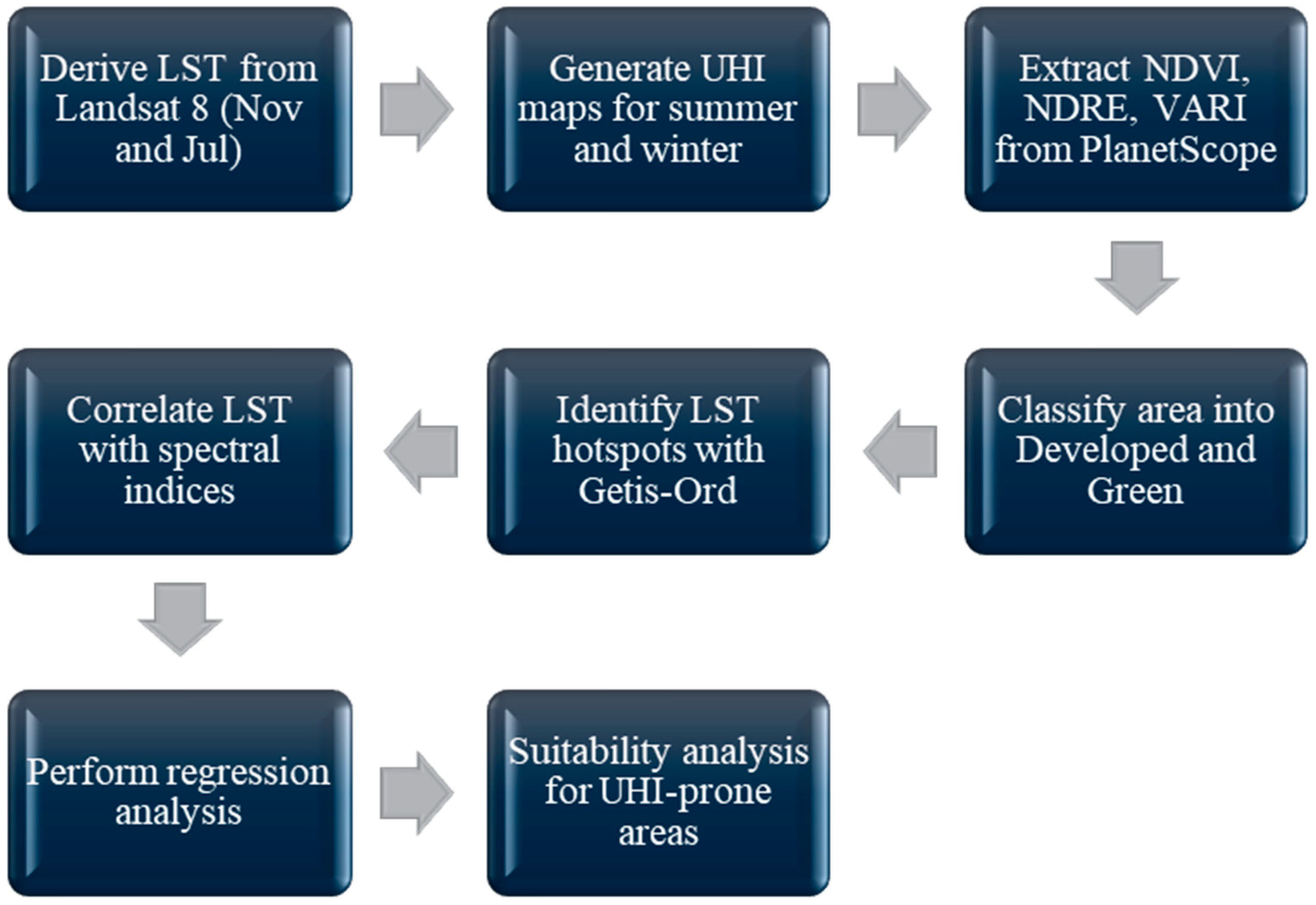
2. Methods
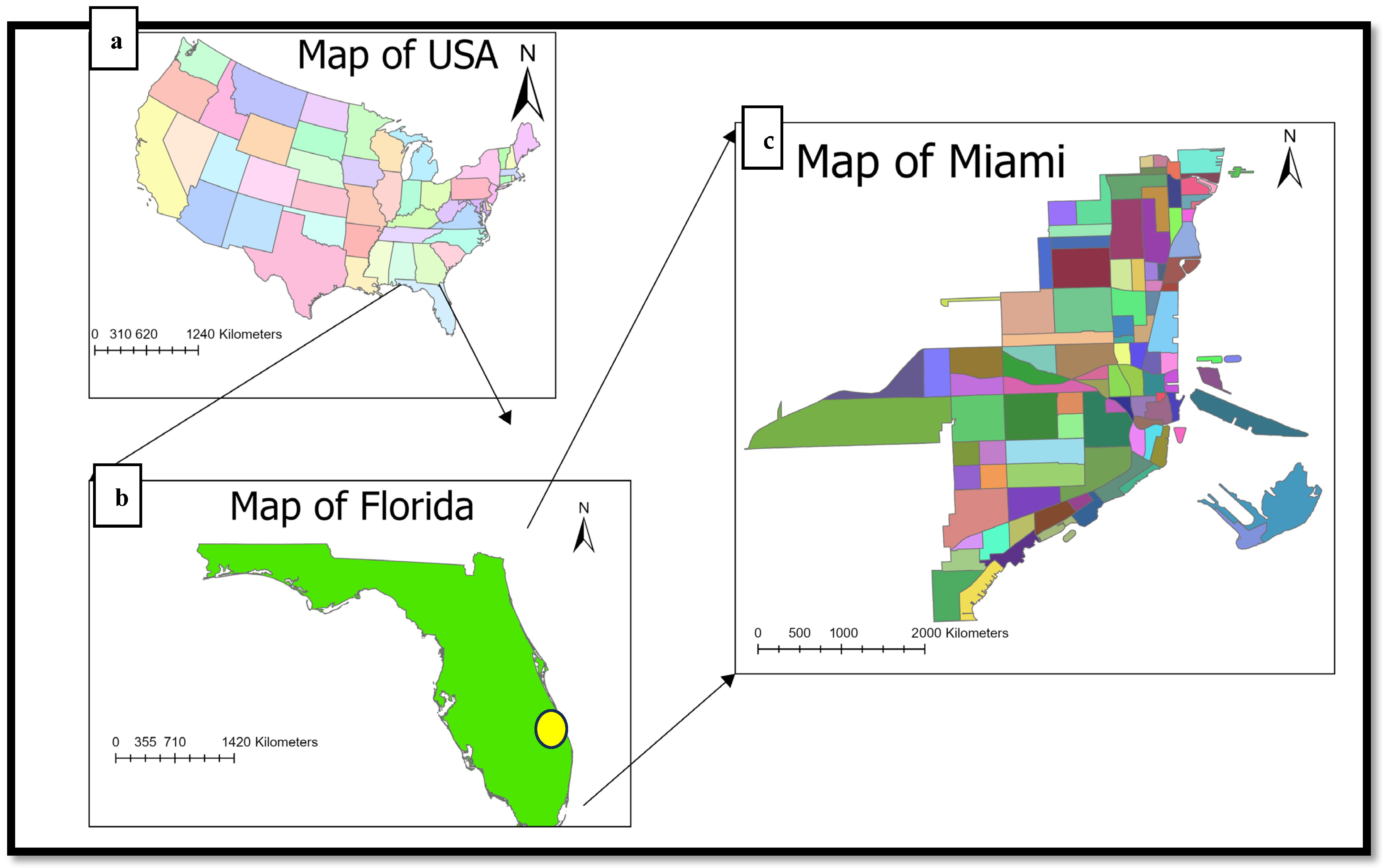
2.1. Study Area
2.2. Data Preparation
2.3. Spectral Indices and Land Cover Map from PlanetScope Data
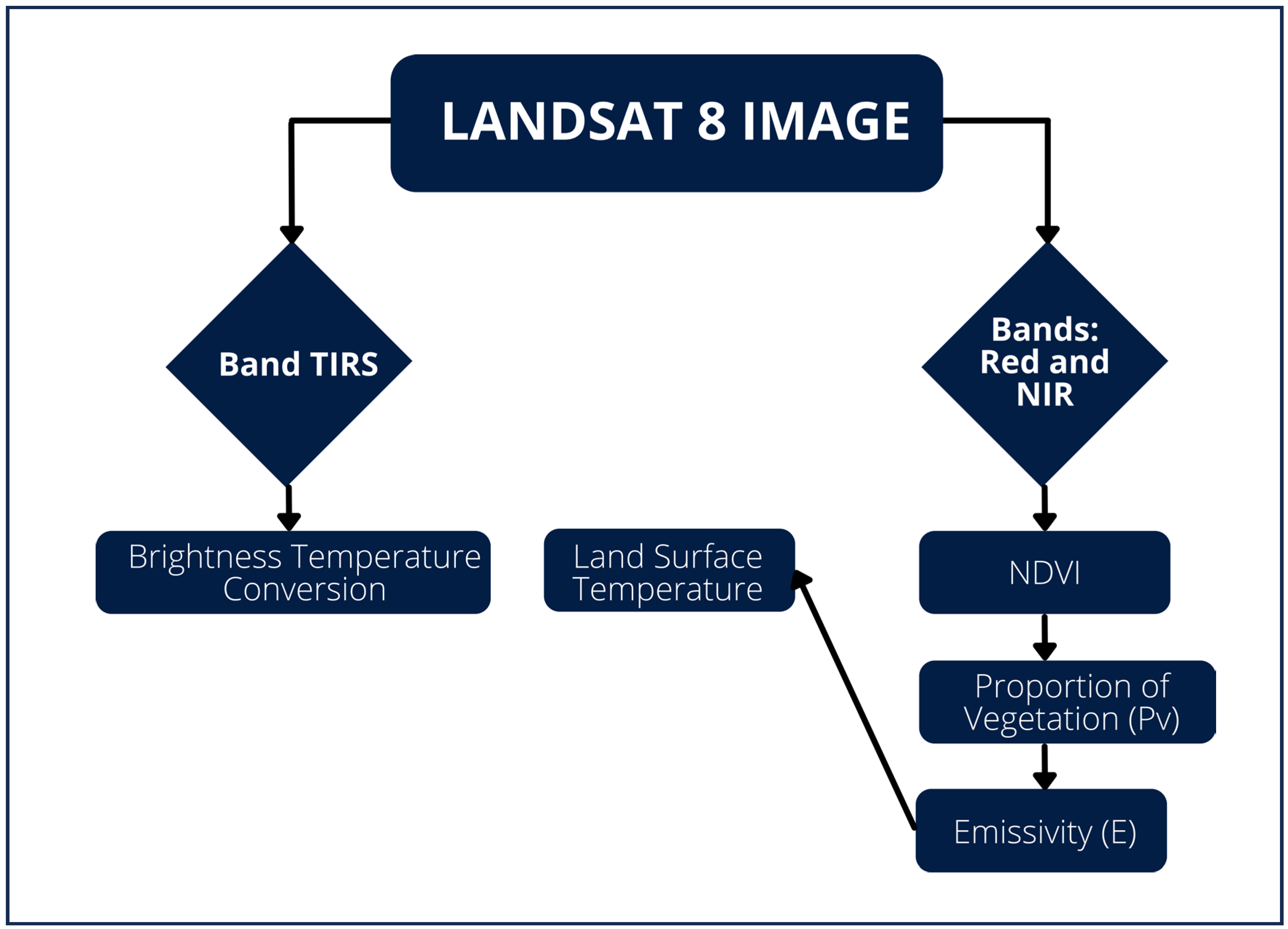
2.4. Land Surface Temperature and Urban Heat Island Raster Using Landsat 8 OLI Data
2.5. Relationship Analysis and Suitability Analysis for UHI-Prone Areas
3. Results
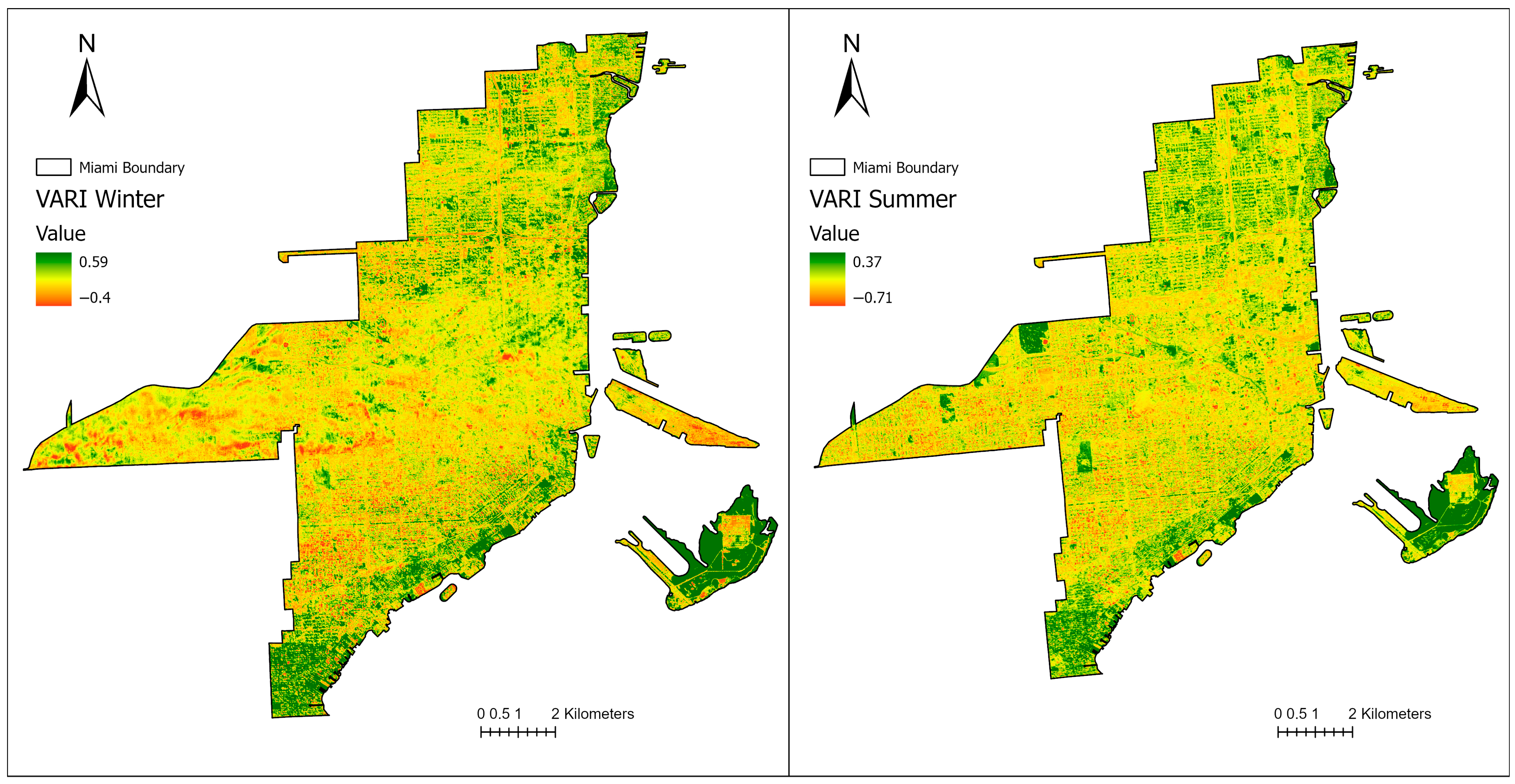
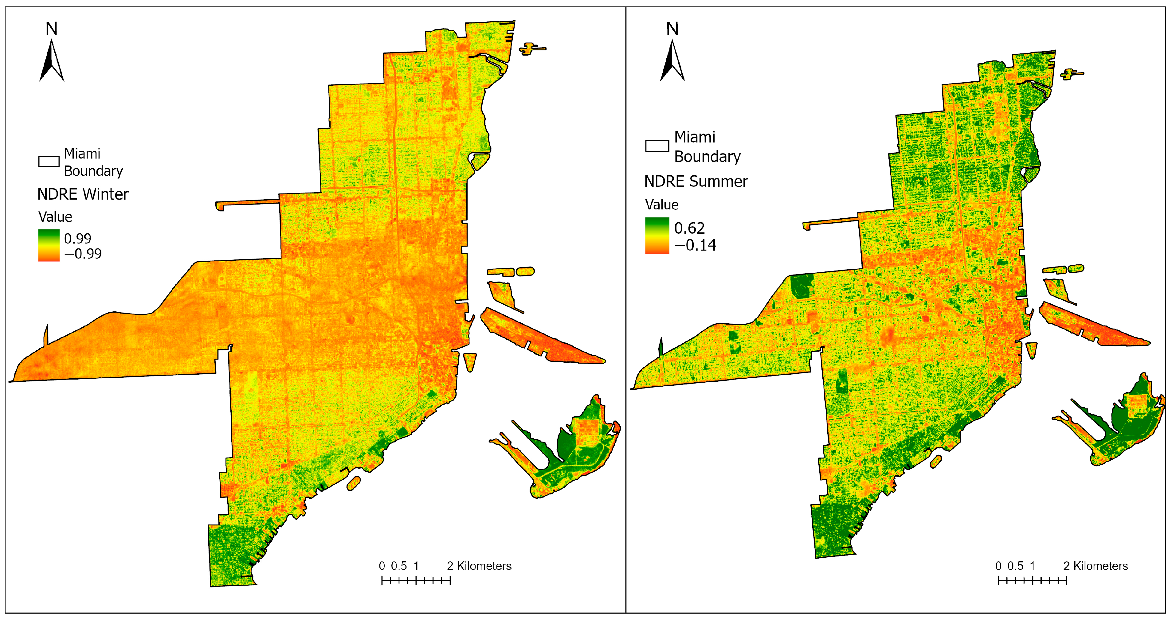
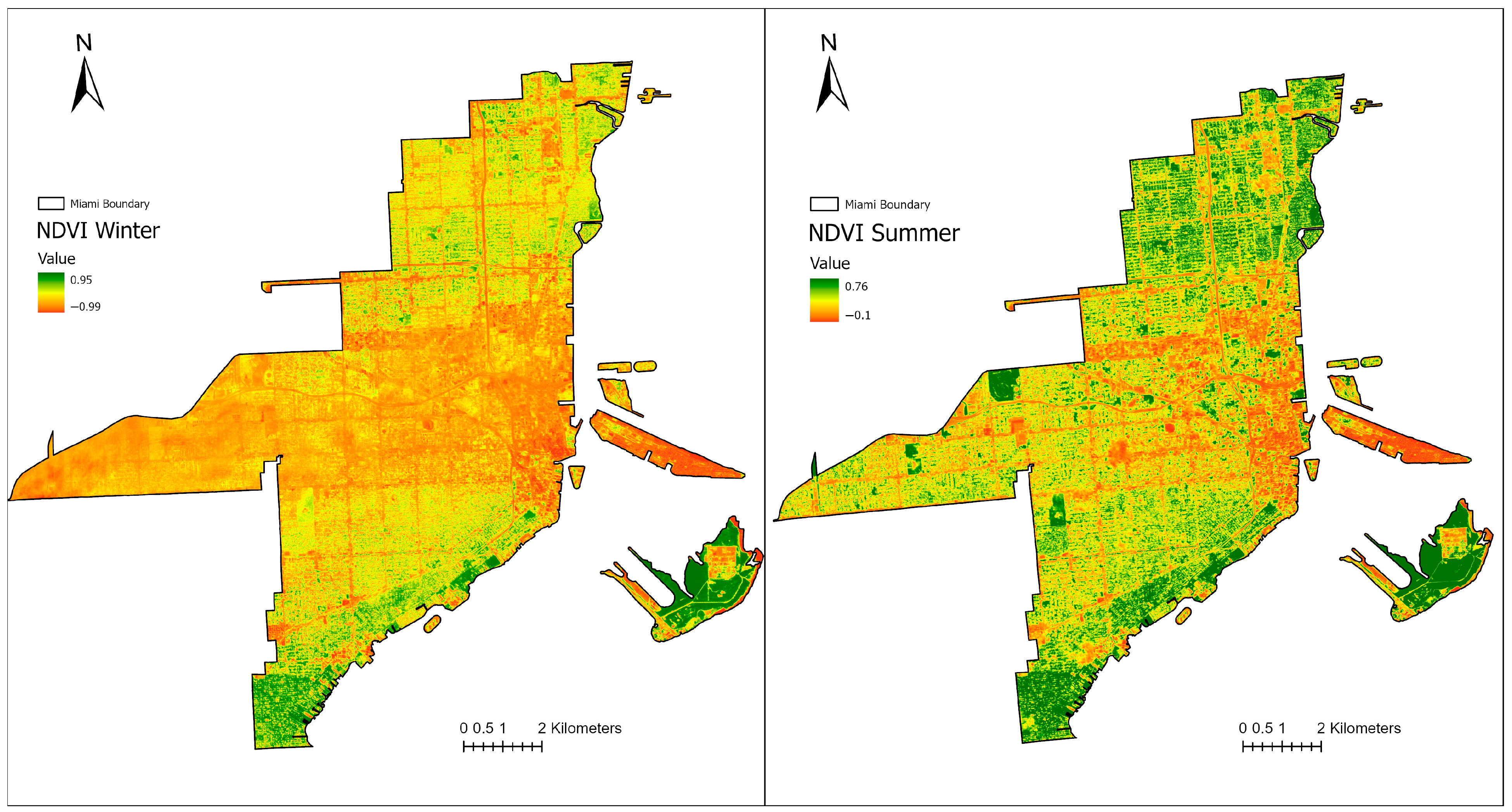
3.1. Spectral Indices of Study Area
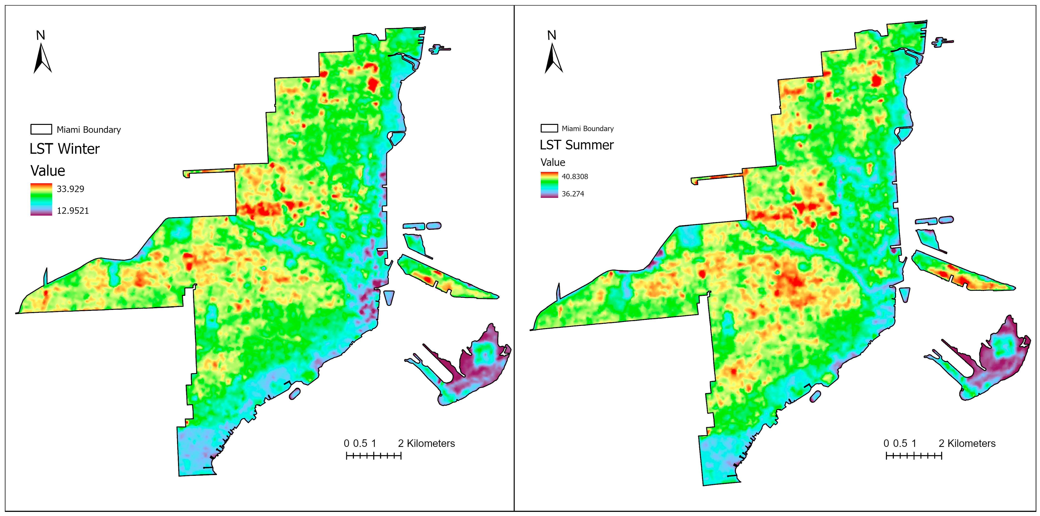
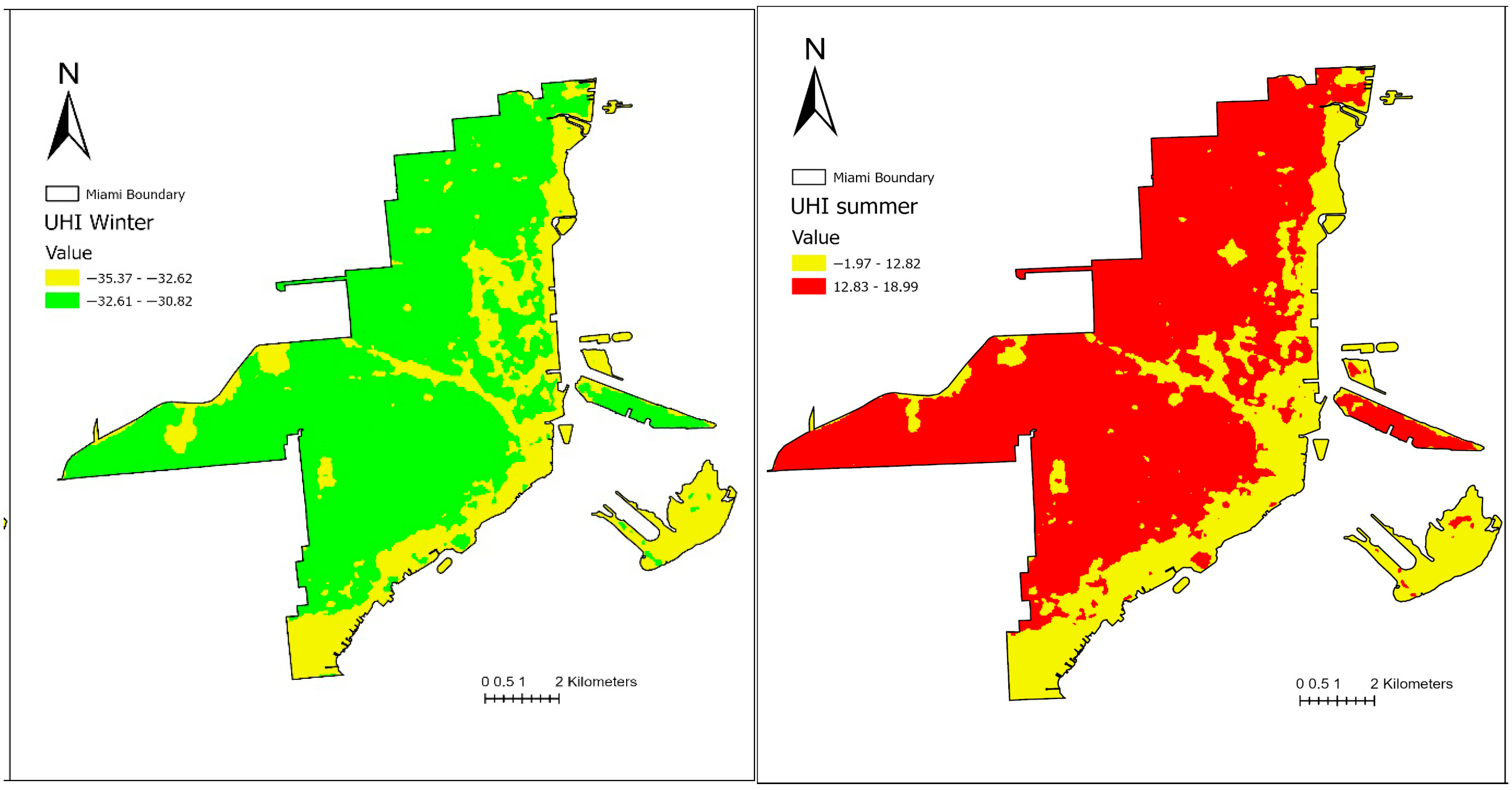
3.2. Land Surface Temperature and Urban Heat Island Raster of Study Area
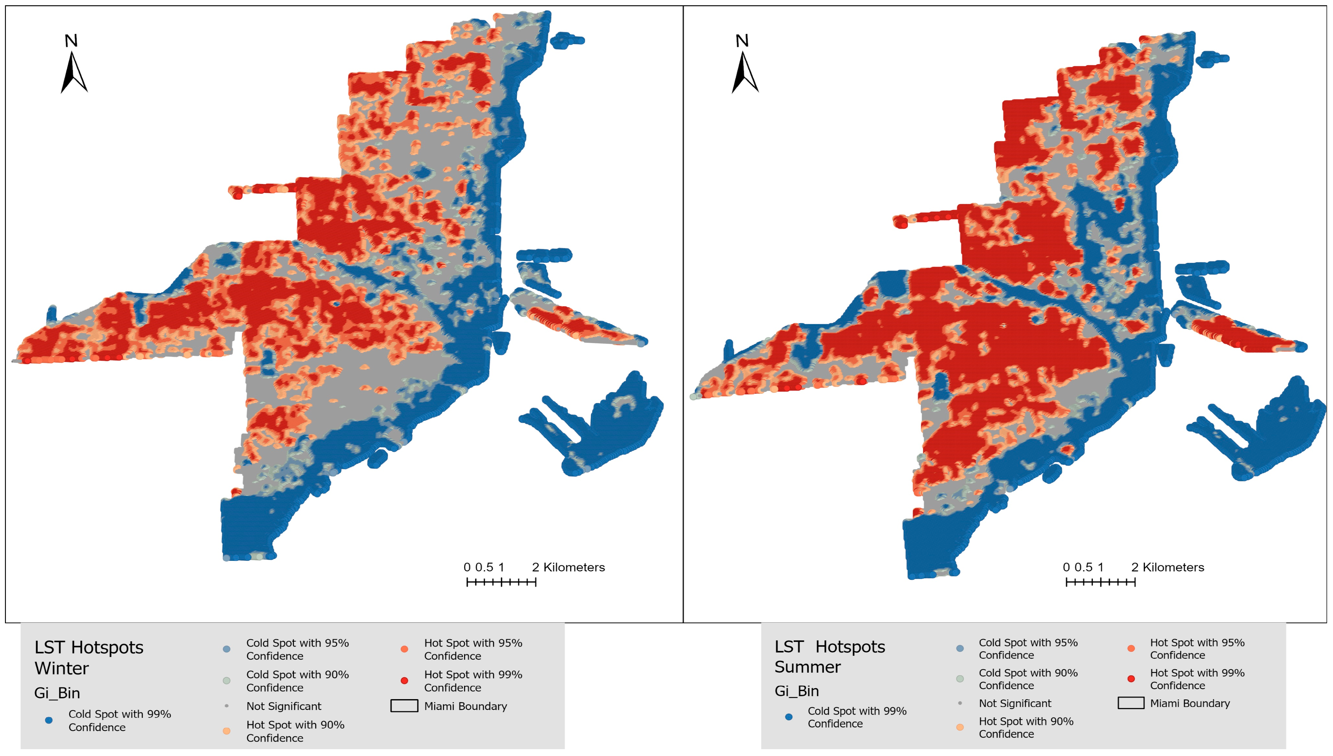
3.3. Land Surface Temperature Gi_Bin Hotspots
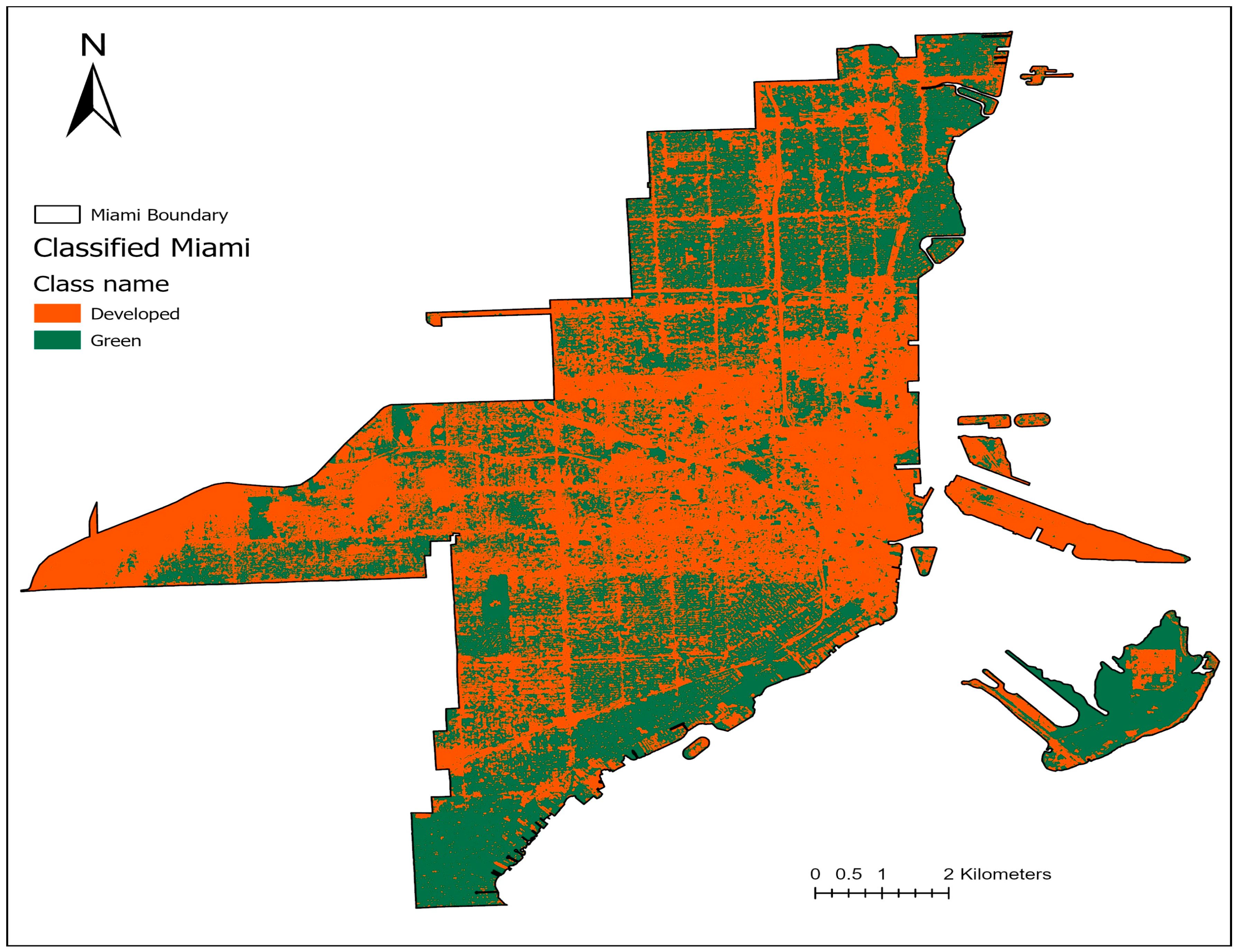
3.4. Land Cover Classification and Accuracy Assessment of Classification
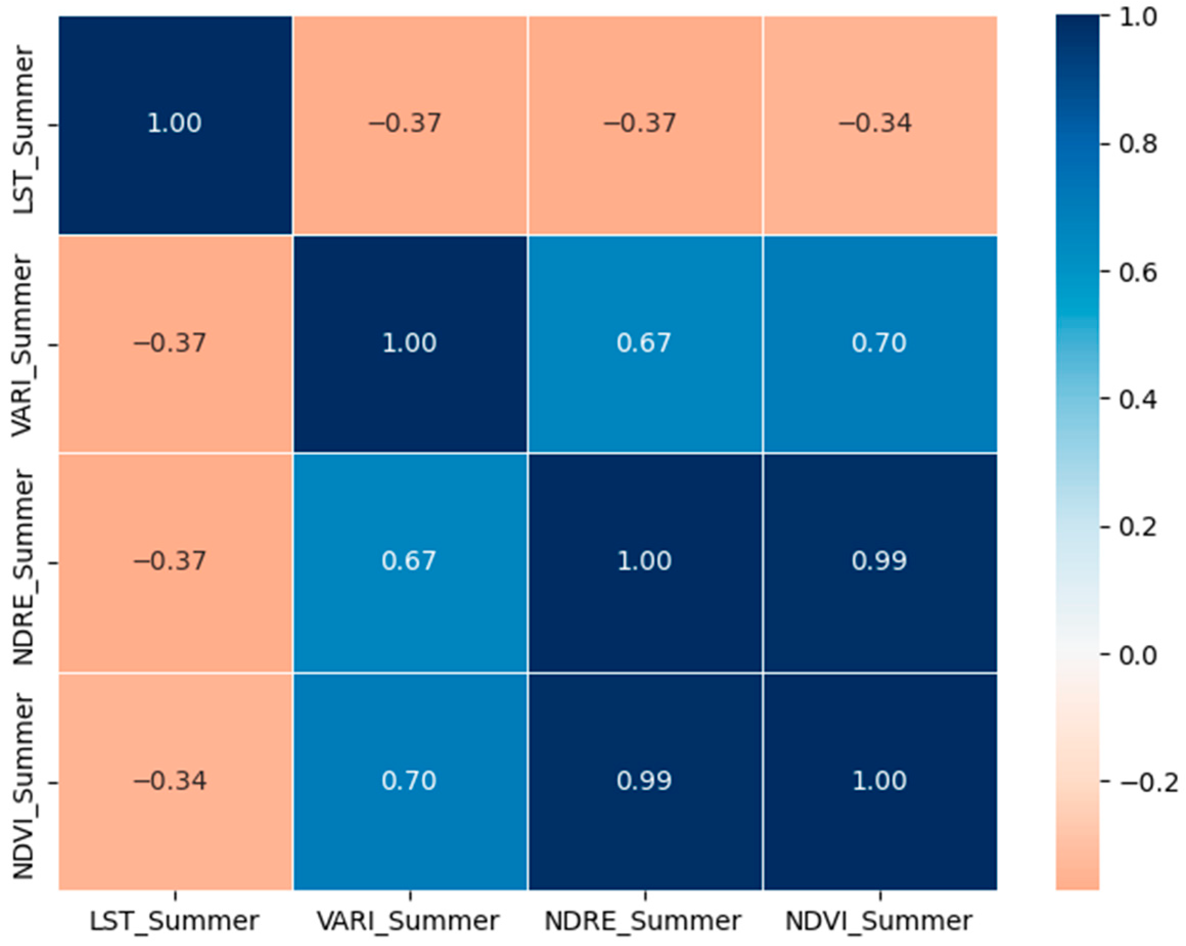
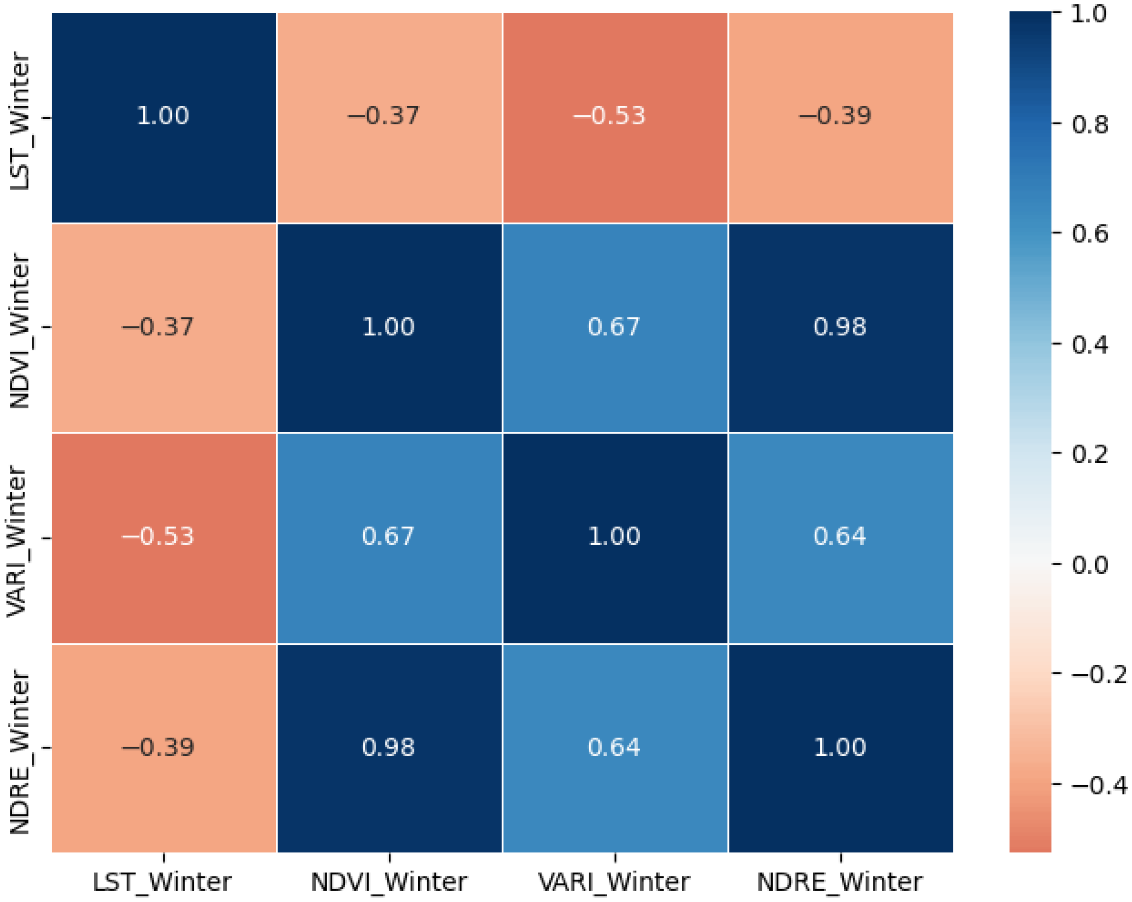
3.5. Correlation Matrices Between Vegetation Indices and Land Surface Temperature
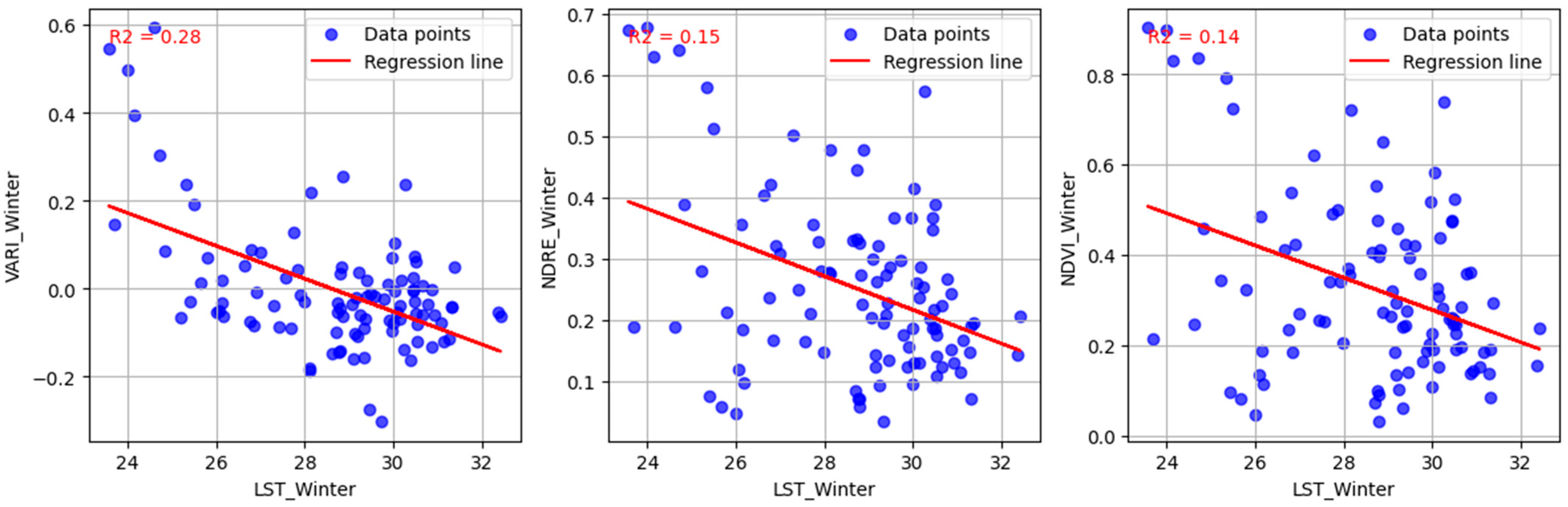
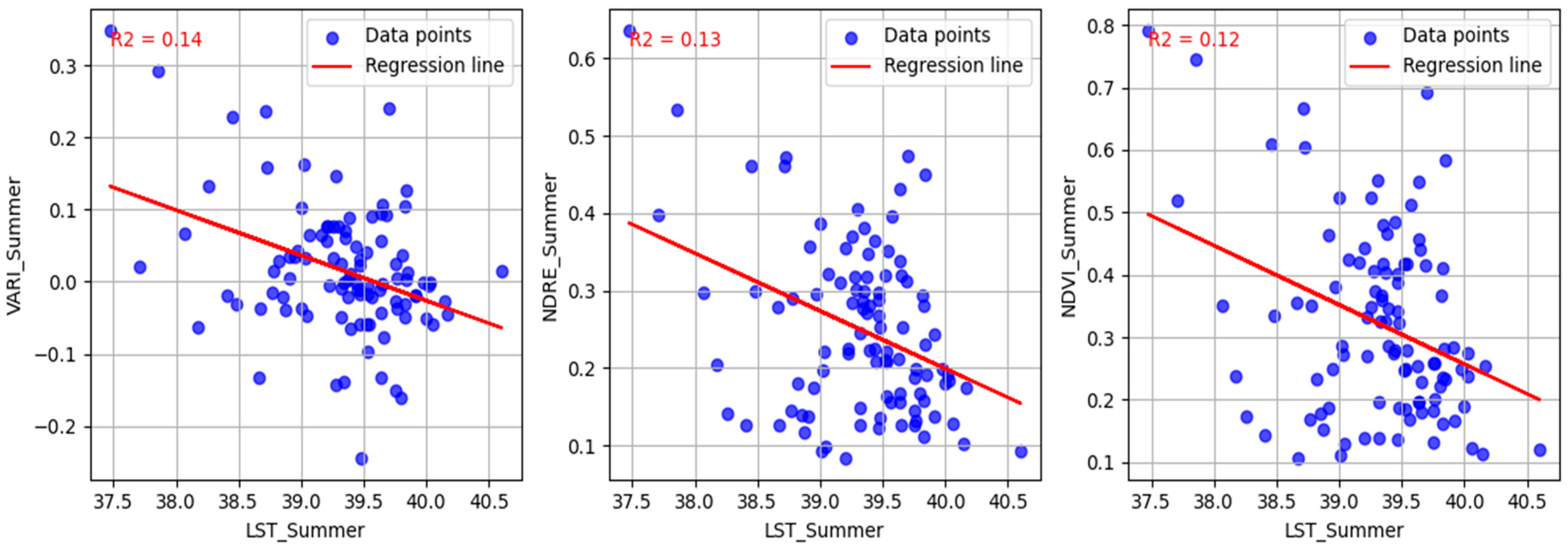
3.6. Linear Regression Between Vegetation Indices and Land Surface Temperature
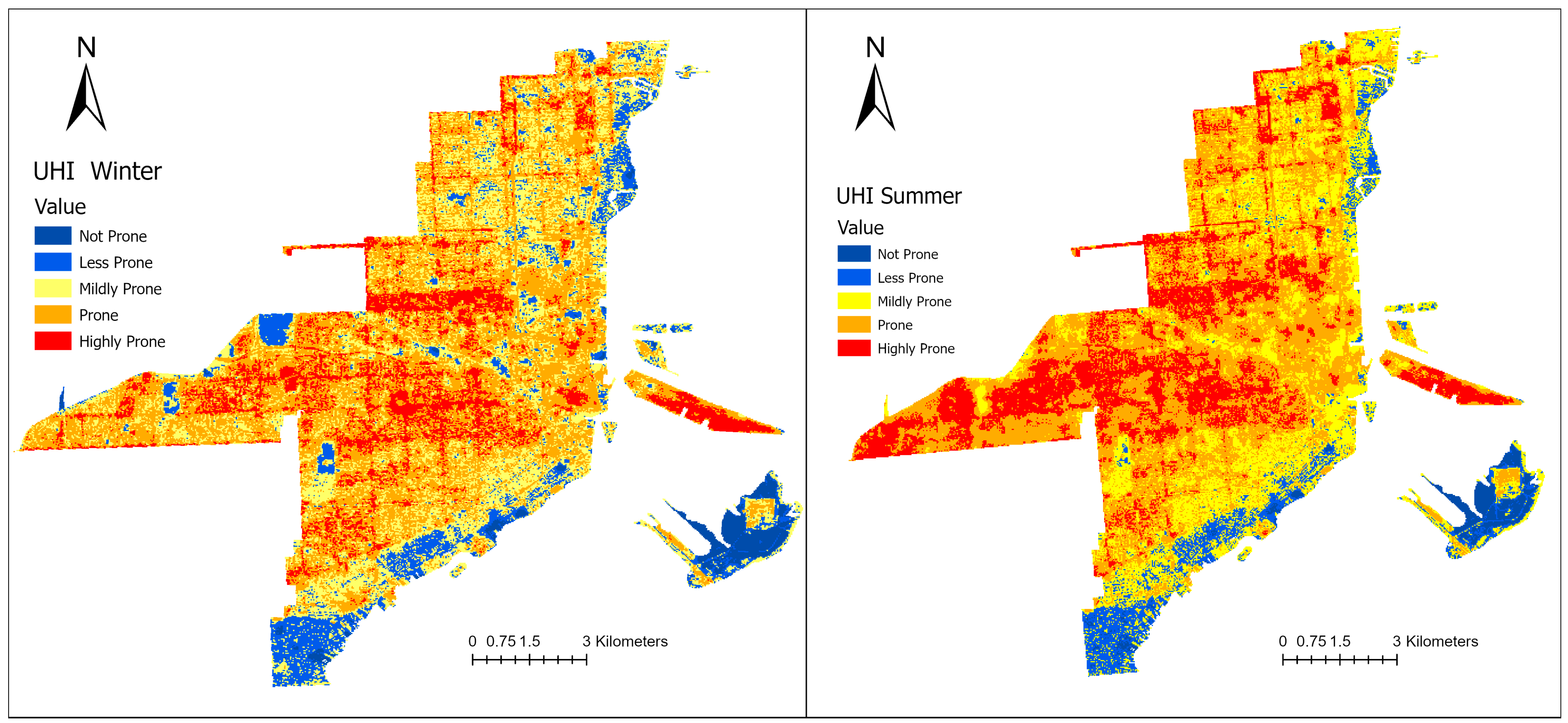
3.7. Suitability Analysis of Urban Heat Island Intensity Effect in Study Area
4. Discussion
5. Conclusions
Author Contributions
Funding
Institutional Review Board Statement
Informed Consent Statement
Data Availability Statement
Acknowledgments
Conflicts of Interest
References
- Aslan, N.; Koc-San, D. The use of land cover indices for rapid surface urban heat island detection from multi-temporal landsat imageries. ISPRS Int. J. Geo Inf. 2021, 10, 416. [Google Scholar] [CrossRef]
- United Nations. 2018 Revision of World Urbanization Prospects. 2018. Available online: https://www.un.org/en/desa/2018-revision-world-urbanization-prospects (accessed on 23 June 2023).
- Carrillo-Niquete, G.A.; Andrade, J.L.; Valdez-Lazalde, J.R.; Reyes-García, C.; Hernández-Stefanoni, J.L. Characterizing spatial and temporal deforestation and its effects on surface urban heat islands in a tropical city using Landsat time series. Landsc. Urban Plan. 2022, 217, 104280. [Google Scholar] [CrossRef]
- Kamali Maskooni, E.; Hashemi, H.; Berndtsson, R.; Daneshkar Arasteh, P.; Kazemi, M. Impact of spatiotemporal land-use and land-cover changes on surface urban heat islands in a semiarid region using Landsat data. Int. J. Digit. Earth 2021, 14, 250–270. [Google Scholar] [CrossRef]
- Amindin, A.; Pouyan, S.; Pourghasemi, H.R.; Yousefi, S.; Tiefenbacher, J.P. Spatial and temporal analysis of urban heat island using Landsat satellite images. Environ. Sci. Pollut. Res. 2021, 28, 41439–41450. [Google Scholar] [CrossRef] [PubMed]
- Xian, G.Z. Monitoring and Assessing Urban Heat Island Variations and Effects in the United States; US Geological Survey: Reston, VA, USA, 2021. [Google Scholar] [CrossRef]
- Mueller, C.; Hussain, R.; Xian, G.Z.; Shi, H.; Arab, S. Mapping the Surface Urban Heat Island effect using the Landsat Surface Temperature Product. In Proceedings of the IGARSS 2023—2023 IEEE International Geoscience and Remote Sensing Symposium, Pasadena, CA, USA, 16–21 July 2023. [Google Scholar] [CrossRef]
- Li, Z.L.; Tang, B.H.; Wu, H.; Ren, H.; Yan, G.; Wan, Z.; Trigo, I.F.; Sobrino, J.A. Satellite-derived land surface temperature: Current status and perspectives. Remote Sens. Environ. 2013, 131, 14–37. [Google Scholar] [CrossRef]
- Tran, D.X.; Pla, F.; Latorre-Carmona, P.; Myint, S.W.; Caetano, M.; Kieu, H.V. Characterizing the relationship between land use land cover change and land surface temperature. ISPRS J. Photogramm. Remote Sens. 2017, 124, 119–132. [Google Scholar] [CrossRef]
- Chakraborty, T.; Hsu, A.; Manya, D.; Sheriff, G. A spatially explicit surface urban heat island database for the United States: Characterization, uncertainties, and possible applications. ISPRS J. Photogramm. Remote Sens. 2020, 168, 74–88. [Google Scholar] [CrossRef]
- Kim, S.W.; Brown, R.D. Urban heat island (UHI) intensity and magnitude estimations: A systematic literature review. Sci. Total Environ. 2021, 779, 146389. [Google Scholar] [CrossRef] [PubMed]
- Xuan, S.; Ning, Q.; Lei, Z. Impacts of the land use transition on ecosystem services in the Dongting Lake area. Front. Environ. Sci. 2024, 12, 1422989. [Google Scholar] [CrossRef]
- Meier, J. Global Irrigation Mapping-the Role of Spatial Resolution of Current and Future Earth Observation Missions. Ph.D. Thesis, Ludwig-Maximilians-Universität München, Munich, Germany, 2023. [Google Scholar]
- Mishra, D.R.; Ghosh, S. 14 Using Moderate-Resolution Satellite Sensors for Monitoring the Biophysical Parameters and Phenology of Tidal Marshes. Remote Sens. Wetl. Appl. Adv. 2015, 283. [Google Scholar]
- Wulder, M.A.; Roy, D.P.; Radeloff, V.C.; Loveland, T.R.; Anderson, M.C.; Johnson, D.M.; Healey, S.; Zhu, Z.; Scambos, T.A.; Pahlevan, N.; et al. Fifty Years of Landsat Science and Impacts. Remote. Sens. Environ. 2022, 280, 113195. [Google Scholar] [CrossRef]
- Jimenez-Munoz, J.C.; Sobrino, J.A.; Skoković, D.; Mattar, C.; Cristobal, J. Land surface temperature retrieval methods from Landsat-8 thermal infrared sensor data. IEEE Geosci. Remote Sens. Lett. 2014, 11, 1840–1843. [Google Scholar] [CrossRef]
- Cristóbal, J.; Jiménez-Muñoz, J.C.; Prakash, A.; Mattar, C.; Skoković, D.; Sobrino, J.A. An improved single-channel method to retrieve land surface temperature from the Landsat-8 thermal band. Remote Sens. 2018, 10, 431. [Google Scholar] [CrossRef]
- Fu, P.; Weng, Q. A time series analysis of urbanization induced land use and land cover change and its impact on land surface temperature with Landsat imagery. Remote Sens. Environ. 2016, 175, 205–214. [Google Scholar] [CrossRef]
- Dewan, A.M.; Yamaguchi, Y. Land use and land cover change in Greater Dhaka, Bangladesh: Using remote sensing to promote sustainable urbanization. Appl. Geogr. 2009, 29, 390–401. [Google Scholar] [CrossRef]
- Frazier, A.E.; Hemingway, B.L. A technical review of planet smallsat data: Practical considerations for processing and using planetscope imagery. Remote Sens. 2021, 13, 3930. [Google Scholar] [CrossRef]
- Csillik, O.; Kumar, P.; Mascaro, J.; O’Shea, T.; Asner, G.P. Monitoring tropical forest carbon stocks and emissions using Planet satellite data. Sci. Rep. 2019, 9, 17831. [Google Scholar] [CrossRef] [PubMed]
- Wu, H.; Gui, Z.; Yang, Z. Geospatial big data for urban planning and urban management. Geo Spat. Inf. Sci. 2020, 23, 273–274. [Google Scholar] [CrossRef]
- Sozzi, M.; Marinello, F.; Pezzuolo, A.; Sartori, L. Benchmark of satellites image services for precision agricultural use. In Proceedings of the AgEng Conference, Wageningen, The Netherlands, 8–12 July 2018; pp. 8–11. [Google Scholar]
- Li, J.; Knapp, D.E.; Schill, S.R.; Roelfsema, C.; Phinn, S.; Silman, M.; Mascaro, J.; Asner, G.P. Adaptive bathymetry estimation for shallow coastal waters using Planet Dove satellites. Remote Sens. Environ. 2019, 232, 111302. [Google Scholar] [CrossRef]
- Pascual, A.; Tupinambá-Simões, F.; Guerra-Hernández, J.; Bravo, F. High-resolution planet satellite imagery and multi-temporal surveys to predict risk of tree mortality in tropical eucalypt forestry. J. Environ. Manag. 2022, 310, 114804. [Google Scholar] [CrossRef] [PubMed]
- Roy, D.P.; Huang, H.; Houborg, R.; Martins, V.S. A global analysis of the temporal availability of PlanetScope high spatial resolution multi-spectral imagery. Remote Sens. Environ. 2021, 264, 112586. [Google Scholar] [CrossRef]
- Battles, A.C.; Kolbe, J.J. Miami heat: Urban heat islands influence the thermal suitability of habitats for ectotherms. Glob. Change Biol. 2019, 25, 562–576. [Google Scholar] [CrossRef] [PubMed]
- Sun, Y.; Augenbroe, G. Urban heat island effect on energy application studies of office buildings. Energy Build. 2014, 77, 171–179. [Google Scholar] [CrossRef]
- Ju, J.; Roy, D.P. The availability of cloud-free Landsat ETM+ data over the conterminous United States and globally. Remote Sens. Environ. 2008, 112, 1196–1211. [Google Scholar] [CrossRef]
- Xiao, C.; Li, P.; Feng, Z.; Wu, X. Spatio-temporal differences in cloud cover of Landsat-8 OLI observations across China during 2013–2016. J. Geogr. Sci. 2018, 28, 429–444. [Google Scholar] [CrossRef]
- Xu, S.; Yu, T.; Xu, J.; Pan, X.; Shao, W.; Zuo, J.; Yu, Y. Monitoring and Forecasting Green Tide in the Yellow Sea Using Satellite Imagery. Remote Sens. 2023, 15, 2196. [Google Scholar] [CrossRef]
- Rouse, J.W.; Hass, R.H.; Schell, J.A.; Deering, D.W.; Harlan, J.C. Monitoring the Vernal Advancement and Retrogradation (Green Wave Effect) of Natural Vegetation; Final Report, RSC 1978-4; Texas A & M University: College Station, TX, USA, 1974; pp. 1–120. [Google Scholar]
- Gitelson, A.A.; Merzlyak, M.N. Remote estimation of chlorophyll content in higher plant leaves. Int. J. Remote Sens. 1997, 18, 2691–2697. [Google Scholar] [CrossRef]
- Grover, A.; Singh, R.B. Analysis of Urban Heat Island (UHI) in Relation to Normalized Difference Vegetation Index (NDVI): A Comparative Study of Delhi and Mumbai. Environments 2015, 2, 125–138. [Google Scholar] [CrossRef]
- Mostofi, N.; Hasanlou, M. Feature selection of various land cover indices for monitoring surface heat island in Tehran city using Landsat 8 imagery. J. Environ. Eng. Landsc. Manag. 2017, 25, 241–250. [Google Scholar] [CrossRef]
- Matlan, S.J.; Abdullah, S.; Alias, R.; Mukhlisin, M. Effect of working rainfall and soil water index on slope stability in Ranau, Sabah. Int. J. Civ. Eng. Technol. 2018, 9, 1331–1341. [Google Scholar]
- Suribabu, C.R.; Sujatha, E.R. Evaluation of moisture level using precipitation indices as a landslide triggering factor-a study of Coonoor Hill Station. Climate 2019, 7, 111. [Google Scholar] [CrossRef]
- Monsieurs, E.; Dewitte, O.; Demoulin, A. A susceptibility-based rainfall threshold approach for landslide occurrence. Nat. Hazards Earth Syst. Sci. 2019, 19, 775–789. [Google Scholar] [CrossRef]
- Segoni, S.; Rosi, A.; Lagomarsino, D.; Fanti, R.; Casagli, N. Brief communication: Using averaged soil moisture estimates to improve the performances of a regional-scale landslide early warning system. Nat. Hazards Earth Syst. Sci. 2018, 18, 807–812. [Google Scholar] [CrossRef]
- Zhao, Q.; Qu, Y. The Retrieval of Ground NDVI (Normalized Difference Vegetation Index) Data Consistent with Remote-Sensing Observations. Remote Sens. 2024, 16, 1212. [Google Scholar] [CrossRef]
- Eastman, J.R.; Sangermano, F.; Machado, E.A.; Rogan, J.; Anyamba, A. Global Trends in Seasonality of Normalized Difference Vegetation Index (NDVI), 1982–2011. Remote Sens. 2013, 5, 4799–4818. [Google Scholar] [CrossRef]
- Fayech, D.; Tarhouni, J. Climate variability and its effect on normalized difference vegetation index (NDVI) using remote sensing in semi-arid area. Model. Earth Syst. Environ. 2021, 7, 1667–1682. [Google Scholar] [CrossRef]
- Mazzarino, M.; Finn, J.T. An NDVI analysis of vegetation trends in an Andean watershed. Wetl. Ecol. Manag. 2016, 24, 623–640. [Google Scholar] [CrossRef]
- Shapiro, A.D.; Liu, W. Evaluating Land Surface Temperature Trends and Explanatory Variables in the Miami Metropolitan Area from 2002–2021. Geomatics 2024, 4, 1–16. [Google Scholar] [CrossRef]
- Xian, G.Z. Characterizing Urban Heat Islands Across 50 Major Cities in the United States; US Geological Survey: Reston, VA, USA, 2023. [Google Scholar] [CrossRef]
- Shi, H.; Xian, G.; Auch, R.; Gallo, K.; Zhou, Q. Urban Heat Island and Its Regional Impacts Using Remotely Sensed Thermal Data—A Review of Recent Developments and Methodology. Land 2021, 10, 867. [Google Scholar] [CrossRef]
- Rendana, M.; Idris, W.M.R.; Rahim, S.A.; Abdo, H.G.; Almohamad, H.; Al Dughairi, A.A.; Al-Mutiry, M. Relationships between land use types and urban heat island intensity in Hulu Langat district, Selangor, Malaysia. Ecol. Process. 2023, 12, 33. [Google Scholar] [CrossRef]
- Guha, S.; Govil, H. Land surface temperature and normalized difference vegetation index relationship: A seasonal study on a tropical city. SN Appl. Sci. 2020, 2, 1661. [Google Scholar] [CrossRef]
- Garai, S.; Khatun, M.; Singh, R.; Sharmaet, J.; Pradhan, M.; Ranjan, A.; Rahaman, S.M.; Khan, M.L.; Tiwari, S. Assessing correlation between Rainfall, normalized difference Vegetation Index (NDVI) and land surface temperature (LST) in Eastern India. Saf. Extrem. Environ. 2022, 4, 119–127. [Google Scholar] [CrossRef]
- Sharma, M.; Bangotra, P.; Gautam, A.S.; Gautam, S. Sensitivity of normalized difference vegetation index (NDVI) to land surface temperature, soil moisture and precipitation over district Gautam Buddh Nagar, UP, India. Stoch. Environ. Res. Risk Assess. 2022, 36, 1779–1789. [Google Scholar] [CrossRef] [PubMed]
- Kikon, N.; Kumar, D.; Ahmed, S.A. Quantitative assessment of land surface temperature and vegetation indices on a kilometer grid scale. Environ. Sci. Pollut. Res. 2023, 30, 107236–107258. [Google Scholar] [CrossRef] [PubMed]
- Hussain, S.; Raza, A.; Abdo, H.G.; Mubeen, M.; Tariq, A.; Nasim, W.; Majeed, M.; Almohamad, H.; Dughairi, A.A.A. Relation of land surface temperature with different vegetation indices using multi-temporal remote sensing data in Sahiwal region, Pakistan. Geosci. Lett. 2023, 10, 33. [Google Scholar] [CrossRef]
- Sharma, K.V.; Khandelwal, S.; Kaul, N. Downscaling of Coarse Resolution Land Surface Temperature Through Vegetation Indices Based Regression Models BT–Applications of Geomatics in Civil Engineering; Ghosh, J.K., da Silva, I., Eds.; Springer: Berlin/Heidelberg, Germany, 2020; pp. 625–636. [Google Scholar]
- Jaber, S.M. Insights About the Spatial and Temporal Characteristics of the Relationships Between Land Surface Temperature and Vegetation Abundance and Topographic Elements in Arid to Semiarid Environments. Remote Sens. Earth Syst. Sci. 2023, 6, 254–274. [Google Scholar] [CrossRef]
- Cui, Y.Y.; de Foy, B. Seasonal Variations of the Urban Heat Island at the Surface and the Near-Surface and Reductions due to Urban Vegetation in Mexico City. J. Appl. Meteorol. Climatol. 2012, 51, 855–868. [Google Scholar] [CrossRef]
- Almeida, C.R.; Teodoro, A.C.; Gonçalves, A. Study of the Urban Heat Island (UHI) Using Remote Sensing Data/Techniques: A Systematic Review. Environments 2021, 8, 105. [Google Scholar] [CrossRef]
- Li, J.; Sun, R.; Liu, T.; Xie, W.; Chen, L. Prediction models of urban heat island based on landscape patterns and anthropogenic heat dynamics. Landsc. Ecol. 2021, 36, 1801–1815. [Google Scholar] [CrossRef]
- Zhou, B.; Rybski, D.; Kropp, J.P. On the statistics of urban heat island intensity. Geophys. Res. Lett. 2013, 40, 5486–5491. [Google Scholar] [CrossRef]
- Wu, X.; Zhang, L.; Zang, S. Examining seasonal effect of urban heat island in a coastal city. PLoS ONE 2019, 14, e0217850. [Google Scholar] [CrossRef] [PubMed]
- Kedzuf, N.J.; Zuidema, P.; Mcnoldy, B. Seasonal Variability and Trends of the Miami Urban Island. Amer. Met. Soc. 2011, 98, 1–6. Available online: https://bmcnoldy.earth.miami.edu/papers/KZM2018_98AMS_ext.pdf (accessed on 11 May 2025).
- Hari Kandel, A.M.; Whitman, D. An analysis on the urban heat island effect using radiosonde profiles and Landsat imagery with ground meteorological data in South Florida. Int. J. Remote Sens. 2016, 37, 2313–2337. [Google Scholar] [CrossRef]

| Data | Spatial Resolution | Source of Data | Types of Data | Acquisition Months |
|---|---|---|---|---|
| Landsat data 2023 | 30 m | USGS/EROS | Raster | July and November |
| PlanetScope Scene Data 2023 | 3–7 m | PlanetScope | COG (Cloud Optimized Geo Tiff) Raster | July and November |
| PlanetScope data acquired for this study | ||||
| July 2023 Data | November 2023 Data | |||
| 20230723_150912_76_2458 | 20231106_154948_35_2498 | |||
| 20230723_150909_77_24af | 20231106_154946_30_2498 | |||
| 20230723_150907_48_24af | 20231106_154944_24_2498 | |||
| 20230723_150905_18_24af | 20231106_154942_19_2498 | |||
| 20230723_150654_80_24ca | 20231106_154900_24_249a | |||
| 20230723_150652_51_24ca | 20231106_154858_19_249a | |||
| 20230723_150650_21_24ca | 20231106_154856_15_249a | |||
| Landsat data acquired for this study | ||||
| Data Set Identifier | Cloud Cover % | WRS Path | WRS Row | |
| LC08_L2SP_015042_20231111_20231117_02_T1 | 12.78 | 015 | 042 | |
| LC08_L2SP_015042_20230706_20230717_02_T1 | 16.39 | 015 | 042 | |
| Vegetation Indices | Formula |
|---|---|
| NDVI (Normalized Difference Vegetation Index) | (NIR − R)/(NIR + R) [32] |
| NDRE (Normalized Difference Red Edge Index) | (NIR − RE)/(NIR + RE) [33] |
| VARI (Visible Atmospherically Resistant Index) | (G − R)/(G + R − B) [33] |
| OBJECTID | Value | Count | Area (Sq km) | Class Name |
|---|---|---|---|---|
| 1 | 0 | 7983947 | 71.86 | Developed |
| 2 | 1 | 2963656 | 26.67 | Green |
| Total Area | 98.53 | |||
| OBJECTID | Class Value | C_0 | C_1 | Total | U_Accuracy | Kappa | Class Name |
|---|---|---|---|---|---|---|---|
| 1.00 | C_0 | 48.00 | 3.00 | 51.00 | 0.94 | 0.00 | Developed |
| 2.00 | C_1 | 6.00 | 43.00 | 49.00 | 0.88 | 0.00 | Green |
| 3.00 | Total | 54.00 | 46.00 | 100.00 | 0.00 | 0.00 | |
| 4.00 | P_Accuracy | 0.89 | 0.93 | 0.00 | 0.91 | 0.00 | |
| 5.00 | Kappa | 0.00 | 0.00 | 0.00 | 0.00 | 0.82 |
Disclaimer/Publisher’s Note: The statements, opinions and data contained in all publications are solely those of the individual author(s) and contributor(s) and not of MDPI and/or the editor(s). MDPI and/or the editor(s) disclaim responsibility for any injury to people or property resulting from any ideas, methods, instructions or products referred to in the content. |
© 2025 by the authors. Licensee MDPI, Basel, Switzerland. This article is an open access article distributed under the terms and conditions of the Creative Commons Attribution (CC BY) license (https://creativecommons.org/licenses/by/4.0/).
Share and Cite
K C, S.; Chiluwal, A.; Magar, L.P.; Paudel, K. Investigating Urban Heat Islands in Miami, Florida, Utilizing Planet and Landsat Satellite Data. Atmosphere 2025, 16, 880. https://doi.org/10.3390/atmos16070880
K C S, Chiluwal A, Magar LP, Paudel K. Investigating Urban Heat Islands in Miami, Florida, Utilizing Planet and Landsat Satellite Data. Atmosphere. 2025; 16(7):880. https://doi.org/10.3390/atmos16070880
Chicago/Turabian StyleK C, Suraj, Anuj Chiluwal, Lalit Pun Magar, and Kabita Paudel. 2025. "Investigating Urban Heat Islands in Miami, Florida, Utilizing Planet and Landsat Satellite Data" Atmosphere 16, no. 7: 880. https://doi.org/10.3390/atmos16070880
APA StyleK C, S., Chiluwal, A., Magar, L. P., & Paudel, K. (2025). Investigating Urban Heat Islands in Miami, Florida, Utilizing Planet and Landsat Satellite Data. Atmosphere, 16(7), 880. https://doi.org/10.3390/atmos16070880