Temperature Prediction at Street Scale During a Heat Wave Using Random Forest

Abstract

The rising frequency of heatwaves, combined with the urban heat island effect, increases the population’s exposure to high temperatures, significantly impacting the health of vulnerable groups and the overall well-being of residents. While mesoscale meteorological models can reliably forecast temperatures across urban neighbourhoods, dense networks of in situ measurements offer more precise data at the street scale. In this work, the Random Forest technique was used to predict street-scale temperatures in the downtown area of Thessaloniki, Greece, during a prolonged heatwave in July 2021. The model was trained using data from a low-cost sensor network, meteorological fields calculated by the mesoscale model MEMO, and micro-environmental spatial features. The results show that, although the MEMO temperature predictions achieve high accuracy during nighttime compared to measurements, they exhibit inconsistent trends across sensor locations during daytime, indicating that the model does not fully account for microclimatic phenomena. Additionally, by using only the observed temperature as the target of the Random Forest model, higher accuracy is achieved, but spatial features are not represented in the predictions. In contrast, the most reliable approach to incorporating spatial characteristics is to use the difference between observed and mesoscale temperatures as the target variable.

1. Introduction

Numerical Weather Prediction (NWP) models have been used to provide urbanized temperature fields, taking into account the effect of urban canopy, coverage type and anthropogenic forcing [1,2]. The development of urbanized surface parametrizations over the last couple of decades has vastly improved NWP skills in simulating urban radiative and thermal effects, including the urban heat island (UHI), particularly at the mesoscale and local scales [3,4]. Contributions of surface budget modification, urban coverage types, radiation trapping and shading have been introduced in various urban modelling schemes, either as explicit processes-based modules [5] or by appropriate modifications to the surface thermal budget and radiative transfer mechanisms already present in NWP models [6]. Most of these improvements aim to enhance the model’s potential to provide short- and medium-term predictions on temperature and radiation at the local scale (of the order of a few hundred meters), effectively downscaling the driving regional or mesoscale meteorology to specific land coverages associated with the urban canopy. Despite the obvious improvements in predicting local forcings and the improved overall skill of NWP models in reproducing thermal and weather patterns at the respective scales, they offer limited insights on thermal effects, which define thermal exposure in urban microenvironments, compared to explicit 3D microscale models [7]. On the other hand, accurate modelling of such exposures can benefit from using the coarser-resolution NPW fields as boundary conditions, where additional effects of land cover, structure of surrounding buildings, ventilation, surface properties, and orientation, as well as shading geometry are accounted for by explicit microscale modelling or by a surrogate model [8].

Machine learning utilization has increased in the field of weather and climate modelling, especially over the past 10 years, during which these types of models have become competitive with the corresponding process-based models [9]. In addition to directly predicting weather and environmental variables, a wide range of machine learning applications are now being integrated with numerical models, including NWP downscaling [10]. As shown in the review paper by de Burgh-Day and Leeuwenburg [9], the vast majority of NWP and machine learning integrations rely on neural networks for prediction. However, a significant number of earlier studies have used decision tree-based methods, particularly Random Forest algorithms [11,12,13,14,15].

Meenal et al. [11] compared the performance of Random Forest and Super Vector Machine (SVM) models for predicting solar radiation and wind speed in Tamil Nadu, India, and found that Random Forest achieved significantly higher accuracy than SVM for both parameters. In a study by Goutham et al. [12], it was shown that the use of Random Forest can reduce errors in NWP-derived surface wind speed forecasts from the European Centre for Medium-Range Weather Forecasts (ECMWF) in regions of France and Corsica. Shin et al. [13] evaluated several machine learning methods combined with an NWP model to downscale wind speed predictions for agricultural applications at a high spatial resolution of 100 × 100 m in South Korea and found that Random Forest produced the best results.

In addition to forecasting regulated environmental parameters, a crucial area of research in NWP modelling is the investigation of extreme weather events. Such events pose significant risks to both public health [16] and the environment and also impact various economic sectors, including agriculture. Extreme weather events have increased dramatically in recent years and are expected to become even more frequent due to the climate crisis [17]. Das et al. [14] employed a Random Forest model for intense rainfall nowcasting. Similarly, in the study by Yao et al. [15], a Random Forest algorithm was used to predict hailstorms in the Shandong Peninsula, China.

Recently, significant progress has been made in the use of machine learning algorithms for downscaling NWP models at various scales for temperature prediction purposes, often in combination with in situ or remote sensing measurements. In such studies, either the observed temperature ($T_{obs}$) or the difference between the observed and NWP-predicted temperature ($\mathsf{\Delta }T$) has been used as the target variable. In the work of Chajaei and Bagheri [18], data from the urban climate model UrbClim were combined with morphological features extracted from LiDAR data to train several machine learning algorithms for predicting $T_{obs}$ at street scale. They found that the LightGBM model provided the best performance. Bhakare et al. [19] compared Random Forest (RF), Artificial Neural Networks (ANNs), and Convolutional Neural Networks (CNNs) for downscaling ERA5-Land reanalysis temperature data from 9 km to 1 km over a domain that included the Non Valley and the Adige Valley in the Italian Alps. They found that Random Forest outperformed ANN and yielded comparable results to CNN, particularly during the summer and spring, but accuracy declined during winter and autumn.

Blun et al. [20] downscaled regional UKV model heatwave temperature predictions from 1 km to 100 m horizontal resolution using $\mathsf{\Delta }T$ as the target variable, applying Random Forest, XGBoost, and Multilayer Perceptron algorithms. They found that all three machine learning methods provided similar accuracy. Shin and Yi [21] used Support Vector Machines (SVMs) to predict $\mathsf{\Delta }T$ from 1.5 km resolution data generated by the Unified Model–Local Data Assimilation and Prediction System (UM-LDAPS) downscaled to 25 m for the Seoul metropolitan area.

All of the above-mentioned studies combined machine learning methods with either NWP-modelled or/and observed weather data at various spatial scales (regional, mesoscale, and local). These studies offer valuable insights into the potential for downscaling NWP predictions using machine learning algorithms in operational systems, particularly for regulatory applications. However, they also have specific limitations. As the research field is relatively new, there remain several gaps in the literature that warrant further investigation. For instance, in the context of temperature prediction, some previous works [18,19,21] do not specifically address extreme events such as heatwaves, and some lack focus on microclimatic characteristics [19,20]. Moreover, none of these studies have explored the contribution of spatial variables to predictive performance or utilized data from low-cost sensor networks to train the machine learning models.

The number of studies on urban microclimate using field measurements has been steadily increasing over the last decade; however, meanwhile the majority of studies rely on computational simulations [22]. Meteorological data measured at the microscale are often used in biometeorological studies to capture, e.g., the outdoor thermal comfort of pedestrians or to map locations of distinct thermal stress (i.e., hotspots) in specific urban areas, where precise meteorological data are needed [23,24].

Investigations employing remote sensing [25] and local scale modelling [26] have revealed that urban expansion and the deterioration of urban morphology can exacerbate UHI effects and increase thermal stresses in outdoor spaces. On the other hand, the implementation of urban renewal projects involving alterations in building geometry and ground cover could mitigate such effects, provided that the effect of individual interventions is sufficiently understood and quantified [27]. For application, such information is of crucial importance for sustainable and climate-resilient urban development, supporting urban governments in decision making and planning [28]. In addition to distinct methodological challenges, the advantage of such work intensive data acquisition is the most precise differentiation of micro-meteorological conditions and the resulting mosaic of thermal comfort in relation to micro-environmental objects and their thermal effects [29]. However, as already stated, to the knowledge of the authors such data have never been used to downscale weather parameters during extreme weather events such as heatwaves.

This study aims to investigate the capability of the Random Forest regression model to downscale the meso-scale MEMO model’s temperature predictions during an extreme heatwave event. For this purpose, the city centre of Thessaloniki, Greece, was selected as the case study for July 2021, a period characterized by multiple heatwave events. A dataset from 18 low-cost temperature sensors was used, along with MEMO-modelled data and spatial features, for training the Random Forest model. The Random Forest model was applied for two target variables: the measured temperature and the difference between the measured and modelled temperatures. In addition, several scenarios were explored using various training datasets and two cross-validation schemes. The results of the different Random Forest applications were evaluated and compared, in order to identify the best combination of model inputs for downscaling the MEMO model.

2. Materials and Methods

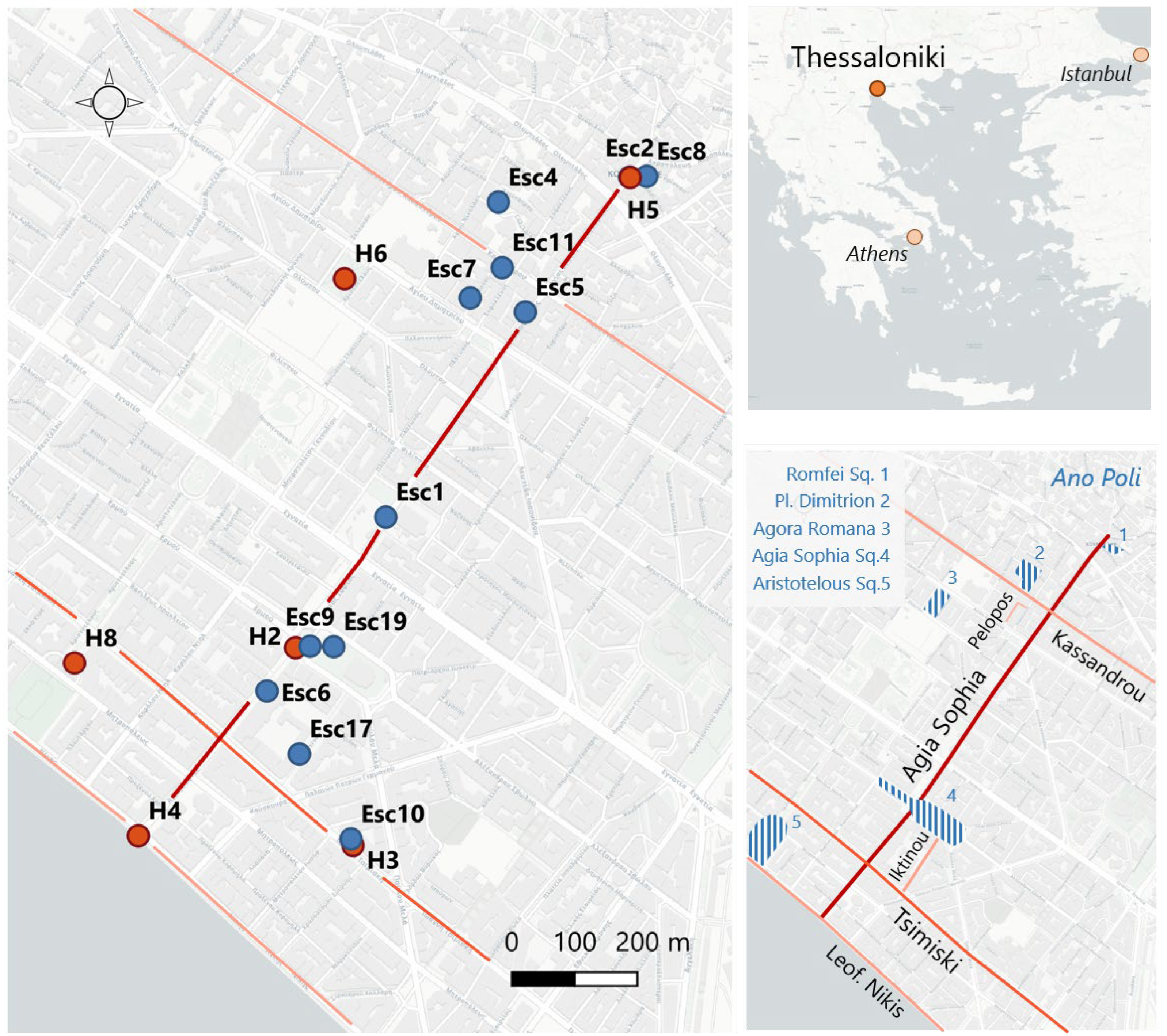
2.1. Case Study

The study area is located in the historic urban core of Thessaloniki, Greece (40.6401° N, 22.9444° E), along the northeastern coastline of the Thermaikos Gulf. Thessaloniki is the second largest city in Greece, with a municipal population of 317,778 and a metropolitan area population of approximately 1,011,000 [30]. The city serves as a key economic, cultural, and educational centre in the northern part of the country, with the Aristoteles University being the largest university in Greece. It is characterized by a densely built commercial centre and limited public open spaces and vegetation, with a comparatively low percentage of accessible green public space, with about 2.7 m² per capita [31], which is far below the recommended 9 m² benchmark suggested by the World Health Organization [32].

Thessaloniki is characterized by a complex orography, comprising extended flat areas in the west, north-west and the southern part of the greater Thessaloniki area, stretching over 20 km in a bowl formed by low hills facing a bay that opens into the Thermaikos Gulf. This complex coastal formation, in combination with the nearby mountainous areas from the northern to the eastern direction, favours various local circulation systems, such as sea–land breezes and valley–mountain winds, as well as wind-channelling phenomena [33]. The study area starts at near sea level (2 m a.s.l.) at the city’s seashore and rises along Agia Sophia road towards the Upper Town (Ano Poli).

The region has a typical Mediterranean climate, classified as CSa under the Köppen–Geiger climate classification system [34], with mild and wet winters and dry and hot summers, with significant seasonal temperature variation. The mean temperatures of Thessaloniki reach ~15.9 °C annually and ~23.96 °C for the hot season (May–September) [35]. Due to climate change, a continuous warming can be observed over the last decades. In summer, e.g., the number of desert days with maximum temperatures equal or above 35 °C within a year rose from 56 days (1983–1992) to 70 (1993–2002) and again to 141 days (2003–2012)—an increase of 152% from the first to the third decade [36]. Heatwaves, as prolonged periods of extreme thermal discomfort, are becoming a common phenomenon in Thessaloniki. A recent study projects a significant increase in the frequency of extreme heat stress, rising from about 8 heatwave days per year in the present climate to 20 days/year by 2050 and up to 60 days/year by 2100, with the duration extending by up to 30 days at maximum [35].

2.2. Measurement Campaign (DB)

Throughout the hot summer of July 2021, which was marked by several heatwaves, a micrometeorological measurement campaign was conducted in the city centre of Thessaloniki. The measuring setup consisted of twelve low-cost Escort Mini 2000 Temperature Loggers (Escort Data Logger Inc./Escort Messtechnik AG, Aesch by Birmernsdorf, Switzerland) measuring and recording every 30 min and six HOBO Pro v2 External Temperature/Relative Humidity Data Loggers (HOBO Data Loggers/LI-COR, Bourne, MA, USA) recording every 5 min. Before being used in the field, the sensors were tested in the lab at around 20 °C for functionality and any differences in measurement. The maximum deviation of the sensors was 0.2 °C and 2.5% relative humidity, thus remaining within the device-specific accuracy range (0.2 °C from 0 to 70 °C and 2.5% from 10 to 90% RH). The 18 data loggers were installed along a transect stretching from the seafront toward the historic old town of Ano Poli, primarily along Agia Sophia Street and sporadically in selected nearby streets. In coordination with the Thessaloniki city administration, the loggers were temporarily installed on streetlamps and poles at a height of 3 m, as well as on two balconies located on the top floors of the respective buildings. The location of the data logger, as well as the relevant streets and city squares, are illustrated in Figure 1.

The selected logger locations were intended to cover a wide range of thermal variance with regard to the following:

(1)

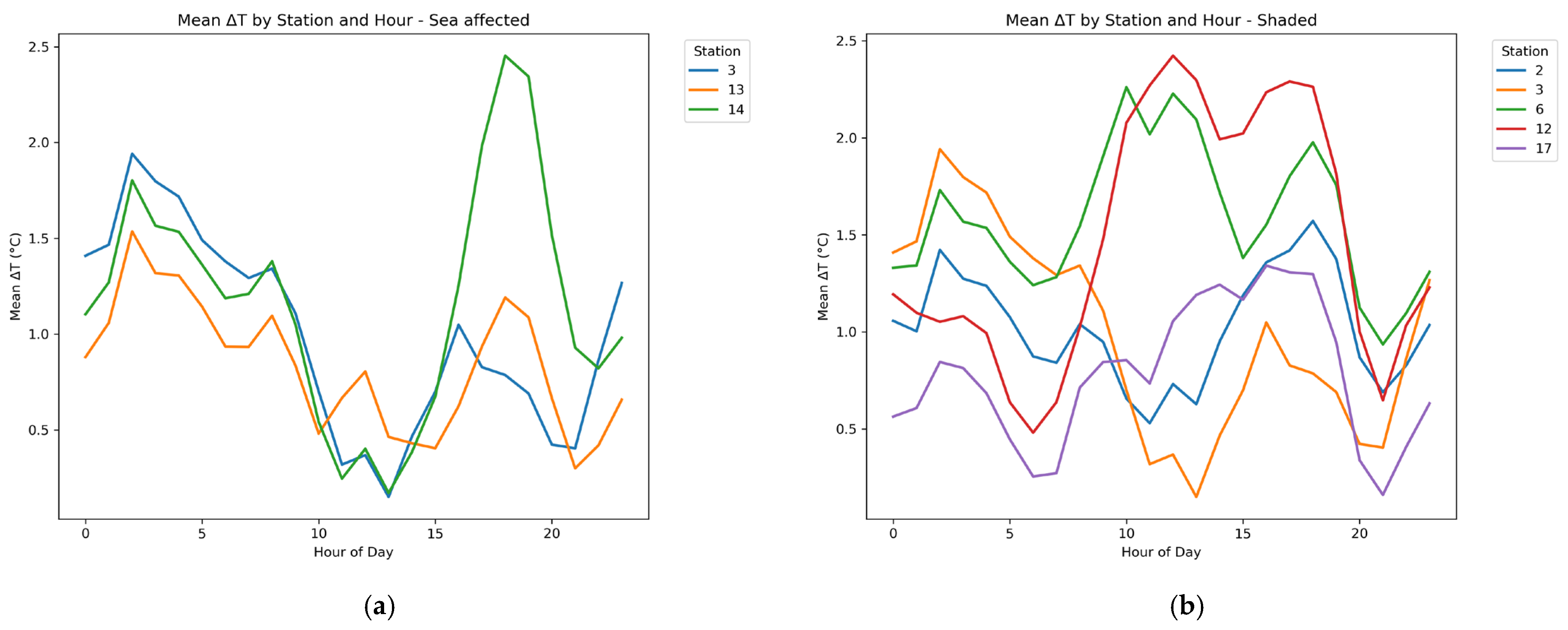
The effects of the sea and related ventilated areas versus poorly ventilated, densely built-up inner-city areas;

(2)

The effects of locations with nearly full solar radiation input versus locations with shading of different degrees:

a.

Building shade: streets with different orientations, street widths and the heights of adjacent buildings;

b.

Tree shade: varying street or park trees;

(3)

Warming effects caused by traffic: streets cover a wide range of traffic volumes, classified from major arterial road with heavy traffic volumes (Tsimiski) to local roads with primarily residential traffic and areas without traffic, such as pedestrian streets, parks, squares, and a courtyard.

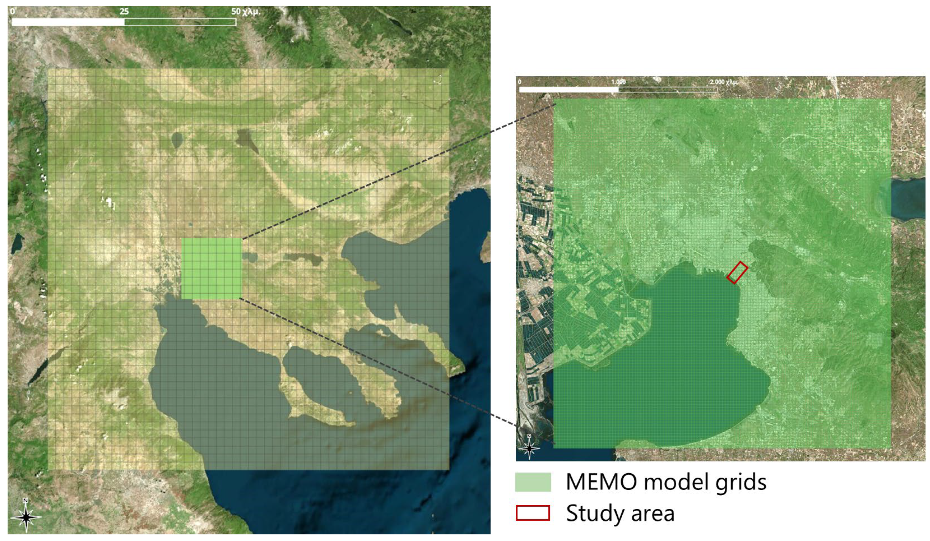
2.3. NWP and MEMO Model

NWP models have been used to study thermal effects in urban areas, as well as the influence of urban coverage on mesoscale and regional scale weather patterns. The MEMO model [37] has been applied and validated in a series of urban case studies, aiming to assess the model’s performance in predicting local dynamical and thermal effects [38,39] or provide high-resolution driving meteorology to a chemical dispersion model for air quality assessment [40]. In the latter case, MEMO has been used as the core meteorological module of an Operational Air Quality System, deployed as the official air quality assessment tool in Cyprus and as a tool for informing citizens of Thessaloniki on the current and next-day air quality situation.

In the present study, MEMO was used to simulate the meteorological situation in the local scale over the city of Thessaloniki during the month of July 2021, coinciding with a period of intense heatwaves. The model provided hourly 3D fields of temperature, relative humidity, wind speed and direction, and shortwave incoming radiation over an area of 30 × 30 km², covering the metropolitan area of Thessaloniki at a horizontal resolution of 250 m. A coarser model domain of 120 × 120 km² with a resolution of 4000 m was used to provide continuous boundary input to the high-resolution grid (Figure 2). Regional-scale input was incorporated in the nested model by forcing the coarse domain temperature and wind fields towards consistent fields generated based on radiosondes from the Macedonia airport [41], available at 6- or 12-hour intervals. The surface and radiation parameterizations used by MEMO for urban areas have been detailed and validated in Nitis et al. [38]. For the present application, a high-resolution map of surface types based on CORINE CLC2012 land use dataset [42] was used for the central areas of Thessaloniki.

Applying a mesoscale model over an urban area is expected to provide average thermal and radiative fields representing the local-scale situation and surface-induced effects, which are at best resolved at a scale of a few hundred meters. In this sense, the output fields obtained by the MEMO application are expected to represent corresponding spatial averages through areas of the size of a few city blocks, while smaller-scale shading or radiation-trapping effects are spatially smoothed out. Looking at the time series calculated by MEMO at the locations of deployed temperature sensors, it is evident that in most of the unshaded locations, the model underestimates the daily maxima. On the other hand, sensors in shaded locations indicated lower temperatures than those predicted by the model.

The effects of limited resolution become more pronounced in computational cells encompassing mixed land use. Typical examples include cells that contain water surfaces (e.g., near the coastline) where the average cell diurnal variation can significantly underestimate the extrema registered by adjacent land sensors. Cells that contain dense building structures with low porosity, e.g., with narrow street canyons separating contiguous building blocks, represent another case where the simplified, land use-based surface classification of the MEMO model can fail to represent the thermal response in sensors near the ground. Local variations in insolation penetration within a dense urban area are nearly impossible to resolve without an explicit 3D model, which further limits the accuracy of predicting radiation effects during the day.

Urbanization approaches, such as those proposed by Martilli et al., Salamanca et al., and Tsegas et al. [5,6,8], could potentially improve the performance of MEMO in capturing microclimatic features during datetime. However, these schemes heavily rely on the availability of additional datasets of high-resolution geometrical (3D structure, surface geometries, building silhouettes, etc.) and thermal properties (surface albedo, material properties, water permeability) that need to cover the entirety of the computational domain. Such data inventories are typically very hard to obtain in sufficient resolution and are usually characterized by a considerable amount of uncertainty. It has also been shown that the sensitivity of the urbanized parameterisations to input data uncertainties is still poorly understood [43]. In contrast, the computational scheme proposed in this work aims to augment thermal forecasts provided by the baseline model using only localized information that can be obtained by targeted surveys.

It is evident that not only unresolved subscale variations in urban surfaces, but also localized features of the sensor microenvironment, such as ventilation, shading, orientation, proximity to various surfaces and land cover types, can account for the observed bias between measurements and the local-scale model. In the subsequent sections, a machine-learning model is applied in an effort to further “downscale” the local-scale model fields by using specific features of each sensor microenvironment in combination with observed temperatures.

2.4. Random Forest Regression

Random Forest is a widely used machine learning model employed for both regression and classification tasks [44]. This type of model is based on the bagging of decision trees. Decision trees [45] are machine learning algorithms characterized by splitting nodes that represent decisions based on features, branches that connect the nodes and indicate the outcome of each decision, and leaves that provide the final prediction. In regression problems, the prediction is given as a numerical value.

Although decision trees are known for their simplicity and relatively low error, they tend to overfit the training dataset, which can lead to reduced model accuracy [46]. In general, a standalone decision tree is considered a weak learner [47]. To address this limitation, several methods have been proposed. Breiman et al. [45] introduced the bagging process (also known as bootstrap aggregation), an ensemble machine learning technique that combines multiple weak learners to create a stronger model. In bagging-based predictions, the outputs of several weak learners are averaged to improve performance. In Random Forest models, decision trees are used as weak learners, combined with both bagging and random feature selection [46].

Random Forest has been applied in various studies to predict environmental parameters associated with atmospheric conditions [11,14,15]. Moreover, many applications utilize datasets of atmospheric variables derived from numerical models [9,10], observational data, and other parameters relevant to the area of interest to train Random Forest models.

Since the primary objective of this study is to use Random Forest to explore the potential for temperature downscaling in an urban environment, from the local to the microscale, the features (the parameters utilized to train the model) used to train the model are analysed in detail in the following subsection.

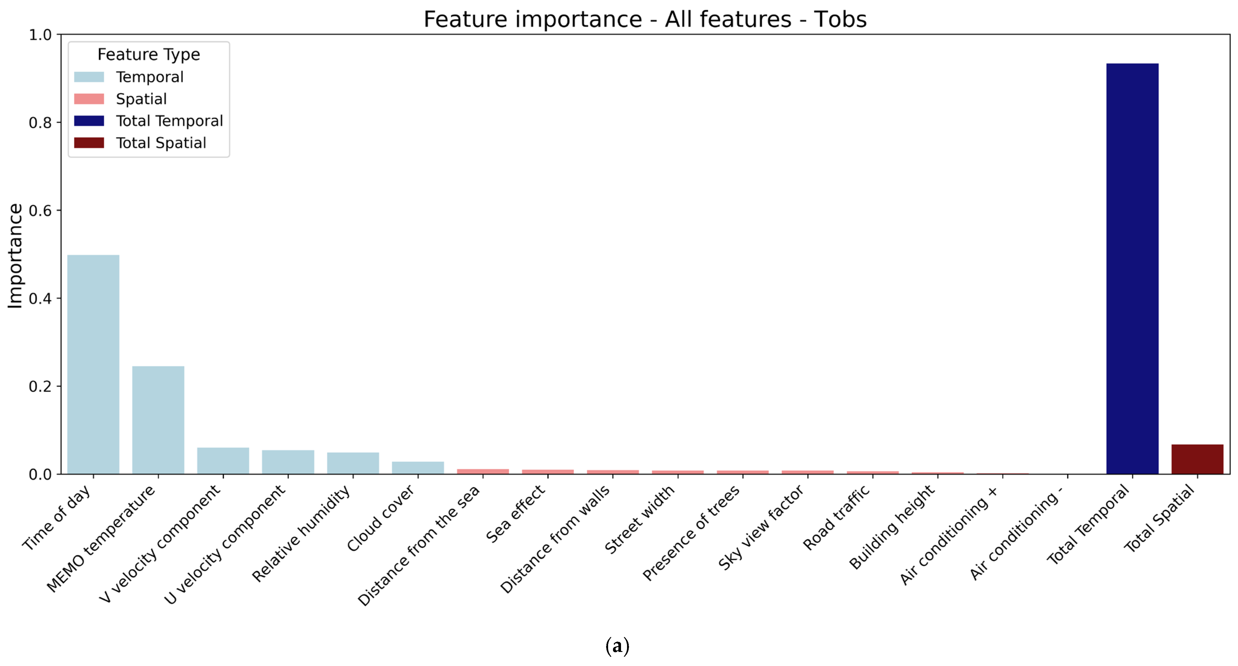
2.4.1. Feature Analysis

To assess the capability of downscaling temperature forecasts from the MEMO model, several Random Forest applications were conducted. Since temperature is a highly time-dependent variable, and this study also investigates the contribution of spatial characteristics to the downscaling process, two target variables were defined for prediction: the observed temperature $T_{obs}$, and the difference between the observed and the modelled temperature at each measurement station location, $\mathsf{\Delta }T$:

$$\mathsf{\Delta }T=T_{obs}-T_{mod}$$

(1)

where $T_{mod}$ is the temperature simulated from the MEMO model and $T_{obs}$ recorded by the low-cost sensor measurement network.

To train the Random Forest regression model, a variety of features were used, which can generally be categorized into two main groups:

• Time-dependent (“temporal”) features that are related to temporal characteristics, such as observed and modelled temperature data.
• Spatial-dependent (“spatial”) features that represent the geometric, topographic and thermal attributes of each location of interest.

Table 1. Features for the training of Random Forest regression model.

Training Dataset Features
Feature	Value	Type	Derived
Time of day	1–24 h
MEMO temperature	°C	temporal	Model
Relative humidity	0–100%	temporal	Model
$U$ velocity component	m/s	temporal	Model
$V$ velocity component	m/s	temporal	Model
Cloud cover	0–1	temporal	Measurement
Distance from the sea	m	spatial	Calculated
Distance from walls	m	spatial	Calculated
Street width	m	spatial	Calculated
Presence of trees	0–1	spatial	Estimated
Sky view factor	0–1	spatial	Calculated
Sea effect	0–1	spatial	Estimated
Building height	m	spatial	Calculated
Road traffic	0–1	spatial	Estimated
Air conditioning +	0–1	spatial	Estimated
Air conditioning −	0–1	spatial	Estimated

presents the features used to train the Random Forest regression model. For each feature, the type and data source are also indicated. The time of day represents the reference hour for both the measurements and the corresponding modelled data. The modelled features were obtained from the MEMO model at an hourly resolution. Similarly, observed temperature values were averaged to hourly intervals, along with cloud cover data, which was sourced from the Thessaloniki International Airport “Macedonia” meteorological station [41].

Spatial features and material properties that strongly affect temperature maxima inside urban canopies have been identified in many previous works. These typically include features connected to natural radiative and heat fluxes [48], including the presence of reflective surfaces, paved vs. permeable soil covers and proximity to vegetation and trees. Additional features, such as open vs. semi-open vs. enclosed geometries, are determining factors for ventilation efficiency and radiation trapping [49]. Finally, features describing proximity to large anthropogenic heat fluxes need to be considered [50,51]. In line with these established practices, ten spatial features have been selected for training the model: distance from the sea, distance from walls, street width, presence of trees, sky view factor, sea effect, building height, road traffic, air conditioning+, air conditioning−.

Table 2. Spatial parameters values for the 18 low-cost sensors.

Station	ID	Distance from the Sea (m)	Distance from Walls (m)	Street Width (m)	Presence of Trees	Sky View Factor	Sea Effect	Building Height	Road Traffic	Air Conditioning+	Air Conditioning−
1	Esc10	233	0.2	27	0	0.39	0.5	27	1	0	0
2	Esc17	275	8	19	1	0.4	0.5	13	0	0	0.5
3	Esc6	314	5	17	0.6	0.32	1	13	0	0	1
4	Esc9	414	15	223	0	0.83	0.5	13	0.6	0	0
5	Esc19	438	2	217	1	0.8	0	20	0	1	0
6	Esc1	649	3	74	0.3	0.47	0	5	0.6	0.5	0
7	Esc11	1073	2	14	0	0.28	0	17.5	1	0	0.5
8	Esc5	1042	1	12	0	0.12	0	16	0.6	1	0
9	Esc7	1001	0.2	6	0	0.57	0	14	0	0	0
10	Esc4	1152	1	6	0	0.4	0	14	0	0.5	0
11	Esc2	1310	1	9	0	0.16	0	15	0.3	0	0
12	Esc8	1337	5	59	0.6	0.39	0	14	0	0	0
13	H04	5	10	28	0	0.8	1	14	0.6	0	0
14	H08	157	3	31	0	0.49	1	18	0	0	0
15	H03	225	5	24	0.3	0.39	0	20	1	0	1
16	H02	397	10	112	0	0.77	0.5	20	0	0	0
17	H06	903	15	57	1	0.42	0.5	20	0	0	0
18	H05	1310	1	9	0	0.16	0	15	0.3	0	0.5

presents the values of these features for each of the 18 low-cost sensors. The distance from the sea and the distance from nearby walls for each station were calculated based on their geographic location within the city centre of Thessaloniki. The presence of trees, road traffic, and sea effects around each sensor location were estimated empirically and expressed on a scale from 0 to 1. Specifically, these empirically estimated spatial features were classified with values ranging from 0 to 1, in increments of 0.1. A value of 0 indicates the absence of the respective feature (e.g., no trees, no traffic, or no sea influence), while a value of 1 denotes strong presence or influence. Similarly, the influence of air conditioning systems near each sensor was estimated using two separate indicators:

• Air conditioning +: Indicates the impact of warm air from AC exhausts. A value of 1 signifies an AC exhaust in close proximity (up to 2 m) (Esc5), a value of 0.5 signifies AC exhausts in wider proximity (Esc1, Esc4). Esc 19 is a special case, influenced by the strong heating of a nearby sunlit wall.
• Air conditioning −: Represents the cooling effect of nearby AC systems. A value of 1 indicates a strong cooling effect on the sensors, which are located directly in front of the entrances to well-frequented, air-conditioned shops (H03, Esc6). A value of 0.5 indicates moderate effects of AC located approximately 3 to 5 m away or shops in less-frequented areas (H05, Esc2, Esc11, Esc17).

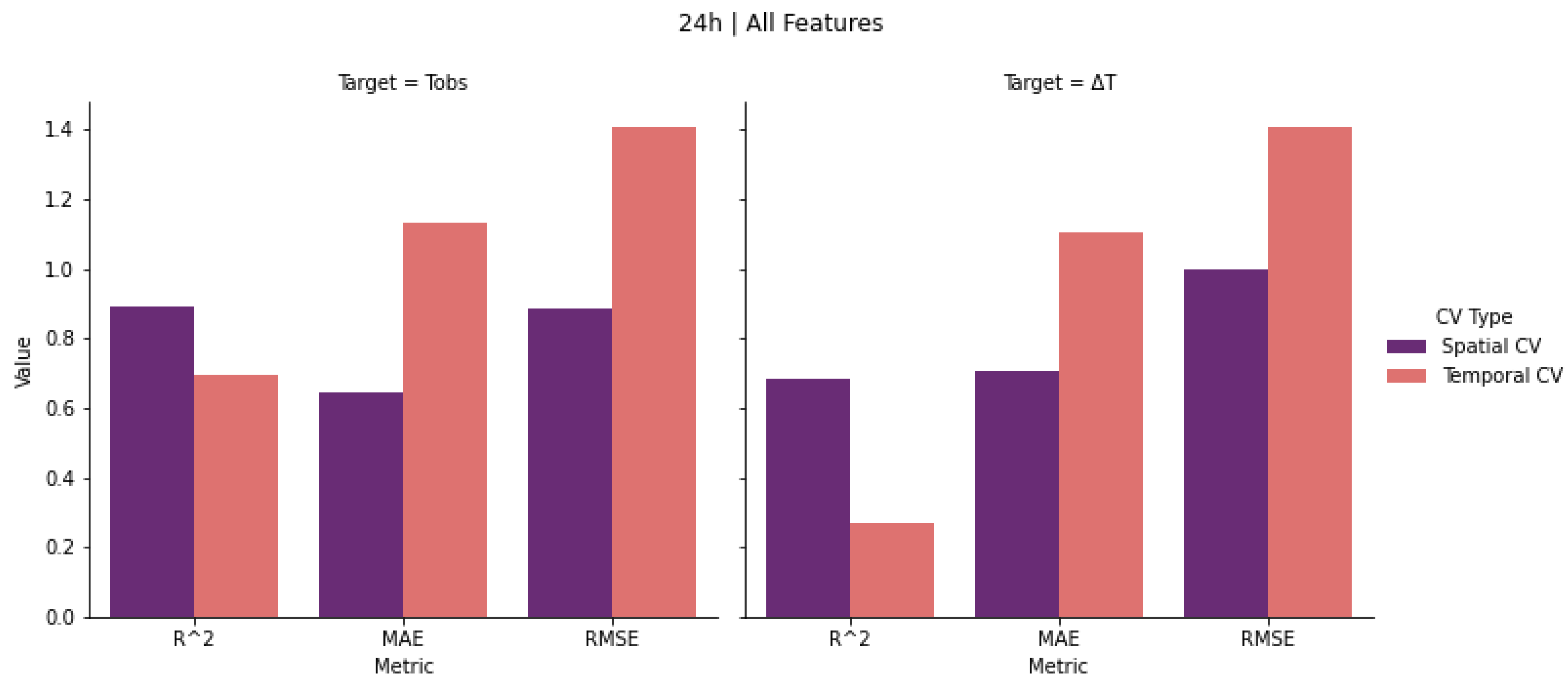
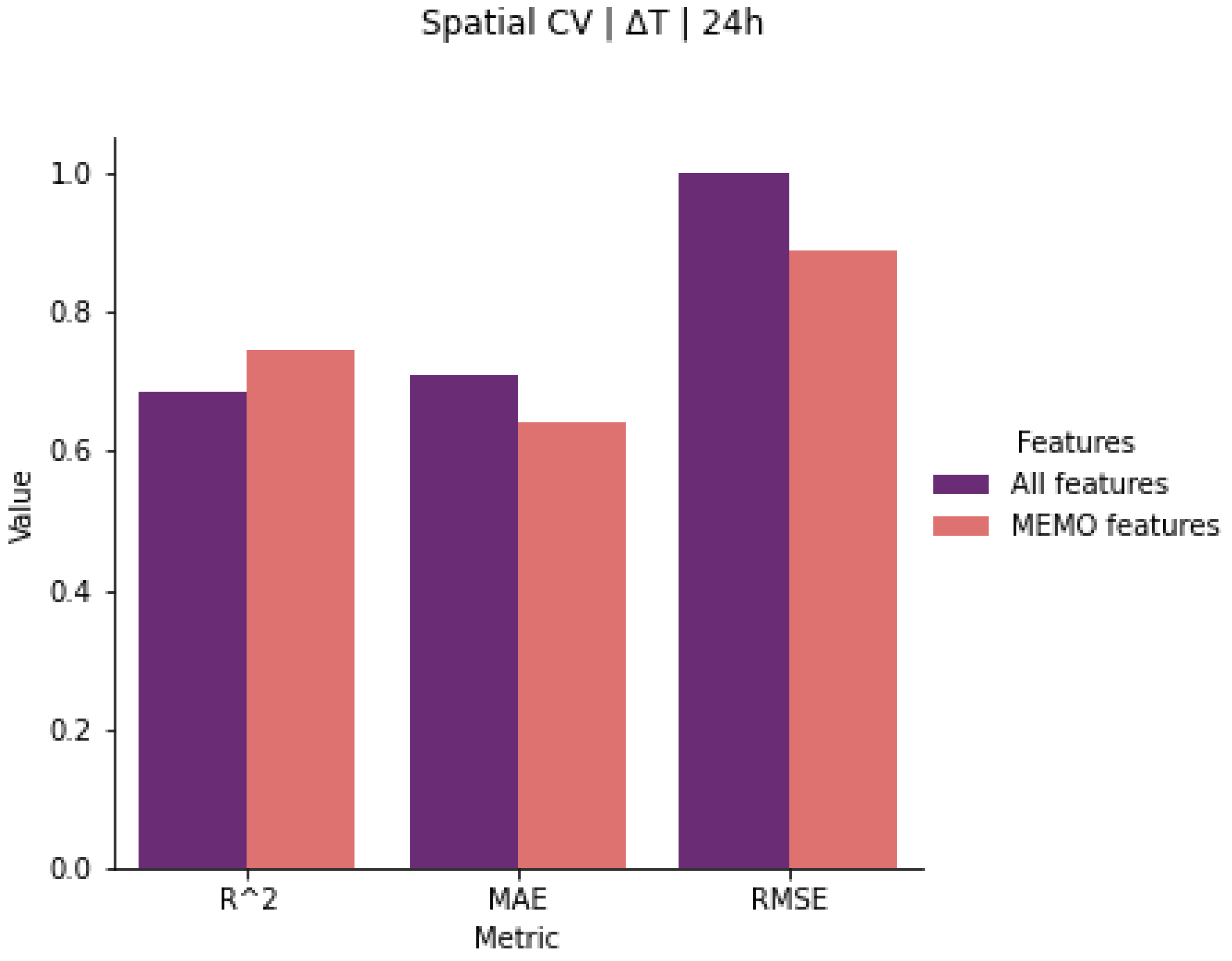
The Sky View Factor (SVF) was calculated using the SVF module in the SAGA Toolbox of QGIS, with the Digital Elevation Model (DEM) of Thessaloniki as input, with a resolution of 0.8 × 0.8 × 0.8 m³. This data was created from the “Very Large Scale Orthophtotos” (VLSO) project. The SVF ranges from 0 (completely obstructed sky) to 1 (completely open sky). Finally, the building height of the nearest structure to each sensor was estimated based on the number of building floors.

Table 2 presents the values of the 10 spatial features, as calculated or estimated for each of the 18 low-cost sensors.

2.4.2. Application

As mentioned in the previous subsection, this study aimed to evaluate the accuracy of Random Forest regression in predicting both $T_{obs}$ and $\mathsf{\Delta }T$ and to compare these predictions using different training datasets. To achieve this, multiple experiments were conducted using $T_{obs}$ and $\mathsf{\Delta }T$ as target variables. Initially, both target variables were predicted using the full set of features listed in Table 1. Separate runs were also performed using only the temporal features of the MEMO model. Furthermore, the results were evaluated by comparing models trained with all features across different time segments: the full 24 h period (“24 h” dataset), daytime (“Day” dataset) hours (08:00–20:00), and nighttime (“Night” dataset) hours (20:01–07:59).

Instead of using a fixed split between training and testing datasets, this study employed the cross-validation method. Cross-validation is an ensemble technique that partitions the dataset into multiple folds. Each fold is used as the test set once, while the remaining folds are used for training. Specifically, the dataset is divided into a predefined number of folds, and the model is trained and evaluated as many times as there are folds. The final results are obtained by averaging the performance metrics across all runs. Two types of cross-validation are used in this study:

• Spatial cross-validation (“Spatial CV”): a twelve-fold cross-validation where, in each fold, 3 out of the 18 sensor stations are left out for testing.
• Temporal cross-validation (“Temporal CV”): a twelve-fold cross-validation where, in each fold, 5 days of data are excluded from training and used for testing.

2.5. Evaluation Metrics

To evaluate the accuracy of each Random Forest model application, several standard regression metrics were used. Specifically, this study employed three of the most widely used evaluation metrics: the Coefficient of Determination ($R^2$), the Mean Absolute Error ($MAE$), and the Root Mean Squared Error ($RMSE$).

The Coefficient of Determination (Equation (2)) measures the proportion of variance in the target variable that can be explained by the input features. It provides insight into how well the model fits the data. An ideal model would yield an $R^2$ of 1. The metric is calculated using the following equation:

$$R^2={\displaystyle \frac{\sum _{i=1}^n{\left(y_i-\widehat{y_i}\right)}^2}{\sum _{i=1}^n{\left(y_i-\overline{y}\right)}^2}}$$

(2)

where $y_i$ is the actual target value for each prediction $i$, $\widehat{y_i}$ is the corresponding predicted value, $\overline{y}$ is the mean of the true values, and $n$ is the total number of samples.

The Mean Absolute Error (Equation (3)) quantifies the average magnitude of the errors between the predicted and actual values, without considering their direction. An ideal model would have an $MAE$ of 0. It is calculated as

$$MAE={\displaystyle \frac{1}{n}}{\sum }_{i=1}^n\left|y_i-\widehat{y_i}\right|$$

(3)

The Root Mean Squared Error (Equation (4)) measures the square root of the average squared differences between predicted and actual values. $RMSE$ is particularly sensitive to large errors and provides a good indication of the model’s performance when outliers are present. Similar to $MAE$, an ideal $RMSE$ is 0. It is defined as

$$RMSE=\sqrt{{\sum }_{i=1}^n{\displaystyle \frac{{(y_i-\widehat{y_i})}^2}{n}}}$$

(4)

3. Results

3.1. Comparing Mesoscale and Microscale Temperature on a Monthly Basis

Figure 3 and Figure 4 illustrate the temperature difference mean values for each hour of the day for the month of July 2021. The values shown are the $\mathsf{\Delta }T$ between the microscale stations (measured) minus the respective mesoscale (at local-scale resolution) MEMO model grid (modelled). For the exact location of the stations presented in Figure 3 and Figure 4, please refer to Figure 1 and Table 2 (station, ID).

Apart from station no. 5, all measured data are continuously warmer than the model, showing that the model underestimates temperatures at street scale by up to 5 °C. The strongest deviation from the model and largest variation between the stations occurs during the daytime, most probably due to differences in incoming solar radiation. While most stations exhibit greater positive deviations from the model during the day compared to nighttime, a few stations display the opposite behaviour, with reduced differences under daytime conditions, e.g., no. 3, 13, and 14 (see Figure 4a for a comparison). These specific stations are all close to the sea (see Figure 1 for a comparison: ID Esc6(3), H04(13), and H08(14)), making the sea’s cooling impact apparent during the day—in comparison to the mesoscale model.

At night, the temperature at street scale remains about 1 to 2 °C warmer than the model grid predicts, with only minor variations between the 18 stations. The low variability can be explained by the lack of differences in solar radiation input (high input leading to high temperatures) between the stations at night compared to the radiation-rich daytime. This also distinctively improves the performance of the mesoscale model, which by definition cannot account for radiation-induced differences at ground level. Persistently higher nighttime temperatures at the stations compared to the model indicate a direct UHI impact from heat-emitting buildings and sealed surfaces on the near-surface microclimatic measurements.

The larger discrepancies in MEMO’s temperature underestimation during the day indicate that the microclimatic effects of the urban environment during a heatwave are more difficult to capture with the MEMO model’s local-scale resolution (250 × 250 m²) during daytime hours. At the same time, while similar trends in ΔT values occur across all stations at night, the daytime variations in each station’s line highlight the influence of micro-environmental characteristics at different locations within the urban area.

In general, the measurements at street-scale strongly reflect the microclimatic effects of their nearby environment, showing distinct responses to changes in the measured air temperature. Temperature differences compared to the mesoscale model increase significantly in times of direct radiation input, which is even intensified as the station approaches a building façade or wall. In contrast, the delta between the stations’ data and the local-scale horizontal resolution model remains low during the day when the stations are shaded, or the sea breeze has a cooling effect.

Stations located in similar environmental settings are grouped in Figure 4 to illustrate the thermal effects of various influencing factors over the course of the day. The effects of shading (associated with reduced $\mathsf{\Delta }T$) and direct solar radiation (resulting in increased $\mathsf{\Delta }T$) is clearly evident. For instance, sensors positioned near the sea tend to record lower daytime temperature deviations (i.e., values closer to the model output) compared to nighttime, indicating a distinct cooling effect of maritime influence (station 3(Ecs6); 13(H04) in Figure 4a)). Conversely, a pronounced warming effect is observed at station 14 (H08), likely caused by solar radiation reflected from a nearby (2 to 3 m) façade during the afternoon hours.

The difference between the model and the stations shaded by trees remains relatively low (up to 2.4 °C) during the day (compare Figure 3 and Figure 4b), indicating a distinct cooling effect of trees on air temperature during the day. Daytime deviations between the shaded stations can be explained by their distance from the sea (the warmer stations no. 6 and 12 are located far away from the sea—649 m and 1337 m—compared to stations no. 2/3, which are 275 m and 314 m away) or the cooling effect of the surrounding park for station no. 17 (903 m from the sea).

Appendix A illustrates a matrix to provide a more detailed understanding of the correlation between $\mathsf{\Delta }T$ values across pairs of monitoring network stations. The correlation matrix highlights a general tendency for most stations to show increased deviations from the model during daytime, as reflected by predominantly positive correlation coefficients. Negative correlations, indicated in orange, are primarily associated with stations 3, 13, and 14, which exhibit a daytime cooling trend, as previously described.

3.2. Random Forest Regression Model

Figure 5 presents the evaluation metrics for the two target variables of interest, $T_{obs}$ and $\mathsf{\Delta }T$, for both spatial and temporal CVs, using the full 24 h dataset and all available features for training. The results clearly demonstrate that the spatial CV yields significantly better performance than temporal CV. Specifically, for both target variables, the $R^2$ values are higher under spatial CV, while the $MAE$ and $RMSE$ values are notably lower, indicating more accurate predictions from the Random Forest model when trained and tested using spatial partitions. Based on these findings, the following analyses focus exclusively on spatial CV applications. An additional observation from Figure 4 is that the model consistently performs better in predicting the observed temperature $T_{obs}$ compared to the temperature difference $\mathsf{\Delta }T$, suggesting that direct temperature measurements are easier for the model to estimate accurately than the residual errors between observed and modeled values.

The graph in Figure 6 shows the outcomes for the two target variables, as provided by the application of Random Forest using the 24 h, the Day, and the Night datasets for model training. As previously mentioned, only spatial CV was considered, and all features were included in the training process. The results show that the $R^2$ values remain relatively consistent across the three temporal subsets for both target variables. However, the $MAE$ and $RMSE$ values indicate that daytime (Day) predictions are less accurate. This is particularly evident during periods of extremely high temperatures and elevated $\mathsf{\Delta }T$ values at certain locations, which contributes to increased prediction errors in both targets. These daytime errors also influence the performance of the 24 h dataset, as it includes these challenging conditions. In contrast, predictions based on the nighttime (Night) dataset result in much lower $MAE$ and $RMSE$ values for both $T_{obs}$ and $\mathsf{\Delta }T$. This improvement is likely related to the urban heat island effect and the relatively stable nighttime temperatures observed in urban areas during heatwave events. During such conditions, nighttime temperatures do not drop significantly and often remain nearly constant until early morning. As also shown in Figure 2, the modelled–observed temperature difference $\mathsf{\Delta }T$ follows similar trends across all sensor locations, reinforcing the consistency of the model’s behaviour during nighttime.

Considering all the outcomes presented in the previous figures, it is important to examine the contribution of each feature to the prediction of both target variables, $T_{obs}$ and $\mathsf{\Delta }T$. Figure 7a,b illustrates the feature importance in the Random Forest model under spatial CV using the 24 h training dataset for the prediction of $T_{obs}$ (Figure 7a) and $\mathsf{\Delta }T$ (Figure 7b). In these graphs, temporal features are shown in blue, while spatial features are represented with red bars.

As it is shown in Figure 7a, the Random Forest model’s prediction of observed temperature $T_{obs}$ relies heavily on two features: time of day, which contributes nearly 50%, and MEMO temperature, contributing approximately 25%. These results are expected, given that temperature is inherently a time-dependent variable, following consistent diurnal patterns. However, the model assigns minimal importance to other temporal features and shows negligible reliance on spatial features for predicting $T_{obs}$. From this perspective, using the $T_{obs}$ variable as a target to downscale MEMO temperature data with the aim of capturing microscale spatial variability appears infeasible.

In contrast, Figure 7b presents the feature importance for the prediction of $\mathsf{\Delta }T$ (the difference between modelled and observed temperatures). Here, the contributions of time of day and MEMO temperature are reduced compared to the $T_{obs}$ case, while the importance of other temporal features increases. Most notably, this model demonstrates a significant increase in the involvement of spatial features. Specifically, 7 out of 10 spatial variables contribute approximately 2% each to the model’s training, with only building height and air conditioning effects showing negligible influence. This indicates that when using $\mathsf{\Delta }T$ as the target, the Random Forest model is more capable of incorporating spatial characteristics, such as urban geometry and topography, into its predictions. These features play a crucial role in capturing street-scale temperature variations, which are critical in investigating urban micro-climate effects.

The final graph, which compares the values of the evaluation metrics in different Random Forest applications, is presented in Figure 8. In that graph, the results of the models of $\mathsf{\Delta }T$ target for spatial CV are compared using the 24 h dataset for two cases. The first model was trained with all available features, while the second was trained using only features derived from the MEMO model. The results show a slightly better performance when using the MEMO model features in terms of evaluation metrics ($R^2$, $MAE$, and $RMSE$). However, the differences between the two approaches are relatively small. These findings are important for guiding the selection of spatial features in future applications, particularly in efforts to downscale MEMO model outputs to microscale urban environments and to further enhance the accuracy of Random Forest models.

4. Discussion

The present study focuses on investigating the potential for downscaling mesoscale temperature predictions from the MEMO model during an extreme heatwave event in an urban environment, using a Random Forest regression algorithm. For this purpose, hourly temperature measurements were collected from a monitoring network in the city centre of Thessaloniki, consisting of 18 low-cost sensors, during July 2021. These data were used to train and evaluate the Random Forest model. In addition, several temporal and spatial variables and characteristics were incorporated into the training process. The Random Forest algorithm was applied in different scenarios, which were compared using various datasets and cross-validation schemes. Two different target variables were used: the observed temperature, $T_{obs}$, and the difference between the observed and the modelled temperatures, $\mathsf{\Delta }T$.

Since this research field is relatively new; the current work incorporates some innovative elements that are not present in previous similar studies [18,19,20,21]. Most notably, it investigates how, and to what extent, spatial geometrical, morphological, and other urban characteristics contribute to the predictions of the machine learning algorithm. Moreover, this study proposes using $\mathsf{\Delta }T$, the difference between the measured temperature and the one modelled by the mesoscale model, instead of $T_{obs}$, as the target variable for temperature prediction. This approach is considered more suitable, as it avoids issues related to the high temporal variability of temperature and better captures microclimatic effects, which are particularly crucial during heatwave events. Furthermore, the growing use of low-cost sensors and Internet of Things (IoT) devices is expected to enhance the availability of observed temperature data within urban environments. In this context, utilizing a dataset from a dense, low-cost measurement network is highly important.

However, some assumptions and limitations are present in this study. First and foremost, both the modelled and observed datasets cover only a single month, which includes multiple heatwaves in a single urban area (the city centre of Thessaloniki). To mitigate the risk of overfitting, the model was trained using hourly temperature data rather than daily mean, maximum, or minimum temperatures, and the maximum number of available sensors was employed. It should be noted that the proposed methodology should be evaluated in other urban environments and with datasets that include a greater number of extreme heatwave events. The authors are currently exploring the potential availability of such data to assess the general applicability and accuracy of the methodology. Another limitation is that only the Random Forest algorithm was used for downscaling MEMO model temperature predictions. As discussed in the introduction, there is no consensus in the literature on a universally superior machine learning algorithm for this type of problem. Thus, evaluating multiple algorithms was beyond the scope of the present study. However, a comprehensive comparison of several algorithms’ accuracy is planned for future work, using the current case study and dataset. Finally, feature selection in this study was guided either by literature-based practices or by the authors’ experience and knowledge of the specific characteristics of Thessaloniki’s city centre. Spatially dependent features and their classification were handled as described in Section 2.4.1. It should be noted that a future analysis of spatial feature selection is planned, using machine learning techniques such as feature engineering.

Improving the downscaling of mesoscale model outputs through the incorporation of local measurements represents a crucial advancement toward more accurate representations of urban microclimates. Such improvements are particularly relevant for future urban planning strategies related to climate adaptation, to identify priority neighbourhoods of excessive heat [24,52]. While the approach demonstrates promising results, the current stage of development does not yet provide the level of robustness required for administrative planning processes. Reliable, high-resolution data remain a prerequisite for evidence-based decision-making in this context so far.

Nonetheless, the measurement results reinforce existing knowledge regarding factors influencing urban microclimates at the local scale. For example, Figure 4a showed a distinct cooling effect for stations with direct access to the sea breeze [53], and 4b illustrates the localized cooling effect of a small inner-city park on near-surface air temperature. In addition, the results showed a distinct cooling effect of street trees on air temperature (and of course thermal comfort, which was not analysed in this study), in line with the current state of research [54]. Given Thessaloniki’s notable scarcity of green and vegetated spaces, these findings underscore the necessity for urban planning efforts to prioritize the expansion of park areas and other types of green infrastructure as an essential climate adaptation strategy [52].

The monthly mean $\mathsf{\Delta }T$ values indicate that, in general, the MEMO model underestimates urban temperatures compared to the sensor recordings. This underestimation becomes significantly more pronounced during the daytime, with a maximum monthly mean $\mathsf{\Delta }T$ of 5 °C observed (Figure 3). In contrast, nighttime $\mathsf{\Delta }T$ values are lower, typically ranging between 1 and 2 °C. Furthermore, while $\mathsf{\Delta }T$ trends are similar across all stations at night, daytime curves vary considerably between stations, as shown in Figure 3. This suggests that the microclimatic characteristics of different urban locations are much more difficult to capture by the MEMO model during the daytime than at night. Further analysis, illustrated in Figure 4, reveals that stations sharing similar spatial characteristics (e.g., affected by the sea or located in a shady location) tend to exhibit similar $\mathsf{\Delta }T$ trends. Therefore, it is crucial to investigate how such spatial characteristics can be integrated into the Random Forest model, and at what stage they contribute most effectively to its performance.

The results of the Random Forest model applied across different scenarios provide several insights. As shown in Figure 6, when the model is trained using three distinct 24 h based datasets (“24 h,” “Day,” and “Night”), the $R^2$ values remain relatively similar across all three scenarios. However, both $MAE$ and $RMSE$ errors are significantly higher for the “Day” dataset and much lower for the “Night” dataset. These findings apply to both $T_{obs}$ and $\mathsf{\Delta }T$ target variables and are consistent with the greater discrepancies observed in the MEMO model’s predictions during the daytime (Figure 3). Therefore, except for the results described in Section 3.1, which show that the MEMO model’s performance is influenced by street-scale microclimatic characteristics during daytime, the accuracy of the Random Forest model (trained on both MEMO and measured data) also declines during the hours of the day for the same reasons.

Figure 5 clearly shows that the spatial CV approach provides significantly better predictions than the temporal CV, which demonstrates very low accuracy for both target variables, $T_{obs}$ and $\mathsf{\Delta }T$. In particular, the $R^2$ metric reaches nearly 0.9 for the $T_{obs}$ target and approximately 0.7 for $\mathsf{\Delta }T$ under the spatial CV scheme. Although this indicates a notable difference in the accuracy of the Random Forest model, further analysis of feature importance for each target variable reveals an interesting insight: when $T_{obs}$ is used as the target, spatial characteristics contribute only marginally to the predictions. Daily temperature is inherently time-dependent, typically following consistent 24 h patterns.

To assess the quality of the predictions provided, it is useful to compare the evaluation metrics with those reported in previous studies. In the work by Shi and Yi [21], where $\mathsf{\Delta }T$ was also used to downscale hourly temperatures for four months (July and August of 2016 and 2017) in Seoul, during which several heatwave events were observed, the $RMSE$ for hourly predictions ranged from 1.36 to 1.51 °C. In contrast, the present work achieves better accuracy, with a corresponding $RMSE$ of approximately 1 °C when using all features, as shown in Figure 8. In another study by Blunn et al. [20], which also used $\mathsf{\Delta }T$ as the target variable, very high accuracy was reported, with $MAE$ values ranging from 0.15 to 0.2 °C. In contrast, the corresponding $MAE$ in the present study is approximately 0.65 °C. It is important to note, however, that Blunn et al. performed temperature downscaling at a 100 m resolution with a subsequent averaging of local extrema, not at the street-scale level used in the present work.

As shown in Figure 7a, nearly 75% of the predictive power comes from just two temporal features: time of the day and MEMO temperature. In this case, the contribution of spatial features is negligible. In contrast, when $\mathsf{\Delta }T$ is used as the target variable, the importance of temporal features decreases, while spatial features play a much more significant role in the Random Forest model’s predictions (Figure 7b). These findings are valuable in the context of applying machine learning for downscaling NWP temperature outputs, as they emphasize the crucial role of spatial characteristics in micro-scale environments. From this perspective, using $\mathsf{\Delta }T$ as the target variable aligns more closely with the goal of this study.

However, future research should focus on improving the accuracy of the machine learning methodology. To achieve this, we recommend deploying denser low-cost monitoring networks, increasing the availability of observational time series during heatwaves, applying the methodology in different urban areas, implementing the methodology using other machine learning algorithms, evaluating their performance, and exploring spatial feature selections by utilizing feature engineering techniques to enhance the training process.

5. Conclusions

In the current study, it was found that, in general, the mesoscale model MEMO, even when applied at a very high local-scale resolution (250 × 250 m²), struggles to capture the microclimate of the urban environment during a heatwave, especially during the daytime. The application of Random Forest shows potential for downscaling the MEMO model to a microscale for temperature prediction. For this purpose, the Random Forest model was trained using temporal and spatial features to incorporate both time-dependent factors and urban geometry characteristics into the predictions. The findings indicate that using spatial CV significantly increases the accuracy of Random Forest estimations. Moreover, using the difference between observed and modelled temperatures ($\mathsf{\Delta }T$) as the target variable is a more appropriate method for incorporating street-scale spatial characteristics into the predictions. However, further research is needed, using larger datasets from multiple heatwave events in different areas, utilizing several machine learning algorithms, and examining spatial feature selection and tuning methods to explore the potential for improving model accuracy.

References

1. Chen, F.; Dudhia, J. Coupling an Advanced Land Surface–Hydrology Model with the Penn State–NCAR MM5 Modeling System. Part I: Model Implementation and Sensitivity. Mon. Weather Rev. 2001, 129, 569–585. [Google Scholar] [CrossRef]
2. Grimmond, C.S.B.; Blackett, M.; Best, M.J.; Barlow, J.; Baik, J.J.; Belcher, S.E.; Bohnenstengel, S.I.; Calmet, I.; Chen, F.; Dandou, A.; et al. The International Urban Energy Balance Models Comparison Project: First Results from Phase 1. J. Appl. Meteorol. Climatol. 2010, 49, 1268–1292. [Google Scholar] [CrossRef]
3. Masson, V. A Physically-Based Scheme for the Urban Energy Budget in Atmospheric Models. Bound. Layer Meteorol. 2000, 94, 357–397. [Google Scholar] [CrossRef]
4. Kusaka, H.; Kimura, F. Coupling a Single-Layer Urban Canopy Model with a Simple Atmospheric Model: Impact on Urban Heat Island Simulation for an Idealized Case. J. Meteorol. Soc. Jpn. Ser. II 2004, 82, 67–80. [Google Scholar] [CrossRef]
5. Salamanca, F.; Krpo, A.; Martilli, A.; Clappier, A. A New Building Energy Model Coupled with an Urban Canopy Parameterization for Urban Climate Simulations—Part I. Formulation, Verification, and Sensitivity Analysis of the Model. Theor. Appl. Climatol. 2010, 99, 331–344. [Google Scholar] [CrossRef]
6. Martilli, A.; Clappier, A.; Rotach, M.W. An Urban Surface Exchange Parameterisation for Mesoscale Models. Bound. Layer Meteorol. 2002, 104, 261–304. [Google Scholar] [CrossRef]
7. Krayenhoff, E.S.; Voogt, J.A. A Microscale Three-Dimensional Urban Energy Balance Model for Studying Surface Temperatures. Bound. Layer Meteorol. 2007, 123, 433–461. [Google Scholar] [CrossRef]
8. Tsegas, G.; Moussiopoulos, N.; Barmpas, F.; Akylas, V.; Douros, I. An Integrated Numerical Methodology for Describing Multiscale Interactions on Atmospheric Flow and Pollutant Dispersion in the Urban Atmospheric Boundary Layer. J. Wind. Eng. Ind. Aerodyn. 2015, 144, 191–201. [Google Scholar] [CrossRef]
9. de Burgh-Day, C.O.; Leeuwenburg, T. Machine Learning for Numerical Weather and Climate Modelling: A Review. Geosci. Model Dev. 2023, 16, 6433–6477. [Google Scholar] [CrossRef]
10. Bochenek, B.; Ustrnul, Z. Machine Learning in Weather Prediction and Climate Analyses—Applications and Perspectives. Atmosphere 2022, 13, 180. [Google Scholar] [CrossRef]
11. Meenal, R.; Michael, P.A.; Pamela, D.; Rajasekaran, E. Weather Prediction Using Random Forest Machine Learning Model. Indones. J. Electr. Eng. Comput. Sci. 2021, 22, 1208–1215. [Google Scholar] [CrossRef]
12. Goutham, N.; Alonzo, B.; Dupré, A.; Plougonven, R.; Doctors, R.; Liao, L.; Mougeot, M.; Fischer, A.; Drobinski, P. Using Machine-Learning Methods to Improve Surface Wind Speed from the Outputs of a Numerical Weather Prediction Model. Bound. Layer Meteorol. 2021, 179, 133–161. [Google Scholar] [CrossRef]
13. Shin, J.-Y.; Min, B.; Kim, K.R. High-Resolution Wind Speed Forecast System Coupling Numerical Weather Prediction and Machine Learning for Agricultural Studies—A Case Study from South Korea. Int. J. Biometeorol. 2022, 66, 1429–1443. [Google Scholar] [CrossRef]
14. Das, S.; Chakraborty, R.; Maitra, A. A Random Forest Algorithm for Nowcasting of Intense Precipitation Events. Adv. Space Res. 2017, 60, 1271–1282. [Google Scholar] [CrossRef]
15. Yao, H.; Li, X.; Pang, H.; Sheng, L.; Wang, W. Application of Random Forest Algorithm in Hail Forecasting over Shandong Peninsula. Atmos. Res. 2020, 244, 105093. [Google Scholar] [CrossRef]
16. Vlachokostas, C.; Banias, G.; Athanasiadis, A.; Achillas, C.; Akylas, V.; Moussiopoulos, N. Cense: A Tool to Assess Combined Exposure to Environmental Health Stressors in Urban Areas. Environ. Int. 2014, 63, 1–10. [Google Scholar] [CrossRef]
17. Powell, J.P.; Reinhard, S. Measuring the Effects of Extreme Weather Events on Yields. Weather. Clim. Extrems 2016, 12, 69–79. [Google Scholar] [CrossRef]
18. Chajaei, F.; Bagheri, H. Machine Learning Framework for High-Resolution Air Temperature Downscaling Using LiDAR-Derived Urban Morphological Features. Urban Clim. 2024, 57, 102102. [Google Scholar] [CrossRef]
19. Bhakare, S.; Dal Gesso, S.; Venturini, M.; Zardi, D.; Trentini, L.; Matiu, M.; Petitta, M. Intercomparison of Machine Learning Models for Spatial Downscaling of Daily Mean Temperature in Complex Terrain. Atmosphere 2024, 15, 1085. [Google Scholar] [CrossRef]
20. Blunn, L.P.; Ames, F.; Croad, H.L.; Gainford, A.; Higgs, I.; Lipson, M.; Lo, C.H.B. Machine Learning Bias Correction and Downscaling of Urban Heatwave Temperature Predictions from Kilometre to Hectometre Scale. Meteorol. Appl. 2024, 31, e2200. [Google Scholar] [CrossRef]
21. Shin, Y.; Yi, C. Statistical Downscaling of Urban-Scale Air Temperatures Using an Analog Model Output Statistics Technique. Atmosphere 2019, 10, 427. [Google Scholar] [CrossRef]
22. Yang, S.; Wang, L.L.; Stathopoulos, T. A Review of Recent Progress on Urban Microclimate Research. In Proceedings of the 5th International Conference on Building Energy and Environment, Montréal, QC, Canada, 25–29 July 2022; Wang, L.L., Ge, H., Zhai, Z.J., Qi, D., Ouf, M., Sun, C., Wang, D., Eds.; Environmental Science and Engineering. Springer: Singapore, 2023; pp. 3029–3038, ISBN 978-981-19-9821-8. [Google Scholar]
23. Venter, Z.S.; Brousse, O.; Esau, I.; Meier, F. Hyperlocal Mapping of Urban Air Temperature Using Remote Sensing and Crowdsourced Weather Data. Remote Sens. Environ. 2020, 242, 111791. [Google Scholar] [CrossRef]
24. Gallacher, C.; Boehnke, D. Pedestrian Thermal Comfort Mapping for Evidence-Based Urban Planning; an Interdisciplinary and User-Friendly Mobile Approach for the Case Study of Dresden, Germany. Int. J. Biometeorol. 2025. [Google Scholar] [CrossRef]
25. Varnakovida, P.; Ko, H.Y.K. Urban Expansion and Urban Heat Island Effects on Bangkok Metropolitan Area in the Context of Eastern Economic Corridor. Urban Clim. 2023, 52, 101712. [Google Scholar] [CrossRef]
26. ZhanZhang, M.; Yiğit, İ.; Adigüzel, F.; Hu, C.; Chen, E.; Siyavuş, A.E.; Elmastaş, N.; Ustuner, M.; Kaya, A.Y. Impact of Urban Surfaces on Microclimatic Conditions and Thermal Comfort in Burdur, Türkiye. Atmosphere 2024, 15, 1375. [Google Scholar] [CrossRef]
27. Zheng, S.; Chen, X.; Liu, Y. Impact of Urban Renewal on Urban Heat Island: Study of Renewal Processes and Thermal Effects. Sustain. Cities Soc. 2023, 99, 104995. [Google Scholar] [CrossRef]
28. Boehnke, D.; Jehling, M.; Vogt, J. What Hinders Climate Adaptation? Approaching Barriers in Municipal Land Use Planning through Participant Observation. Land Use Policy 2023, 132, 106786. [Google Scholar] [CrossRef]
29. Grimmond, S.; Ward, H.C. Urban Measurements and Their Interpretation. In Springer Handbook of Atmospheric Measurements; Foken, T., Ed.; Springer Handbooks; Springer International Publishing: Cham, Switzerland, 2021; pp. 1391–1423. ISBN 978-3-030-52170-7. [Google Scholar]
30. Hellenic Statistical Authority Population and Housing Census. Available online: https://www.ktimanet.gr/geoportal/catalog/search/resource/details.page?uuid=%7BDF5B1140-D957-4678-8C50-2B66066D227B%7D (accessed on 10 July 2025).
31. Sylliris, N.; Papagiannakis, A.; Vartholomaios, A. Improving the Climate Resilience of Urban Road Networks: A Simulation of Microclimate and Air Quality Interventions in a Typology of Streets in Thessaloniki Historic Centre. Land 2023, 12, 414. [Google Scholar] [CrossRef]
32. World Health Organization. Urban Green Spaces: A Brief for Action; World Health Organization: Geneva, Switzerland, 2017. [Google Scholar]
33. Moussiopoulos, N.; Vlachokostas, C.; Tsilingiridis, G.; Douros, I.; Hourdakis, E.; Naneris, C.; Sidiropoulos, C. Air Quality Status in Greater Thessaloniki Area and the Emission Reductions Needed for Attaining the EU Air Quality Legislation. Sci. Total Environ. 2009, 407, 1268–1285. [Google Scholar] [CrossRef]
34. Kottek, M.; Grieser, J.; Beck, C.; Rudolf, B.; Rubel, F. World Map of the Köppen-Geiger Climate Classification Updated. Meteorol. Z. 2006, 15, 259–263. [Google Scholar] [CrossRef]
35. Papadopoulos, G.; Keppas, S.C.; Parliari, D.; Kontos, S.; Papadogiannaki, S.; Melas, D. Future Projections of Heat Waves and Associated Mortality Risk in a Coastal Mediterranean City. Sustainability 2024, 16, 1072. [Google Scholar] [CrossRef]
36. Slini, T.; Papakostas, K.T. 30 Years Air Temperature Data Analysis in Athens and Thessaloniki, Greece. In Energy, Transportation and Global Warming; Springer: Cham, Switzerland, 2016; pp. 21–33. [Google Scholar]
37. Moussiopoulos, N. The EUMAC Zooming Model, a Tool for Local-to-Regional Air Quality Studies. Meteorol. Atmos. Phys. 1995, 57, 115–133. [Google Scholar] [CrossRef]
38. Nitis, T.; Tsegas, G.; Moussiopoulos, N.; Gounaridis, D. Assimilating Anthropogenic Heat Flux Estimated from Satellite Data in a Mesoscale Flow Model. In Proceedings of the Air Pollution Modeling and Its Application XXV 35, Chania, Greece, 3–7 October 2016; 2018; pp. 219–224. [Google Scholar]
39. Moussiopoulos, N.; Douros, I.; Louka, P.; Simonidis, C.; Arvanitis, A. Evaluation of MEMO Using the ESCOMPTE Pre-Campaign Dataset. In Proceedings of the 8th International Conference on Harmonisation Within Atmospheric Dispersion Modelling for Regulatory Purposes Proceedings, Sofia, Bulgaria, 14–17 October 2002; p. 87. [Google Scholar]
40. Moussiopoulos, N.; Douros, I.; Tsegas, G.; Kleanthous, S.; Chourdakis, E. An Air Quality Management System for Policy Support in Cyprus. Adv. Meteorol. 2012, 2012, 959280. [Google Scholar] [CrossRef]
41. WMO 16622 “Macedonia” Airport Meteorological Station. Available online: https://rp5.ru/Weather_in_Thessaloniki_(airport) (accessed on 10 July 2025).
42. Büttner, G. CORINE Land Cover and Land Cover Change Products. In Land Use and Land Cover Mapping in Europe: Practices & Trends; Springer: Berlin/Heidelberg, Germany, 2014; pp. 55–74. [Google Scholar]
43. Buccolieri, R.; Santiago, J.L.; Martilli, A. CFD Modelling: The Most Useful Tool for Developing Mesoscale Urban Canopy Parameterizations. Build. Simul. 2021, 14, 407–419. [Google Scholar] [CrossRef]
44. Breiman, L. Random Forests. Mach. Learn. 2001, 45, 5–32. [Google Scholar] [CrossRef]
45. Breiman, L.; Friedman, J.; Olshen, R.A.; Stone, C.J. Classification and Regression Trees; Routledge: London, UK, 2017. [Google Scholar]
46. Sekulić, A.; Kilibarda, M.; Heuvelink, G.; Nikolić, M.; Bajat, B. Random Forest Spatial Interpolation. Remote Sens. 2020, 12, 1687. [Google Scholar] [CrossRef]
47. Xia, L.-G. Understanding the Boosted Decision Tree Methods with the Weak-Learner Approximation. arXiv 2018. [Google Scholar] [CrossRef]
48. Matzarakis, A.; Rutz, F.; Mayer, H. Modelling Radiation Fluxes in Simple and Complex Environments: Basics of the RayMan Model. Int. J. Biometeorol. 2010, 54, 131–139. [Google Scholar] [CrossRef]
49. Buccolieri, R.; Hang, J. Recent Advances in Urban Ventilation Assessment and Flow Modelling. Atmosphere 2019, 10, 144. [Google Scholar] [CrossRef]
50. Krpo, A.; Salamanca, F.; Martilli, A.; Clappier, A. On the Impact of Anthropogenic Heat Fluxes on the Urban Boundary Layer: A Two-Dimensional Numerical Study. Bound. Layer Meteorol. 2010, 136, 105–127. [Google Scholar] [CrossRef]
51. Grajeda-Rosado, R.M.; Alonso-Guzmán, E.M.; Pozo, C.E.-D.; Esparza-López, C.J.; Sotelo-Salas, C.; Martínez-Molina, W.; Mondragon-Olan, M.; Cabrera-Macedo, A. Anthropogenic Vehicular Heat and Its Influence on Urban Planning. Atmosphere 2022, 13, 1259. [Google Scholar] [CrossRef]
52. Norton, B.A.; Coutts, A.M.; Livesley, S.J.; Harris, R.J.; Hunter, A.M.; Williams, N.S.G. Planning for Cooler Cities: A Framework to Prioritise Green Infrastructure to Mitigate High Temperatures in Urban Landscapes. Landsc. Urban Plan. 2015, 134, 127–138. [Google Scholar] [CrossRef]
53. He, B.-J.; Ding, L.; Prasad, D. Relationships among Local-Scale Urban Morphology, Urban Ventilation, Urban Heat Island and Outdoor Thermal Comfort under Sea Breeze Influence. Sustain. Cities Soc. 2020, 60, 102289. [Google Scholar] [CrossRef]
54. Wong, N.H.; Tan, C.L.; Kolokotsa, D.D.; Takebayashi, H. Greenery as a Mitigation and Adaptation Strategy to Urban Heat. Nat. Rev. Earth Environ. 2021, 2, 166–181. [Google Scholar] [CrossRef]
Figure 1. Location of the 18 data loggers (Escort loggers in blue and HOBO loggers in red) along Agia Sophia Street in Thessaloniki, Greece. Map source: http://basemaps.cartocdn.com, accessed on 3 May 2025.
Atmosphere 16 00877 g001
Figure 2. Coarse (left) and fine (right) computational grids used by the MEMO mesoscale model, as well as the study area where the 18 measurement stations were temporarily installed.
Atmosphere 16 00877 g002
Figure 3. Average diurnal profiles of the difference between the MEMO-modelled and observed temperatures, Δ T , for the 18 low-cost measurement sensors.
Atmosphere 16 00877 g003
Figure 4. Examples of average diurnal profiles of the differences between the MEMO-modelled and observed temperatures, Δ T , are shown for the low-cost sensors located in sea-affected sites (a) and tree-shaded spaces (b).
Atmosphere 16 00877 g004
Figure 5. The R 2 , M A E and R M S E values for the two target variables, T o b s and Δ T , for both spatial and temporal CVs, using the full 24 h dataset and all available features for training.
Atmosphere 16 00877 g005
Figure 6. The R 2 , M A E and R M S E values for the two target variables, T o b s and Δ T , for both the 24 h, the Day and the Night datasets, using spatial CV and all available features for training.
Atmosphere 16 00877 g006
Figure 7. Feature importance in the Random Forest model using all features, spatial CV, and the 24 h dataset for predicting T o b s (a) and Δ T (b). Temporal features are shown in blue, while spatial features are represented with red bars.
Atmosphere 16 00877 g007aAtmosphere 16 00877 g007b
Figure 8. The R 2 , M A E , and R M S E values for the two target variables, T o b s and Δ T , for both the 24 h, the Day, and the Night datasets, using spatial CV and all available features for training.
Atmosphere 16 00877 g008