


Assessing the Cooling Effects of Water Bodies Based on Urban Environments: Case Study of Dianchi Lake in Kunming, China

Abstract
1. Introduction
2. Data and Methods
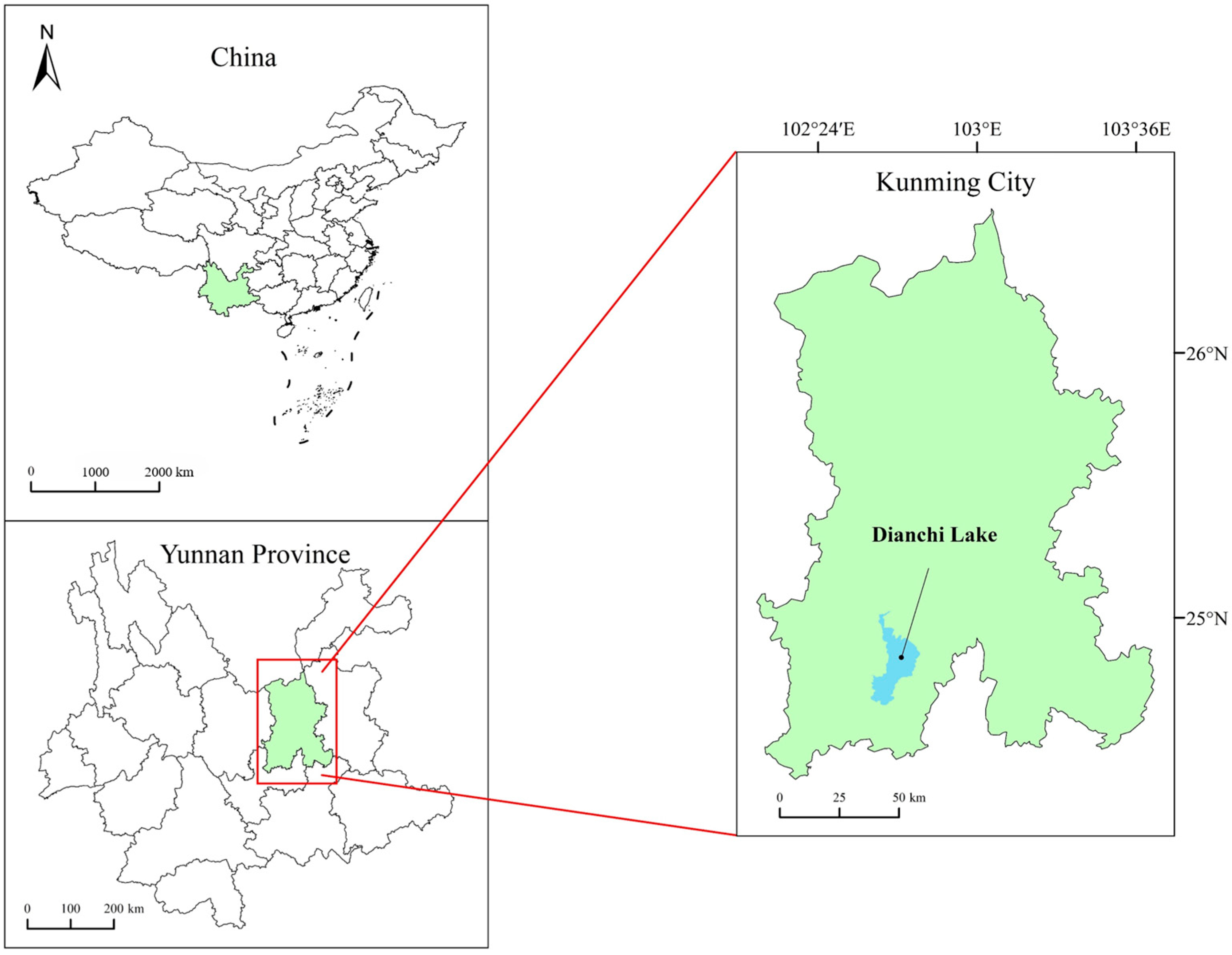
2.1. Study Area
2.2. Data Processing
2.3. Analytical Method
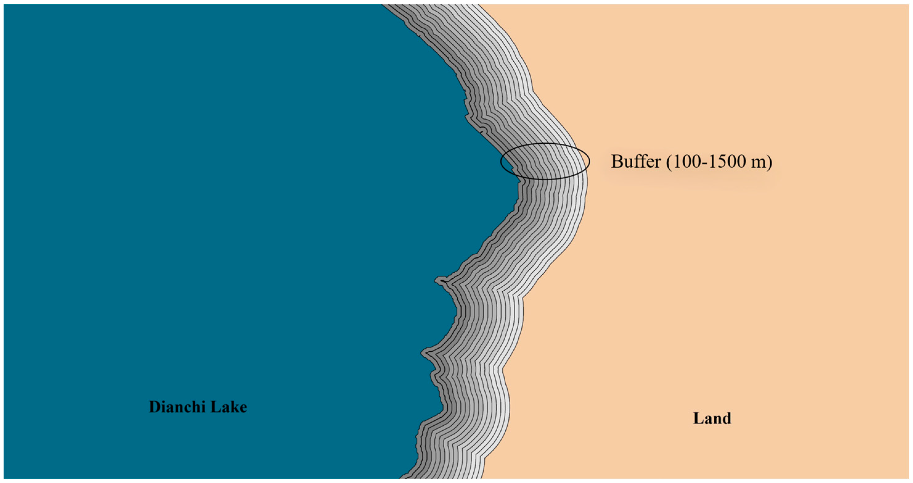
2.3.1. Buffer Establishment and Cooling Effect Quantification
2.3.2. Partition of LST According to LCLU
2.3.3. Multi-Level Differential Analysis of the Cooling Effect
3. Results and Discussion
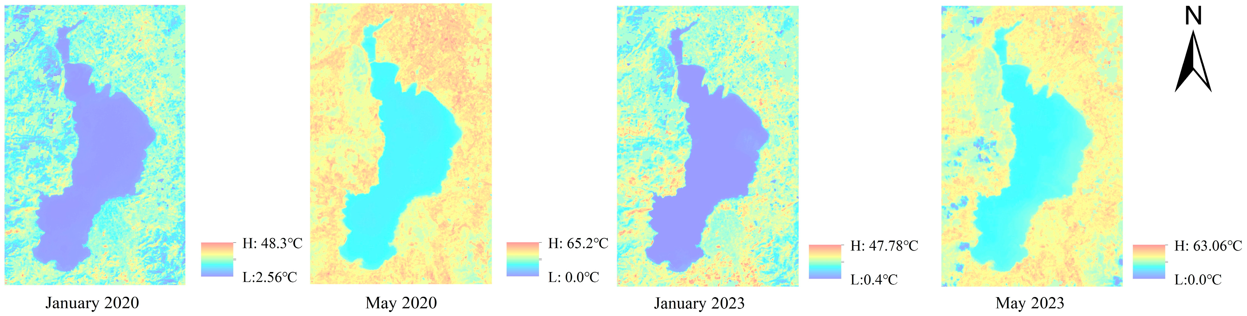
3.1. Spatial Distribution Variation
3.2. Seasonal Differences in Cooling Effects
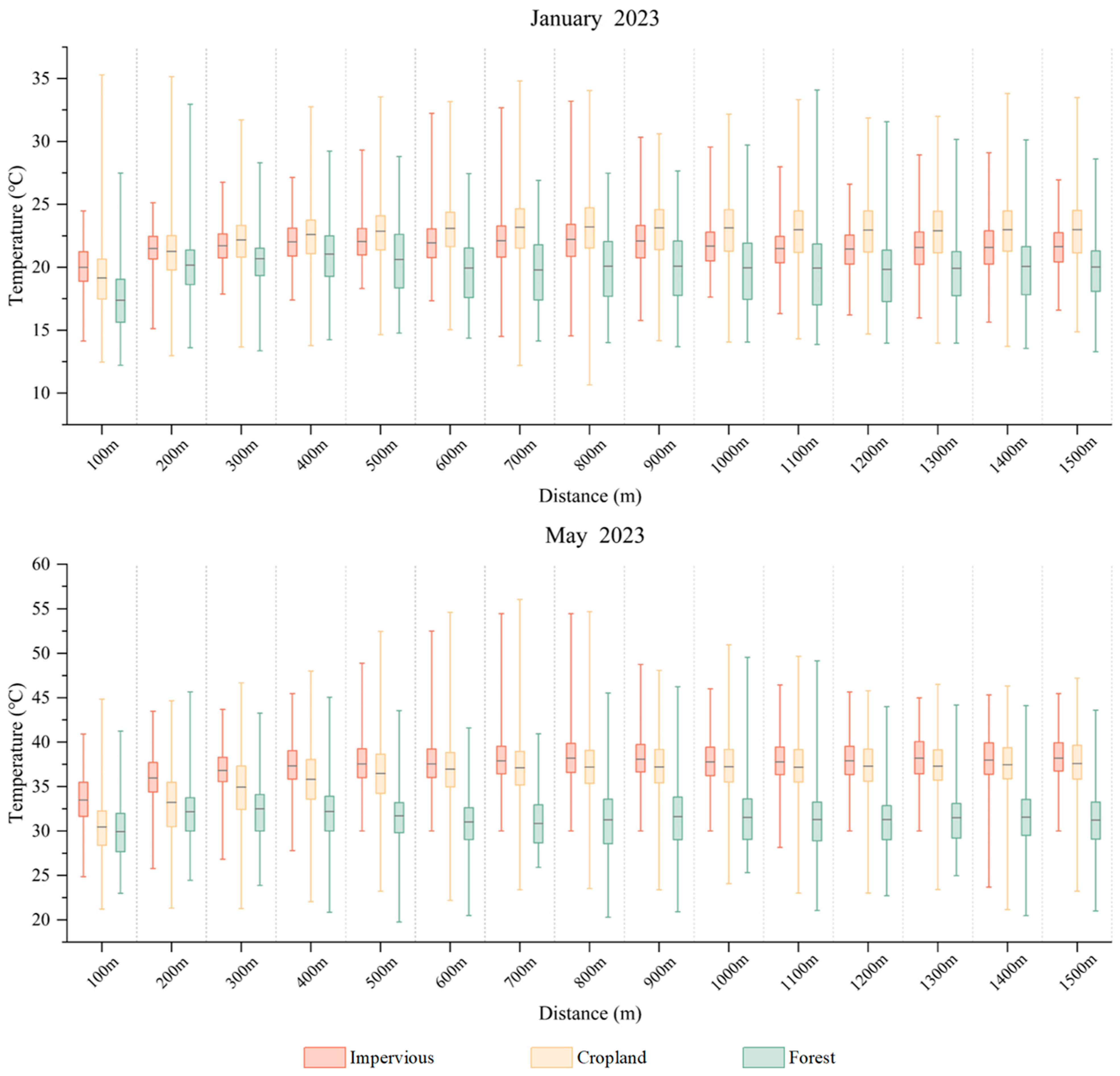
3.3. Sensitivities of Different Surfaces to Cooling Effects
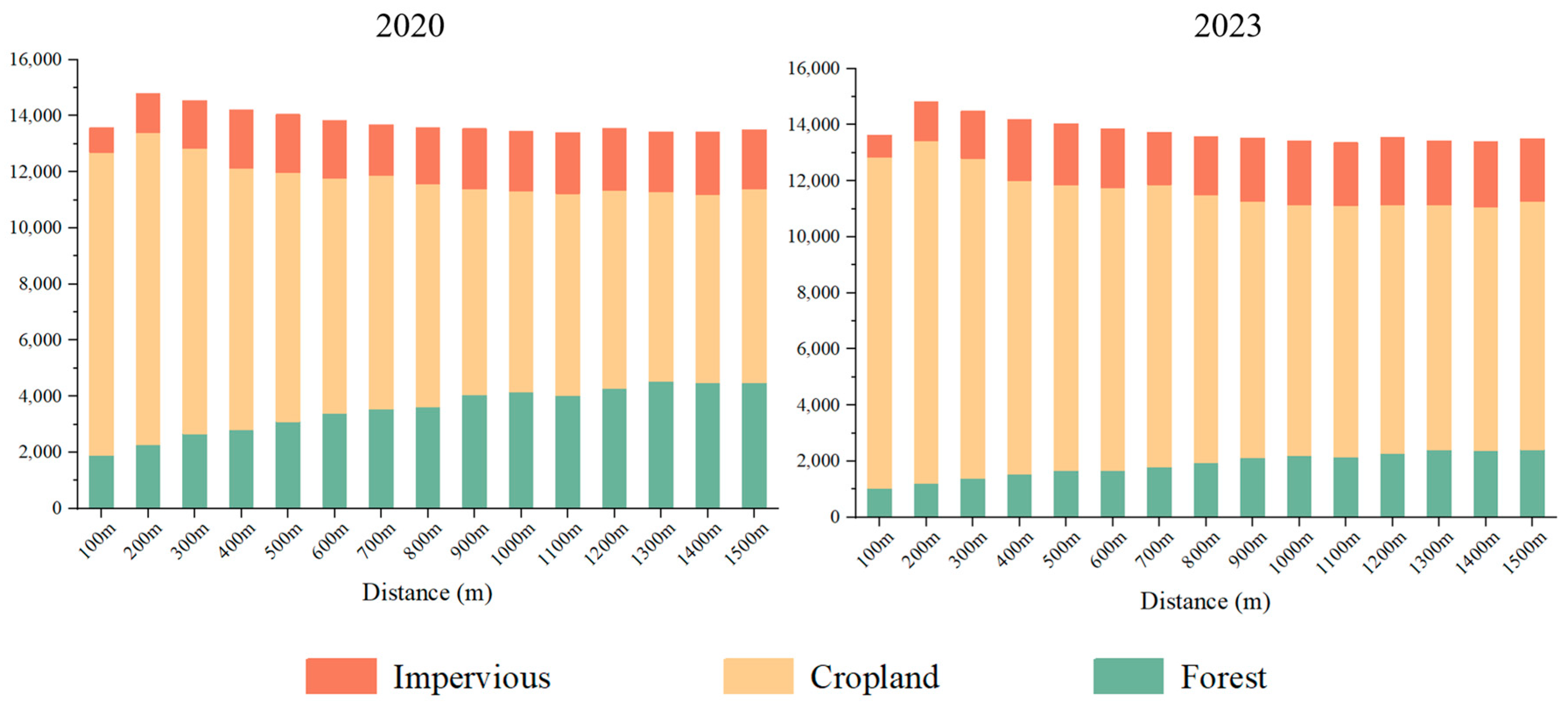
3.3.1. Variations in LCD and LCI
- (1)
- The effective range of water body cooling is closely tied to underlying surface characteristics, with land cover types significantly modulating the spatial extent of cooling effects.
- (2)
- The cooling capacity of the same water body displays selective responses to different land cover types, exhibiting pronounced spatial limitations in temperature regulation for artificial impervious surfaces.
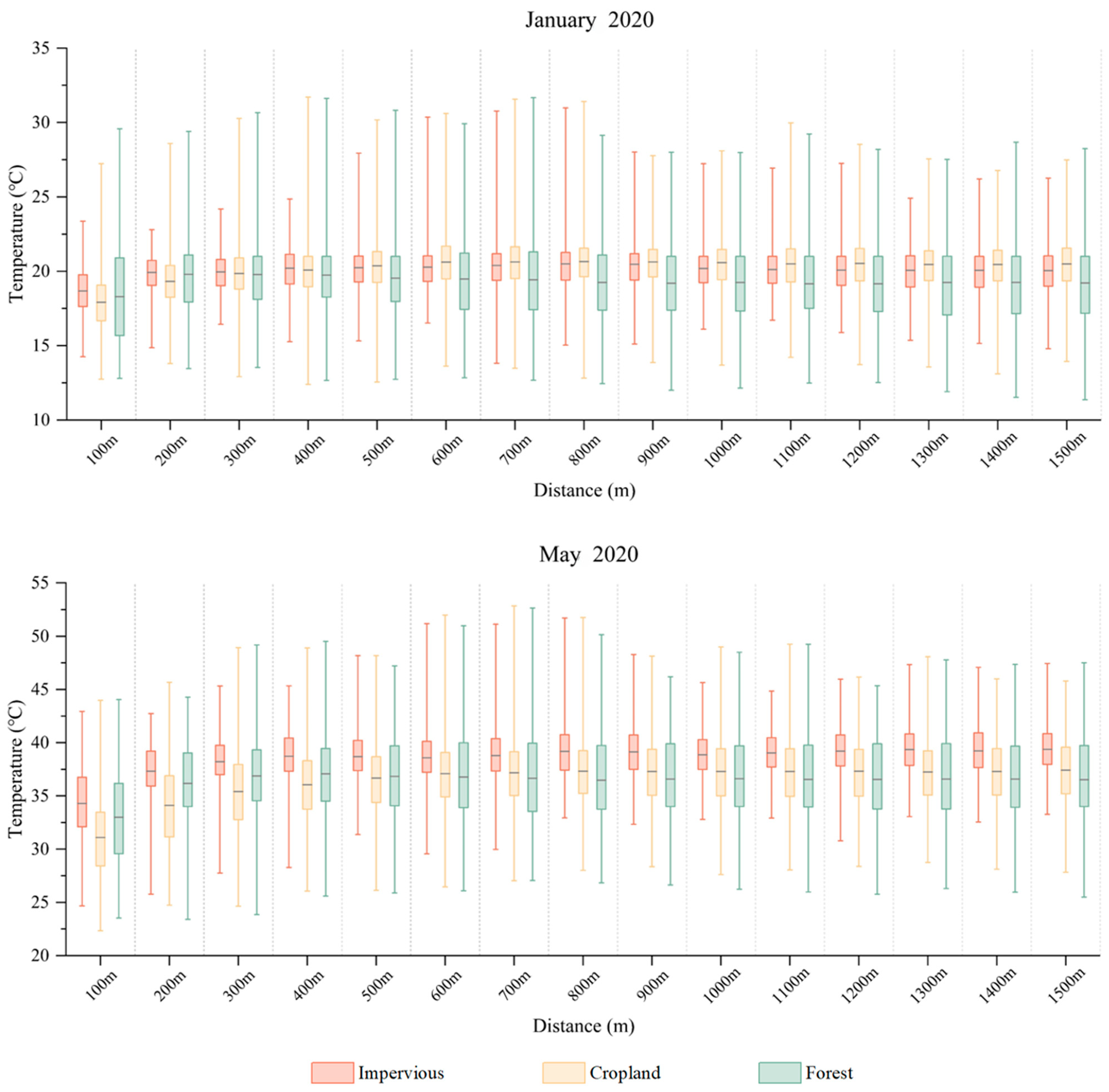
3.3.2. Thermal Distribution Differences
4. Conclusions
- (1)
- The surface temperature distribution along the Dianchi Lake shoreline exhibits a correlation with the land use type. High-temperature zones are predominantly clustered in the urban core areas of the eastern shoreline, whereas low-temperature zones are primarily concentrated in the forested regions of the western shoreline. Spatially heterogeneous land cover distributions across the eastern and western shores of Dianchi Lake contribute to thermal environmental disparities.
- (2)
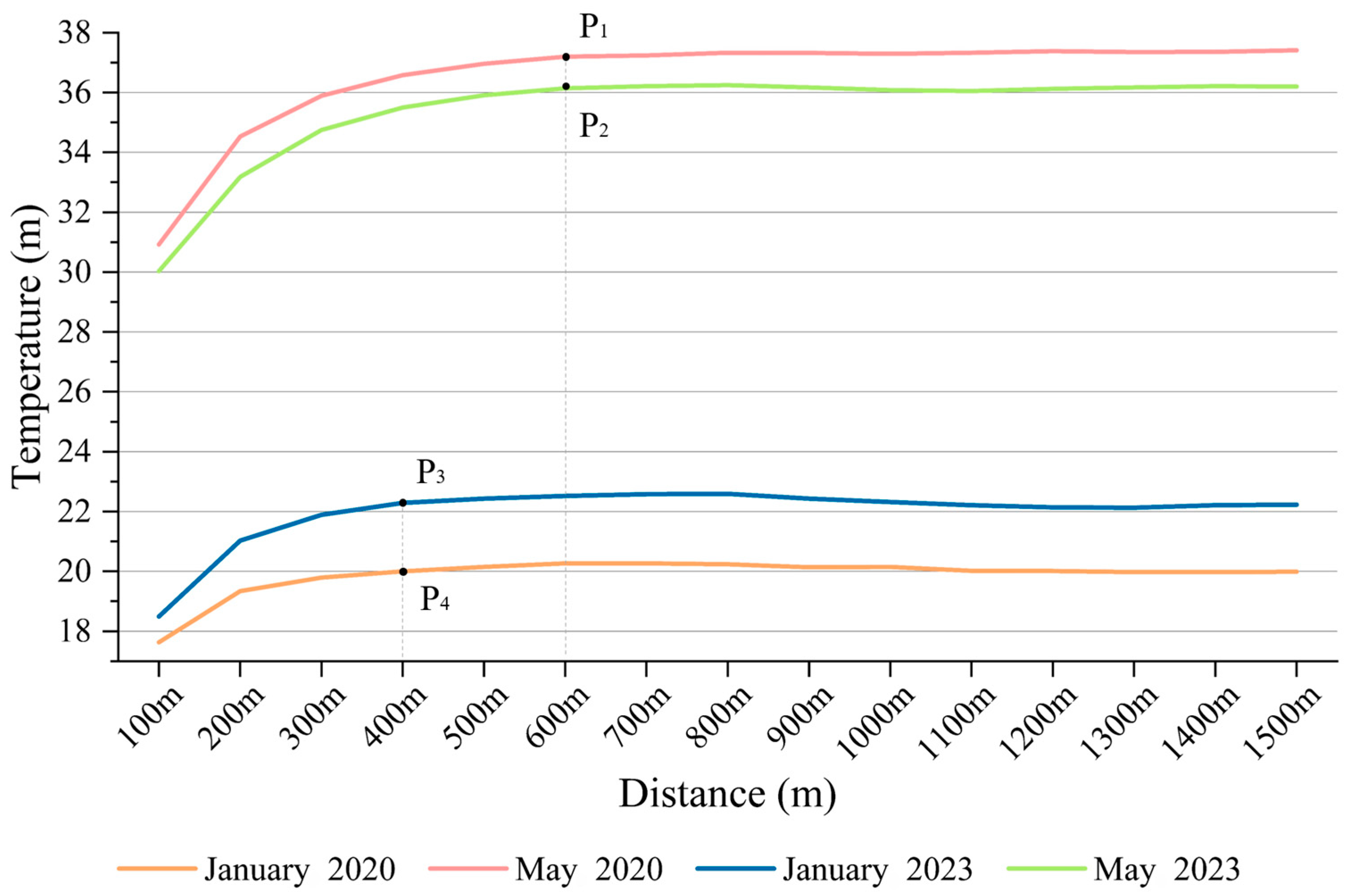
- The LCD exhibits a spatial extent of approximately 400 m, with LCI ranging from 2.4 to 3.9 °C during dry seasons, whereas in rainy seasons, it demonstrates an expanded LCD of 600 m and enhanced LCI between 6.0 and 6.6 °C. From the perspective of seasonal variation, both the effective radius and thermal mitigation magnitude of the cooling effect surpass those observed in dry seasons during the rainy period.
- (3)
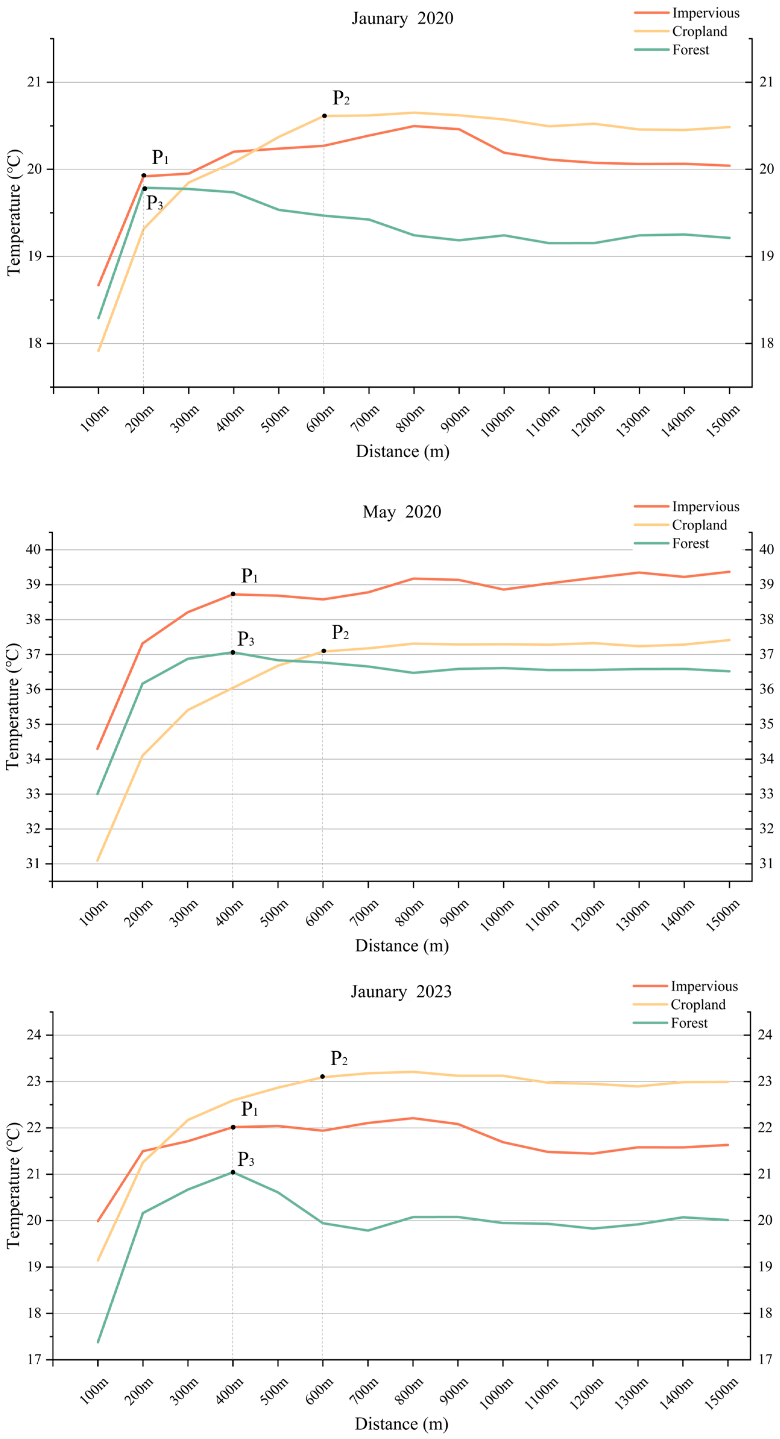
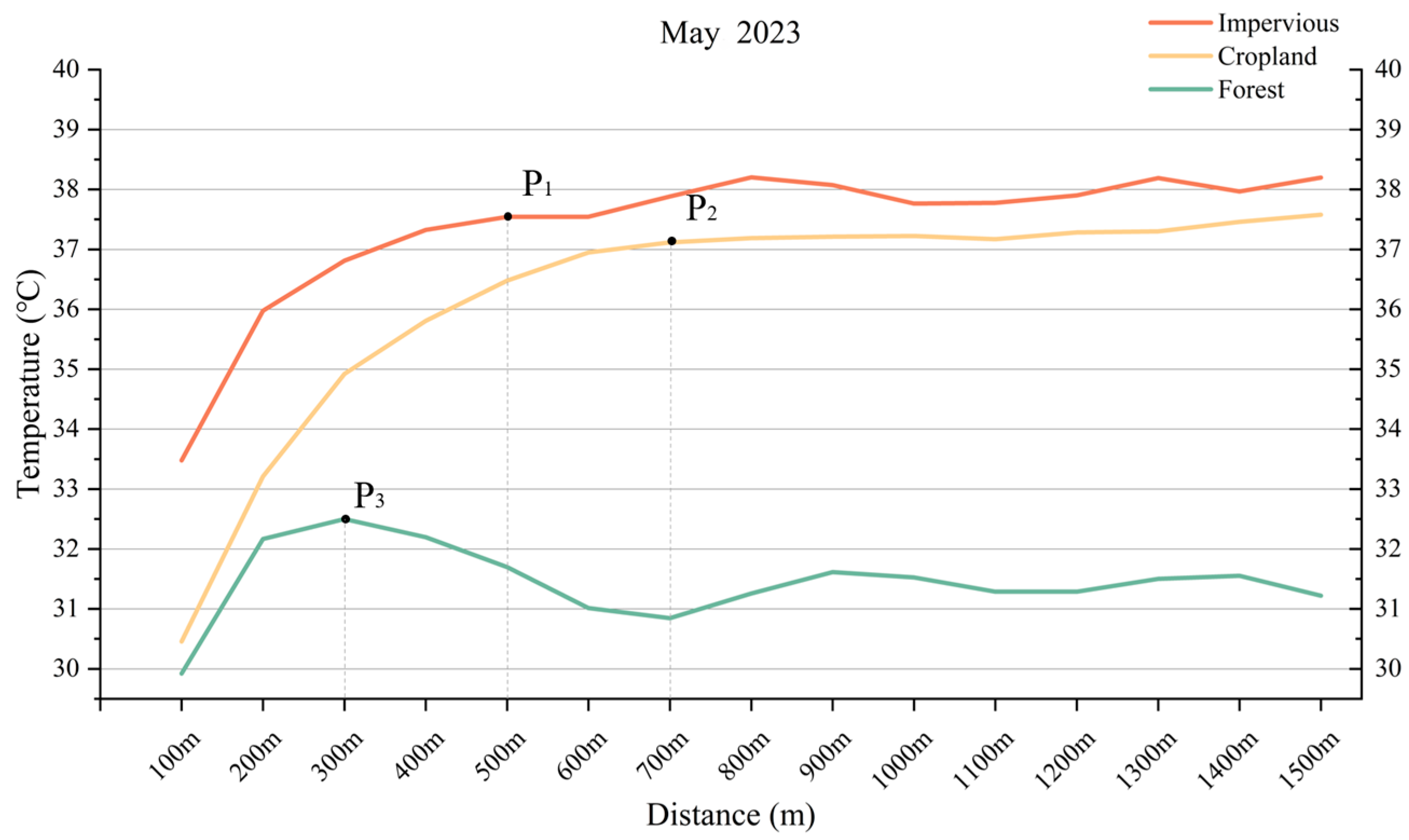
- Dianchi Lake manifests differential cooling ranges across distinct land use types. The cooling effect demonstrates the most extensive LCD range on agricultural lands, reaching 600 m, which is followed by 400 m for impervious surfaces. In contrast, forested areas exhibit LCD only within a 100-m radius. Impervious surfaces display the highest sensitivity to cooling effects, followed by agricultural lands, whereas forested areas exhibit the lowest responsiveness among the three surface types.
Author Contributions
Funding
Institutional Review Board Statement
Informed Consent Statement
Data Availability Statement
Conflicts of Interest
Abbreviations
| UHI | Urban heat island |
| LST | Land surface temperature |
| LCLU | Land cover and land use |
| LCI | Lake cooling intensity |
| LCD | Lake cooling distance |
References
- Yuan, C.; Zhu, R.; Tong, S.; Mei, S.; Zhu, W. Impact of Anthropogenic Heat from Air-Conditioning on Air Temperature of Naturally Ventilated Apartments at High-Density Tropical Cities. Energy Build. 2022, 268, 112171. [Google Scholar]
- Zhou, L.; Hu, F.; Wang, B.; Wei, C.; Sun, D.; Wang, S. Relationship between Urban Landscape Structure and Land Surface Temperature: Spatial Hierarchy and Interaction Effects. Sustain. Cities Soc. 2022, 80, 103795. [Google Scholar]
- Oke, T.R. City size and the urban heat island. Atmos. Environ. 1967 1973, 7, 769–779. [Google Scholar]
- Patz, J.A.; Campbell-Lendrum, D.; Holloway, T.; Foley, J.A. Impact of regional climate change on human health. Nature 2005, 438, 310–317. [Google Scholar]
- Ca, V.T.; Asaeda, T.; Abu, E.M. Reductions in air conditioning energy caused by a nearby park. Energy Build. 1998, 29, 83–92. [Google Scholar]
- Grimm, N.B.; Faeth, S.H.; Golubiewski, N.E.; Redman, C.L.; Wu, J.; Bai, X.; Briggs, J.M. Global Change and the Ecology of Cities. Science 2008, 319, 756. [Google Scholar]
- Kalisa, E.; Fadlallah, S.; Amani, M.; Nahayo, L.; Habiyaremye, G. Temperature and air pollution relationship during heatwaves in Birmingham, UK. Sustain. Cities Soc. 2018, 43, 111–120. [Google Scholar]
- Lo, C.P.; Quattrochi, D.A. Land-Use and Land-Cover Change, Urban Heat Island Phenomenon, and Health Implications: A Remote Sensing Approach. Photogramm. Eng. Remote Sens. 2003, 69, 1053–1063. [Google Scholar]
- Wang, Y.; Du, H.; Xu, Y.; Lu, D.; Wang, X.; Guo, Z. Temporal and spatial variation relationship and influence factors on surface urban heat island and ozone pollution in the Yangtze River Delta, China. Sci. Total Environ. 2018, 631, 921–933. [Google Scholar]
- Bartesaghi Koc, C.; Osmond, P.; Peters, A. Evaluating the cooling effects of green infrastructure: A systematic review of methods, indicators and data sources. Sol. Energy 2018, 166, 486–508. [Google Scholar]
- Bowler, D.E.; Buyung-Ali, L.; Knight, T.M.; Pullin, A.S. Urban greening to cool towns and cities: A systematic review of the empirical evidence. Landsc. Urban Plan. 2010, 97, 147–155. [Google Scholar]
- Deilami, K.; Kamruzzaman, M.; Liu, Y. Urban heat island effect: A systematic review of spatio-temporal factors, data, methods, and mitigation measures. Int. J. Appl. Earth Obs. Geoinf. 2018, 67, 30–42. [Google Scholar]
- Lamb, W.F.; Creutzig, F.; Callaghan, M.W.; Minx, J.C. Learning about urban climate solutions from case studies. Nat. Clim. Change 2019, 9, 279. [Google Scholar]
- Gunawardena, K.R.; Wells, M.J.; Kershaw, T. Utilising green and bluespace to mitigate urban heat island intensity. Sci. Total Environ. 2017, 584, 1040–1055. [Google Scholar]
- Cheng, L.; Guan, D.; Zhou, L.; Zhao, Z.; Zhou, J. Urban cooling island effect of main river on a landscape scale in Chongqing. China. Sustain. Cities Soc. 2019, 47, 101501. [Google Scholar]
- Du, H.; Song, X.; Jiang, H.; Kan, Z.; Wang, Z.; Cai, Y. Research on the cooling island effects of water body: A case study of Shanghai, China. Ecol. Indic. 2016, 67, 31–38. [Google Scholar]
- Chang, C.; Li, M.; Chang, S. A preliminary study on the local cool-island intensity of Taipei city parks. Landsc. Urban Plan. 2007, 80, 386–395. [Google Scholar]
- Hathway, E.A.; Sharples, S. The interaction of rivers and urban form in mitigating the Urban Heat Island effect: A UK case study. Build. Environ. 2012, 58, 14–22. [Google Scholar]
- Moyer, A.N.; Hawkins, T.W. River effects on the heat island of a small urban area. Urban Clim. 2017, 21, 262–277. [Google Scholar]
- Murakawa, S.; Sekine, T.; Narita, K.I.; Nishina, D. Study of the effects of a river on the thermal environment in an urban area. Energy Build. 1991, 16, 993–1001. [Google Scholar]
- Jiang, L.; Liu, S.; Liu, C.; Feng, Y. How do urban spatial patterns influence the river cooling effect? A case study of the Huangpu Riverfront in Shanghai, China. Sustain. Cities Soc. 2021, 69, 102835. [Google Scholar]
- Xue, Z.; Hou, G.; Zhang, Z.; Lyu, X.; Jiang, M.; Zou, Y.; Shen, X.; Wang, J.; Liu, X. Quantifying the cooling-effects of urban and peri-urban wetlands using remote sensing data: Case study of cities of Northeast China. Landsc. Urban Plan. 2019, 182, 92–100. [Google Scholar]
- Sun, R.; Chen, L. How can urban water bodies be designed for climate adaptation? Landsc. Urban Plan. 2012, 105, 27–33. [Google Scholar]
- Wu, J.; Li, C.; Zhang, X.; Zhao, Y.; Liang, J.; Wang, Z. Seasonal variations and main influencing factors of the water cooling islands effect in Shenzhen. Ecol. Indic. 2020, 117, 106699. [Google Scholar]
- Verhagen, W.; Van Teeffelen, A.J.A.; Compagnucci, A.B.; Poggio, L.; Gimona, A.; Verburg, P.H. Effects of landscape configuration on mapping ecosystem service capacity: A review of evidence and a case study in Scotland. Landsc. Ecol. 2016, 31, 1457–1479. [Google Scholar]
- Sun, R.; Chen, L. Effects of green space dynamics on urban heat islands: Mitigation and diversification. Ecosyst. Serv. 2017, 23, 38–46. [Google Scholar]
- Peng, J.; Liu, Q.; Xu, Z.; Lyu, D.; Du, Y.; Qiao, R.; Wu, J. How to effectively mitigate urban heat island effect? A perspective of waterbody patch size threshold. Landsc. Urban Plan. 2020, 202, 103873. [Google Scholar]
- Jiang, Y.; Huang, J.; Shi, T.; Li, X. Cooling Island Effect of Blue-Green Corridors: Quantitative Comparison of Morphological Impacts. Int. J. Environ. Res. Public Health 2021, 18, 11917. [Google Scholar]
- Kang, X.M.; Cui, L.J.; Zhao, X.S. Analysis on the function of relieving heat island effect in wetland in Beijing. Chin. Agric. Sci. Bull. 2015, 31, 199–205. [Google Scholar]
- Wang, Y.; Ouyang, W. Investigating the heterogeneity of water cooling effect for cooler cities. Sustain. Cities Soc. 2021, 75, 103281. [Google Scholar]
- Peng, J.; Dan, Y.; Qiao, R.; Liu, Y.; Dong, J.; Wu, J. How to quantify the cooling effect of urban parks? Linking maximum and accumulation perspectives. Remote Sens. Environ. 2021, 252, 112135. [Google Scholar]
- Toparlar, Y.; Blocken, B.; Maiheu, B.; van Heijst, G.J.F. The effect of an urban park on the microclimate in its vicinity: A case study for Antwerp, Belgium. Int. J. Climatol. 2018, 38, E303–E322. [Google Scholar]
- Cheng, X.; Wei, B.; Chen, G.; Li, J.; Song, C. Influence of park size and its surrounding urban landscape patterns on the park cooling effect. J. Urban Plan. Dev. 2015, 141, A4014002. [Google Scholar]
- Zhou, Y.; Gao, W.; Yang, C.; Shen, Y. Exploratory analysis of the influence of landscape patterns on lake cooling effect in Wuhan, China. Urban Clim. 2021, 39, 100969. [Google Scholar]
- Feyisa, G.L.; Dons, K.; Meilby, H. Efficiency of parks in mitigating urban heat island effect: An example from Addis Ababa. Landsc. Urban Plan. 2014, 123, 87–95. [Google Scholar]
- Yang, K.; Yu, Z.; Luo, Y.; Yang, Y.; Zhao, L.; Zhou, X. Spatial and temporal variations in the relationship between lake water surface temperatures and water quality—A case study of Dianchi Lake. Sci. Total Environ. 2018, 624, 859–871. [Google Scholar]
- Zhan, X.; Bo, Y.; Zhou, F.; Liu, X.; Paerl, H.W.; Shen, J.; Wang, R.; Li, F.; Tao, S.; Dong, Y.; et al. Evidence for the Importance of Atmospheric Nitrogen Deposition to Eutrophic Lake Dianchi, China. Environ. Sci. Technol. 2017, 51, 6699–6708. [Google Scholar]
- Gómez, C.; White, J.C.; Wulder, M.A. Optical remotely sensed time series data for land cover classification: A review. ISPRS J. Photogramm. Remote Sens. 2016, 116, 55–72. [Google Scholar]
- Calderón-Loor, M.; Hadjikakou, M.; Bryan, B.A. High-resolution wall-to-wall land-cover mapping and land change assessment for Australia from 1985 to 2015. Remote Sens. Environ. 2021, 252, 112148. [Google Scholar]
- Yang, J.; Huang, X. The 30 m annual land cover dataset and its dynamics in China from 1990 to 2019. Earth Syst. Sci. Data 2021, 13, 3907–3925. [Google Scholar]
- Wu, C.; Lung, S.C.; Jan, J. Development of a 3-D urbanization index using digital terrain models for surface urban heat island effects. ISPRS J. Photogramm. Remote Sens. 2013, 81, 1–11. [Google Scholar]
- Zhou, X.; Chen, H. Impact of urbanization-related land use land cover changes and urban morphology changes on the urban heat island phenomenon. Sci. Total Environ. 2018, 635, 1467–1476. [Google Scholar] [PubMed]
- Smith, W.K.; Nobel, P.S. Influences of seasonal changes in leaf morphology on water-use efficiency for three desert broadleaf shrubs. Ecology 1977, 58, 1033–1043. [Google Scholar]


| Data | Source | Resolution |
|---|---|---|
| LST | USGA (http://earthexplorer.usgs.gov) | 30 m |
| Lake shape | Open Street Map (https://openstreetmap.us) | 10 m |
| Land cover | Zendo (https://zenodo.org/records/12779975) | 30 m |
| Metrics | Description | Acquisition Methods |
|---|---|---|
| LST | Land surface temperature; different land use types correspond to distinct surface temperatures | Satellite remote sensing images |
| Buffer | A distance interval established based on lakeshore representing the same influence by the lake | Established in ArcMap based on the Dianchi lakeshore |
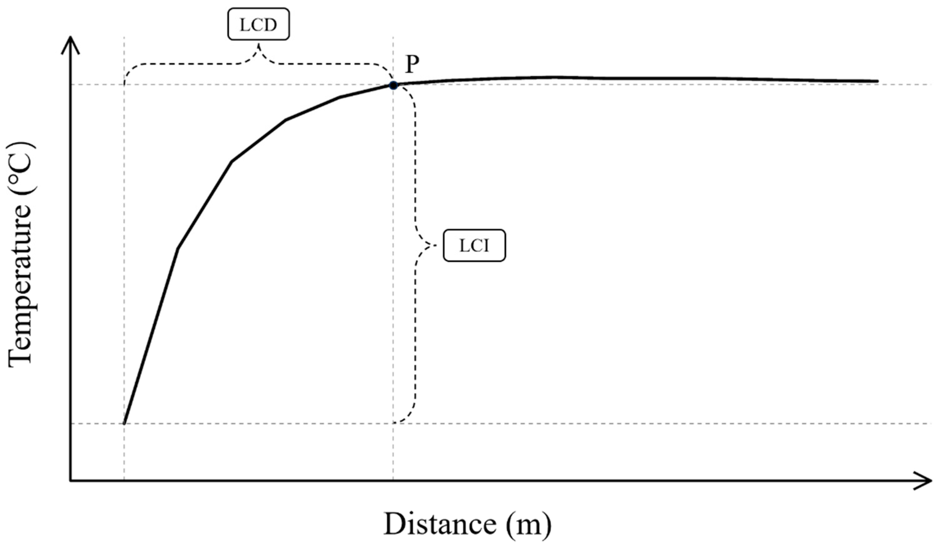
| Point P | The first inflection point with a temperature variation of less than 0.1 °C | Data analysis |
| LCD | The distance corresponding to point P | Data analysis |
| LCI | The temperature difference between the cooling boundary and the water shoreline | Data analysis |
Disclaimer/Publisher’s Note: The statements, opinions and data contained in all publications are solely those of the individual author(s) and contributor(s) and not of MDPI and/or the editor(s). MDPI and/or the editor(s) disclaim responsibility for any injury to people or property resulting from any ideas, methods, instructions or products referred to in the content. |
© 2025 by the authors. Licensee MDPI, Basel, Switzerland. This article is an open access article distributed under the terms and conditions of the Creative Commons Attribution (CC BY) license (https://creativecommons.org/licenses/by/4.0/).
Share and Cite
Wang, Z.; Ma, Z.; Chen, Y.; Zhu, P.; Wang, L. Assessing the Cooling Effects of Water Bodies Based on Urban Environments: Case Study of Dianchi Lake in Kunming, China. Atmosphere 2025, 16, 856. https://doi.org/10.3390/atmos16070856
Wang Z, Ma Z, Chen Y, Zhu P, Wang L. Assessing the Cooling Effects of Water Bodies Based on Urban Environments: Case Study of Dianchi Lake in Kunming, China. Atmosphere. 2025; 16(7):856. https://doi.org/10.3390/atmos16070856
Chicago/Turabian StyleWang, Zhihao, Ziyang Ma, Yifei Chen, Pengkun Zhu, and Lu Wang. 2025. "Assessing the Cooling Effects of Water Bodies Based on Urban Environments: Case Study of Dianchi Lake in Kunming, China" Atmosphere 16, no. 7: 856. https://doi.org/10.3390/atmos16070856
APA StyleWang, Z., Ma, Z., Chen, Y., Zhu, P., & Wang, L. (2025). Assessing the Cooling Effects of Water Bodies Based on Urban Environments: Case Study of Dianchi Lake in Kunming, China. Atmosphere, 16(7), 856. https://doi.org/10.3390/atmos16070856