

Simulating Lightning Discharges: The Influence of Environmental Conditions on Ionization and Spark Behavior

Abstract
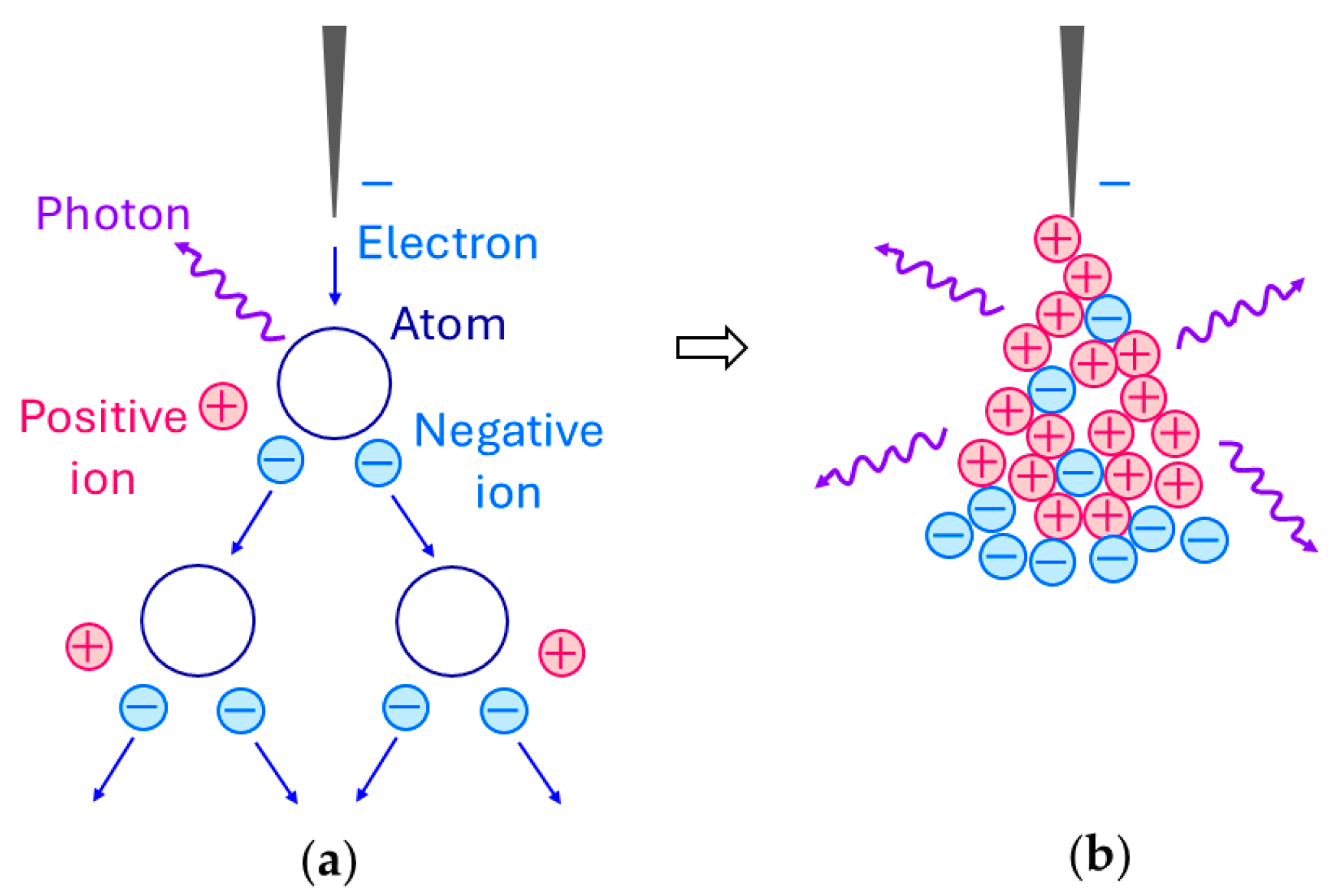
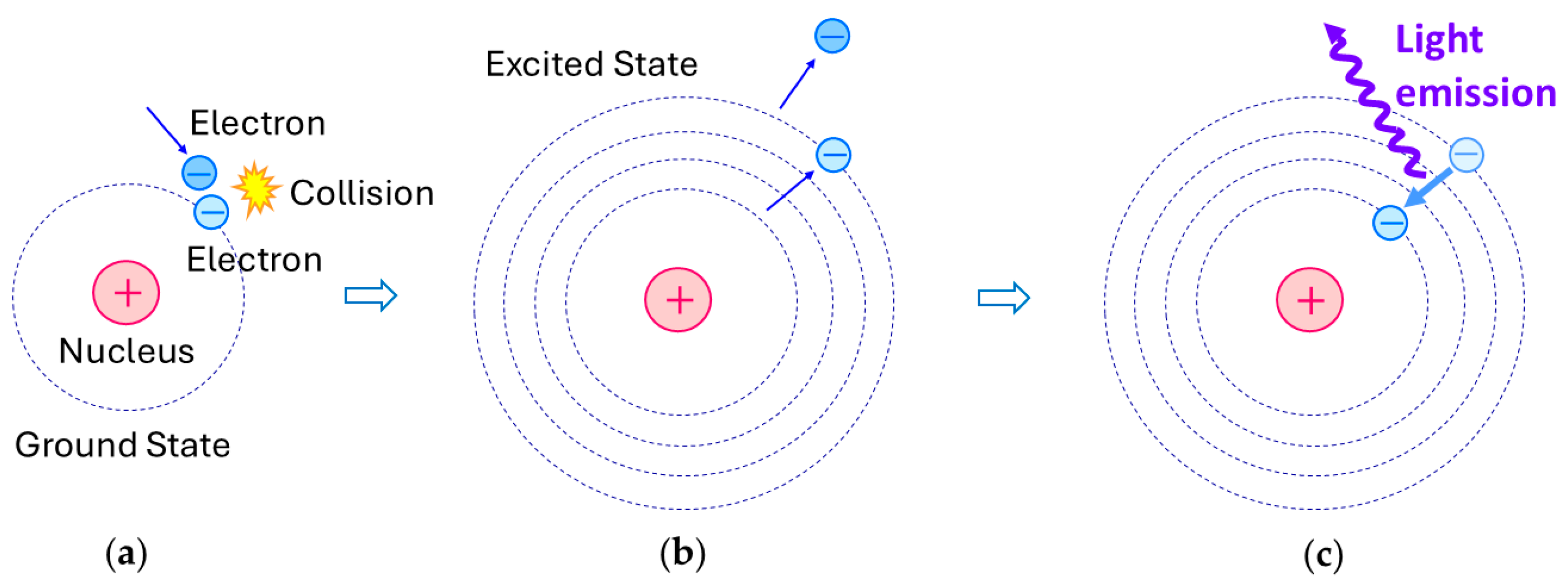
1. Introduction
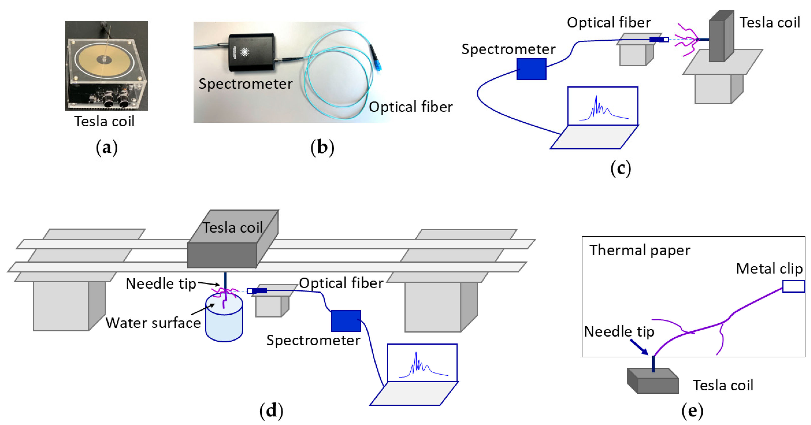
2. Materials and Methods
3. Results
3.1. Spectral Analysis
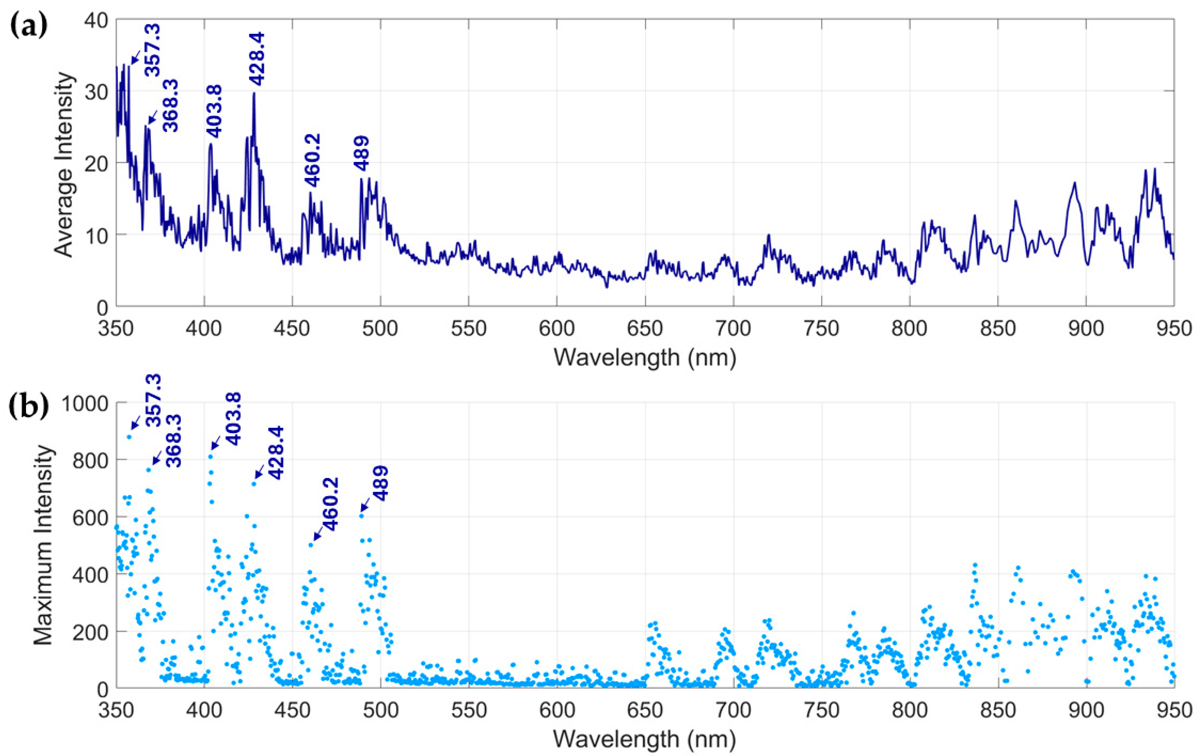
3.1.1. Spectrum of Discharge in Air
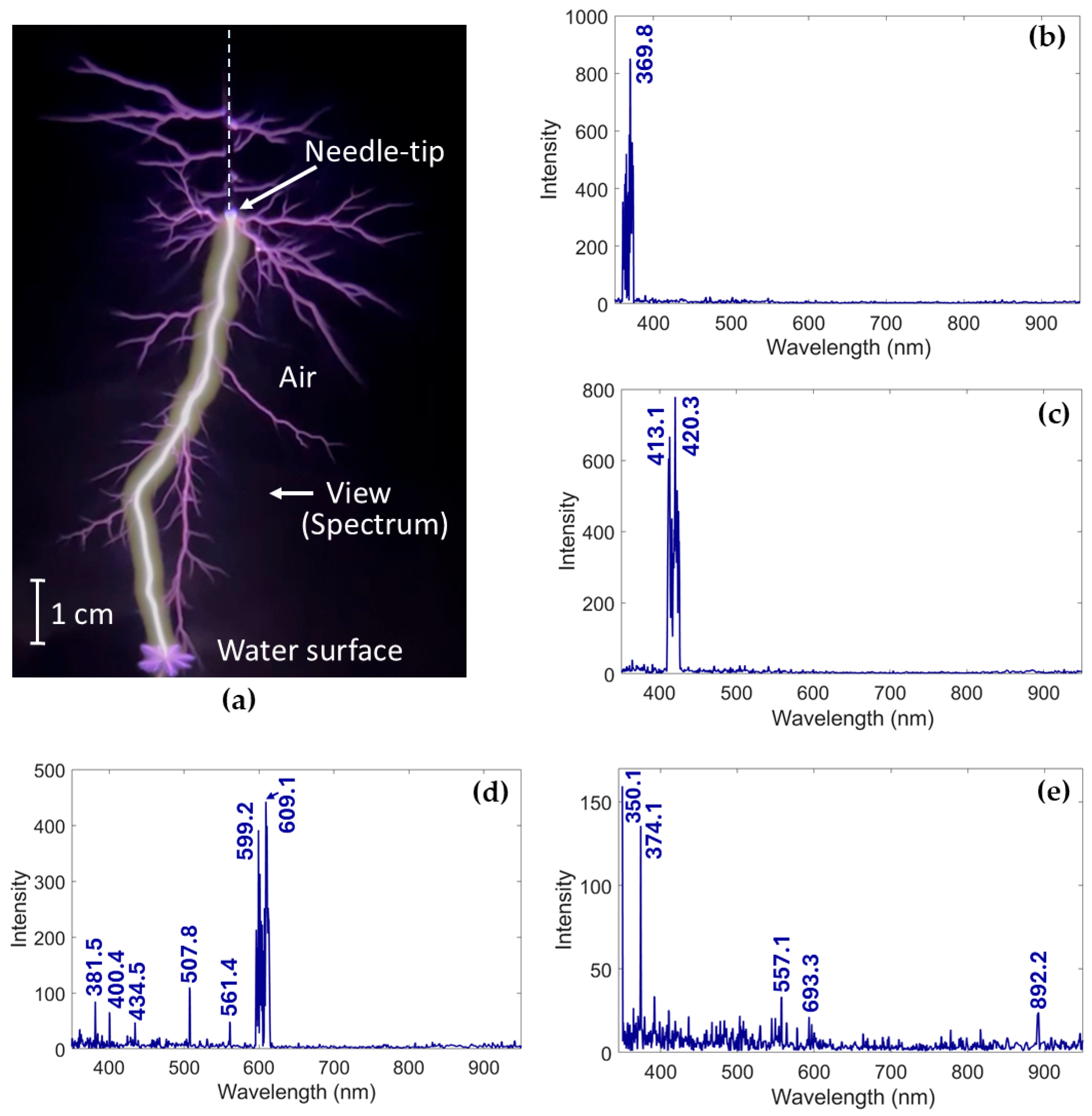
3.1.2. Spectrum of Discharge Toward Water Surface
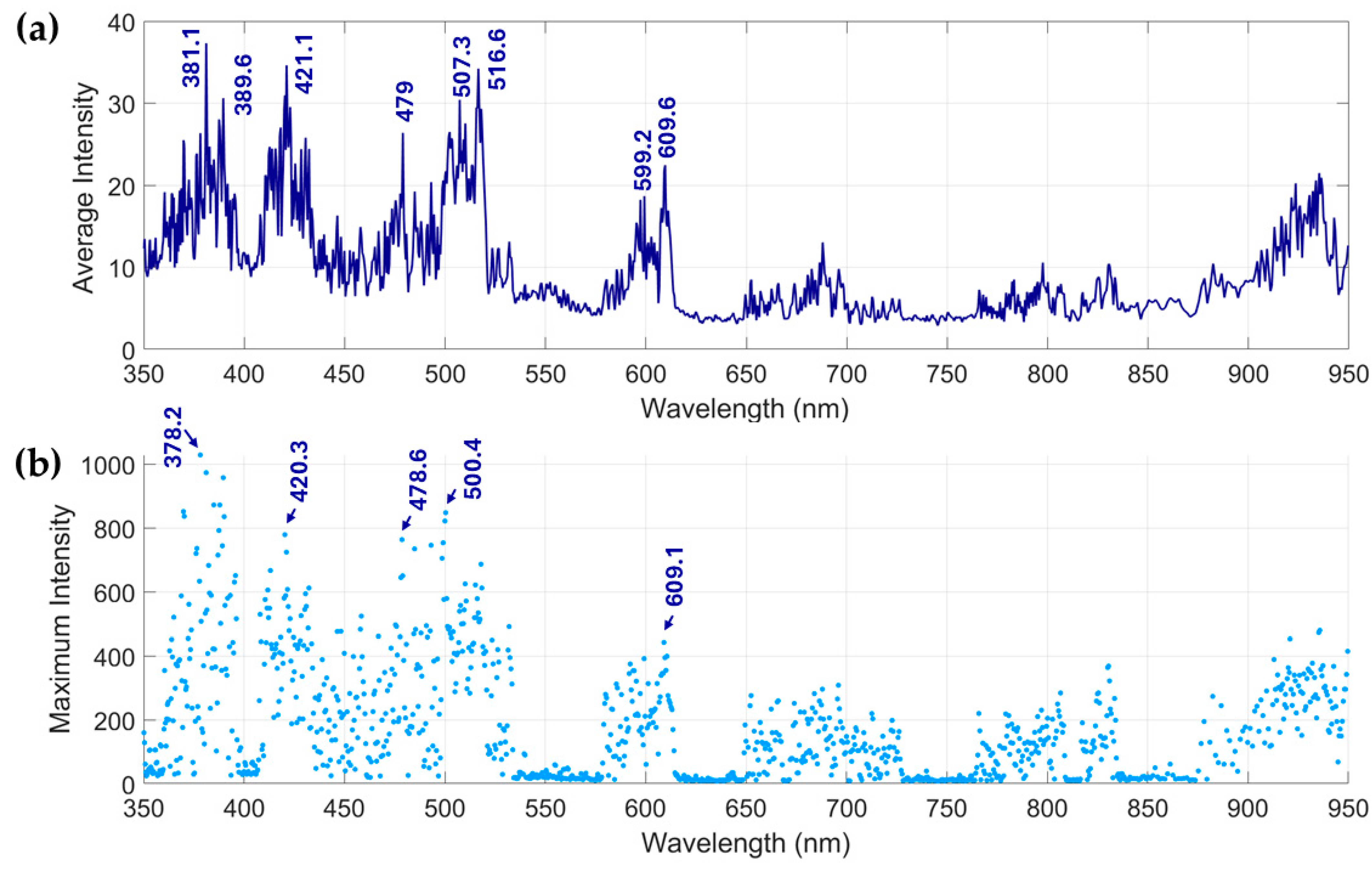
3.1.3. Comparison Between the Spectrum of Tesla Coil Discharges and Lightning Emissions
3.2. Spark Discharge in Various Air Conditions
3.2.1. Spark Discharge in Air Versus Moist Air
3.2.2. Discharge Path Length in Various Air Conditions
3.2.3. Electric Field Measurements of Discharge in Air Versus Moist Air
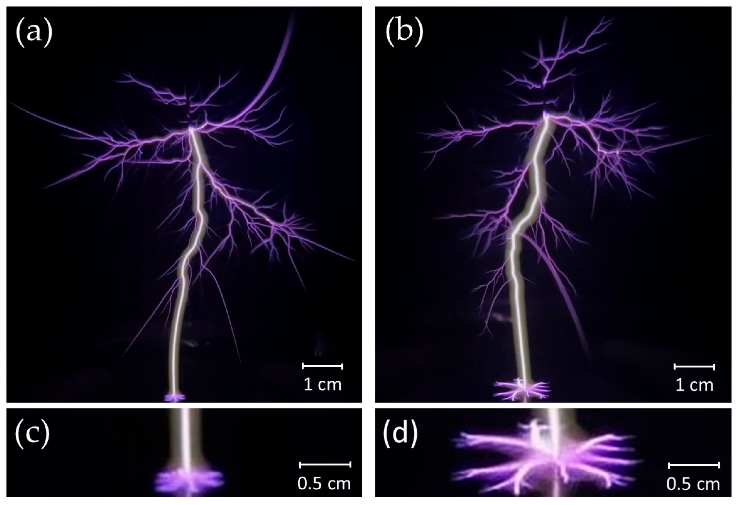
3.3. Discharge over Various Water Surfaces
3.3.1. Star-Shaped Discharge over Tap Water Versus DI Water
3.3.2. Star-Shaped Discharge over DI Water with NaCl
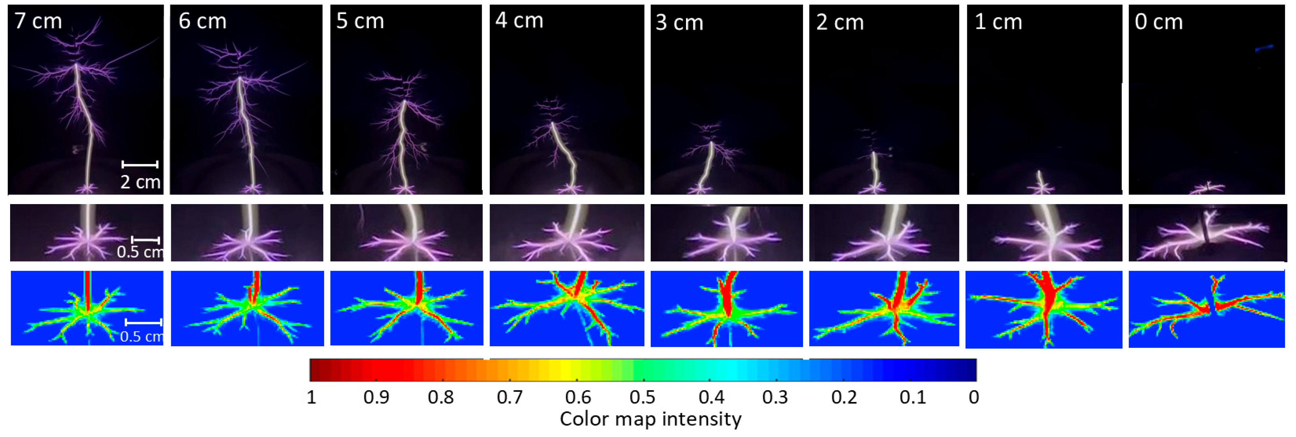
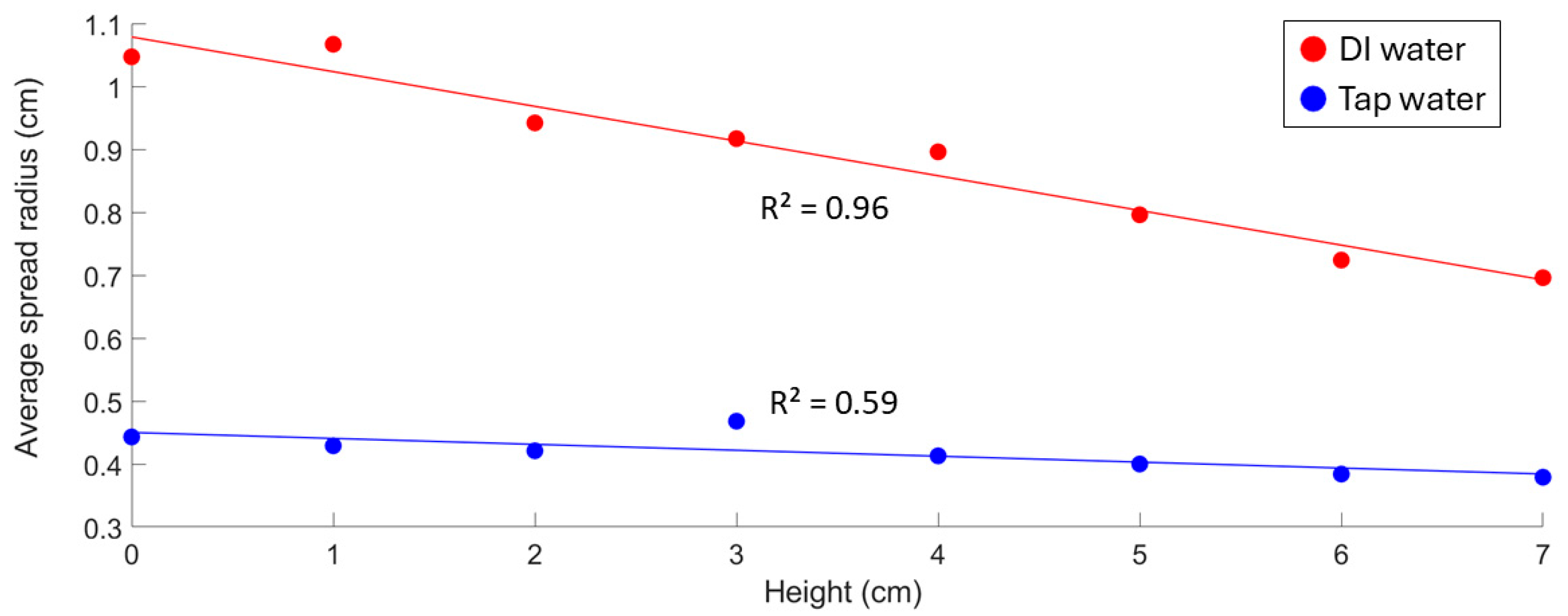
3.3.3. Spark Discharge Height Versus Star-Shaped Discharge Path Length
4. Discussion
5. Conclusions
Supplementary Materials
Author Contributions
Funding
Institutional Review Board Statement
Informed Consent Statement
Data Availability Statement
Acknowledgments
Conflicts of Interest
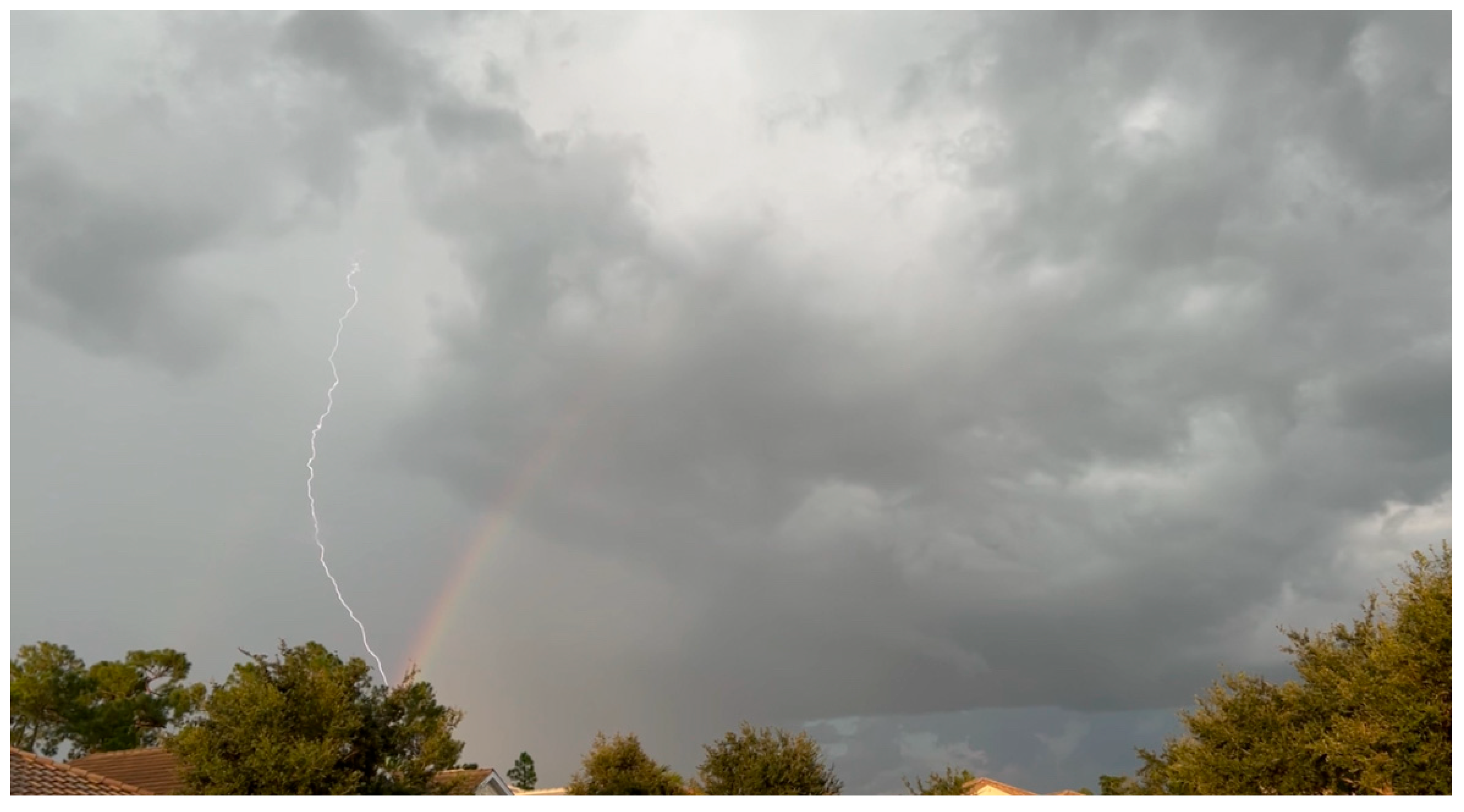
Appendix A. Lightning and Rainbow Coexistence in the Atmosphere
References
- Rakov, V.A.; Uman, M.A. Lightning: Physics and Effects; Cambridge University Press: Cambridge, UK, 2003. [Google Scholar]
- Green, G.; Watanabe, N. Green Flashes Observed in Optical and Infrared during an Extreme Electric Storm. Appl. Sci. 2024, 14, 6938. [Google Scholar]
- Peterson, M.; Lay, E. GLM observations of the brightest lightning in the Americas. J. Geophys. Res. Atmos. 2020, 125, e2020JD033378. [Google Scholar]
- Asfur, M.; Price, C.; Silverman, J.; Wishkerman, A. Why is lightning more intense over the oceans? J. Atmos. Sol.-Terr. Phys. 2020, 202, 105259. [Google Scholar]
- Christian, H.J.; Blakeslee, R.J.; Boccippio, D.J.; Boeck, W.L.; Buechler, D.E.; Driscoll, K.T.; Goodman, S.J.; Hall, J.M.; Koshak, W.J.; Mach, D.M.; et al. Global frequency and distribution of lightning as observed from space by the Optical Transient Detector. J. Geophys. Res. Atmos. 2003, 108, ACL-4. [Google Scholar]
- van der Velde, O.A.; Montanyà, J. Statistics and variability of the altitude of elves. Geophys. Res. Lett. 2016, 43, 5467–5474. [Google Scholar]
- Lyons, W.A.; Uliasz, M.; Nelson, T.E. Large peak current cloud-to-ground lightning flashes during the summer months in the contiguous United States. Mon. Weather Rev. 1998, 126, 2217–2233. [Google Scholar]
- Dwyer, J.R.; Uman, M.A. The physics of lightning. Phys. Rep. 2014, 534, 147–241. [Google Scholar]
- Nijdam, S.; Teunissen, J.; Ebert, U. The physics of streamer discharge phenomena. Plasma Sources Sci. Technol. 2020, 29, 103001. [Google Scholar]
- Xie, S.; Zeng, R.; Li, J.; Zhuang, C. Theoretical and experimental study of the formation conditions of stepped leaders in negative flashes. Phys. Plasmas 2015, 22, 082102. [Google Scholar]
- Riba, J.R.; Morosini, A.; Capelli, F. Comparative study of AC and positive and negative DC visual corona for sphere-plane gaps in atmospheric air. Energies 2018, 11, 2671. [Google Scholar] [CrossRef]
- Grum, F.; Costa, L.F. Spectral emission of corona discharges. Appl. Opt. 1976, 15, 76–79. [Google Scholar] [PubMed]
- Janda, M.; Martišovitš, V.; Hensel, K.; Machala, Z. Generation of Antimicrobial NOx by Atmospheric Air Transient Spark Discharge. Plasma Chem. Plasma Process. 2016, 36, 767–781. [Google Scholar]
- McLennan, J.C. Bakerian lecture.―The aurora and its spectrum. Proc. R. Soc. London. Ser. A Contain. Pap. A Math. Phys. Character 1982, 120, 327–357. [Google Scholar]
- Riba, J.R. Spectrum of corona discharges and electric arcs in air under aeronautical pressure conditions. Aerospace 2022, 9, 524. [Google Scholar] [CrossRef]
- Muhr, M.; Schwarz, R. Experience with optical partial discharge detection. Mater. Sci. 2009, 27, 1139–1146. [Google Scholar]
- Shao, T.; Tarasenko, V.F.; Zhang, C.; Lomaev, M.I.; Sorokin, D.A.; Yan, P.; Kozyrev, A.V.; Baksht, E.K. Spark discharge formation in an inhomogeneous electric field under conditions of runaway electron generation. J. Appl. Phys. 2012, 111, 023304. [Google Scholar]
- Wescott, E.M.; Sentman, D.D.; Heavner, M.J.; Hallinan, T.J.; Hampton, D.L.; Osborne, D.L. The optical spectrum of aircraft St. Elmo’s fire. Geophys. Res. Lett. 1996, 23, 3687–3690. [Google Scholar]
- Boggs, L.D.; Liu, N.; Nag, A.; Walker, T.D.; Christian, H.J.; da Silva, C.L.; Austin, M.; Aguirre, F.; Rassoul, H.K. Vertical temperature profile of natural lightning return strokes derived from optical spectra. J. Geophys. Res. Atmos. 2021, 126, e2020JD034438. [Google Scholar]
- Walker, T.D.; Christian, H.J. Triggered lightning spectroscopy: 2. A quantitative analysis. J. Geophys. Res. Atmos. 2019, 124, 3930–3942. [Google Scholar]
- Orville, R.E.; Henderson, R.W. Absolute spectral irradiance measurements of lightning from 375 to 880 nm. J. Atmos. Sci. 1984, 41, 3180–3187. [Google Scholar]
- Wan, R.; Yuan, P.; An, T.; Liu, G.; Wang, X.; Wang, W.; Huang, X.; Deng, H. Effects of atmospheric attenuation on the lightning spectrum. J. Geophys. Res. Atmos. 2021, 126, e2021JD035387. [Google Scholar]
- Warner, T.A.; Orville, R.E.; Marshall, J.L.; Huggins, K. Spectral (600–1050 nm) time exposures (99.6 μs) of a lightning stepped leader. J. Geophys. Res. Atmos. 2011, 116. [Google Scholar] [CrossRef]
- MacGorman, D.R.; Burgess, D.W.; Mazur, V.; Rust, W.D.; Taylor, W.L.; Johnson, B.C. Lightning rates relative to tornadic storm evolution on 22 May 1981. J. Atmos. Sci. 1989, 46, 221–251. [Google Scholar]
- Seran, E.; Godefroy, M.; Pili, E.; Michielsen, N.; Bondiguel, S. What we can learn from measurements of air electric conductivity in 222Rn-rich atmosphere. Earth Space Sci. 2017, 4, 91–106. [Google Scholar]
- Sea Water. Available online: https://www.noaa.gov/jetstream/ocean/sea-water (accessed on 28 March 2023).
- Ling, S.J.; Sanny, J.; Moebs, W.; Friedman, G.; Druger, S.D.; Kolakowska, A.; Anderson, D.; Bowman, D.; Demaree, D.; Ginsberg, E.; et al. University Physics Volume 2; OpenStax, Rice University: Houston, TX, USA, 2016. [Google Scholar]
- Anpilov, A.M.; Barkhudarov, E.M.; Kop’ev, V.A.; Kossyi, I.A.; Silakov, V.P. Atmospheric electric discharge into water. Plasma Phys. Rep. 2006, 32, 968–972. [Google Scholar]
- NIST Atomic Spectra Database. National Institute of Standards and Technology. Available online: https://physics.nist.gov/PhysRefData/ASD/lines_form.html (accessed on 30 May 2025).
- Bruggeman, P.J.; Kushner, M.J.; Locke, B.R.; Gardeniers, J.G.; Graham, W.; Graves, D.B.; Hofman-Caris, R.C.H.M.; Maric, D.; Reid, J.P.; Ceriani, E.; et al. Plasma–liquid interactions: A review and roadmap. Plasma Sources Sci. Technol. 2016, 25, 053002. [Google Scholar]
- Norberg, S.A.; Tian, W.; Johnsen, E.; Kushner, M.J. Atmospheric pressure plasma jets interacting with liquid covered tissue: Touching and not-touching the liquid. J. Phys. D Appl. Phys. 2014, 47, 475203. [Google Scholar]
- Uman, M.A. The peak temperature of lightning. J. Atmos. Terr. Phys. 1964, 26, 123–128. [Google Scholar]
- Williams, E.R. Sprites, elves, and glow discharge tubes. Phys. Today 2001, 54, 41–47. [Google Scholar]
- Watanabe, N.; Nag, A.; Diendorfer, G.; Pichler, H.; Schulz, W.; Rassoul, H.K. Characterization of the initial stage in upward lightning at the Gaisberg Tower: 1. Current pulses. Electr. Power Syst. Res. 2022, 213, 108626. [Google Scholar]
- Watanabe, N.; Nag, A.; Diendorfer, G.; Pichler, H.; Schulz, W.; Rassoul, H.K. Characterization of the initial stage in upward lightning at the Gaisberg Tower: 2. Electric field signatures. Electr. Power Syst. Res. 2022, 213, 108627. [Google Scholar]
- Willett, J.C.; Davis, D.A.; Laroche, P. An experimental study of positive leaders initiating rocket-triggered lightning. Atmos. Res. 1999, 51, 189–219. [Google Scholar]
- Nag, A.; Khounate, H.; Cummins, K.L.; Goldberg, D.J.; Imam, A.Y.; Plaisir, M.N.; Rassoul, H.K. Parameters of the lightning attachment processes in a negative cloud-to-ground stroke observed on a microsecond timescale. Geophys. Res. Lett. 2023, 50, e2023GL104196. [Google Scholar]


| Peak Wavelength (nm) | 357.3 | 366.4, 491.7 | 382.3, 417.7 | 392.2, 428 | 532 | 702.6, 795.2 | 892.2 |
|---|---|---|---|---|---|---|---|
| Emitting species | N2 (2P) | NI | NI/N2 | N2+ (1N) | NI/OI | ArI | OH |
| Peak Wavelength (nm) | 357.3 | 368.3 | 403.8 | 428.4 | 460.2, 489 |
|---|---|---|---|---|---|
| Emitting species | N2+ (2P) | N2 (2P)/NI | NI/ArI | N2+ (1N) | ArI |
| Peak Wavelength (nm) | 350.1, 374.1 | 369.8 | 381.5 | 413.1, 400.4 | 420.3 | 434.5 | 507.8, 561.4, 577.1, 599.2, 609.1, 693.3 | 892.2 |
|---|---|---|---|---|---|---|---|---|
| Emitting species | N2 (2P) | NI/ArI | N2+ (1N) | NI/OI | NI | H | ArI | OH/H2O+ |
| Peak Wavelength (nm) | 381.1 | 378.2, 478.6 | 389.6 | 420.3, 609.1, 609.6 | 421.1 | 479, 500.4, 516.6 | 507.3 | 599.2 |
|---|---|---|---|---|---|---|---|---|
| Emitting species | NI/N2 | N2+ (1N) | H | NI | N2+ | ArI | OI/ArI | NI/OI |
| Processes | Main Emission Source |
|---|---|
| Return Strokes [19,20] | OI, NII, NI, H |
| Stepped Leader [21,22,23] | OI, NII, NI, H |
| Corona/Streamer [18] | N2 (2P) |
| Tesla Coil Discharge into Air (Our Study) | N2 (2P), N2+ (1N) |
| Tesla Coil Discharge toward Water Surface (Our Study) | N2 (2P), N2+ (1N) |
| Air | Conductivity (S/m) | Breakdown Height (cm) | Electric Breakdown Field (V/m) |
|---|---|---|---|
| Dry air | 1.0 × 10⁻¹⁴ [24] | 8.9 | 1.8 × 10⁶–2.2 × 10⁶ V/m |
| Moist air | 1.0 × 10⁻¹² [25] | 7.6 | 2.1 × 10⁶–2.6 × 10⁶ V/m |
| Air Conditions | Dry Air | Moist Air | Heated Air | Headwind | Tailwind |
|---|---|---|---|---|---|
| Average discharge path (cm) | 6.26 | 5.29 | 6.62 | 6.30 | 6.22 |
| Standard deviation (cm) | 0.002 | 0.004 | 0.005 | 0.005 | 0.004 |
| Distance (m) | Electric Field Due to Spark Discharge in Air (V/m) | Standard Deviation (V/m) | Electric Field Due to Spark Discharge in Moist Air (V/m) | Standard Deviation (V/m) |
|---|---|---|---|---|
| 5 | 1018 | 102 | 903 | 67 |
| 10 | 719 | 101 | 598 | 24 |
| 15 | 499 | 30 | 255 | 28 |
| 20 | 241 | 0.6 | 98 | 7.2 |
| 25 | 144 | 1.0 | 81 | 14 |
| 30 | 115 | 3.2 | 88 | 8.9 |
| 35 | 109 | 4.4 | 95 | 5.3 |
| 40 | 105 | 2.0 | 89 | 2.6 |
| 45 | 98 | 2.1 | 121 | 27 |
| 50 | 93 | 4.0 | 94 | 2.1 |
| Surface Material | Conductivity (S/m) | Max Discharge Path Length (cm) | Standard Deviation (cm) |
|---|---|---|---|
| DI water | 4.88 × 10⁻⁴ | 1.07 | 0.06 |
| Tap water | 3.75 × 10⁻² | 0.429 | 0.03 |
| NaCl Concentration (%) | Conductivity (S/m) | Spark Appearance |
|---|---|---|
| 0.01 | 2.41 × 10⁻² | Star-shaped |
| 0.1 | 4.32 × 10⁻² | Dot-like |
| 0.2 | 2.51 × 10⁻¹ | Dot-like |
| 0.3 | 4.38 × 10⁻¹ | Dot-like |
| 0.4 | 6.34 × 10⁻¹ | Dot-like |
| 0.5 | 8.14 × 10⁻¹ | Dot-like |
| 1.0, 2.0, 3.5, 5.0 | - | Dot-like |
| Height (cm) | Average Radial Path over DI Water (cm) | Standard Deviation (cm) | Average Radial Path over Tap Water (cm) | Standard Deviation (cm) |
|---|---|---|---|---|
| 7 | 0.696 | 0.07 | 0.379 | 0.002 |
| 6 | 0.724 | 0.05 | 0.384 | 0.02 |
| 5 | 0.796 | 0.05 | 0.400 | 0.03 |
| 4 | 0.896 | 0.07 | 0.413 | 0.008 |
| 3 | 0.917 | 0.07 | 0.468 | 0.009 |
| 2 | 0.942 | 0.07 | 0.421 | 0.01 |
| 1 | 1.067 | 0.06 | 0.429 | 0.03 |
| 0 | 1.047 | 0.02 | 0.443 | 0.006 |
Disclaimer/Publisher’s Note: The statements, opinions and data contained in all publications are solely those of the individual author(s) and contributor(s) and not of MDPI and/or the editor(s). MDPI and/or the editor(s) disclaim responsibility for any injury to people or property resulting from any ideas, methods, instructions or products referred to in the content. |
© 2025 by the authors. Licensee MDPI, Basel, Switzerland. This article is an open access article distributed under the terms and conditions of the Creative Commons Attribution (CC BY) license (https://creativecommons.org/licenses/by/4.0/).
Share and Cite
Steinberg, G.; Watanabe, N. Simulating Lightning Discharges: The Influence of Environmental Conditions on Ionization and Spark Behavior. Atmosphere 2025, 16, 831. https://doi.org/10.3390/atmos16070831
Steinberg G, Watanabe N. Simulating Lightning Discharges: The Influence of Environmental Conditions on Ionization and Spark Behavior. Atmosphere. 2025; 16(7):831. https://doi.org/10.3390/atmos16070831
Chicago/Turabian StyleSteinberg, Gabriel, and Naomi Watanabe. 2025. "Simulating Lightning Discharges: The Influence of Environmental Conditions on Ionization and Spark Behavior" Atmosphere 16, no. 7: 831. https://doi.org/10.3390/atmos16070831
APA StyleSteinberg, G., & Watanabe, N. (2025). Simulating Lightning Discharges: The Influence of Environmental Conditions on Ionization and Spark Behavior. Atmosphere, 16(7), 831. https://doi.org/10.3390/atmos16070831