Computational Fluid Dynamics-Based Modeling of Methane Flows Around Oil and Gas Equipment

Abstract

Recent studies estimate that emissions from oil and gas production facilities contribute between 20 and 50% of the total methane ($C{H}_4$) emitted in the US; therefore, quantifying and reducing these emissions are crucial for achieving climate goals. Methane quantification depends on both measuring methane concentrations and converting them to emissions through a modeling framework. Currently, simple atmospheric dispersion models are primarily used to quantify emissions and concentrations, but these estimates are highly uncertain when quantifying emissions from complex aerodynamic sources, such as oil and gas facilities. This investigation used a CFD modeling approach, which can account for aerodynamic complexity but has hitherto not been used to model methane concentrations downwind of a methane release of a known rate, and compared it against in situ measurements. High-time-resolution (1 Hz) methane concentration and meteorological data were measured during experiments conducted at the METEC on 21 March and 11 July 2024. The METEC site configuration, measured wind data, and controlled emission rates were used as input for the CONVERGE CFD model to model downwind $C{H}_4$ concentration. The modeling was carried out between 20 and 70 m, from two different points of release in two separate controlled-release experiments, one from a separator and another from a wellhead. In these experiments, we found that the CFD model could predict the $C{H}_4$ concentrations downwind of the release to a good degree. The model was evaluated on multiple metrics to assess its performance in estimating methane concentrations at typical fence line distances (∼30 m). These results help us to understand external flows and the ability of CFD models to predict downwind concentrations in aerodynamically complex environments.

1. Introduction

Climate change is one of the most pressing challenges today, with greenhouse gas (GHG) emissions increasing significantly since the mid-19th century [1]. Methane ($C{H}_4$) is a potent GHG as its global warming potential is 25 times greater than carbon dioxide ($C{O}_2$) [2]. As the largest component of natural gas, methane emissions are particularly significant, and according to the EPA’s GHG inventory, one-third of these emissions originate from the oil and gas sector [3]. Therefore, reducing emissions from natural gas production is essential for meeting climate-specific goals. Given the environmental and commercial implications of fugitive emissions, significant attention has been directed toward modeling methane emissions using simple dispersion model. While dispersion models are well-established and user-friendly for quantifying emissions, they have several limitations. The methods commonly used in this context, such as Gaussian plume models, are significantly limited by assumptions regarding atmospheric conditions and the added flow complexity of real-world scenarios like structure impedances. Addressing these limitations is essential to enhance the accuracy and effectiveness of emission quantification efforts.

Most dispersion models assume simplified zones of uniform concentration profiles that move with the mean wind direction, using wind profile, local temperature, and other meteorological parameters. The widely used Gaussian plume model describes the concentration of contaminant from a point source as a steady-state plume whose horizontal and vertical spread is modeled as a Gaussian distribution and is under the assumption of a constant wind field. However, this steady-state assumption is often invalid due to changing wind speed and directions, and individual emission estimates using near-source measurements on production sites can have high uncertainty [4,5].

The primary limitation of these simpler approaches is their inability to account for complex aerodynamic environments. Two potential solutions could address this shortcoming, including taking measurements farther from the emission source or employing more computationally intensive modeling techniques. Studies conducted at the Methane Emission Technology Evaluation Center (METEC) facility has shown that taking measurements farther from the source reduces uncertainty.

Computational fluid dynamics could overcome the shortcomings of more straightforward Gaussian approaches as CFD models do not assume a plume shape and are better suited to simulate flows in non-flat terrain and around complex obstructions such as oil and gas equipment. These equations, a set of coupled differential equations, describe the relationships among the velocity, pressure, temperature, and density of a moving fluid. Computational fluid dynamics addresses the fundamental Navier-Stokes equations [6] throughout the problem domain. Unlike simpler Gaussian models, a CFD model can better account for spatial and temporal variation in the local wind speed.

However, computational fluid dynamics has not been widely employed to model methane emissions from natural gas production sites due to its computational expense and time-intensive nature, with a single run potentially taking hours or even days to yield results compared to a few minutes for a Gaussian plume model. However, advances in computational power and the availability of high-performance computing (HPC) facilities present promising opportunities for applying CFD in the oil and gas sector, particularly in modeling methane emissions. This could lead to more accurate and detailed assessments of methane dispersion and its financial and environmental impact. Some studies have looked at the ability of dispersion models and CFD to simulate plumes, with findings that CFD is more capable around obstructions and terrain [7,8,9]. These findings reinforce earlier results that found that dispersion models are poor in calculating flow over obstacles or with spatial/temporal variations in wind conditions [10].

Although CFD models are much more complex than Gaussian plume models and have not been used for methane modeling, they have been used in a few studies to simulate atmospheric dispersion of $C{O}_2$ and other hazardous gases in outdoor and indoor environments. The key findings from these studies highlight the performance and utility of CFD for atmospheric dispersion modeling. Mazzoldi et al. [11] compared the performance of the numerical CFD model Fluidyn-PANACHE [12] and the Gaussian model ALOHA [13] with Prairie Grass [14] and Kit-Fox field experiments [15], showcasing that CFD models perform well within the acceptability limits for atmospheric dispersion software and much better than Gaussian models. Schleder and Martins [16] used an FLACS CFD tool to investigate its performance for the dispersion of toxic/flammable substances in clouds. FLACS solves Reynolds-averaged Navier–Stokes (RANS) equations based on the k-$ϵ$ turbulence model. The study found that the software could perform well at peak concentration with acceptable statistical performance. Toja and Silva [17] used CFD simulations of the $C{O}_2$ dispersion of a natural gas-fueled thermal power plant in an urban environment using a self-customized version of the open-source CFD software OpenFOAM [18]. The fluid flow (wind) was initially solved using steady RANS equations, and the gas transport and diffusion were solved using the unsteady convection–diffusion equation. The model results were then compared with experimental measurements of the column-averaged dry-air mole fraction at the site, obtaining good agreement. Tan et al. [19] carried out wind tunnel experiments and CFD simulations to study the dispersion of a $C{O}_2$ plume in street canyons. The CFD software ANSYS -Fluent was used to perform the numerical simulation using the SST k-$\omega$ turbulence model and agreed well with the experimental data. Wareing et al. [20] studied near-field $C{O}_2$ dispersion using a CFD model employing the RANS modeling approach. Wen et al. [21] studied far-field dispersion modeling of $C{O}_2$ release from a vertical vent and from a horizontal ‘shock tube’ test rig. In another study by Wen et al. [22], a dedicated CFD solver was developed specifically for the dispersion of $C{O}_2$ from pipeline releases. Liu et al. [23] validated CFD models for the decompression and dispersion of $C{O}_2$ from pipeline releases. The simulations were carried out using the commercial CFD software ANSYS Fluent [24] using the RANS modeling approach. Joshi et al. [25] also used ANSYS Fluent to simulate far-field $C{O}_2$ dispersion and found it to be in good agreement with measurements taken up to 100 m downwind.

Although the studies above validate the application of CFD models as atmospheric dispersion tools, they do not answer all question related to methane emissions modeling. Most of these studies focus on gaseous dispersion from the point of view of toxicity, flammability, and hazard. Although $C{O}_2$ and $C{H}_4$ are less reactive GHGs, not many comprehensive studies have been conducted on modeling $C{H}_4$ using CFD. The aforementioned studies simulated $C{O}_2$ releases from pipeline failure or accidental releases with a much higher rate than the leaks at an O&G facility that occur on a daily basis. In addition, the models were not validated against $C{O}_2$ release experiments due to the scarcity of publicly available datasets. Many of the studies were validated against experiments conducted in past decades carried out by separate research entities [11,25] or scaled-down wind tunnel experiments [19,20]. Although scaling is a common practice in CFD, this work is oriented to real-scale applications where real magnitudes are presented. Mazzoldi et al. [11] evaluated the results of a CFD and a Gaussian plume model against Prairie Grass field experiments conducted between 50 and 800 m [14]. However, our study is limited to less than 100 m from the release point. Toja-Silva et al. [17] performed a one-to-one CFD and Gaussian plume evaluation against a column-averaged dry-air mole fraction of $C{O}_2$. However, this was carried out 500 m from the release point of a thermal power plant chimney, far more distant than the fence line measurements and modeling that are the focus of our study. The CFD models in these studies were set up for a larger domain with coarse grids and time-averaged model inputs. Liu et al. [23] validated a CFD–ANSYS Fluent model for the dispersion of a $C{O}_2$ release from a pipeline between 5 and 80 m with no obstruction for “liquid” and “supercritical” $C{O}_2$ releases which involved phase conversion and inclusion of an equationof states for non-ideal gas behavior. Joshi et al. [25] also studied near-field dispersion of supercritical $C{O}_2$ within 100 m from a pipeline rupture and evaluated it against BP (formerly British Petroleum) experiments. Wen et al. [21] studied the release and dispersion of $C{O}_2$ downwind of a release with self-conducted experiments between 20 and 100 m, but without any equipment/obstruction in the simulation domain. However, these studies give a good idea of the ability of CFD to model atmospheric dispersion. To our knowledge, there are not many full-scale real-world studies of a controlled methane release at an oil and gas-like facility using CFD models for short distances near the fence line.

Furthermore, existing CFD studies have not been evaluated in full-scale, one-to-one, real-life experiments conducted at an oil and gas (O&G)-like facility. This work uses a CFD model to quantify methane concentrations and known release rates at a range of fence line distances downwind, assess its performance based on existing model evaluation metrics, and determine if there is any correlation between model performance and downwind distance. The aim is to model the atmospheric dispersion of methane. Specifically, this study aims to 1. use a CFD tool to model methane released at a known rate from a known position and calculate the downwind methane concentration; 2. compare the modeled and measured mixing ratios to evaluate model performance; 3. investigate how model performance is affected by the size of the aerodynamic obstructions; and, finally, 4. compare the results of the CFD model with equivalent results from a Gaussian plume model to investigate the improvement of CFD over the Gaussian model.

2. Materials and Methods

2.1. Controlled Methane Release Experiment

Controlled methane release experiments were conducted at the Colorado State University METEC facility in Fort Collins [26], ∼60 miles north of Denver, Colorado. The METEC is a unique testing and research facility that was designed to evaluate the efficacy of leak detection and quantification (LDAQ) technologies, field demonstrations, hands-on LDAQ equipment training, and protocol/best practices development [27,28].

The METEC facility has flat terrain covered with grass and O&G equipment spread across the facility on 7 pads. There are above-ground emissions from oil and gas equipment (pads 1 to 6; Figure S1) and underground emissions from pipeline leaks (pad 7; Figure S1). Our study used only above-ground emission points. Gas is delivered to the emission points via small-diameter tubing, and the emission points on the equipment are engineered such that the size and duration of the fugitive emissions are realistic.

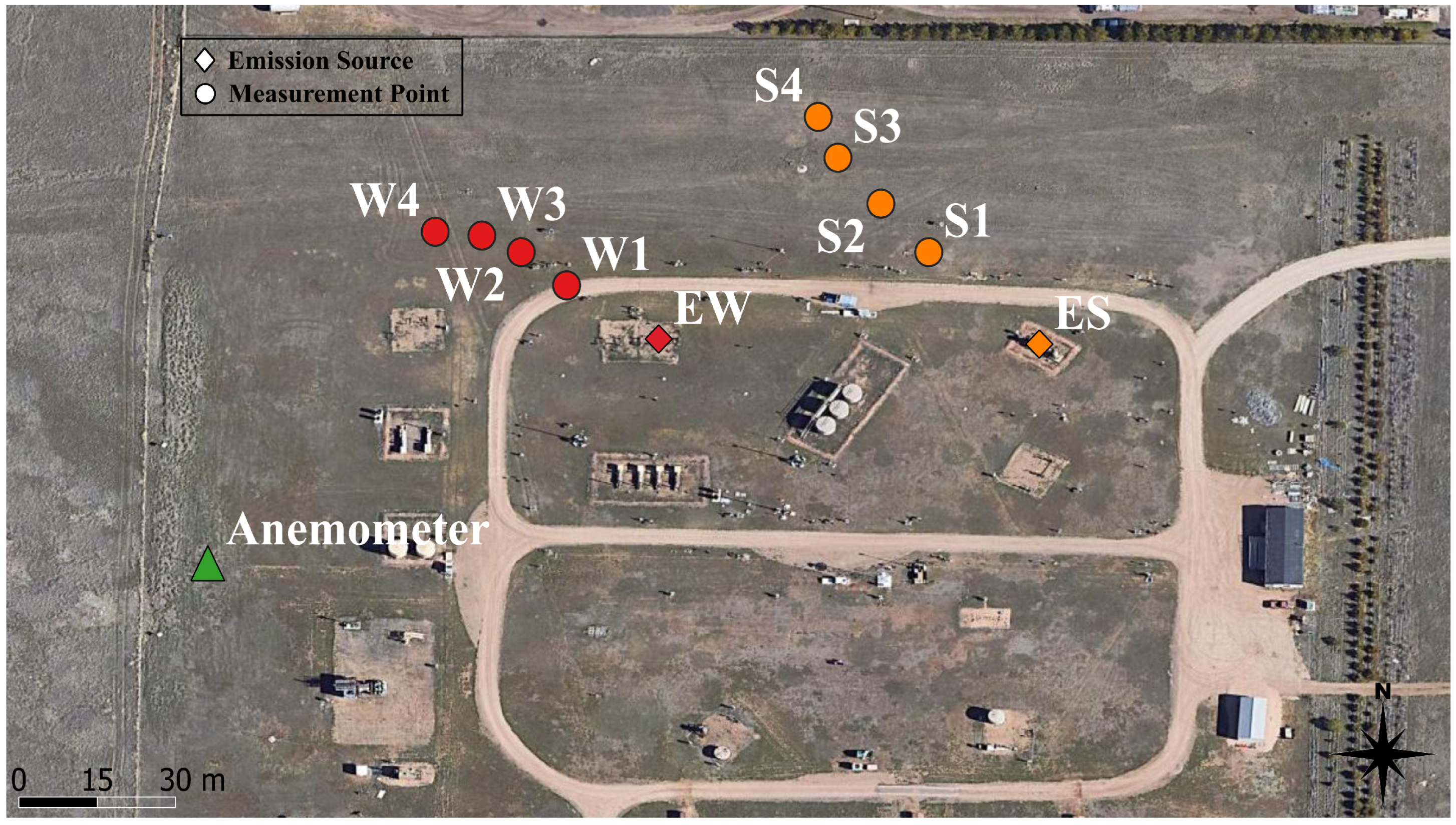
In our study, we performed 2 sets of experiments. The first set of tests was conducted exclusively on pad 5 on 21 March 2024 between 9 and 11 AM and involved the controlled release of 1.3 kg/h $\left[C{H}_4\right]$ from a separator (Figure 1). The second experiment was conducted on 11 July 2024, between 1 and 3 PM on pad 4 on a controlled release of 2.6 kg/h $\left[C{H}_4\right]$ from a wellhead (Figure 1). The equipment on pad 4 and pad 5 varies significantly in size and complexity as obstructions to methane flow, with different release heights. Methane measurements were performed at 4 distances from the release point on both days. In both of these experiments, there was a single-point emission source and a single measurement point with no obstructions between the source and the measurement points other than obstructions caused by the O&G equipment itself. All samples were 4–6 min long. Compressed natural gas was used for emissions, and its composition was determined using gas chromatography.

2.2. Methane Measurements

The methane mixing ratios were measured using a microportable greenhouse gas analyzer (MGGA), a cavity-based spectroscopy instrument built by ABB Technology (Zürich, Switzerland) [29]. The methane concentrations mentioned in the study are denoted as the $C{H}_4$ mixing ratio in ppmv (1 × 10⁻⁶ mol/mol) or simply ppm. The MGGA can measure methane concentration at 1 to 10 Hz with a sensitivity at the ppb level. The reference concentration data for this work were measured at 1 Hz.

The methane measurements were taken in a transect near downwind of the emission source. Methane analyzers were used to measure dry mole mixing ratios downwind of the controlled release using an inlet to the analyzer affixed 1 m above the ground. A Global Positioning Sensor (GPS) marker was used in conjunction with the MGGA to record the exact location of the measurement. The instrument setup used during the field experiments can be seen in Figure S2. The measurement campaign usually ran for one hour to collect 4 samples for each experiment. This allowed us to collect four samples from a single controlled release, each lasting 4 to 6 min. Figure 1 shows the emission source and sensor locations for the 8 samples used in this study.

2.3. Meteorological Data

Meteorological data at 1 Hz were measured using an R. M. Young 3D sonic anemometer (Traverse City, MI, USA) [30] and consisted of temperature, pressure, relative humidity, and wind speed in three directions. The mean wind speed on 21 March 2024 during the data collection period was 2 m/s (between 0.6 and 3.4 m/s) and 3 m/s on 11 July 2024 (between 0.3 and 5.8 m/s). During both measurements, the southeast wind blew between 120 and 150 degrees from the north (Figure S4).

2.4. Wind Modeling

Wind data collected at the METEC were used to create a vertical wind profile between the ground and the height of 15 m using the reference wind speed (u*, m/s) at a height of 6 m, roughness length ($z_0$, m), and von Karman constant (k), as shown in Equation (1) [31]. The roughness length ($z_0$) varies with the surface, and the roughness length in this study was based on the assumed roughness upstream of the releases at the METEC. The von Karman constant is a dimensionless constant (0.4). The same equation is used by Wen et al. [21] to create a vertical wind profile for CFD modeling.

$$\mathrm{u}\left(\mathrm{z}\right)={\displaystyle \frac{u^{\ast }}{k}}log\left({\displaystyle \frac{z}{z_0}}\right)$$

(1)

2.5. CFD Modeling

The methane flow modeling was performed in CONVERGE CFD (Convergent Science, Madison, WI, USA) [32]. We opted for the Reynolds-averaged Navier–Stokes (RANS) approach for turbulence modeling. It is the most common and widespread approach [11,20,21,33]. RANS simulations require the fewest computational resources while still maintaining a good level of accuracy [34] compared to Large-Eddy Simulation (LES) and Direct Numerical Simulation (DNS), the other modeling approaches. The best results can be obtained using DNS since it does not involve flow approximations. However, DNS is computationally inefficient because of its fine spatial and temporal resolution. LES, on the other hand, resolves the larger scales of turbulence explicitly while modeling the smaller scales using subgrid-scale models. This reduces the computational cost compared to DNS while still capturing the essential features of turbulence. LES has been used in some studies, but still has a higher computational cost than the RANS approach [35]. Apart from the computational expense of LES for full-scale environments, there was not enough evidence to justify the use of LES models in this study. Most of the experiments used to validate LES simulations are performed in wind tunnels or under near-ideal conditions [36]. Patnaik et al. [37] reported some degree of reliable prediction using LES for a real site but with great uncertainty. Therefore, the benefits of using LES instead of the RANS approach in simulating outdoor environments are not very well resolved yet, and, in the interest of saving computational expense, we used the RANS approach for our study. For the RANS simulations in this work, boundary conditions (BC) were set for emission inflow and outflow and at other boundaries, i.e., the pipeline, the equipment (tank, separators, pads), and the ground. The BC were usually (1) no-slip solid surfaces internal and external pipelines, (2) wind inflow or outflow, (3) a passive outflow condition at ambient pressure for the outflow boundaries, and (4) the Law of Wall (ground and O&G equipment). More details on the model setup can be found in Table S1, Figure S3a, and Equations (S1)–(S15).

2.6. Meshing

Meshing in CFD is the process of generating a grid of elements to discretize the model domain. The resulting structure is called a mesh. It involves dividing complex geometries into recognizable volumes called elements. CONVERGE CFD requires equipment geometry, and computer-aided design (CAD) models were generated for the METEC equipment using Fusion360 (Autodesk Inc., San Francisco, CA, USA) [38]. It is advantageous, as CONVERGE CFD automatically generates structured orthogonal grids during runtime depending on the input parameters—using fixed embedding or grid scaling—which eliminates manual control of grid size [39,40]. Fixed embedding refines the grids at specific locations in the domain where a finer resolution is critical to the accuracy of the solution. The base grid size in the simulations was 2 m × 2 m × 2 m, and was refined near the surfaces using fixed embedding. Grid scaling refers to changing the size of the base grid between desired events during a simulation, which reduces runtime by coarsening the grids during non-critical simulations and can help capture a critical flow phenomenon by refining the grids at specific times. The total number of grids in the simulation ranged from 100,000 to 300,000 elements.

2.7. Monitoring Points

In the CFD domain, monitoring points were set in 3 dimensions to record the simulated methane concentrations [11,21,23]. Monitoring points are the specific points in the model domain that correspond to the measurement point from the field studies. Five monitoring points were set one meter apart to capture the uncertainty in the sensor location at the measurement point (Figure S3b). The final concentration was calculated as the mean at the 5 points.

2.8. Model Evaluation Metrics

The evaluation of the modeled methane concentration in this research was performed using multiple metrics based on previous studies by Weil et al. [41] and Hanna et al. [42] and summarized by Chang and Hanna [43], and the same approach has been used in many recent papers [17,21,22,25]. The Fractional Bias (FB, Equation (2)) and Geometric Mean Bias (MG, Equation (3)) measure systematic bias, whereas the Geometric Variance (VG, Equation (4)) and Normalized Mean Square Error (NMSE, Equation (5)) measure random scatter. There is no single performance measure that is universally applicable to all situations, and a balanced approach is required to look at a number of performance measures. For dispersion modeling, where concentrations can easily vary by several orders of magnitude, the MG and VG are preferred over the FB and NMSE. However, the MG and VG may be strongly influenced by very low values, and are undefined for zero values. The FAC2 (Equation (6)) is probably the most robust performance measure, because it is not overly influenced by either low or high outliers [43]. A perfect model would have an MG, VG, and FAC2 = 1 and an FB and NMSE = 0. These values are generally not achievable, and the minimum performance measures defined as acceptable summarized by Chang and Hanna [43] are as follows: The fraction of predictions within a factor of two from the observations is about 50% (i.e., FAC2 > 0.5); the mean bias is within ±30% of the mean (−0.3 < FB < 0.3 or 0.7 < MG < 1.3); and the random scatter is about a factor of two within the mean (NMSE < 4 or VG < 1.6).

$$\mathrm{Fractional}\mathrm{Bias}\left(\mathrm{FB}\right)={\displaystyle \frac{Mod-Obs}{0.5\ast (Mod+Obs)}}$$

(2)

$$\mathrm{Geometric}\mathrm{Mean}\mathrm{Bias}\left(\mathrm{MG}\right)=exp(\overline{log\left(Ob{s}_i\right)}-\overline{log\left(Mo{d}_i\right)})$$

(3)

$$\mathrm{Geometric}\mathrm{Variance}\left(\mathrm{VG}\right)=exp(\overline{{(log\left(Ob{s}_i\right)-log\left(Mo{d}_i\right))}^2})$$

(4)

$$\mathrm{Normalize}\mathrm{Mean}\mathrm{Square}\mathrm{Error}\left(\mathrm{NMSE}\right)={\displaystyle \frac{\overline{{(Mod-Obs)}^2}}{\overline{Mod}\ast \overline{Obs}}}$$

(5)

$$\mathrm{Fraction}\mathrm{of}\mathrm{two}\mathrm{of}\mathrm{the}\mathrm{Observations}\left(\mathrm{FAC}2\right)=\mathrm{Fraction}\mathrm{of}\mathrm{data}\mathrm{that}\mathrm{satisfy}0.5\le {\displaystyle \frac{Mod}{Obs}}\le 2$$

(6)

The model evaluation metrics are not exhaustive and model evaluation on additional metrics can be found in the supplement (Tables S2 and S3 and Equations (S16)–(S19)).

2.9. Limitations and Scope of Study

First, there were limitations to the CFD simulations we performed for our study. The limitations were as follows: 1. Pre-existing model physics and suggested parameters were used in all our simulations, but the effects of these parameters on the results were not studied in our work. 2. The mesh was kept coarse to keep the computational time within 24 h on high-performance computing clusters (1 node with 256 GB memory, 64 CPU cores). The base grid size for the simulations varied between 1 and 2 m with grid refinement near the boundaries, e.g., the emission source, ground, equipment vortex, etc. Typically, a finer mesh can provide better simulation results and model convergence but an increased simulation time.

Second, wind modeling (Section 2.4) was performed assuming neutral conditions with a roughness height of 5 cm around the METEC facility. The surface roughness length (z0) in this study was based on the assumed roughness upstream of the releases at the METEC without considering the structures behind the release point. Moreover, the anemometer was not co-located with the emission source or the measurement points. This lack of co-location could have affected the modeled wind speed and turbulence, hence the modeling results [43].

Finally, this study assessed and compared the ability of CFD tools to model external methane flows downwind of a release point. Hence, later, in future studies, detailed post-processing and performance analysis focusing on the impact of variables (such as the underlying model physics, physical parameter values, sensor placement, types of sensors, characteristics of emission points, meteorological conditions, and additional relevant factors) are needed.

3. Results

3.1. Wellhead Experiment

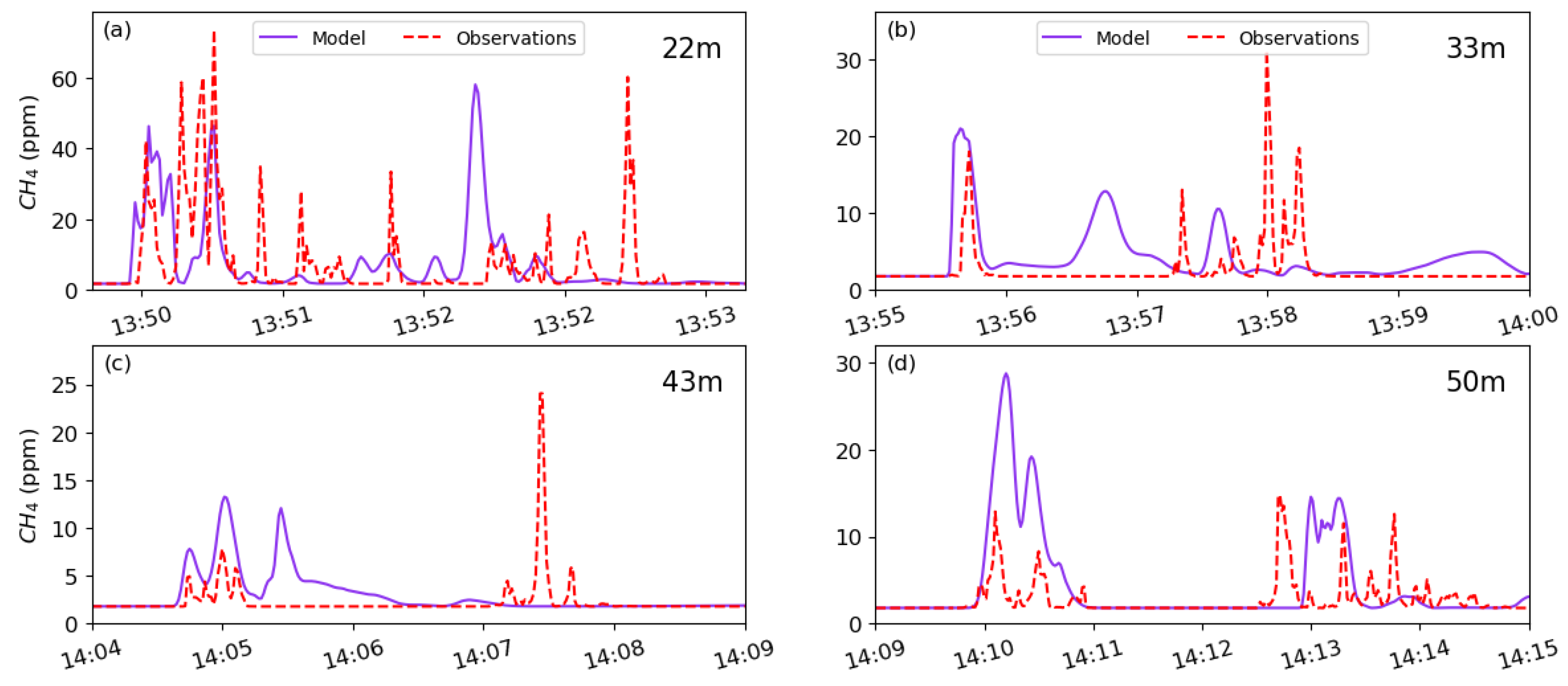
The wellheads were located on pad 4 at the northwest end of the METEC facility (Figure S1). There were five wellheads next to each other from east to west at a separation of 1.5 m, and the methane source was located on the second wellhead from the east. The emission source was positioned at a height of 1.5 m from the ground, and had a release rate of 2.6 kg/h $\left[C{H}_4\right]$. In comparison, the wellhead structure is less complex than the other equipment at the facility. Four measurements were taken downwind of the wellhead, northwest of the source at 22, 33, 43, and 50 m.

CFD Model Performance: Wellhead

The modeled methane concentrations were first evaluated using the metrics summarized by Chang and Hanna [43]. The suggested FAC2 value of 50% or more is a good indicator of the model performance, and the modeled concentrations at all distances had an FAC2 value as high as 0.8 (

Table 1. Fraction of predictions within a factor of 2 of observations (FAC2), Geometric Mean (MG), Geometric Variance (VG), and Normalized Mean Square Error (NMSE) when evaluated against the observed concentration for the wellhead experiment.

Distance (m)	FAC2	MG	VG	NMSE
22	0.58	0.90	3.91	3.26
33	0.60	0.65	2.07	1.80
43	0.80	0.81	1.42	1.27
50	0.75	0.85	1.81	1.40

). MG values for this experiment remained between 0.65 and 0.9, suggesting that the bias was within ±30% of the mean. The NMSE was less than 4; however, the VG values were higher than the suggested value of 1.6 at 22 m and 33 m. The FB in the mean and maximum modeled concentrations at these two distances was within ±40% (Table 1 and

Table 2. Fractional Bias in the maximum modeled concentration for the wellhead experiment (CFD).

Distance (m)	Max. Modeled Concentration (ppm)	Max. Observed Concentration (ppm)	Fractional Bias (%)
22	58.08	73.58	−24
33	21.02	31.18	−38
43	13.25	24.07	−58
50	28.75	14.7	64

). The absolute FB values in the maximum and mean modeled concentrations increased with increasing distance (Table 2 and

Table 3. Fractional Bias in the time-averaged modeled (CFD) concentration for the wellhead experiment.

Distance (m)	Mean Modeled Concentration (ppm)	Mean Observed Concentration (ppm)	Fractional Bias (%)
22	7.62	7.52	2
33	4.24	2.82	40
43	3.01	2.34	26
50	4.36	2.82	42

).

3.2. Separator Experiment

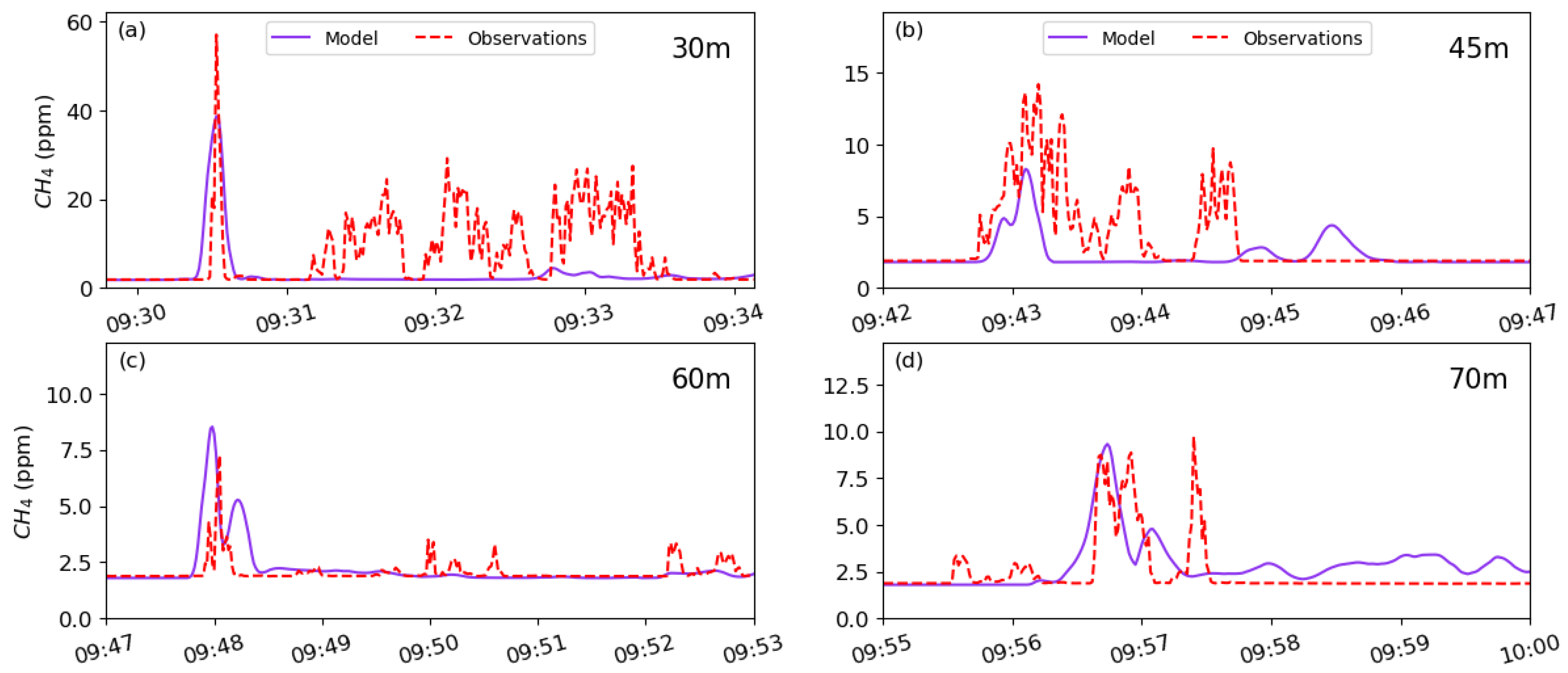
The separators are larger and more complex aerodynamic obstructions located on pad 5 of the METEC facility (Figure S1). There are three separators next to each other and the emission point was 1.7 m from the ground, located between two separators, with a release rate of 1.3 kg/h $\left[C{H}_4\right]$. Methane measurements were taken at 30 m, 45 m, 60 m, and 70 m northwest of the emission source.

CFD Model Performance: Separator

The model performance was satisfactory, with FAC2 values as high as 0.95 and 0.93 at 60 m and 70 m, respectively (

Table 4. Fraction of predictions within a fraction of 2 of observations (FAC2), Geometric Mean (MG), Geometric Variance (VG), and Normalized Mean Square Error (NMSE) when evaluated against observed concentration for the separator experiment.

Distance (m)	FAC2	MG	VG	NMSE
30	0.54	1.96	4.74	3.43
45	0.76	1.27	1.43	0.84
60	0.95	0.98	1.07	0.19
70	0.93	0.84	1.20	0.28

). MG, VG, and FB values adhered well, except at 30 m (Table 4). The model did well in terms of the NMSE, with the values being within 4 at all distances (Table 4). The high MG, VG, and FB values at 30 m suggest a deviation between the model and the observations. A large underestimation by a CFD model is shown in other studies using the k-$ϵ$ model [10]. The absolute Fractional Bias in the maximum modeled concentration stayed between 4% and 54% (

Table 5. Fractional Bias in the maximum modeled concentration for the separator experiment (CFD).

Distance (m)	Max. Modeled Concentration (ppm)	Max. Observed Concentration (ppm)	Fractional Bias (%)
30	38.65	57.02	−38
45	8.28	14.48	−54
60	8.52	7.25	16
70	9.32	9.71	−4

). The values were higher at smaller distances, while dropping to 4% at 70 m (Table 5). This is unlike the wellhead experiment, where it increased with distance. The absolute Fractional Bias in the time-averaged modeled concentration showed a similar trend, with higher values at 30 m and 45 m and drops to 6% and 14% at 60 m and 70 m, respectively (

Table 6. Fractional Bias in time-averaged modeled (CFD) concentration for the separator experiment.

Distance (m)	Mean Modeled Concentration (ppm)	Mean Observed Concentration (ppm)	Fractional Bias (%)
30	3.25	7.7	−82
45	2.31	3.37	−38
60	2.2	2.08	6
70	2.85	2.48	14

). The metrics show that the model performed better farther from the release point.

The CFD modeling results were compared against two controlled-release experiments with different obstruction heights to test how CFD results are affected by aerodynamic complexity. The separator tanks were much larger and wider than the wellhead at the METEC facility. When simulated using the CFD model, we did not see the CFD model performing better than the wellhead experiment or vice versa.

3.3. Gaussian Plume Modeling Results

A Gaussian plume model was run for both the experiments: the controlled release from the wellhead and the release from the separator. The wind data were time-averaged for the experiment duration of 4–6 min for Gaussian modeling. The wind data and the weather conditions were used to determine the PGSC stability class and the dispersion parameters from the look-up table (Table S2). The stability classes for the experiments were either A or B in most of the cases. The results are mentioned in

Table 7. Fractional Bias in the time-averaged modeled (GP) concentration for the wellhead experiment.

Distance (m)	Mean Modeled Concentration (ppm)	Mean Observed Concentration (ppm)	Fractional Bias (%)
22	4.49	7.52	−50
33	1.93	2.82	−38
43	3.09	2.34	28
50	2.22	2.82	−24

and

Table 8. Fractional Bias in the time-averaged modeled (GP) concentration for the separator experiment.

Distance (m)	Mean Modeled Concentration (ppm)	Mean Observed Concentration (ppm)	Fractional Bias (%)
30	3.29	7.70	−80
45	3.60	3.37	−6
60	2.46	2.08	16
70	2.51	2.48	2

.

The Fractional Bias in the Gaussian plume modeled concentration stayed within ±40% for the experiments, except for the two shortest distance, i.e., 22 m and 30 m, where the Gaussian model showed a large underprediction, with biases as high as −50% and −80%. Importantly, the Fractional Bias in the modeled concentration decreased with distance for both the experiments, unlike in the CFD model.

4. Discussion

4.1. CFD Model

The results from the CONVERGE CFD model showed modest agreement with the observations based on the model evaluation metrics (FB, MG, VG, NMSE, FAC2) compared to the results available from similar studies. However, the CFD model in general underestimated the maximum methane concentrations in six of the eight experiments. This was showcased in other studies with constant plume releases [11,15]. The preferred FB values should be within ±30%; however, the FB values ranged between −0.82 and 0.64. This can be compared to Hanna et al.’s [33] −0.32 to 0.6.

CONVERGE CFD is unable to model differentiated gas concentration over time and space, as pointed out in other studies using CFD [11,36]. CONVERGE CFD gave a good description of the average gas concentration while missing the short-term concentration peaks (Figure 2 and Figure 3), leading to large underestimations. This could be attributed to the overall effect of the RANS modeling approach along with the grid size used in this study. With the RANS approach, the flow variables (e.g., velocity) are decomposed into an ensemble mean and a fluctuating term [44]. Studies have suggested that the RANS formulation is inherently incapable of capturing unsteady effects like intermittent separation, eddy generation, and transport [36]. A much finer grid with LES could improve the results as LES better reproduces the mean wind velocity and turbulence kinetic energy [35,45]. However, LES requires high grid refinement, leading to greater computational expense, to properly resolve non-linear interactions at all scales and to obtain meaningful turbulence statistics [46]. In order to capture the fluctuations in the modeled methane concentrations, there is a need for hybrid RANS/LES methods where a near-wall flow is modeled using an RANS approach coupled to an LES model away from the surface [47].

Despite the shortcomings of the RANS approach, with CFD, we could gain insight into the methane flow around complex O&G equipment. The animations based on the results show the methane flow around the separator and wellhead equipment. It is important to analyze how obstructions affect methane flows, which is impossible with Gaussian plume models.

Moreover, a more robust evaluation of the CFD model could not be carried out in this study. Model evaluation of CFD models in previous studies considered huge datasets [14,15,48]. While evaluating the CFD model in [11,15,21] against experiments, only the maximum concentration at each monitoring point was evaluated against the observed concentration. The model results in these studies were not evaluated on a temporal scale. Although these studies serve as the basis for our work, the model evaluation metrics might not provide the best results in our case. The model evaluation in these existing studies is biased towards model performance in predicting maximum concentration, which might diverge significantly from mean concentrations [11].

4.2. Gaussian Plume Model

We also evaluated whether CFD could outperform the simpler Gaussian plume (GP) model for both the wellhead (Table 7) and the separator experiment (Table 8). We found that the GP model performance was better for farther distances and poorer at shorter distances. The big underestimation at shorter distances (22 m, 30 m, and 33 m) is a limitation of Gaussian dispersion models. Studies show that, for unstable conditions (classes A and B) at short distances, the Gaussian model underestimates concentration, and then overestimates at longer distances [49]. Mazzoldi et al. [11] showed a similar trend when evaluating a Gaussian model with Prairie Grass experiments [14]. As discussed in the previous section, a more robust analysis of the Gaussian plume model was not performed here due to limited experimental data. The MG, FAC2, VG, and NMSE metrics were employed with temporal data for the CFD model, which was not possible for the Gaussian plume model.

4.3. CFD vs. Gaussian Model

The biases in the modeled concentrations for the GP were similar to the biases for the CFD model. However, unlike the CFD model, the absolute Fractional Bias in the modeled concentration from the GP had a good linear correlation with distance. The R-value was −0.79, suggesting that the model biases decreased with increasing distance for the Gaussian plume model. For CFD, the R-value for Fractional Biases in the modeled mean concentration with distance was −0.32, showing a weaker correlation. However, the model was evaluated on multiple metrics, and the correlation coefficients with distance are summarized in

Table 9. Correlation coefficient of evaluation metrics with distance for the CFD model.

Evaluation Metric	R-Value
FAC2	0.93
MG	−0.26
VG	−0.77
NMSE	−0.83
FB Max. Concentration (CFD)	0.44
FB Mean Concentration (CFD)	−0.32
FB Mean Concentration (GP)	−0.79

. The FB and MG did not correlate strongly; however, the NMSE and VG correlated well with distance. Hence, we cannot say with certainty if the CFD model performance improves with increasing distance, which is the case with the Gaussian plume model. Hanna et al. [15] showed similar findings, with weak trends in CFD model performance with downwind distance. However, this study had only eight data points, unlike the study of Hanna et al. [15].

Despite a modest agreement between the modeled and measured data, we found two significant shortcomings of the CFD model: the computational expense and the technical expertise required to run the model. The computational time of running CFD models for large domains, such as those used in this study, is very long compared to running the traditional Gaussian plume: hours (6–14 h) compared to seconds. The simulation time depends on domain discretizations, i.e., grid size, time duration, number of steps per second, model physics, solution algorithms, and system approximations [11,15,21].

5. Conclusions

In this work, we studied the utility of a CFD model in modeling methane flows downwind of a methane release at a simulated oil and gas facility. The performance of the CFD model measured by multiple evaluation metrics [33] was in the same range as found in the literature. The FAC2 in all simulations was greater than 0.5, and was the most robust performance metric. The model also performed well in terms of VG and MG, with a few exceptions, while the NMSE values were less than 4 at all distances. FB values were higher than the suggested ±30%, although not very far from the values found in the literature. The results suggest that CFD modeling approaches can be used to generate representative concentrations at a fence line at ∼30 m for oil and gas production equipment with modest success. However, the model was limited in capturing the fine variations in the observations. The results also suggest that the existing results from the CFD model could be improved with good input data, optimized parameters with an improved grid size, and a better modeling approach, such as hybrid RANS-LES. From this limited comparison, there does not appear to be a bias caused by the aerodynamic complexity of the emission point. The model did not perform better selectively for the wellhead or separator experiments, despite one being more complex than the other.

Although the results of the CFD modeling were satisfactory, the Gaussian plume model was able to capture the mean concentration with Fractional Biases in the same range as the CFD model. We suggest that the demands of running the CFD (computational time and technical expertise) mean that CFD is unlikely to replace the current atmospheric dispersion models, like the Gaussian plume, when rapid responses are required until the models are simplified or computers run much faster. However, this work, along with the existing literature, makes a strong case for CFD to be used in designing, developing, and studying O&G facilities, not only for hazardous studies but also for studying methane flows in a complex space.

References

1. U.S. Environmental Protection Agency (EPA). Global Greenhouse Gas Overview. 2024. Available online: https://www.epa.gov/ghgemissions/global-greenhouse-gas-overview (accessed on 29 October 2024).
2. U.S. Environmental Protection Agency. Inventory of US Greenhouse Gas Emissions and Sinks: 1990–2020 (EPA, 2024). 2024. Available online: https://www.epa.gov/ghgemissions/inventory-us-greenhouse-gas-emissions-and-sinks (accessed on 29 October 2024).
3. U.S. Energy Information Administration (EIA). Natural Gas and the Environment. 2025. Available online: https://www.eia.gov/energyexplained/natural-gas/natural-gas-and-the-environment.php (accessed on 17 January 2025).
4. Mbua, M.; Riddick, S.N.; Kiplimo, E.; Zimmerle, D. Evaluating the accuracy of downwind methods for quantifying point source emissions. EGUsphere 2024. preprint. [Google Scholar] [CrossRef]
5. Riddick, S.N.; Mbua, M.; Riddick, J.C.; Houlihan, C.; Hodshire, A.L.; Zimmerle, D.J. A cautionary report of calculating methane emissions using low-cost fence-line sensors. Elem. Sci. Anthr. 2022, 10, 00021. [Google Scholar] [CrossRef]
6. National Aeronautics and Space Administration, Glenn Research Center. Navier-Stokes Equation. Available online: https://www1.grc.nasa.gov/beginners-guide-to-aeronautics/navier-strokes-equation/ (accessed on 18 September 2024).
7. Petersen, R.L. Effect of homogeneous and heterogeneous surface roughness on heavier-than-air gas dispersion. J. Wind Eng. Ind. Aerodyn. 1990, 36, 643–652. [Google Scholar] [CrossRef]
8. Wang, H.; Liu, B.; Liu, X.; Lu, C.; Deng, J.; You, Z. Dispersion of CO2 released from buried high-pressure pipeline over complex terrain. Environ. Sci. Pollut. Res. 2021, 28, 6635–6648. [Google Scholar] [CrossRef]
9. Xing, J.; Liu, Z.; Huang, P.; Feng, C.; Zhou, Y.; Zhang, D.; Wang, F. Experimental and numerical study of the dispersion of CO2 plume. J. Hazard. Mater. 2013, 256–257, 40–48. [Google Scholar] [CrossRef]
10. Sklavounos, S.; Rigas, F. Validation of turbulence models in heavy gas dispersion over obstacles. J. Hazard. Mater. 2004, 108, 9–20. [Google Scholar] [CrossRef] [PubMed]
11. Mazzoldi, A.; Hill, T.; Colls, J. CFD and Gaussian atmospheric dispersion models: A comparison for leak from CO2 transportation and storage facilities. Atmos. Environ. 2008, 42, 8046–8054. [Google Scholar] [CrossRef]
12. Fluidyn-Panache—CFD Software for Air Quality and Gas Dispersion. 2025. Available online: https://www.fluidyn.com/fluidyn-consultancy-software-cfd-multiphysics-11/fluidyn-panache/ (accessed on 17 March 2025).
13. United States Environmental Protection Agency. ALOHA Software. 2025. Available online: https://www.epa.gov/cameo/aloha-software (accessed on 17 March 2025).
14. Laboratory, A.A. Project Prairie Grass, a Field Program in Diffusion: Volume 1; Geophysical Research Papers; US Air Force Cambridge Research Center: Bedford, MA, USA, 1958. [Google Scholar]
15. Hanna, S.R.; Chang, J.C. Use of the Kit Fox field data to analyze dense gas dispersion modeling issues. Atmos. Environ. 2001, 35, 2231–2242. [Google Scholar] [CrossRef]
16. Schleder, A.M.; Martins, M.R. Experimental data and CFD performance for CO2 cloud dispersion analysis. J. Loss Prev. Process Ind. 2016, 43, 688–699. [Google Scholar] [CrossRef]
17. Toja-Silva, F.; Chen, J.; Hachinger, S.; Hase, F. CFD simulation of CO2 dispersion from urban thermal power plant: Analysis of turbulent Schmidt number and comparison with Gaussian plume model and measurements. J. Wind Eng. Ind. Aerodyn. 2017, 169, 177–193. [Google Scholar] [CrossRef]
18. OpenFOAM. 2025. Available online: https://www.openfoam.com/ (accessed on 17 March 2025).
19. Tan, W.; Li, C.; Wang, K.; Zhu, G.; Wang, Y.; Liu, L. Dispersion of CO2 plume in street canyons. Process Saf. Environ. Prot. 2018, 116, 235–242. [Google Scholar] [CrossRef]
20. Wareing, C.J.; Fairweather, M.; Falle, S.A.E.G.; Woolley, R.M. Validation of a model of gas and dense phase CO2 jet releases for carbon capture and storage application. Int. J. Greenh. Gas Control 2014, 20, 254–271. [Google Scholar] [CrossRef]
21. Wen, J.; Heidari, A.; Xu, B.; Jie, H. Dispersion of CO2 from vertical vent and horizontal releases—A numerical study. Proc. Inst. Mech. Eng. Part E J. Process Mech. Eng. 2013, 227, 125–139. [Google Scholar] [CrossRef]
22. Wen, J.X.; Fur, P.L.; Jie, H.; Vendra, C.M.R. Further development and validation of CO2FOAM for the atmospheric dispersion of accidental releases from CO2 pipelines. Int. J. Greenh. Gas Control 2016, 52, 293–304. [Google Scholar] [CrossRef]
23. Liu, B.; Liu, X.; Lu, C.; Godbole, A.; Michal, G.; Tieu, A.K. Computational fluid dynamics simulation of CO2 dispersion in a complex environment. J. Loss Prev. Process Ind. 2016, 40, 419–432. [Google Scholar] [CrossRef]
24. Ansys Fluent|Simulation Software. 2025. Available online: https://www.ansys.com/products/fluids/ansys-fluent (accessed on 17 March 2025).
25. Joshi, P.; Bikkina, P.; Wang, Q. Consequence analysis of accidental release of supercritical CO2 from high-pressure pipelines. Int. J. Greenh. Gas Control 2016, 55, 166–176. [Google Scholar] [CrossRef]
26. Colorado State University. METEC|Colorado State University. 2024. Available online: https://metec.colostate.edu/ (accessed on 2 September 2024).
27. Day, R.E.; Emerson, E.; Bell, C.; Zimmerle, D. Point Sensor Networks Struggle to Detect and Quantify Short Controlled Releases at Oil and Gas Sites. Sensors 2024, 24, 2419. [Google Scholar] [CrossRef]
28. Riddick, S.N.; Mbua, M.; Riddick, J.C.; Houlihan, C.; Hodshire, A.L.; Zimmerle, D.J. Uncertainty Quantification of Methods Used to Measure Methane Emissions of 1 g CH4 h-1. Sensors 2023, 23, 9246. [Google Scholar] [CrossRef]
29. Microportable Greenhouse Gas Analyser, (MGGA). 2018. Available online: https://www.sol-ma.net/wp-content/uploads/2018/07/DS_LGR-ICOS_MGGA-EN-Rev.-C.pdf (accessed on 19 September 2024).
30. R. M. Young Company. Wind Monitor. Available online: https://www.youngusa.com/product/wind-monitor/ (accessed on 14 February 2025).
31. Seinfeld, J.H.; Pandis, S.N. Atmospheric Chemistry and Physics: From Air Pollution to Climate Change, 2nd ed.; J. Wiley: Hoboken, NJ, USA, 2006. [Google Scholar]
32. CONVERGE CFD. Available online: https://convergecfd.com (accessed on 17 January 2025).
33. Hanna, S.R.; Hansen, O.R.; Dharmavaram, S. FLACS CFD air quality model performance evaluation with Kit Fox, MUST, Prairie Grass, and EMU observations. Atmos. Environ. 2004, 38, 4675–4687. [Google Scholar] [CrossRef]
34. Caron, C.; Lauret, P.; Bastide, A. Machine Learning to speed up CFD engineering simulations for built environments: A review. Build. Environ. 2025, 267, 112229. [Google Scholar] [CrossRef]
35. Nozu, T.; Tamura, T. LES of turbulent wind and gas dispersion in a city. J. Wind Eng. Ind. Aerodyn. 2012, 104–106, 492–499. [Google Scholar] [CrossRef]
36. Sumner, J.; Watters, C.S.; Masson, C. CFD in Wind Energy: The Virtual, Multiscale wind tunnel. Energies 2010, 3, 989–1013. [Google Scholar] [CrossRef]
37. Patnaik, G.; Boris, J.P.; Young, T.R.; Grinstein, F.F. Large Scale Urban Contaminant Transport Simulations with Miles. J. Fluids Eng. 2007, 129, 1524–1532. [Google Scholar] [CrossRef]
38. Autodesk. Autodesk Fusion|3D CAD, CAM, CAE, and PCB Cloud-Based Software. 2025. Available online: https://www.autodesk.com/products/fusion-360 (accessed on 17 January 2025).
39. Hockett, A.; Hampson, G.; Marchese, A.J. Development and Validation of a Reduced Chemical Kinetic Mechanism for CFD Simulations of Natural Gas/Diesel Dual-Fuel Engines. Energy Fuels 2016, 30, 2414–2427. [Google Scholar] [CrossRef]
40. Gupta, S.K.; Mittal, M. Analysis of Cycle-To-Cycle Combustion Variations in a Spark-Ignition Engine Operating under Various Biogas Compositions. Energy Fuels 2019, 33, 12421–12430. [Google Scholar] [CrossRef]
41. Weil, J.C.; Sykes, R.I.; Venkatram, A. Evaluating air-quality models: Review and outlook. J. Appl. Meteorol. Climatol. 1992, 31, 1121–1145. [Google Scholar] [CrossRef]
42. Hanna, S.R.; Chang, J.C.; Strimaitis, D.G. Hazardous gas model evaluation with field observations. Atmos. Environ. 1993, 27, 2265–2285. [Google Scholar] [CrossRef]
43. Chang, J.C.; Hanna, S.R. Air quality model performance evaluation. Meteorol. Atmos. Phys. 2004, 87, 167–196. [Google Scholar] [CrossRef]
44. CONVERGE CFD. CONVERGE 3.0 Manual. Available online: https://convergecfd.com (accessed on 17 January 2025).
45. Tominaga, Y.; Mochida, A.; Murakami, S.; Sawaki, S. Comparison of various revised k–ϵ models and LES applied to flow around a high-rise building model with 1:1:2 shape placed within the surface boundary layer. J. Wind Eng. Ind. Aerodyn. 2008, 96, 389–411. [Google Scholar] [CrossRef]
46. Wood, N. Wind Flow over Complex Terrain: A Historical Perspective and the Prospect for Large-Eddy Modelling. Bound.-Layer Meteorol. 2000, 96, 11–32. [Google Scholar] [CrossRef]
47. Bechmann, A.; Sørensen, N. Hybrid RANS/LES Method for Wind Flow over Complex Terrain. Wind Energy Int. J. Prog. Appl. Wind Power Convers. Technol. 2010, 13, 36–50. [Google Scholar] [CrossRef]
48. Biltoft, C.A. Customer Report for Mock Urban Setting Test; U.S. Army Developmental Test Command: Aberdeen Proving Ground, MD, USA, 2001. [Google Scholar]
49. Dharmavaram, S.; Hanna, S.R.; Hansen, O.R. Consequence analysis using a CFD model for industrial sites. Process Saf. Prog. 2005, 24, 316-272. [Google Scholar] [CrossRef]
Figure 1. Schematic of the emission source and sensor location at METEC for the controlled-release experiments. W1 to W4 are measurements taken from wellhead emissions, and S1 to S4 are measurements taken from separator emissions. The anemometer’s location is shown in green.
Atmosphere 16 00811 g001
Figure 2. Modeled methane concentration plotted against observations for release from the wellhead on 11 July 2024 at 4 distances (ad). The y-axis shows the methane concentration, with time displayed in hours and minutes.
Atmosphere 16 00811 g002
Figure 3. Modeled methane concentration plotted against observations for the release from the separator on 21 March 2024 at 4 distances (ad). The y-axis shows the methane concentration, with time displayed in hours and minutes.
Atmosphere 16 00811 g003