High-Resolution Daily XCH₄ Prediction Using New Convolutional Neural Network Autoencoder Model and Remote Sensing Data

Abstract

Atmospheric methane (CH₄) concentrations have increased to 2.5 times their pre-industrial levels, with a marked acceleration in recent decades. CH₄ is responsible for approximately 30% of the global temperature rise since the Industrial Revolution. This growing concentration contributes to environmental degradation, including ocean acidification, accelerated climate change, and a rise in natural disasters. The column-averaged dry-air mole fraction of methane (XCH₄) is a crucial indicator for assessing atmospheric CH₄ levels. In this study, the Sentinel-5P TROPOMI instrument was employed to monitor, map, and estimate CH₄ concentrations on both regional and global scales. However, TROPOMI data exhibits limitations such as spatial gaps and relatively coarse resolution, particularly at regional scales or over small areas. To mitigate these limitations, a novel Convolutional Neural Network Autoencoder (CNN-AE) model was developed. Validation was performed using the Total Carbon Column Observing Network (TCCON), providing a benchmark for evaluating the accuracy of various interpolation and prediction models. The CNN-AE model demonstrated the highest accuracy in regional-scale analysis, achieving a Mean Absolute Error (MAE) of 28.48 ppb and a Root Mean Square Error (RMSE) of 30.07 ppb. This was followed by the Random Forest (RF) regressor (MAE: 29.07 ppb; RMSE: 36.89 ppb), GridData Nearest Neighbor Interpolator (NNI) (MAE: 30.06 ppb; RMSE: 32.14 ppb), and the Radial Basis Function (RBF) Interpolator (MAE: 80.23 ppb; RMSE: 90.54 ppb). On a global scale, the CNN-AE again outperformed other methods, yielding the lowest MAE and RMSE (19.78 and 24.7 ppb, respectively), followed by RF (21.46 and 27.23 ppb), GridData NNI (25.3 and 32.62 ppb), and RBF (43.08 and 54.93 ppb).

1. Introduction

Methane (CH₄) is one of the most potent greenhouse gases, contributing significantly to global warming, and the column-averaged dry-air mole fraction of atmospheric CH₄ (XCH₄) is a vital parameter in assessing atmospheric methane concentrations. As methane has a higher global warming potential compared to carbon dioxide over short timescales, addressing CH₄ emissions is critical to mitigating climate change. Effective measures to tackle this issue include reducing methane emissions, advancing low-carbon technologies, implementing methane capture and storage solutions, and supporting related research activities [1,2].

CH₄ emissions fall into three categories: (1) human accidental emissions from industrial leaks and pipeline failures, (2) natural human-caused emissions from activities like livestock farming and rice cultivation, and (3) natural emissions from wetlands, permafrost, and geological seepage. Understanding these distinctions is crucial for effective climate strategies and methane forecasting models [3].

In its sixth assessment report, the Intergovernmental Panel on Climate Change (IPCC) emphasized the role of human activities, including fossil fuel extraction, agriculture, and waste management, in driving methane emissions. This underscores the importance of methane monitoring and estimation research as a priority for global climate action [4].

Remote sensing technologies play a pivotal role in monitoring XCH₄ globally, repeatedly, and with greater efficiency compared to traditional methods such as ground stations, handheld sensors, or localized monitoring using tethered balloons. Dedicated satellites for methane monitoring include the TROPOMI instrument onboard the Sentinel-5P satellite [5], the GOSAT satellite series (Tsukuba, Japan) [6,7], and methane monitoring missions like GHGSat (Montreal, QC, Canada) [8]. Despite these advancements, challenges remain in remote sensing methodologies:

Low Temporal Resolution: Instruments such as GOSAT and Sentinel-5P often require extended periods (e.g., 16 days for GOSAT) to revisit specific areas, resulting in gaps in spatial coverage. Moreover, these satellites can have information gaps due to cloud cover, sensor limitations, or orbital constraints, necessitating the use of interpolation techniques for generating complete datasets.

To address these challenges, Jiang et al. [9] combined Data Interpolation Empirical Orthogonal Function (DINEOF) [10] with Bayesian Maximum Entropy (BME), achieving high accuracy in reconstructing missing XCH₄ data for large regions based on monthly averages.

Wefers et al. [11] introduced a methodology called XCH₄SAT+ to analyze long-term trends in XCH₄ across selected European sites. This approach leveraged data from multiple satellite missions, combining them through statistical interpolation techniques to enhance temporal and spatial coverage. To ensure reliability, the method underwent validation against measurements from European TCCON (Total Carbon Column Observing Network) stations. However, its broader applicability was constrained by the availability and consistency of input data, limiting the scope of its implementation.

Hu et al. [12] utilized Channel Attention Mechanism (CAM) [13] and Long Short-Term Memory (LSTM) [14] to predict missing methane data derived from OCO-2 observations. While the method showed promising results for summer datasets, its performance in winter was less robust. Sheng et al. [15] applied spatiotemporal kriging [16] using data from GOSAT and OCO-2 between 2009 and 2020 to address gaps across a global grid with a one-degree resolution and a three-day interval. Their approach effectively resolved data inconsistencies over large areas. Zhang et al. [17] used XGBoost to retrieve XCH4 from Sentinel-5p TROPOMI L2 and compared it to the one produced by the European Space Agency (ESA), and they were, according to the authors, approximately comparable.

Remote sensing of XCH₄ remains a critical avenue for advancing our understanding of methane dynamics and mitigating its climate impacts. Integrating innovative modelling techniques and leveraging multi-satellite datasets will be essential for addressing data gaps and improving the reliability of methane monitoring systems. In the literature, many attempts exist to fill the gaps in the existing remote sensing data provided by the current XCH₄ satellites. However, the literature exhibits several weaknesses in addressing these problems. These include the following: (1) coverage is limited to large, global areas; (2) selection of long analysis periods; (3) use of heterogeneous satellites; (4) application of conventional interpolation methods.

In this research, we addressed all the aforementioned problems by experimenting with both large and small regional study areas. We utilized data from Sentinel-5P TROPOMI. We analyzed one day and compared various interpolation and prediction methods. Additionally, we employed efficient verification techniques based on a specific number of TCCON stations within the study area. To achieve these tasks, we wrote numerous scripts in Python version 3.11.13 and Java 21 using the Google CoLab [18] and Google Earth Engine (GEE) [19] platforms.

2. Materials and Methods

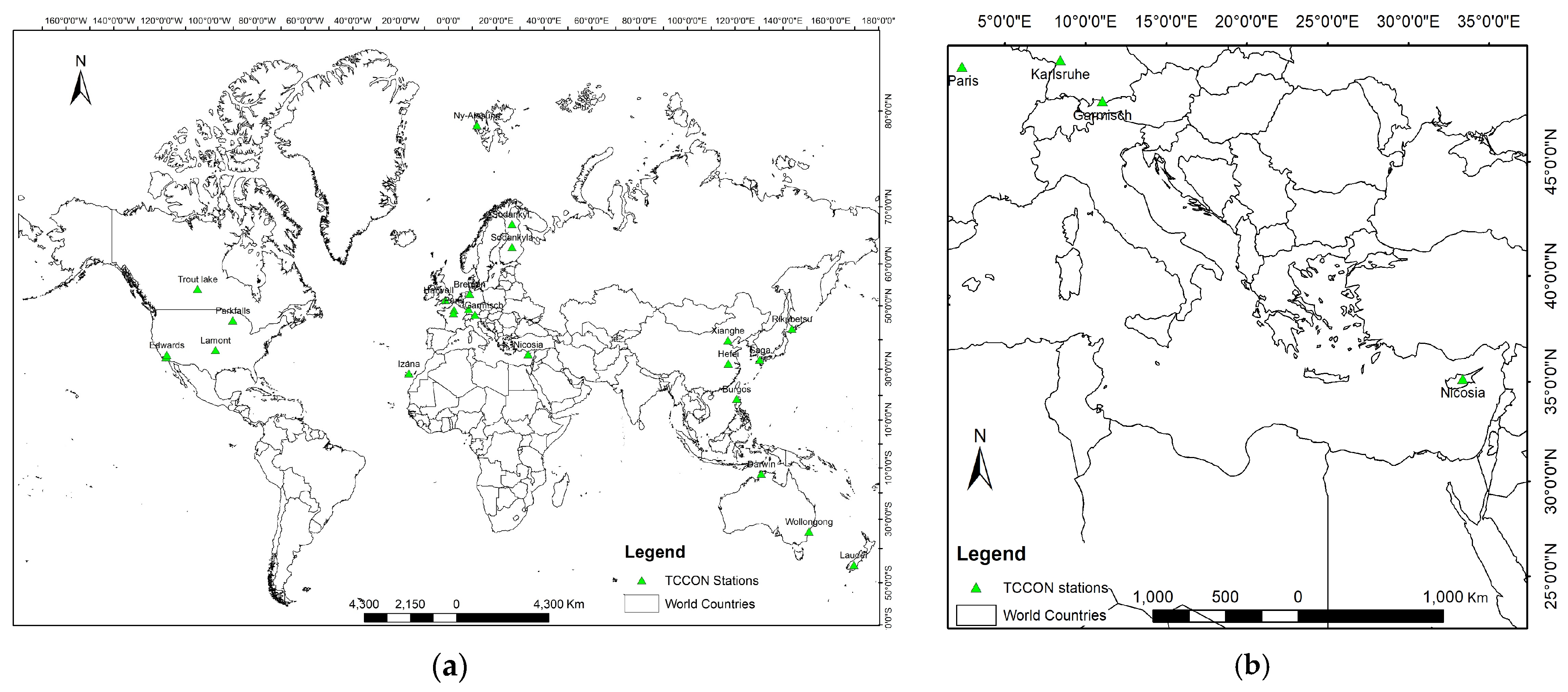
2.1. Materials

In this research, we deployed Sentinel-5P TROPOMI to monitor, estimate, and map XCH₄ in different study areas. The Sentinel-5 Precursor (Sentinel-5P) satellite, launched by the European Space Agency (ESA) in October 2017, is equipped with the Tropospheric Monitoring Instrument (TROPOMI). This advanced instrument is designed to monitor atmospheric trace gases, including CH₄, with high precision and resolution. Below is a detailed overview, focusing on its capabilities for CH₄ monitoring:

XCH₄ Monitoring: TROPOMI measures the column-averaged dry-air mole fraction of methane (XCH₄) using absorption information from the Shortwave Infrared (SWIR) spectral range and the Oxygen-A Band (760 nm). This allows for high sensitivity to methane concentrations near the Earth’s surface [20].

Spatial and Temporal Resolution: TROPOMI offers a spatial resolution of up to 7 km × 5.5 km, making it capable of detecting localized methane sources, such as emissions from agriculture, landfills, and fossil fuel extraction [20]. The instrument provides global coverage with a revisit time of approximately one day, enabling near-real-time monitoring of methane emissions and concentrations.

Methane data from TROPOMI is available as Level 2 (geolocated) products, which are processed to provide total column methane concentrations. These datasets are accessible through platforms like the Copernicus Open Access Hub [20].

Many challenges are encountered the users of Sentinel-5P, such as methane retrievals are affected by cloud cover, which can obscure measurements. Moreover, despite its high resolution, some gaps in data may occur due to instrument limitations or adverse atmospheric conditions (Figure 1). One can easily notice the gaps (white) on land and oceans, although the data covers complete months. Interpolation techniques are often used to address these gaps.

Also, CH₄ concentrations in 2019 were very high in North Africa, the Middle East, and South and East Asia compared to other regions in the world. Moreover, notice that as the temperature gets high, the CH₄ emission increases at the poles.

The downloaded data was for the year 2019 for a study area that encompasses a large area in the Mediterranean basin. We selected a specific year to ensure that Sentinel-5P data is available, and to show the variations in XCH₄ during different seasons. Also, a need arose to study two different years, 2019 and 2021, to discover trends in the XCH₄ emission increase. Certain intervals within the selected years were carefully analyzed and utilized to estimate the column-averaged dry-air mole fraction of methane (XCH₄). These periods were chosen based on their data quality, coverage, and relevance to the study objectives, ensuring robust and reliable methane estimations. Sentinel-5p TROPOMI covers the whole globe. So, in this research, we used different study areas. One covered the longitudes from 180° W to 180° E and latitudes from 90° S to 90° N. The second small regional area, spanning longitudes from 1° E to 40° E and latitudes from 20° N to 50° N, was selected due to its geographical significance and relevance to the study objectives (Figure 2a,b). This region includes diverse environmental conditions and anthropogenic influences, making it valuable for analyzing XCH₄ concentration variations. The use of high-resolution interpolation in this area helps reveal fine-scale spatial variations.

Several steps were implemented to create unified, good-quality, and non-redundant data. These steps are explained in detail in Section 2.2. In the first study area, we used 25 stations that cover the Earth. These stations are Sodankylä, Paris, Nicosia, Izana, Garmisch, Karlsruhe, Breman, Burgos, Caltech, Darwin, Trout Lake, Edwards, Garmisch, Hefei, Harwell, Lauder, Lamont, Ny-Alesund, Orleans, Parkfalls, Rikubetsu, Saga, Sodankyla, Wollongong, and Xianghe (Figure 2a). These stations are located on every continent and can provide a good source of information. In the second area of study, five different Total Carbon Column Observing Network (TCCON) stations were used to cover the area and verify the interpolated XCH₄ values using different methods. These stations are Paris, Nicosia, Garmisch, Orleans, and Karlsruhe (Figure 2b).

2.2. Methods

The methods were implemented to acquire, modify, analyze, interpolate, and display XCH₄ data from a reliable satellite, Sentinel-5P. The complete processes are shown in the following graph (Figure 3).

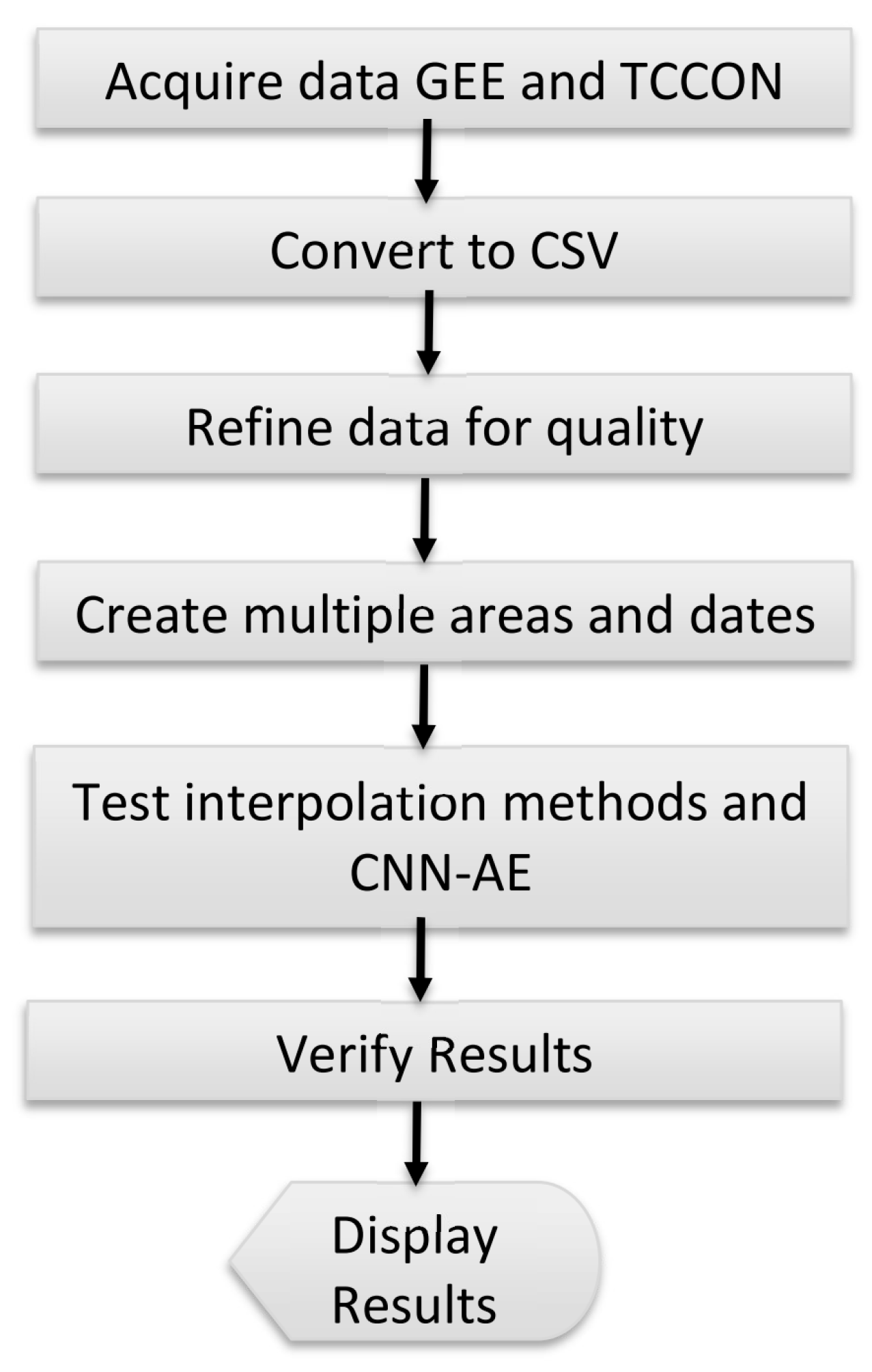
2.2.1. Acquire Data Using Google Earth Engine (GEE)

Google Earth Engine (GEE) is authenticated through user login credentials tied to a registered Google account. Once authenticated, users gain access to its vast computational and data resources. A JavaScript was developed to automate these steps and verify the presence of the necessary data.

For the extraction of data, GEE hosts an extensive repository, including satellite datasets like Sentinel-5P, which contains atmospheric observations, including methane concentration bands. The extraction begins by filtering this dataset based on temporal and spatial parameters, such as a specified date range and region of interest. The data is then processed by applying operations like clipping, mosaicking, or aggregating images to create meaningful outputs tailored to research goals. These processed outputs can be analyzed further through sampling or spatial interpolation techniques and visualized directly within GEE’s Map platform using customizable color palettes and styles. This workflow ensures seamless integration from data extraction to display, empowering users with insights derived from environmental data.

2.2.2. Testing Interpolation Techniques and Building the CNN-AE Model

In this subsection, the models are briefly introduced. The reader should refer to the literature in each subsection below for more details.

I 

Radial Basis Function (RBF)

The Radial Basis Function (RBF) model can provide excellent interpolants for high-dimensional datasets of poorly distributed data points (scarce and unevenly distributed points). For any finite dataset in any Euclidean space, one can construct an interpolation of the data using RBFs, even if the data points are unevenly and sporadically distributed in a high-dimensional Euclidean space [21].

Let $f\left(x\right)$ be a real-valued function of the input vector $x$ defined on a subset Ω of ${\mathbb{R}}^n$ such that the value of f at N input vectors $x^j$, j = 1,…, N, ${f(x}^j)$ is given. The goal is to construct an estimation model $g\left(x\right)$ such that ${g(x}^j)={f(x}^j)$ for j = 1,…, N. The interpolation requirement can be satisfied by RBF interpolation. Interpolation functions generated from an RBF $\phi \left(t\right)$ can be represented in the following form:

$$g\left(x\right)={\sum }_{j=1}^N{\alpha }_j\phi (||x-x^j||),$$

(1)

where $\left|\right|x-x^j\left|\right|$ denotes the parameterized distance between $x$ and $x^j$. The most popular examples of RBF [22] are cubic spline $\phi \left(t\right)=t^3$, thin plate spline $\phi \left(t\right)=t^2\mathrm{l}\mathrm{n}\left(t\right)$, multiquadric $\phi \left(t\right)=\sqrt{1+t^2}$, and Gaussian $\phi \left(t\right)=\mathrm{e}\mathrm{x}\mathrm{p}(-t^2$).

II 

Overview of Interpolation Algorithms in SciPy GridData

GridData is a function in the SciPy library used for interpolating unstructured, multidimensional data [23]. It is particularly useful when there are scattered data points and values must be estimated at intermediate points. The function supports several interpolation methods, each with its theoretical basis:

Nearest Neighbor Interpolation (NNI) assigns the value of the nearest data point to the interpolation point. It is based on the Voronoi diagram, where each interpolation point is assigned the value of the closest data point (Equation (2)). NNI is simple and fast but can produce discontinuities.

$$f\left(x\right)=f\left(x_{nearest}\right)$$

(2)

Linear interpolation (LI) performs linear interpolation within the Delaunay triangulation of the input points (Equation (3)). The Delaunay triangulation divides the convex hull of the input points into non-overlapping simplices (triangles in 2D, tetrahedra in 3D, etc.). Linear interpolation is then performed within each simplex. LI provides a balance between computational efficiency and smoothness.

$$f\left(x\right)={\sum }_{i=1}^{n+1}{\lambda }_{i}f\left(x_i\right)where{\sum }_{i=1}^{n+1}{\lambda }_i=1$$

(3)

Linear interpolation within a simplex (triangle in 2D, tetrahedron in 3D) formed by the Delaunay triangulation. The weight (${\lambda }_i$) is the barycentric coordinate of the point $f\left(x\right)$ within the simplex.

Among the various interpolation methods available in SciPy’s GridData, NNI was selected for this study due to its ability to 1—preserve discrete values: since methane concentration data might come from satellite retrievals or discrete sensor measurements, NNI ensures that interpolated values remain exactly as observed rather than smoothed; 2—avoid artificial gradients: linear interpolation introduces gradual transitions between points, which can artificially smooth out concentration hotspots, potentially misrepresenting true variations; 3—facilitate greater stability for irregular data: satellite data or in situ observations can have uneven spatial distribution, meaning linear interpolation might distort values in areas with sparse measurements; 4—provide computational efficiency: NNI is faster, avoiding the weighted averaging calculations involved in linear methods.

III 

Random Forest Regression Method

Random Forest Regression (RF) is an ensemble learning technique that combines multiple decision trees to improve predictive accuracy and reduce overfitting. Unlike a single decision tree, which may be prone to variance and bias, Random Forest builds multiple trees using different subsets of the data and averages their predictions to produce a more stable and reliable output [24].

RF Regression works as follows: 1—Bootstrap Sampling: the algorithm selects random subsets of the training data with replacement; 2—Decision Tree Construction: each subset is used to train an individual decision tree; 3—Feature Selection: at each split, a random subset of features is considered to ensure diversity among trees; 4—Prediction Aggregation: for regression, the final prediction is the average of all tree outputs.

Given a set of decision trees T₁, T₂, …, T_n the Random Forest Regression prediction $\widehat{y}$ for an input $x$ is computed as Equation (4):

$$\widehat{y}={\displaystyle \frac{1}{n}}{\sum }_{i=1}^n{T}_i\left(x\right)$$

(4)

One should note that the predicted points by RF can be used to create a grid based on any kernel, such as NNI or LI.

IV 

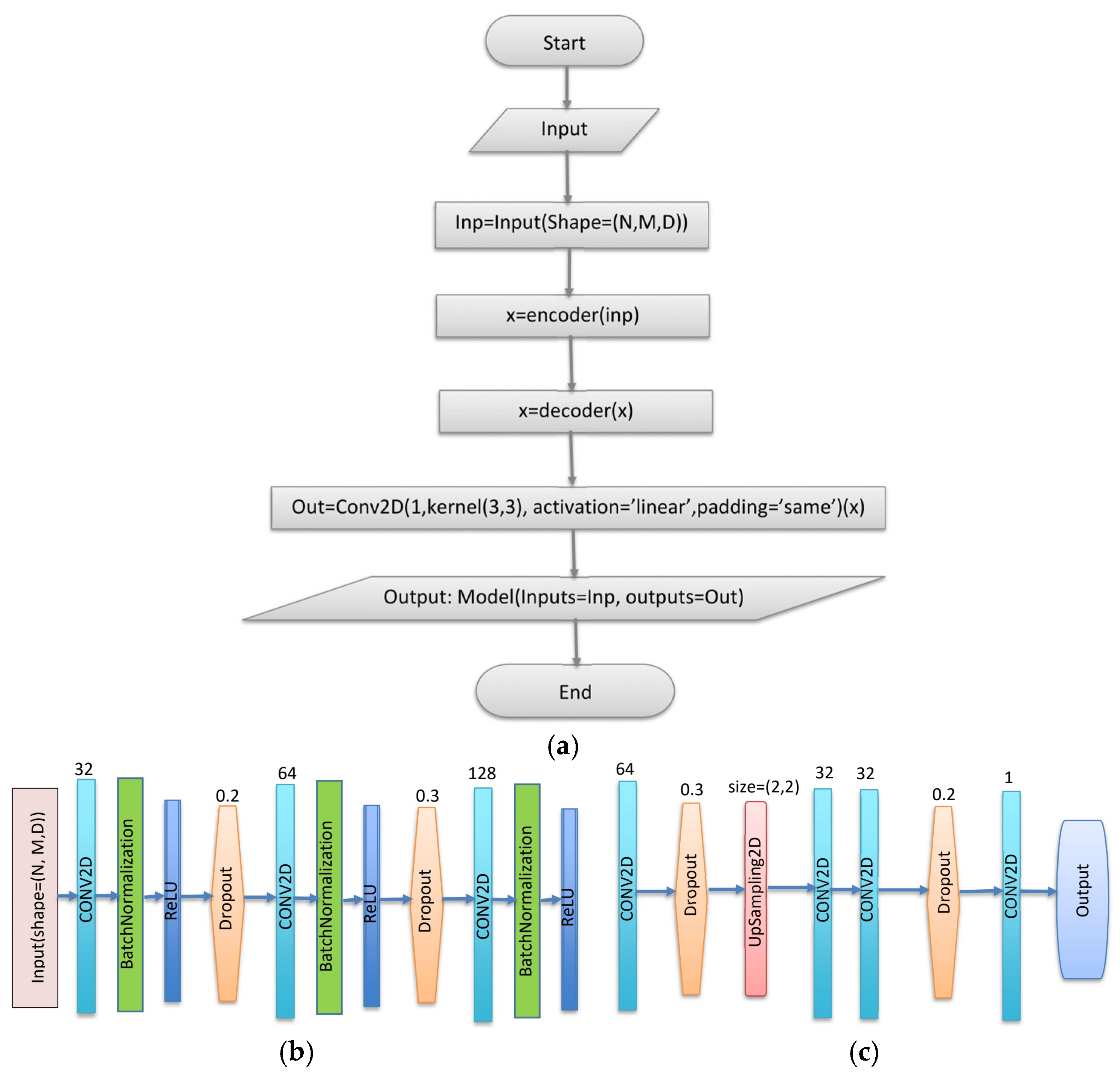
A New CNN Autoencoder (CNN-AE) Model for the Prediction of XCH₄

This Autoencoder CNN consists of two main parts: the encoder and decoder, each containing specific components designed for feature extraction and reconstruction. The following pseudo-code (

Table 1. Pseudo-code of CNN-AE.

1. Import necessary libraries 2. Combine data frames into a single DataFrame 3. Convert the ‘date’ column to a date and time format 4. Calculate total hours from the start of the year and add them to the DataFrame 5. Normalize features 6. Prepare input–output data 7. Reshape input data for the CNN-AE model 8. Split data into training and testing sets 9. Build CNN-AE model 10. Compile the model with the Adam optimizer and the Huber error loss function 11. Train the model with an early stopping callback 12. Evaluate the model on test data 13. Predict using the trained model 14. Inverse transform the scaled data for actual and predicted values 15. Validate the results using TCCON data

) and graph (Figure 4a–c) show the structure of CNN-AE, the encoder, and the decoder.

The input layer is defined as

$$X\in R^{N\times M\times D}$$

(5)

where

• $N\times M$ represents the spatial resolution.
• $D$ = 2 channels correspond to two input features (e.g., longitude and latitude).

The encoder compresses the input into a lower-dimensional latent representation. It consists of the following:

A—Convolutional Block (conv_block) where each convolutional block applies:

-

Convolution (Conv2D) that extracts spatial features using the following equation:

$$y_{i,j,k}={\sum }_{m=-1}^1{\sum }_{n=-1}^1{w}_{m,n,k}{x}_{i+m,j+n,k}$$

(6)

where $w$ are learned weights, and $x$ is the input pixel value.

-

Batch Normalization (BatchNormalization) that normalizes activations using the following equation:

$$\widehat{x}=\frac{x-\mu }{\sigma }$$

(7)

where $\mu$ and $\sigma$ are the batch mean and variance [25].

ReLU Activation (tf.keras.activations.relu) is defined as in the following equation:

$$F\left(x\right)=\mathrm{m}\mathrm{a}\mathrm{x}(0,x)$$

(8)

ReLU helps mitigate vanishing gradient issues [26]. In addition, the dilation rate was used for spatial hierarchy expansion without increasing parameter count.

Finally, the Dropout techniques were used in the encoder to regularize the network by randomly deactivating neurons during training to avoid overfitting [27]. The following equation shows how the Dropout technique works.

$$p\left(x\right)=\left\{\begin{array}{cc}0,& withprobabilityp\hfill \\ {\displaystyle \frac{x}{1-p}}& otherwise\hfill \end{array}\right.$$

(9)

The decoder reconstructs the input using deconvolution and upsampling. The deconvolution is performed using Equation (6), but with increasing spatial resolution instead. Upsampling performs NNI to restore the original dimensions. The output layer uses a linear activation function to reconstruct the final prediction without constraints.

To train the model, two different techniques were used: 1—the Huber loss function (Equation 10) [28] that combines Mean Squared Error (MSE) [29] and Mean Absolute Error (MAE) [30] for robustness. 2—The Adaptive Moment Estimation (Adam) is an advanced optimization algorithm that combines the best features of Momentum and RMS to achieve efficient and adaptive learning in Deep Neural Networks [31].

$$L\left(y,\widehat{y}\right)=\left\{\begin{array}{c}\frac{1}{2}\left(y-\widehat{y}\right),if\left|y-\widehat{y}\right|\le \delta \\ \delta .\left(\left|y-\widehat{y}\right|-{\displaystyle \frac{1}{2}}\delta \right),otherwise\end{array}\right.$$

(10)

where $y$ is the true value, $\widehat{y}$ is the predicted value from the model, $\delta$ is the threshold parameter that determines the transition between quadratic (MSE-like) and linear (MAE-like) behavior. Small values of $\delta$ make the loss behave more like MAE, while larger values make it behave more like MSE. $\left|y-\widehat{y}\right|$ is the absolute error, which determines whether the function follows MSE or MAE. Finally, $L\left(y,\widehat{y}\right)$ is the computed loss value, which penalizes large errors less aggressively than MSE but more than MAE.

Finally, early stopping was used to prevent overfitting and optimize training efficiency. In an autoencoder model, early stopping monitors the model’s performance on a validation set and halts training once improvement diminishes (Equation (11)).

$$L_{val,t}-L_{val,t-1}<\in$$

(11)

where $L_{val,t}$ is the loss function value of the validation data at time t, and $L_{val,t-1}$ is the loss function value of the validation data at time t − 1. Epsilon $\in$ is the threshold defined as a value specified before running the model.

The encoder–decoder structure is traditionally used for sequence-based tasks, such as time series forecasting or machine translation, where the input and output maintain a sequential dependency. However, when applied to spatial grid data like XCH₄ predictions, certain modifications are necessary to effectively capture spatial relationships.

For CNN-AE model handling spatial data, the encoder typically compresses spatial features through convolutional and pooling layers, extracting high-level representations while reducing dimensionality. The decoder then reconstructs the spatial grid using upsampling layers to restore spatial resolution. In contrast to sequence-to-sequence architectures, which model temporal dependencies, CNN-AE models focus on spatial feature extraction and reconstruction, making them better suited for tasks involving two-dimensional geospatial distributions.

V 

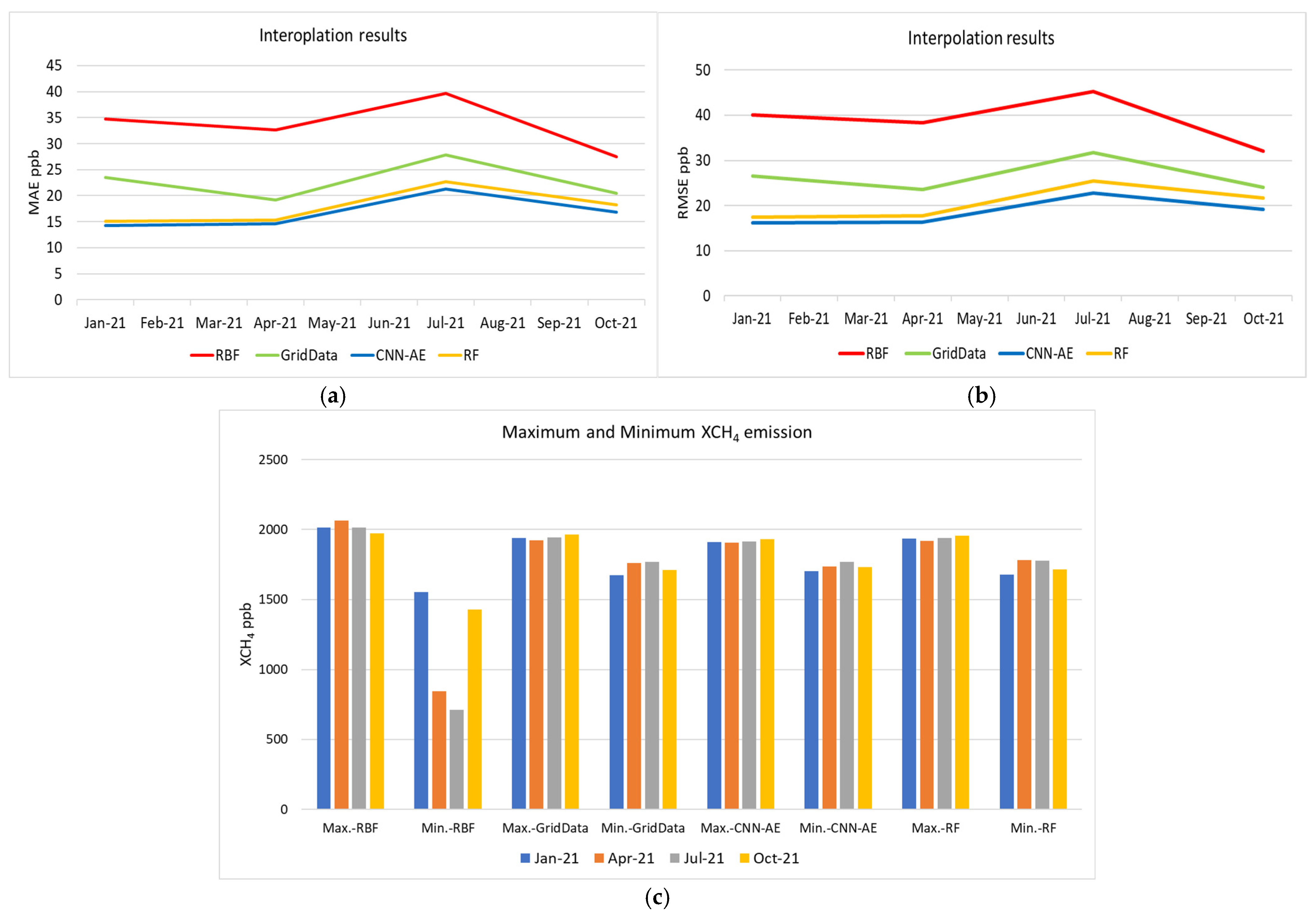
Verifying the Predicted and Interpolated Values

The verification of the results provided by different methods was based on the selected TCCON stations for the years 2019 and 2021. Several methods were used to verify the results, which can be summarized as follows:

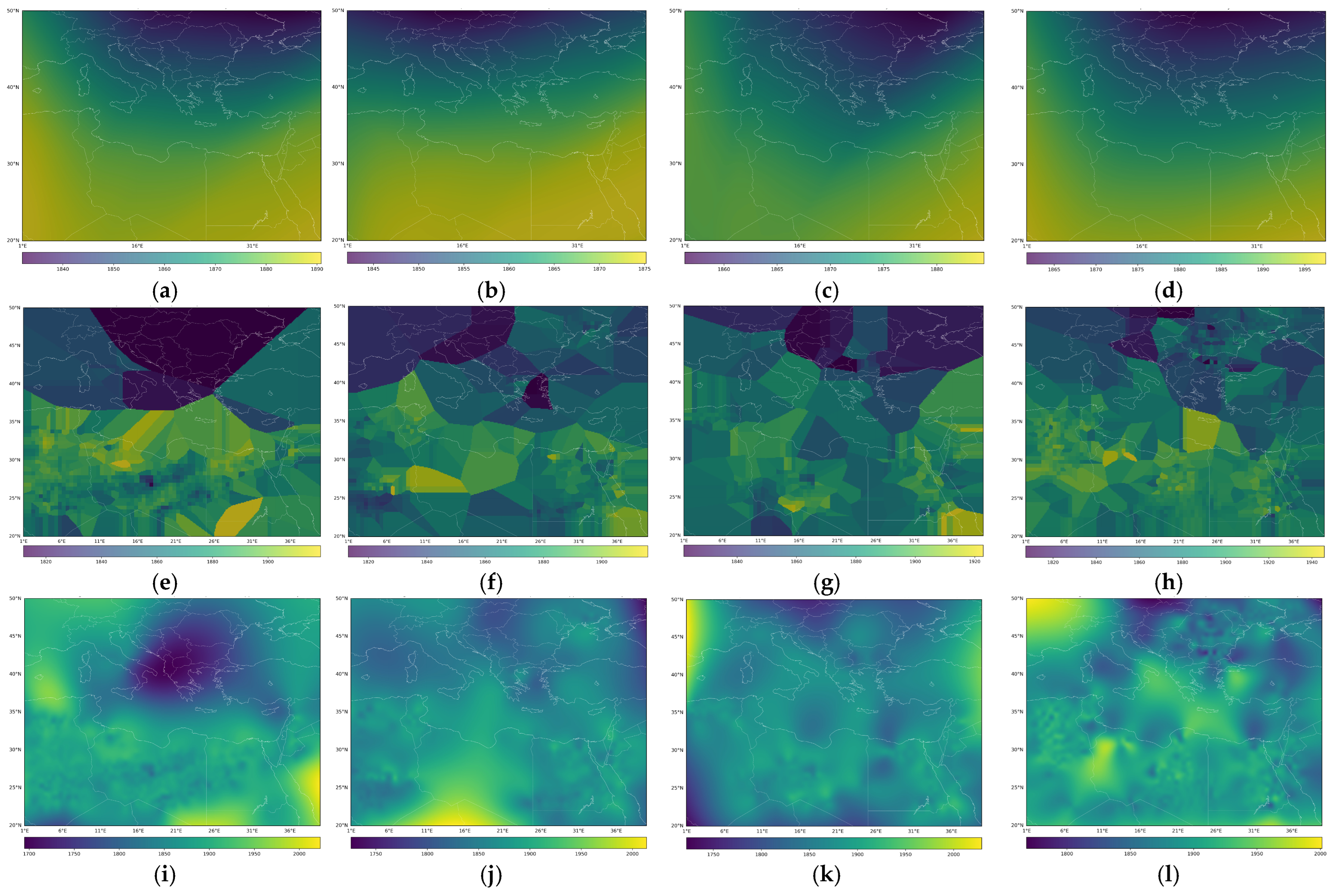
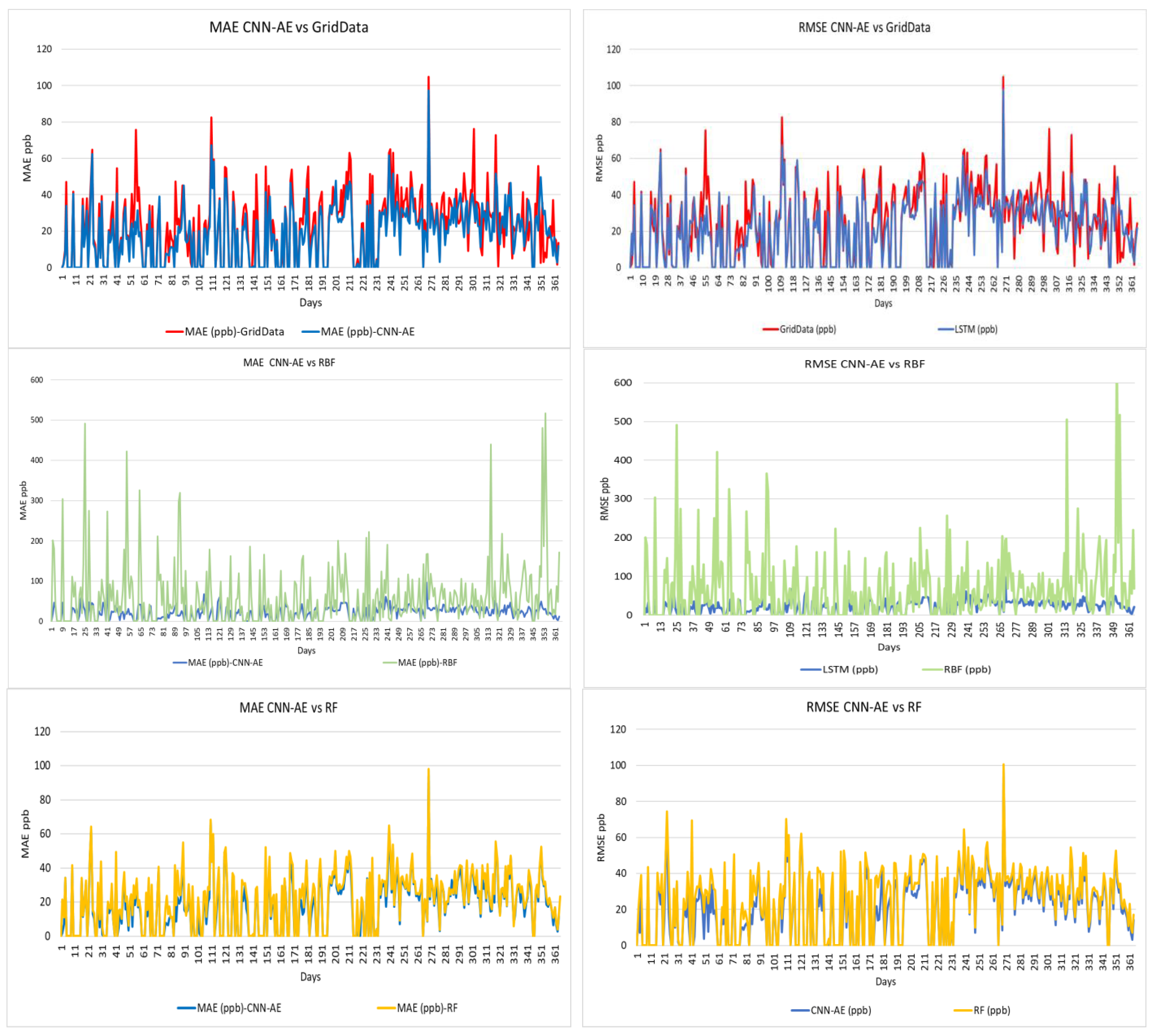
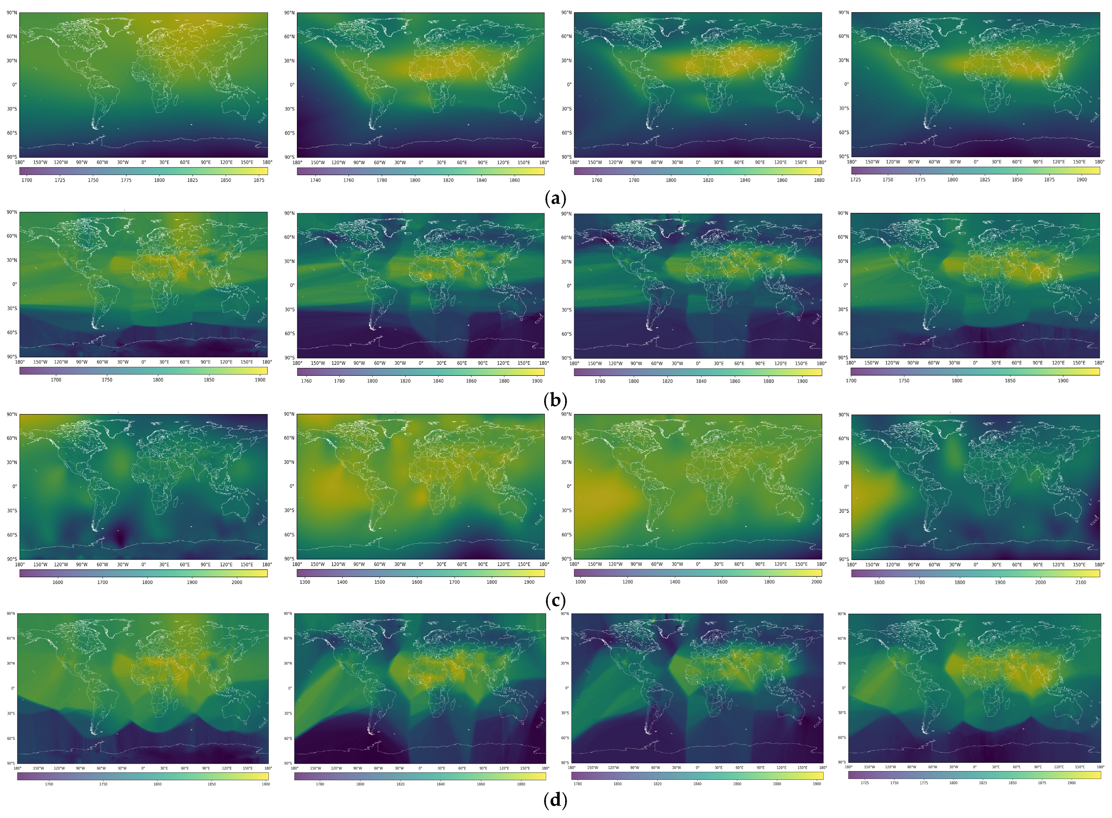
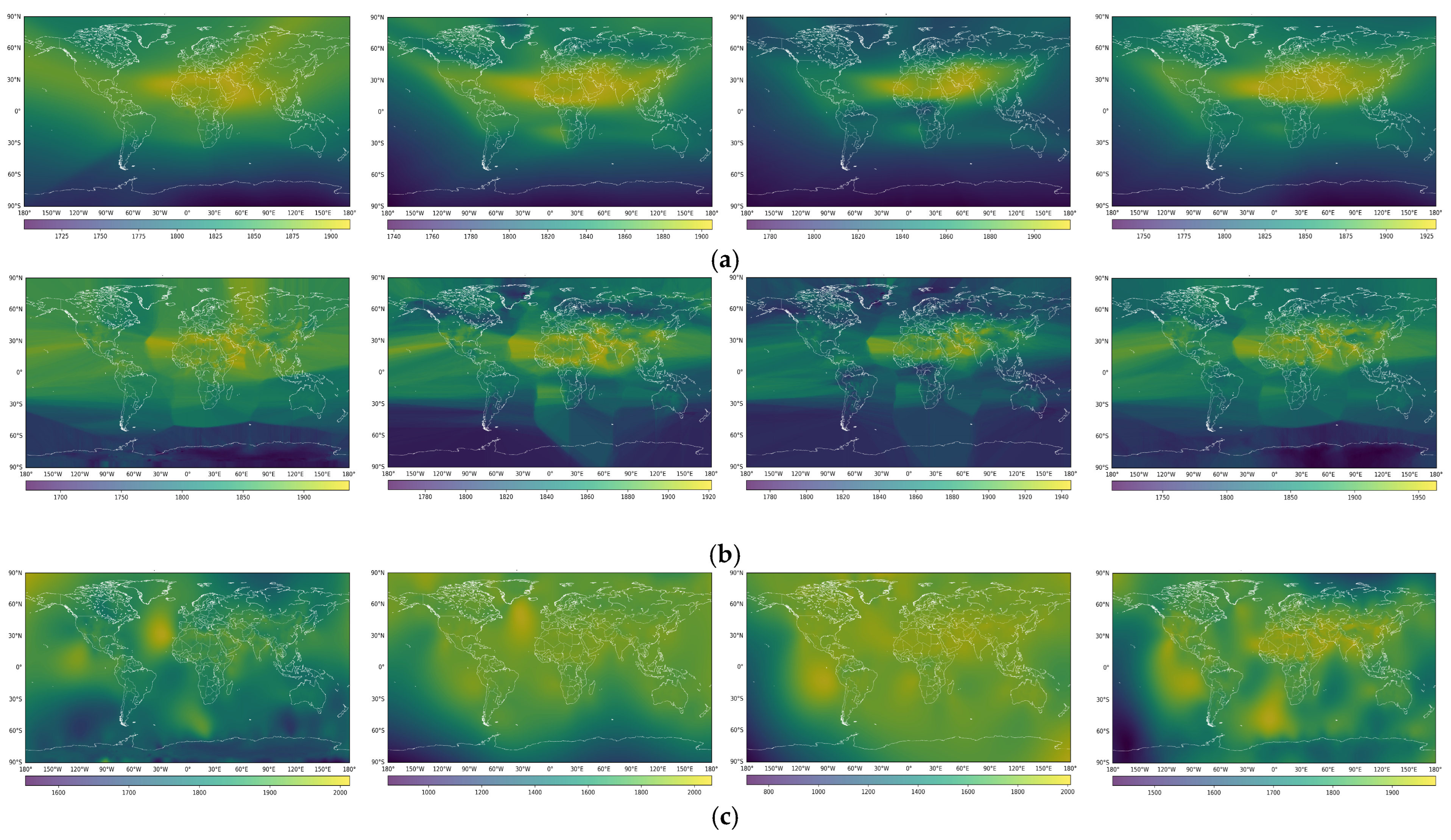
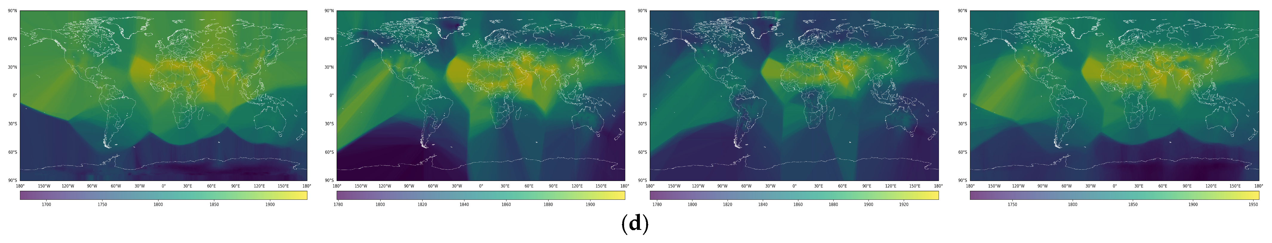
• Visual Comparison: Plotting the predicted, interpolated, and observed values on graphs to inspect how well the predictions match the observations visually.
• Statistical Comparison: Calculating statistical measures to quantify the differences between predicted/interpolated and observed values. Common metrics include

Mean Absolute Error (MAE) [30]: The average of the absolute differences between predicted and observed values.

$$MAE=\frac{1}{N}{\sum }_{i=1}^N\left|\widehat{y_i}-y_i\right|$$

(12)

where N is the number of observations, $\widehat{y_i}$ is the predicted value, and $y_i$ is the observed value. MAE < 1 ppm indicates that, on average, the model’s predictions are within 1 ppm of the actual XCH₄ values.

Also, the Root Mean Square Error (RMSE) [32] was used in this research for several reasons: 1. Penalizes large errors more than MAE: RMSE squares the differences between predicted and actual values, giving higher weight to larger errors. 2. Maintains the same units as the target variable: Unlike MSE (Mean Squared Error), which results in squared units, RMSE retains the original units of the predicted variable, making it easier to interpret in practical applications. 3. Works well in normally distributed errors: For datasets where errors follow a Gaussian distribution, RMSE is more effective than MAE at capturing overall error magnitude. The following Equation calculates the RMSE:

$$RMSE=\sqrt[2]{\frac{1}{N}{\sum }_{i=1}^N{(\widehat{y_i}-y_i)}^2}$$

(13)

3. Results

The experiments covered one complete year, 2019, and four different months in all seasons from 2019 and 2021. The decision to use the identified periods (January, April, July, and October 2019 to 2021) was based on the seasonal variations in XCH₄ levels in the northern hemisphere. Fluctuations in methane levels are driven by a combination of human activities and natural processes. In spring (April and May), methane levels often peak due to increased emissions from wetlands as temperatures rise, combined with agricultural activities like rice planting and livestock farming. In summer (June and July), methane levels tend to decrease as higher temperatures and increased vegetation enhance the breakdown of methane in the atmosphere through chemical reactions. In autumn (October and November), another peak can occur due to reduced vegetation cover and increased emissions from sources like biomass burning and fossil fuel use for heating. Finally, in winter (December–February), XCH₄ concentrations in the northern hemisphere tend to rise or stabilize due to a combination of anthropogenic and natural factors.

Figure 5a–d show the result of running our new method (CNN-AE). Figure 5e–h show the outcome of running SciPy GridData NNI to estimate and create XCH₄ for specific dates. Figure 5i–l show the result of running the Radial Basis Function (RBF) Interpolator for the same data collected on the same date as the previous interpolation technique. Finally, Figure 5m–p show the result of running Random Forest (RF).

Please note that the resolution of the generated grids or mesh is 0.1 degrees due to the extensive volume of data utilized to estimate the global XCH₄ levels. It is visually evident from the figures that RF, NNI, and RBF performance are the worst due to significant inconsistencies and discontinuities between different areas of the predicted data. On the contrary, CNN-AE looks more homogeneous, smooth, continuous, and consistent. To prove the efficiency of CNN-AE in predicting data, the MAE and RMSE were calculated based on the available XCH₄ data emission provided by TCCON stations. CNN-AE had the lowest MAE and RMSE values of 28.48 and 30.07 ppb, followed by RF regressor 29.07 and 36.89 ppb, NNI 30.06 and 32.14 ppb, and finally RBF 80.23 and 90.54 ppb. Moreover, comparing the results with those of the Sentinel-5p TROPOMI displayed in the maps of Figure 1, it is clear that the south and the east of the Mediterranean basin have the highest concentration of XCH₄. Additionally, the generated XCH₄ values by RF, RBF, and NNI exhibit random and inconsistent patterns. In contrast, CNN-AE provides continuous data, clearly showing that XCH₄ levels are higher in the south area of the Mediterranean than in the north. MAE and RMSE were computed for all the results obtained by different interpolation models for all available data during the year 2019. All MAE and RMSE values are displayed in Figure 6 to show the efficiency of CNN-AE, yielding the lowest error values between the predicted and actual values obtained from TCCON stations. One can also notice in the graph that some MAE and RMSE values are zero due to the absence of TCCON data. Moreover, it is noticeable that high peaks of MAE errors belong to RF, NNI, and RBF methods.

In the second experiment, the global area (world) was selected with data that covers four different seasons in two different years, 2019 and 2021. Figure 7 shows the result of running different interpolation models. These images show the average XCH₄ in different months (January, April, July, and October) that represent different seasons in 2019.

To demonstrate the efficiency of the CNN-AE model in comparison to SciPy’s GridData (NNI), RBF, and RF methods, the results were validated against TCCON station data, using MAE and RMSE as evaluation metrics. Figure 8a illustrates the MAE values computed for all three techniques across various months in 2019, highlighting their relative accuracy over time. As one can see, the new model, CNN-AE, achieved the lowest MAE compared to RF, NNI, and RBF. Figure 8b shows the computed RMSE; again, CNN-AE has the lowest value compared to the other models. Moreover, Figure 8c shows the maximum and minimum of the XCH₄, which helps in understanding which model works more efficiently than the others. One can notice that RBF has large differences between the minimum and maximum XCH₄ emission, which explains why MAE and RMSE are higher compared to the other three methods of interpolation.

A third experiment was conducted on data that covers four different months in 2021, similar to the previous experiment. The experiment helped in understanding the changes in XCH₄ during two different periods. Figure 9 shows the results of running different interpolation models.

Again, the TCCON stations’ data were used to validate the obtained results (Figure 10a,b). Moreover, the maximum and minimum emissions of XCH₄ predicted by the different interpolation models were shown on a graph (Figure 10b). One can notice again that after comparing the different evaluation metrics (MAE and RMSE), it appeared that CNN-AE is the best model compared to RF, GridData (NNI), and RBF, respectively. The averages of MAE and RMSE for the two years were computed for all models. The CNN-AE model demonstrated superior performance, achieving the lowest MAE and RMSE of 19.78 and 24.7 ppb, followed by RF with 21.46 and 27.23 ppb, GridData (NNI) with 25.3 and 32.62 ppb, and RBF with 43.08 and 54.93 ppb.

Based on the data provided by the CNN-AE model, which includes both maximum and minimum emissions of column-averaged methane (XCH₄), a clear upward trend in methane concentrations can be observed. Specifically, the minimum recorded XCH₄ levels increased from 1723.5 ppb in 2019 to 1734.25 ppb in 2021, indicating a measurable rise in baseline atmospheric methane.

Furthermore, the maximum XCH₄ emissions also exhibited a notable increase, rising from 1888.75 ppb in 2019 to 1916 ppb in 2021. This upward shift in both the lower and upper bounds of methane concentration suggests a persistent rise in atmospheric methane levels over the study period, which may have implications for greenhouse gas monitoring and climate change mitigation strategies. Before industrialization, atmospheric XCH₄ was estimated to be around 720 ppb. This value is derived from ice core records and historical atmospheric reconstructions [33].

4. Discussion

In this research, a new Autoencoder CNN (CNN-AE) was created to predict the XCH₄ missing values and fill the gaps inherent in the available satellites, such as Sentinel-5P TROPOMI. The new model, CNN-AE, overcame many obstacles, preventing available interpolation models published in the literature from predicting XCH₄ values daily and for both small and large areas. The work of Jiang et al. [9] used a combination of DINEOF and the Bayesian Maximum Entropy (BME) to compensate for missing data every month. However, CNN-AE was able to fill in missing data daily, even with a limited number of XCH₄ points.

Wefers et al.’s methodology XCH₄SAT+ [11] used data from multiple satellite missions, combining them through statistical interpolation techniques to enhance temporal and spatial coverage. In contrast, CNN-AE used one source of data, Sentinel-5p, and provided more reliable results. In comparing the CNN-AE model with the XGBoost-based retrieval approach proposed by Zhang et al. [17], several key advantages emerge that highlight the superior performance of CNN-AE in methane concentration estimation. While Zhang et al. utilized XGBoost to extract XCH₄ values from Sentinel-5P TROPOMI data, the method primarily focused on feature selection and efficient retrieval rather than optimizing spatial and temporal continuity. Their TRO_XGB_XCH₄ model achieved a ground-based validation R of 0.749 and a temporal extension accuracy R of 0.863, demonstrating respectable agreement with official satellite products but without explicit evaluation of mean errors or spatial interpolation accuracy. In contrast, the CNN-AE hybrid approach demonstrated marked improvements in retrieval precision, particularly at both regional and global scales. The new model achieved an MAE and RMSE of 28.48 and 30.07 ppb, followed by RF Regressor with 29.07 and 36.89 ppb, GridData NNI with 30.06 and 32.14 ppb, and RBF with 80.23 and 90.54 ppb. For global XCH₄ reconstruction, CNN-AE continued to show superior accuracy, with the lowest MAE and RMSE of 19.78 and 24.7 ppb, followed by RF with 21.46 and 27.23 ppb, GridData NNI with 25.3 and 32.62 ppb, and RBF with 43.08 and 54.93 ppb.

This clear advantage underscores the effectiveness of deep learning hybrid approaches in enhancing data reconstruction and spatial coherence, which is a crucial factor in atmospheric monitoring. Unlike XGBoost, CNN-AE inherently captures nonlinear temporal dependencies through sequential learning, which aids in refining methane concentration estimates more reliably over time. Additionally, its interpolation capability ensures improved data continuity, making it an excellent tool for satellite-based environmental studies. Thus, while XGBoost provides a computationally efficient alternative for methane retrieval, CNN-AE demonstrates superior accuracy, enhanced spatial–temporal consistency, and reduced error margins, positioning it as a more robust methodology for methane monitoring applications.

5. Conclusions

This study presents the development and application of a hybrid CNN-AE model for predicting daily XCH₄ concentrations over both large and small regions, utilizing satellite data from methane monitoring missions such as Sentinel-5P TROPOMI. The model demonstrates superior accuracy, spatial coverage, and temporal consistency compared to traditional interpolation methods, including GridData and Radial Basis Function (RBF) Interpolator.

Key findings from this approach include the following:

Enhanced Data Consistency: The CNN-AE model produces homogeneous and reliable XCH₄ predictions, effectively capturing seasonal variations in atmospheric methane. It aligns well with observed trends, reflecting higher methane levels in regions with intensified emissions.

Addressing Data Gaps: Traditional interpolation models often struggle with irregularly distributed satellite observations, leading to discontinuities in methane mapping. The CNN-AE model significantly reduces data gaps, ensuring comprehensive spatial coverage and improving overall dataset reliability.

Scalability and Adaptability: The model’s architecture allows for flexible deployment across different spatial and temporal resolutions, making it well-suited for methane monitoring at both regional and global scales. Additionally, its design enables the integration of additional remote sensing data for further refinement.

By delivering daily high-resolution XCH₄ estimates, this new model outperforms traditional methods in methane data reconstruction and environmental monitoring applications. Its ability to enhance spatial continuity and retrieval accuracy represents a significant advancement in atmospheric science, contributing to improved methane tracking for climate research, greenhouse gas mitigation, and policy-making. Future efforts will focus on further optimizing the CNN-AE model, extending its application to other atmospheric constituents, incorporating hyperspectral imaging sources, and integrating real-time monitoring systems for enhanced global methane cycle analysis.

References

1. Schneising, O.; Buchwitz, M.; Reuter, M.; Heymann, J.; Bovensmann, H.; Burrows, J.P. Long-term analysis of carbon dioxide and methane column-averaged mole fractions retrieved from SCIAMACHY. Atmos. Chem. Phys. 2011, 11, 2863–2880. [Google Scholar] [CrossRef]
2. Reuter, M.; Buchwitz, M.; Schneising, O.; Noel, S.; Bovensmann, H.; Burrows, J.P.; Boesch, H.; Di Noia, A.; Anand, J.; Parker, R.J.; et al. Ensemble-based satellite-derived carbon dioxide and methane column-averaged dry-air mole fraction data sets (2003–2018) for carbon and climate applications. Atmos. Meas. Tech. 2020, 13, 789–819. [Google Scholar] [CrossRef]
3. Saunois, M.; Stavert, A.R.; Poulter, B.; Bousquet, P.; Canadell, J.G.; Jackson, R.B.; Raymond, P.A.; Dlugokencky, E.J.; Houweling, S.; Patra, P.K.; et al. The Global Methane Budget 2000–2017. Earth Syst. Sci. Data 2020, 12, 1561–1623. [Google Scholar] [CrossRef]
4. Solomon, S. Climate Change 2013: The Physical Science Basis. Working Group 1 Contribution to the IPCC Fifth Assessment Report; Cambridge University Press: Cambridge, UK, 2013. [Google Scholar]
5. European Space Agency (ESA), Sentinel-5P Tropomi. Available online: https://www.esa.int/Applications/Observing_the_Earth/Copernicus/Sentinel-5P (accessed on 21 April 2025).
6. Kuze, A.; Suto, H.; Nakajima, M.; Hamazaki, T. Thermal and near infrared sensor for carbon observation Fourier-transform spectrometer on the Greenhouse Gases Observing Satellite for greenhouse gases monitoring. Appl. Opt. 2009, 48, 6716–6733. [Google Scholar] [CrossRef] [PubMed]
7. Suto, H.; Kuze, A.; Shiomi, K.; Nakajima, M. Recent progress of GOSAT series for greenhouse gas monitoring. Remote Sens. 2021, 13, 689. [Google Scholar] [CrossRef]
8. McLinden, C.A.; Griffin, D.; Davis, Z.; Hempel, C.; Smith, J.; Sioris, C.; Nassar, R.; Moeini, O.; Legault-Ouellet, E.; Malo, A. An Independent Evaluation of GHGSat Methane Emissions: Performance Assessment. J. Geophys. Res. Atmos. 2024, 129, e2023JD039906. [Google Scholar] [CrossRef]
9. Jiang, Y.; Gao, Z.; He, J.; Wu, J.; Christakos, G. Application and Analysis of XCO2 Data from OCO Satellite Using a Synthetic DINEOF–BME Spatiotemporal Interpolation Framework. Remote Sens. 2022, 14, 4422. [Google Scholar] [CrossRef]
10. Azcarate, A.A.; Barth, A.; Sirjacobs, D.; Lenartz, F.; Beckers, J.M. Data Interpolating Empirical Orthogonal Functions (DINEOF): A tool for geophysical data analyses. Mediterr. Mar. Sci. 2011, 12, 5–11. [Google Scholar] [CrossRef]
11. Wefers, W.; Lehnert, L.; Schmidt, D.; Reuter, M.; Buchwitz, M.; Kammann, C.; Velten, K.; Hase, F.; Notholt, J.; Kubistin, D.; et al. Approximation of multi-year time series of XCO2 concentrations using satellite observations and statistical interpolation methods. Atmos. Res. 2023, 294, 106965. [Google Scholar] [CrossRef]
12. Hu, K.; Zhang, Q.; Feng, X.; Liu, Z.; Shao, P.; Xia, M.; Ye, X. An Interpolation and Prediction Algorithm for XCO2 Based on Multi-Source Time Series Data. Remote Sens. 2024, 16, 1907. [Google Scholar] [CrossRef]
13. Liu, H.; Zhang, Y.; Chen, Y. A Symmetric Efficient Spatial and Channel Attention (ESCA) Module Based on Convolutional Neural Networks. Symmetry 2024, 16, 952. [Google Scholar] [CrossRef]
14. Hochreiter, S.; Schmidhuber, J. Long short-term memory. Neural Comput. 1997, 9, 1735–1780. [Google Scholar] [CrossRef] [PubMed]
15. Sheng, M.; Lei, L.; Zeng, Z.C.; Rao, W.; Song, H.; Wu, C. Global land 1° mapping dataset of XCO2 from satellite observations of GOSAT and OCO-2 from 2009 to 2020. Big Earth Data 2022, 7, 170–190. [Google Scholar] [CrossRef]
16. Zeng, Z.-C.; Lei, L.; Strong, K.; Jones, D.B.A.; Guo, L.; Liu, M.; Lin, H. Global land mapping of satellite-observed CO2 total columns using spatio-temporal geostatistics. Int. J. Digit. Earth 2016, 10, 426–456. [Google Scholar] [CrossRef]
17. Zhang, W.; Li, Y.; Li, B.; Li, T.; Wang, Z.; Yang, X.; Jin, Y.; Zhang, L. Retrieval of Atmospheric XCH4 via XGBoost Method Based on TROPOMI Satellite Data. Atmosphere 2025, 16, 279. [Google Scholar] [CrossRef]
18. Mueller, J.P.; Massaron, L. Python for Data Science for Dummies; John Wiley & Sons: Hoboken, NJ, USA, 2015; p. 432. [Google Scholar]
19. Cardille, J.A.; Crowley, M.A.; Saah, D.; Clinton, N.E. (Eds.) Cloud-Based Remote Sensing with Google Earth Engine: Fundamentals and Applications; Springer: Cham, Switzerland, 2024; p. 1226. [Google Scholar] [CrossRef]
20. Lorente, A.; Borsdorff, T.; Butz, A.; Hasekamp, O.; de Brugh, J.A.; Schneider, A.; Wu, L.; Hase, F.; Kivi, R.; Wunch, D.; et al. Methane retrieved from TROPOMI: Improvement of the data product and validation of the first 2 years of measurements. Atmos. Meas. Tech. 2021, 14, 665–684. [Google Scholar] [CrossRef]
21. Rocha, H. On the selection of the most adequate radial basis function. Appl. Math. Model. 2009, 33, 1573–1583. [Google Scholar] [CrossRef]
22. Lazzaro, D.; Montefusco, L. Radial basis functions for the multivariate interpolation of large scattered data sets. J. Comput. Appl. Math. 2002, 140, 521–536. [Google Scholar] [CrossRef]
23. Winkel, B.; Lenz, D.; Flöer, L. Cygrid, A fast Cython-powered convolution-based gridding module for Python. Astron. Astrophys. 2016, 591, A12. [Google Scholar] [CrossRef]
24. Liaw, A.; Wiener, M. Classification and Regression by randomForest. R News 2002, 2, 18–22. [Google Scholar]
25. Ioffe, S.; Szegedy, C. Batch normalization: Accelerating deep network training by reducing internal covariate shift. In Proceedings of the 32nd International Conference on Machine Learning (ICML), Lille, France, 6–11 July 2015; Volume 37, pp. 448–456. [Google Scholar] [CrossRef]
26. Glorot, X.; Bordes, A.; Bengio, Y. Deep sparse rectifier neural networks. In Proceedings of the Fourteenth International Conference on Artificial Intelligence and Statistics (AISTATS), Fort Lauderdale, FL, USA, 11–13 April 2011; Volume 15, pp. 315–323. [Google Scholar]
27. Srivastava, N.; Hinton, G.; Krizhevsky, A.; Sutskever, I.; Salakhutdinov, R. Dropout: A simple way to prevent neural networks from overfitting. J. Mach. Learn. Res. 2014, 15, 1929–1958. [Google Scholar]
28. Huber, P.J. Robust estimation of a location parameter. Ann. Math. Stat. 1964, 35, 73–101. [Google Scholar] [CrossRef]
29. Benesty, J.; Chen, J.; Huang, Y.; Cohen, I. Mean squared error: A powerful performance measure for speech enhancement. In Noise Reduction in Speech Processing; Springer: Berlin/Heidelberg, Germany, 2009; Volume 2, pp. 1–40. [Google Scholar] [CrossRef]
30. Chai, T.; Draxler, R.R. Root mean square error (RMSE) or Mean absolute error (MAE)?—Arguments against avoiding RMSE in the literature. Geosci. Model Dev. 2014, 7, 1247–1250. [Google Scholar] [CrossRef]
31. Kingma, D.P.; Ba, J. Adam: A method for stochastic optimization. In Proceedings of the 3rd International Conference on Learning Representations (ICLR), Banff, AB, Canada, 14–16 April 2014. [Google Scholar] [CrossRef]
32. Hodson, T.O. Root-mean-square error (RMSE) or mean absolute error (MAE): When to use them or not. Geosci. Model Dev. 2022, 15, 5481–5487. [Google Scholar] [CrossRef]
33. Copernicus Climate Change Service. Climate Data Store. Methane data from 2002 to Present Derived from Satellite Observations. Copernicus Climate Change Service (C3S) Climate Data Store (CDS). 2018. Available online: https://doi.org/10.24381/cds.b25419f8 (accessed on 14 June 2025).
Figure 1. Global XCH4 abundance in different seasons of 2019 (Sentinel-5P).
Atmosphere 16 00806 g001
Figure 2. TCCON stations in the (a) global area, (b) regional area.
Atmosphere 16 00806 g002
Figure 3. The processes to estimate and map XCH4.
Atmosphere 16 00806 g003
Figure 4. CNN-AE model (a) general structure, (b) encoder, (c) decoder.
Atmosphere 16 00806 g004
Figure 5. Examples of XCH4 for different days in the year 2019 (Days 26, 118, 198, and 290) predicted by (ad) CNN-AE, (eh) NNI, (il) RBF, (mp) RF Regressor.
Atmosphere 16 00806 g005aAtmosphere 16 00806 g005b
Figure 6. Verification of the different methods for the first study area (year 2019).
Atmosphere 16 00806 g006
Figure 7. Monthly average of XCH4 for 4 different months in 2019 (January, April, July, and October) created by (a) CNN-AE, (b) NNI, (c) RBF, (d) RF.
Atmosphere 16 00806 g007
Figure 8. Year 2019: (a,b) The results of validation of XCH4 interpolation using MAE and RMSE; (c) minimum and maximum of XCH4 by different interpolation models in different months.
Atmosphere 16 00806 g008
Figure 9. Monthly average of XCH4 for 4 different months in 2021 created by (a) CNN-AE, (b) NNI, (c) RBF, (d) RF.
Atmosphere 16 00806 g009aAtmosphere 16 00806 g009b
Figure 10. Year 2021: (a,b) The results of validation of XCH4 interpolation using MAE and RMSE; (c) minimum and maximum of XCH4 by different interpolation models in different months.
Atmosphere 16 00806 g010