A Signal Processing-Guided Deep Learning Framework for Wind Shear Prediction on Airport Runways

Abstract

Wind shear at the Hong Kong International Airport (HKIA) poses a significant safety risk due to terrain-induced airflow disruptions near the runways. Accurate assessment is essential for safeguarding aircraft during take-off and landing, as abrupt changes in wind speed or direction can compromise flight stability. This study introduces a hybrid framework for short-term wind shear prediction based on data collected from Doppler LiDAR systems positioned near the central and south runways of the HKIA. These systems provide high-resolution measurements of wind shear magnitude along critical flight paths. To predict wind shear more effectively, the proposed framework integrates a signal processing technique with a deep learning strategy. It begins with optimized variational mode decomposition (OVMD), which decomposes the wind shear time series into intrinsic mode functions (IMFs), each capturing distinct temporal characteristics. These IMFs are then modeled using bidirectional gated recurrent units (BiGRU), with hyperparameters optimized via the Tree-structured Parzen Estimator (TPE). To further enhance prediction accuracy, residual errors are corrected using Extreme Gradient Boosting (XGBoost), which captures discrepancies between the reconstructed signal and actual observations. The resulting OVMD–BiGRU–XGBoost framework exhibits strong predictive performance on testing data, achieving R² values of 0.729 and 0.926, RMSE values of 0.931 and 0.709, and MAE values of 0.624 and 0.521 for the central and south runways, respectively. Compared with GRUs, LSTM, BiLSTM, and ResNet-based baselines, the proposed framework achieves higher accuracy and a more effective representation of multi-scale temporal dynamics. It contributes to improving short-term wind shear prediction and supports operational planning and safety management in airport environments.

1. Introduction

1.1. Wind Shear: Hidden Dangers

Wind shear is a transient phenomenon that changes over time and is influenced by dynamic atmospheric conditions [1,2]. It refers to a rapid change in wind speed or direction over a short distance, occurring horizontally or vertically, and is often associated with sharp temperature inversions or atmospheric density gradients. According to the International Civil Aviation Organization (ICAO), wind shear is defined as a change in wind speed and/or direction in space, including updrafts and downdrafts [3]. This broad definition encompasses a variety of meteorological phenomena, such as thunderstorms, frontal systems, and low-level jet streams, all of which can produce hazardous conditions for aircraft, particularly during takeoff and landing. The Federal Aviation Authority (FAA) publication P-8740-40 identifies four principal sources of wind shear, including frontal shear, convective activity, temperature inversions, and surface-induced effects [4]. Frontal wind shear becomes likely when the temperature contrast across a front exceeds 10 °F (5 °C) and the frontal boundary advances at speeds above 30 knots. Convective sources such as thunderstorms introduce severe shear through phenomena like first gusts and downbursts. Gusts may reach 100 knots and shift direction by up to 180°, while downbursts exhibit vertical velocities surpassing 720 feet per minute at low altitudes, compromising aircraft performance. Temperature inversion shear develops when nocturnal cooling forms a stable layer near the surface, interacting with faster-moving air above and often causing abrupt directional shifts and wind speed surges at the ground level. Surface obstructions such as buildings or terrain features disrupt airflow patterns and generate localized shear, particularly under strong wind conditions near the surface.

1.2. Impact of Wind Shear on Aircraft

Wind shear poses a serious risk to aircraft, especially during takeoff and landing, when the aircraft is close to the ground and has limited room to recover from sudden changes [2]. Sharp shifts in wind speed or direction can upset lift and air speed, making it harder for pilots to keep the aircraft stable. To manage this risk, aviation relies on accurate and timely weather forecasts. When wind shear is detected in advance, pilots can adjust their flight plans, change speeds, or delay departures and arrivals to stay out of danger. Air traffic controllers also benefit from this information, as it helps them guide aircraft more safely through busy airspace. With the support of modern forecasting tools and real-time weather data, aviation crews can spot signs of wind shear earlier and take action before it becomes a problem [5]. This preparation helps prevent accidents, keeps flights on schedule, and improves safety for everyone on board.

1.3. Wind Shear Detection Technologies

The application of advanced remote sensing technologies such as Terminal Doppler Weather Radar (TDWR) and Doppler Light Detection and Ranging (LiDAR) across numerous international airports has led to substantial improvements in the detection of wind shear. These technologies operate alongside ground-based anemometer networks and wind profilers to create a comprehensive monitoring system. Since the mid-1990s, these methods have helped airports identify and respond to dangerous wind conditions, especially during tropical cyclones and severe convective weather. TDWR has served as a key tool for identifying wind shear near airports [6,7]. However, its performance can drop in clear-sky conditions because it relies on moisture in the air to reflect radar signals. In situations where there is little or no precipitation, the system may struggle to detect changes in wind. To improve coverage, airports have turned to Doppler LiDAR as a helpful addition [8,9]. Unlike radar, LiDAR picks up signals from tiny particles in the air, such as dust or aerosols, which remain even when skies are clear. This makes it possible to measure wind patterns more accurately when traditional radar falls short.

By combining both systems, airports can track wind shear in a wider variety of weather conditions and give pilots and controllers more useful information to help them respond safely during flight operations. While the operational benefits of these systems are well established, their deployment and maintenance involve several challenges. High acquisition and installation costs, the need for continuous system calibration, and the requirement for skilled technical personnel represent significant barriers. Smaller airports may struggle to justify the investment due to limited budgets and lower traffic volumes. Moreover, integrating these technologies into existing infrastructure can prove logistically complex. Despite these constraints, the enhanced precision and reliability in detecting wind shear continue to make these systems valuable assets in the pursuit of safer and more efficient aviation operations [10,11,12].

1.4. Wind Shear Forecasting

While modern systems like TDWR and Doppler LiDAR can detect wind shear near airports, they cannot predict the precise timing or cause of future events. Reliable forecasting remains a key challenge in maintaining flight safety, particularly during takeoff and landing when aircraft are most vulnerable to sudden wind shifts. Without timely forecasts, crews may receive alerts too late to respond effectively. Accurate predictions allow pilots and controllers to make informed adjustments before conditions deteriorate. Recent studies point to the growing potential of artificial intelligence (AI) in improving wind shear forecasting. One such study employed a combination of principal component analysis (PCA) and k-means clustering to assess the impact of turbulence on aircraft performance [13]. Similarly, to assess the severity of wind shear, the BalanceCascade framework combined with SHAP has been used to enhance the classification of severe wind shear (S-WS) and non-severe (NS-WS) events [14]. In a separate approach, conditional generative adversarial networks (CGANs) were integrated with XGBoost to analyze turbulence based on LiDAR data, revealing complex atmospheric structures with greater clarity [15]. In a real-time identification of hazardous thunderstorm conditions, the random forest (RF) model played a key role in detecting aviation turbulence [16].

Moreover, some researchers applied a hybrid model that combines a support vector machine (SVM) and deep neural network (DNN) to assess the likelihood of flight incident risks based on operational data in the domain of aviation safety [17]. To predict the aircraft system failures, multi-layer perceptron (MLP) models in conjunction with support vector regression (SVR) have been employed [18]. Some researchers assessed anomalies and failures in aircraft onboard systems by using recurrent neural networks (RNNs) [19]. In addition, flight delays, airport operations, and aircraft missed approaches were also estimated using AI frameworks, such as the application of the attention-based bidirectional long short-term memory (AB-LSTM) approach to improve the prediction of flight delays [20], deep neural networks (DNNs) that supported airport-level forecasts of departure delays [21], and using the long short-term memory (LSTM) model to estimate boarding duration [22]. Similarly, wind shear-induced missed approaches were estimated by using an Explainable Boosting Machine (EBM) [23]. Feature importance analysis revealed that wind shear altitude was the most influential factor contributing to the occurrence of missed approaches. Similarly, pairwise interaction analysis illustrated the combination of precipitation and wind shear magnitude had the highest joint impact on missed approaches

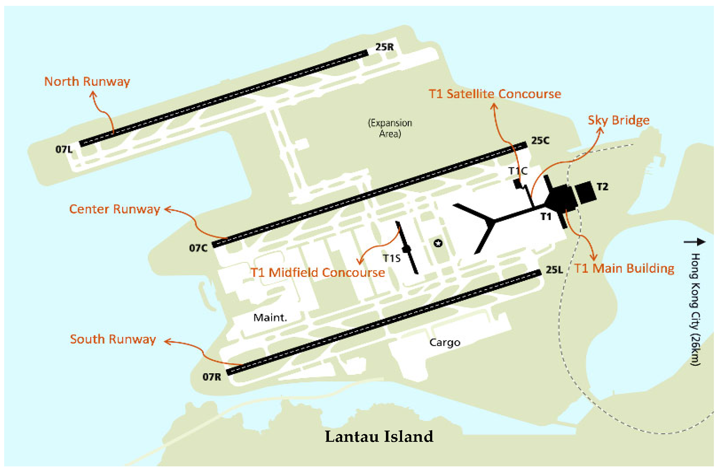
1.5. Hong Kong International Airport as Wind Shear-Prone Airport

Hong Kong International Airport (HKIA) is the primary aviation hub for Hong Kong, located on the northeastern edge of Lantau Island. The site was developed through large-scale land reclamation along the subtropical coastline of southern China, as shown in Figure 1. Its location near major commercial centers in the Asia–Pacific region gives it a strategic advantage in international air traffic flow [24]. It is equipped with advanced infrastructure and a well-planned layout. The HKIA ranks among the world’s top airports for both passenger traffic and cargo volume. Hong Kong International Airport operates three parallel runways designated 07L/25R, 07C/25C, and 07R/25L, oriented approximately east to west. This configuration supports independent parallel operations, allowing simultaneous takeoffs and landings during standard conditions and contributing to increased airfield capacity. Runway 07R/25L, located on the southern edge of the airfield, lies closest to the passenger terminals and cargo facilities. Its position shortens taxi distances and facilitates efficient movement of both passenger and freight aircraft. The central runway, 07C/25C, was originally designated 07L/25R. It was renamed in December 2021 after the addition of the third runway to reflect its central position within the layout. This runway was temporarily closed for reconfiguration and resurfacing and resumed operations on 28 November 2024. Runway 07L/25R, situated on the northern side of the airport, is the newest of the three and was developed as part of the Three-Runway System (3RS) project.

Although the HKIA features a modern infrastructure, it often faces hazardous weather events. The nearby terrain, including the hills of Lantau Island to the south, influences wind behavior around the airport. Wind shear continues to pose a serious risk, with observed magnitudes between 14 and 30 knots [25,26]. Around 75% of wind shear events documented through Pilot Reports (PIREPs) at the HKIA are associated with strong downslope winds from the surrounding terrain, often driven by tropical cyclones or intense monsoon flows. Sea breeze interactions account for approximately 15% of wind shear occurrences at the HKIA. The remaining 10% are linked to factors such as low-level jets, gust fronts, microbursts, or turbulence influenced by the airport’s built environment [27].

Figure 1. Aerial layout of HKIA (source: [28]).

Figure 1. Aerial layout of HKIA (source: [28]).

1.6. Research Contribution

To address the irregular, non-stationary, and complex characteristics of wind shear events, this study presents a hybrid signal processing-guided deep learning framework. The structure integrates signal decomposition, sequential modeling, probabilistic optimization, and machine learning refinement, aiming to improve forecasting accuracy at the HKIA. The contributions are as follows:

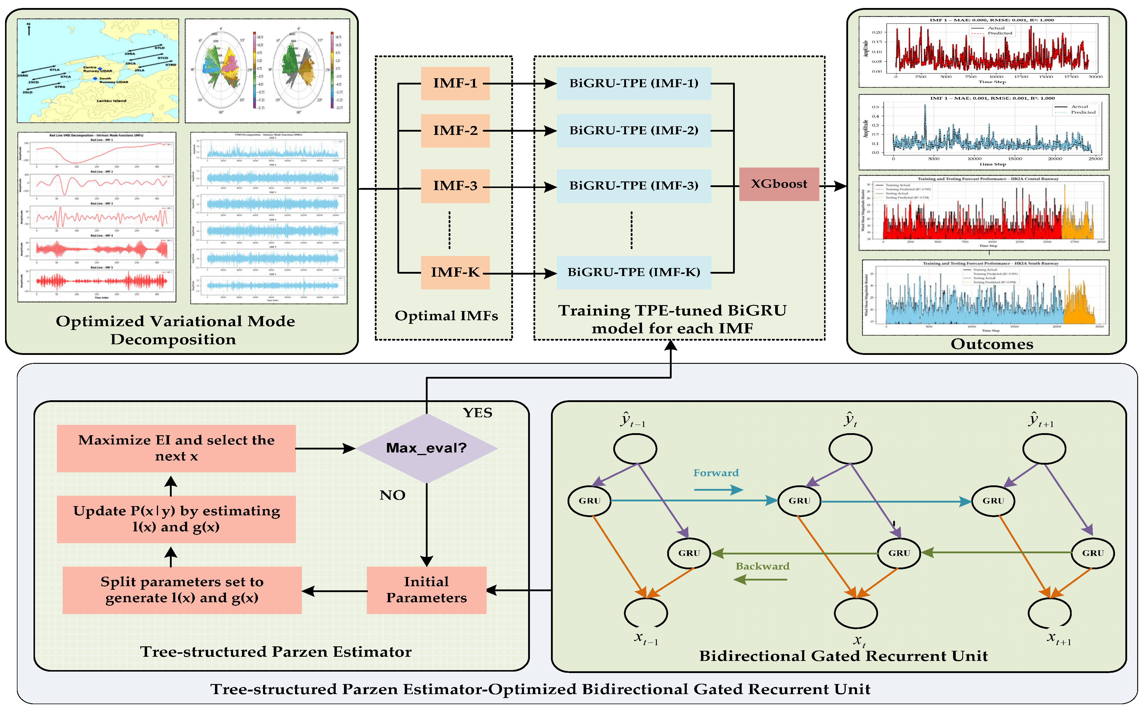
• Wind shear data recorded at the HKIA often displays abrupt changes and multi-scale variability influenced by terrain-induced disturbances. To address these characteristics, the study applies optimized variational mode decomposition (OVMD) to divide the original time series into intrinsic mode functions (IMFs), with each IMF representing a specific frequency component [29,30]. This decomposition enhances temporal resolution, reduces noise interference, and exposes features that are essential for modeling wind shear behavior more precisely.
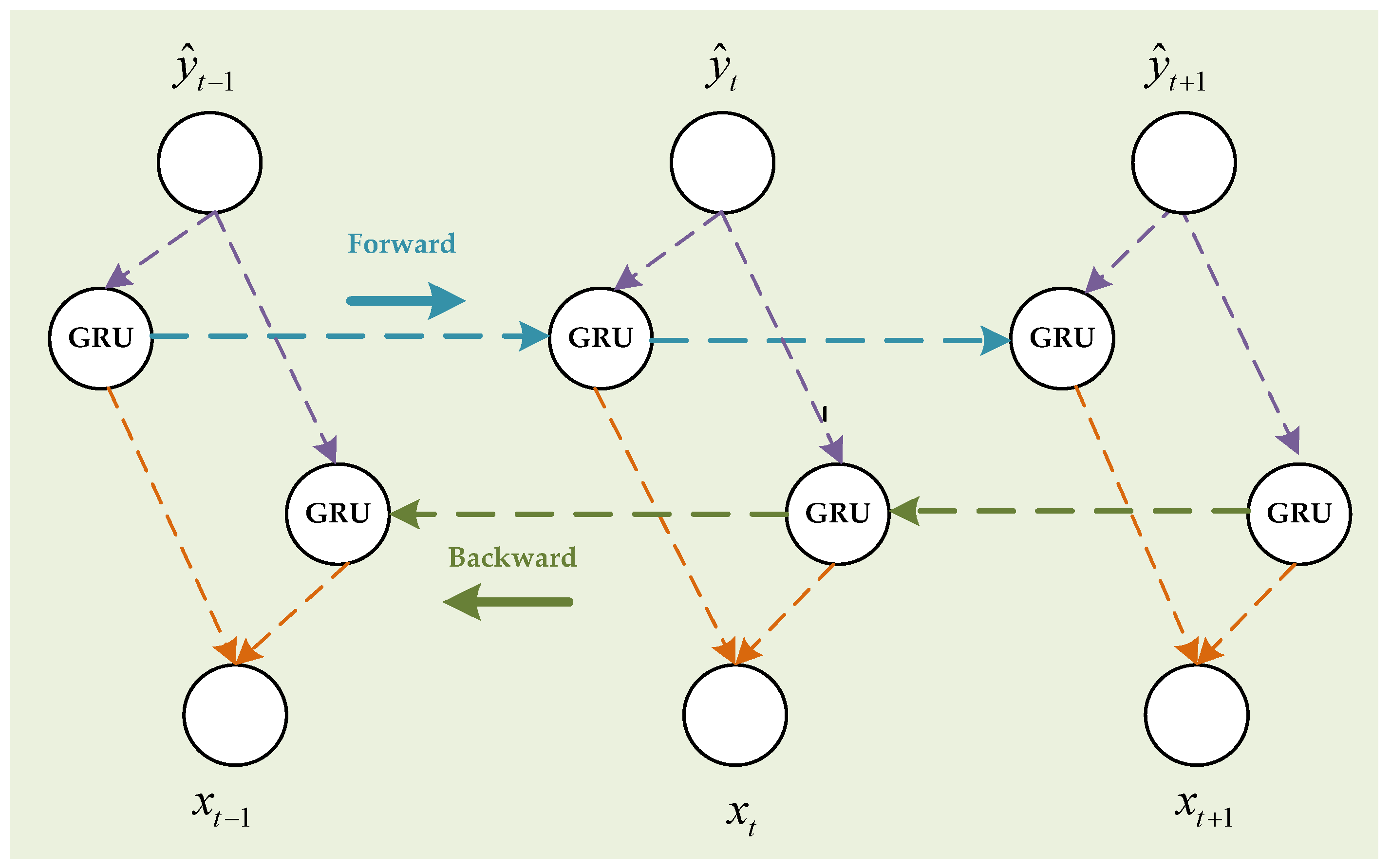
• Each IMF is modeled independently using a bidirectional gated recurrent unit (BiGRU) network [22,31,32]. This structure captures temporal dependencies in both forward and backward directions and adapts to the evolving nature of the underlying patterns across different IMFs. Hyperparameters for BiGRUs are selected through the Tree-structured Parzen Estimator (TPE) [33,34] to maintain balance between generalization and responsiveness to localized fluctuations in the data.
• Residual prediction errors from the BiGRU stage are further refined using an Extreme Gradient Boosting (XGBoost) model [35]. This stage identifies non-linear deviations and remaining signal components that are not captured by the deep learning stage. XGBoost improves overall prediction accuracy by correcting these discrepancies, which often reflect the irregular and abrupt nature of wind shear near airport runways.

Figure 2 presents the signal processing-guided deep learning framework developed for wind shear prediction. The rest of the paper is structured as follows: Section 2 describes the study area, introduces the Doppler LiDAR data collected at the HKIA, and provides a theoretical overview of the signal processing-guided deep learning framework for the assessment of wind shear along with the evaluation metrics. Section 3 discusses the analysis of the results and assesses model performance. Section 4 concludes the study by summarizing key findings and providing directions for future work.

2. Materials and Methods

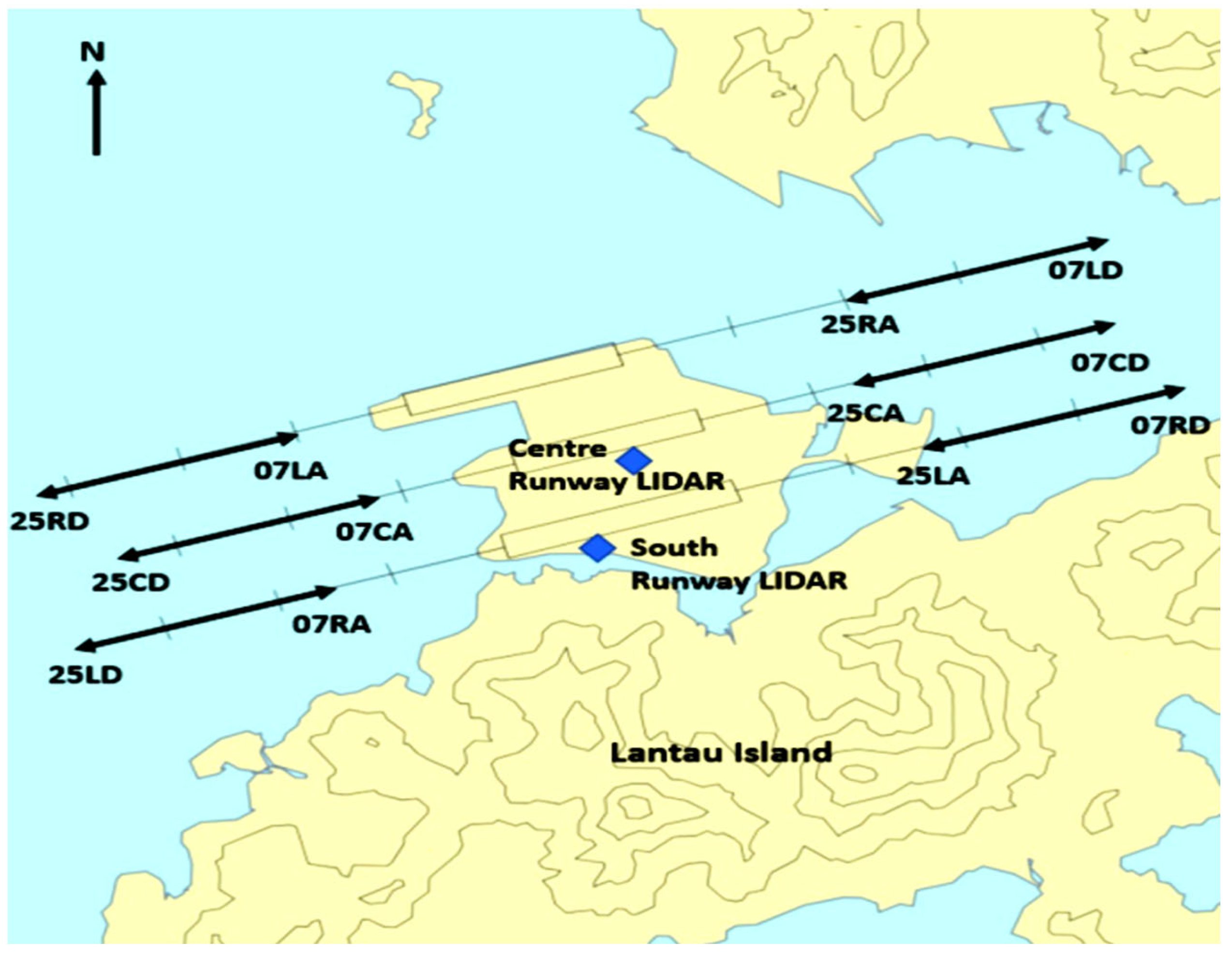
2.1. HKIA Doppler LiDAR System

The Doppler LiDAR system at the HKIA serves as a core instrument for wind shear detection and analysis. The first unit was installed on the rooftop of the air traffic control complex in August 2002 to obtain direct observation of the approach and departure runways. A second identical unit was added in 2006 to extend spatial coverage and increase data reliability. This installation represented the first operational use of Doppler LiDAR technology worldwide for aviation weather alerts. The system operates at wavelengths of 1.5 and 2 μm and emits high-frequency laser pulses to trace aerosol movement and determine radial wind velocity. With a range resolution of approximately 100 m, it captures wind speeds up to 40 m/s under extended configurations. The north LiDAR targets the operational modes of the north runway, while the south unit focuses on the central and south runways, as illustrated in Figure 3.

Two scanning strategies support wind shear detection, namely fixed-elevation plan position indicator (PPI) scans and glide path scans (GPScans). The GPScan method, developed by the Hong Kong Observatory, directs the laser beam along three-degree glide paths from the runway thresholds to construct headwind profiles. The scanner operates within an azimuth range of 220° to 280° at a fixed elevation angle of 3°, covering slant distances between 350 and 4950 m. PPI scans provide wind velocity fields at high spatial and temporal resolution, where negative velocity values represent wind directed toward the LiDAR and positive values indicate wind directed away. These measurements help delineate headwind and tailwind zones across flight corridors. Based on the radial velocity data, the GLYGA algorithm detects wind shear by locating sharp transitions in headwind across specific ramp lengths. It calculates a severity factor by combining the headwind increment with the inverse cube root of ramp length. When this factor exceeds the operational threshold of 14 knots, the system triggers an alert. The dual-LiDAR configuration at the HKIA ensures continuous and precise monitoring of wind shear conditions, particularly under dry weather.

Figure 4 shows the radial wind velocity in knots, as recorded by the Doppler LiDAR at the HKIA. The system uses the PPI mode at a 3° elevation angle and scans slant ranges between 350 m and 10,000 m. Warm colors such as yellow, orange, pink, and brown represent positive velocities, where wind moves away from the LiDAR. Cool colors such as green, blue, and purple indicate negative velocities, where wind moves toward the LiDAR. Each PPI scan consists of 400 to 500 laser beams and takes about 20 to 30 s to complete. Blank sectors at longer slant ranges reflect areas where the surrounding terrain blocks the line of sight of the LiDAR, leading to missing data.

Table 1. Data instances obtained from the Doppler LiDAR covering the central runway.

Date and Time	Wind Shear Magnitude (Knots)	Elevation Angle (°)	Azimuth Angle (°)	Assigned Runway	Encounter Location
29 January 2017 18:36	30	(3.00 3.00)	(221, 271.5)	25CA	2 MF
15 March 2018 15:41	24	(3.00 3.00)	(278, 260.5)	07CA	1 MF
-	-	-	-	-	-
27 January 2019 7:02	16	(3.00 3.00)	(265, 242.5)	07CD	RWY
-	-	-	-	-	-
11 June 2020 21:08	24	(3.00 3.00)	(225, 230.5)	25CA	RWY
15 October 2021 15:41	21	(3.00 3.00)	(278, 260.5)	07CA	1 MD

and

Table 2. Data instances obtained from the Doppler LiDAR covering the south runway.

Date and Time	Wind Shear Magnitude (Knots)	Elevation Angle (°)	Azimuth Angle (°)	Assigned Runway	Encounter Location
27 May 2017 5:37	23	(3.00 3.00)	(223, 248.5)	07LA	1 MD
18 August 2019 18:42	35	(3.00 3.00)	(262, 276.3)	25LA	1 MF
-	-	-	-	-	-
11 March 2020 16:55	18	(3.00 3.00)	(249, 273.5)	25LA	2 MD
-	-	-	-	-	-
20 August 2021 11:03	30	(3.00 3.00)	(280, 220.5)	07RD	RWY
18 October 2021 5:31	20	(3.00 3.00)	(262, 269.5)	07RA	2 MF

present sample instances of wind shear events recorded by Doppler LiDAR systems at the HKIA between 2017 and 2022 for the central and southern runways, respectively. The central runway is designated as such in this study, although it was previously referred to as the north runway prior to the commissioning of the new north runway after 2022. Data for the new north runway is not yet available and is therefore not included in this analysis. Each entry includes the date and time, wind shear magnitude (knots), fixed elevation angle of 3.00°, azimuth angle, assigned runway, and encounter location. The data represents two operational zones, including the former north runway, now redesignated as the central runway (07C/25C), and the south runway (07R/25L). Runway identifiers such as 07CA, 07CD, 25CA, 07RA, 07RD, and 25LA specify the operational direction and flight phase during each event. Encounter locations including 1MD, 1MF, 2MD, 2MF, and RWY denote positions relative to the runway. For example, “1MF” denotes a location within 0–1 nautical miles on final approach (MF: miles at final) from the threshold of the runway. A wind shear event labeled as “1MF” for runway 07R occurs within the first nautical mile on approach to that runway. In contrast, “1MD” represents a location within 0–1 nautical miles after departure (MD: miles at departure) from the end of the runway. For instance, “1MD” on runway 25L indicates an event detected within the first nautical mile after takeoff. Similarly, “2MF” and “2MD” refer to locations 1–2 nautical miles on final approach and after departure, respectively. The glide path on approach remains fixed at 3 degrees, while the departure angle varies with aircraft type and takeoff weight.

2.2. Hybrid OVMD–GRU–XGBoost Framework for Time Series Analysis

The wind shear magnitude time series displays irregular patterns without a clear trend or recurring structure, making short-term forecasting more challenging. Sudden fluctuations between consecutive observations further complicate the modeling of temporal dependencies. This study presents a hybrid forecasting framework that integrates OVMD, BiGRU networks, and a residual correction mechanism based on XGBoost, with hyperparameter tuning performed using TPE. The process starts with OVMD, which decomposes the original wind shear time series into a set of IMFs, each representing distinct frequency characteristics of the signal. This decomposition enhances data quality by isolating localized temporal features and reducing noise. Each IMF is then modeled using a BiGRU network to capture temporal dependencies in both forward and backward directions. TPE is employed to optimize the hyperparameters of each BiGRU model for improved performance. Next, the residuals between the aggregated BiGRU predictions and the actual wind shear values are modeled using an XGBoost regression model, capturing remaining non-linear patterns not learned by the BiGRU models. This residual learning step serves as a final correction to the forecast, enhancing overall accuracy. The segmentation logic and architecture of the proposed hybrid framework are detailed in the following section.

2.2.1. Optimized Variational Mode Decomposition (OVMD)

The first stage of the proposed hybrid framework functions as a signal preprocessing step, where the original wind shear time series is decomposed into a finite set of IMFs, each corresponding to a specific frequency band. This decomposition improves feature separability, mitigates noise, and enhances the model’s ability to capture intrinsic temporal structures. OVMD is employed to break down the real-valued signal $x(t)$ into K band-limited modes ${\left\{u_k(t)\right\}}_{k=1}^K$, each centered around an adaptively estimated frequency ${\omega }_k$. This process is formulated as a constrained variational problem, as presented in Equation (1).

$$\underset{\left\{{\mu }_k\right\},\left\{{\omega }_k\right\}}{\min }\left\{{\displaystyle \sum _{k=1}^k{‖{\partial }_t\left[\left(\delta \left(t\right)+\frac{j}{\pi t}\right)\ast {\mu }_k\left(t\right)\right]e^{-{j\omega }_{k}t}‖}_2^2}\right\}s.t. {\displaystyle \sum _{k=1}^k{\mu }_k\left(t\right)=x\left(t\right)}$$

(1)

To address this constrained variational problem, an augmented Lagrangian formulation is adopted, as shown in Equation (2). This reformulation transforms the original optimization task into a more tractable form by decomposing it into sub-problems that are easier to handle computationally. This approach allows efficient numerical implementation of the OVMD process.

$$\begin{array}{l}\varpi \left(\left\{{\mu }_k\right\},\left\{{\omega }_k\right\},\lambda \right)= \alpha {\displaystyle \sum _{k=1}^k{‖{\partial }_t\left[\left(\delta \left(t\right)+\frac{j}{\pi t}\right)\ast {\mu }_k\left(t\right)\right]e^{-{j\omega }_{k}t}‖}_2^2}+{‖x\left(t\right)-{\displaystyle \sum _{k=1}^k{\mu }_k\left(t\right)}‖}_2^2 \\ +〈\lambda \left(t\right),x\left(t\right)-{\displaystyle \sum _{k=1}^k{\mu }_k\left(t\right)}〉\end{array}$$

(2)

where $\alpha$ is the quadratic penalty factor, $\lambda \left(t\right)$ is the Lagrange multiplier, $\ast$ denotes convolution, $\delta \left(t\right)$ is the Dirac delta function, and $j$ is the imaginary unit.

It is important to note that the performance of VMD is highly sensitive to the selection of two critical parameters, i.e., the number of decomposition modes K and the penalty factor $\alpha$. To determine the optimal number of IMFs K, Fast Fourier Transform (FFT) is performed on the original signal to identify distinct frequency bands [38]. Each peak in the frequency domain corresponds to a potential IMF, and the number of such significant peaks is selected as the optimal K. The penalty factor $\alpha$ controls the trade-off between mode bandwidth compactness and data reconstruction, and its optimization is conducted through mutual information analysis [39]. Let $x(t)$ be the original signal and $IM{F}_i\left(t\right)$ the $i^{th}$ decomposed component. The maximum MI across IMFs is given by Equation (3).

$${MI}_{\alpha }^{\max }=\max \left(MI\left({x,IMF}_1\right),MI\left({x,IMF}_2\right),\dots ,MI\left({x,IMF}_k\right)\right)$$

(3)

Equation (3) determines the most informative IMF relative to the original signal. It quantifies the degree to which each decomposed component retains essential characteristics $x(t)$ of the original time series, ensuring that the decomposition remains meaningful and is not excessively diffuse or noise-driven. The reconstructed signal $x^{\prime }\left(t\right)$ is obtained by summing all extracted IMFs, as expressed in Equation (4). This reconstructed signal is then compared to the original series to assess how effectively the decomposition preserves the structural and energetic properties of the input signal.

$$x\prime \left(t\right)={\displaystyle \sum _{i=1}^{K}IM{F}_i}\left(t\right)$$

(4)

The variable ${\beta }_{\alpha }$ is obtained and measures the global similarity between the original signal and its reconstruction, as illustrated in Equation (5). A higher value implies better fidelity of the reconstructed signal and less information loss during decomposition.

$${\beta }_{\alpha }=MI\left(x\left(t\right),x\prime \left(t\right)\right)$$

(5)

The overall evaluation metric ${\gamma }_{\alpha }$ is computed, which integrates both local and global aspects of the decomposition, retaining the most informative component and ensuring the overall signal integrity, as shown by Equation (6). This balanced criterion allows the framework to select an $\alpha$ that avoids both mode mixing and under-decomposition.

$${\gamma }_{\alpha }={\beta }_{\alpha }\cdot M{I}_{\alpha }^{\max }$$

(6)

Then, the optimal penalty factor ${\alpha }^{\ast }$ is determined by maximizing the evaluation metric ${\gamma }_{\alpha }$, which is shown by Equation (7).

$${\alpha }^{\ast }=\arg \underset{a}{max}{ \gamma }_{\alpha }$$

(7)

With the optimized values $K^{\ast }$ and ${\alpha }^{\ast }$, the final decomposition of the wind shear magnitude time series is expressed as Equation (8):

$$x\left(t\right)={\displaystyle \sum _{i=1}^{K^{\ast }}IM{F}_i}\left(t\right)={\displaystyle \sum _{i=1}^{K^{\ast }}{A}_i\left(t\right)}\cos \left({\varphi }_i\left(t\right)\right)$$

(8)

where $A_i\left(t\right)$ is the amplitude envelope of the $i^{th}$ IMF and ${\varphi }_i\left(t\right)$ is the instantaneous phase.

2.2.2. BiGRU Component Optimized via TPE

Once the wind shear magnitude time series $x(t)$ is decomposed into $K^{\ast }$ IMFs through OVMD, each $IM{F}_i\left(t\right)$ captures distinct frequency characteristics of the original signal. These components are generally smoother and exhibit improved stationarity, making them more appropriate for sequence learning models. Each $IM{F}_i\left(t\right)$ is modeled individually using the BiGRU network to forecast its future values. The BiGRU is a sequence learning architecture that processes data in both forward and backward directions, enabling it to capture long-term dependencies and extract temporal features more effectively than a unidirectional GRU model.

Let the input sequence for the $i^{th}$ IMF be $X^{\left(i\right)}=\left\{x_1^{\left(i\right)},x_2^{\left(i\right)},\dots ,x_T^{\left(i\right)}\right\}$, where the goal is to generate the predicted sequence ${\widehat{Y}}^{\left(i\right)}=\left\{{\widehat{y}}_1^{\left(i\right)},{\widehat{y}}_2^{\left(i\right)},\dots ,{\widehat{y}}_T^{\left(i\right)}\right\}$, approximating the ground truth values ${\widehat{Y}}^{\left(i\right)}$. At each time step $t$, the BiGRU processes the input from both temporal directions, as shown in Figure 5. The forward hidden state for the $i^{th}$ IMF is computed as Equation (9) and simultaneously, the backward hidden state is derived by Equation (10).

$${\overrightarrow{h}}_t^{(t)}=GR{U}_{fwd}\left(x_t^{(i)},{\overrightarrow{h}}_{t-1}^{(t)}\right)$$

(9)

$${\overleftarrow{h}}_t^{(t)}=GR{U}_{bwd}\left(x_t^{(i)},{\overleftarrow{h}}_{t+1}^{(t)}\right)$$

(10)

Then, the forward and backward hidden states produced by the BiGRU are concatenated to form a comprehensive bidirectional representation, as shown in Equation (11). This combined representation integrates information from both past and future contexts within the sequence, enhancing the model’s ability to capture complex temporal dynamics in the wind shear signal.

$$\stackrel{ (t)}{h_t}=\left[{\overrightarrow{h}}_t^{(t)};{\overleftarrow{h}}_t^{(t)}\right]$$

(11)

The output prediction at each time step is generated by feeding the corresponding hidden state into a fully connected (dense) layer, as expressed in Equation (12). This transformation maps the learned bidirectional temporal features to the final forecasted value for the wind shear magnitude.

$${\widehat{y}}_t^{\left(i\right)}=W_0{h}_t^{(i)}+b_0$$

(12)

Here, $W_0\in {\Re }^{1\times 2h}$ and $b_0\in {\Re }^{1\times 2h}$ represent the learnable parameters of the output layer.

The model is trained by minimizing the mean squared error (MSE) between the actual and predicted values of each IMF, as defined in Equation (13). This loss function allows each decomposed sub-series to contribute independently to the overall learning process, allowing for tailored adjustments during optimization and improving the ability of model to capture the unique dynamics of each component.

$${\tau }^{\left(i\right)}={\displaystyle \frac{1}{T}}{{\displaystyle \sum _{t=1}^T\left(y_t^{(i)}-{\widehat{y}}_t^{(i)}\right)}}^2$$

(13)

To achieve optimal predictive performance for each IMF component, the BiGRU models are individually fine-tuned using the TPE, which is basically a Bayesian optimization technique that efficiently explores the hyperparameter space [40]. For the BiGRU model trained on the $i^{th}$ IMF, let the set of hyperparameters subject to optimization be denoted as Equation (14).

$${\theta }^{\left(i\right)}=\left\{u,\eta ,d,b\right\}$$

(14)

where ${\theta }^{\left(i\right)}\in \Theta$ represents a candidate configuration from the hyperparameter search space $\Theta$. $u$ denotes the number of hidden units, $\eta$ is the learning rate, $d$ represents the dropout rate, and $b$ is the batch size.

The objective is to identify the optimal set ${\theta }^{\left(i\right)\ast }$ that minimizes the validation loss ${\tau }^{\left(i\right)}$, defined earlier in Equation (13), for the corresponding IMF. This optimization problem can be expressed as Equation (15).

$${\theta }^{\left(i\right)\ast }=\arg \underset{{\theta }^{\left(i\right)}\in \Theta }{\min }{\tau }^{\left(i\right)}\left({\theta }^{\left(i\right)}\right)$$

(15)

The TPE algorithm models the objective function ${\tau }^{\left(i\right)}$ as a probabilistic process by constructing two density estimators, i.e., $p\left(\theta |\tau \right)$ is the conditional probability of hyperparameter configurations given observed losses and $p\left(\tau \right)$ is the marginal probability over observed loss values. The TPE divides observed hyperparameter–loss pairs into two groups, as shown by Equations (16) and (17).

$${\mathcal{D}}_{good}=\left\{\theta |\tau \left(\theta \right)\le {\tau }^{\ast }\right\}$$

(16)

$${\mathcal{D}}_{bad}=\left\{\theta |\tau \left(\theta \right)>{\tau }^{\ast }\right\}$$

(17)

where ${\tau }^{\ast }$ is a quantile threshold (typically the 10–25th percentile of losses). The algorithm then models the distributions $l\left(\theta \right)=p\left(\theta |\tau \le {\tau }^{\ast }\right)$ and $g\left(\theta \right)=p\left(\theta |\tau >{\tau }^{\ast }\right)$ and samples new candidates that maximize the expected improvement criterion, as shown by Equation (18).

$$EI\left(\theta \right)\propto {\displaystyle \frac{l\left(\theta \right)}{g\left(\theta \right)}}$$

(18)

This strategy enhances the probability that new trials are sampled from promising regions of the search space, which accelerates convergence and lowers the risk of becoming stuck in local minima. By applying TPE to optimize the hyperparameters of each IMF-specific BiGRU, the framework aligns more effectively with the temporal complexity of individual components. This results in improved predictive accuracy and greater stability in the final aggregated forecast.

2.2.3. Reconstruction and Residual Correction

After each $IM{F}_i$ is modeled and predicted using its individually optimized BiGRU model, the final step involves aggregating the predicted values to reconstruct the fine forecasted wind shear time series signal. Let ${\widehat{y}}_t^{\left(i\right)}$ denote the predicted value at time $t$ for the $IM{F}_i$ component. The reconstructed signal ${\widehat{y}}_t$, representing the predicted wind shear magnitude at time ${\widehat{y}}_t^{\left(i\right)}$, is computed as the sum of all predicted IMFs, as shown in Equation (19).

$${\widehat{y}}_t={\displaystyle \sum _{i=1}^K{\widehat{y}}_t^{\left(i\right)}}$$

(19)

However, this naive summation may introduce cumulative errors. To refine the final prediction, a residual correction is applied using XGBoost, a gradient-boosted decision tree ensemble. Let the residual be defined as Equation (20).

$$e_t=y_t-{\widehat{y}}_t$$

(20)

Each $e_t$ is modeled using XGBoost with the IMF-level GRU predictions $\begin{array}{l}\left[{\widehat{y}}_t^{\left(1\right)}\dots ,{\widehat{y}}_t^{(K)}\right]\\ \end{array}$ as input features. The XGBoost learner fits a series of weak regressors $f_m\left(.\right)\in F$, minimizing Equation (21).

$${\psi }_{xgb}={\displaystyle \sum _{t=1}^{T}l\left(e_t,{\widehat{e}}_t\right)}+{\displaystyle \sum _{m=1}^M\Phi \left(f_m\right)}$$

(21)

where $l$ represents the squared error loss $\begin{array}{l}l\left(e_t,{\widehat{e}}_t\right)={\left(e-\widehat{e}\right)}^2\\ \end{array}$ and $\Phi \left(f\right)=\gamma T+{\displaystyle \frac{1}{2}}\lambda {‖\omega ‖}^2$ is the regularization term with number of leaves T and weights $\omega$.

The corrected final forecast is then computed as Equation (22).

$${\widehat{y}}_{t,final}={\widehat{y}}_t+{\widehat{e}}_t$$

(22)

2.3. Performance Metrics

To evaluate the predictive performance of the proposed VMD–GRU–XGBoost model and compare it against several benchmark models, a set of standard error metrics is employed. These include the mean squared error (MSE), root mean squared error (RMSE), and the coefficient of determination (R²). The MSE and RMSE measure the average magnitude of forecast errors, with the RMSE providing results in the same units as the original data, making interpretation more intuitive. In contrast, R² quantifies the proportion of variance in the observed data explained by the model, reflecting overall model fit. A comprehensive summary of these evaluation criteria, including their definitions and mathematical expressions, is presented in

Table 3. Description of performance metrics.

Metric	Description	Expression
MSE	Calculates the mean of the squared deviations between the predicted and actual values.	${\displaystyle \frac{1}{N}}{{\displaystyle {\sum }_{x=1}^N\left(y_x-{\overline{y}}_x\right)}}^2$
RMSE	Represents the square root of the mean squared differences between predicted outputs and actual observations.	$\sqrt{{\displaystyle {\sum }_{x=1}^N\frac{{\left(y_x-y_x\right)}^2}{N}}}$
R2	Indicates the proportion of variance in the actual values that is explained by the model’s predictions, reflecting how well the model fits the observed data.	$1-{\displaystyle \frac{{\displaystyle \sum _{x=1}^N{\left(y_x-{\widehat{y}}_x\right)}^2}}{{\displaystyle \sum _{x=1}^N{\left(y_x-{\overline{y}}_x\right)}^2}}}$

.

3. Results and Discussion

The Doppler LiDAR dataset from the Hong Kong International Airport (HKIA) contains wind shear measurements collected between 1 January 2017 and 31 December 2021. These observations correspond to aircraft operations on the central and south runways. The directional segments include 07CA, 07CD, 25CA, and 25CD for the central runway and 07RA, 07RD, 25LA, and 25LD for the south runway. A total of 128,344 data points were recorded for the central runway and 163,177 for the south runway, capturing wind shear behavior across critical operational paths.

To develop and validate the model, the data was divided using an 85 to 15 ratio. The first portion, comprising 109,092 samples from the central runway and 138,700 samples from the south runway, was used for training and hyperparameter tuning. This allowed the model to learn the underlying temporal characteristics of wind shear. The remaining 19,252 samples for the central runway and 24,477 samples for the south runway were reserved for testing. They are shown as time series in Figure 6a,b. The data split followed the natural time sequence of the observations. This arrangement provided a clear separation between the periods used for learning and those used for evaluation, allowing the performance to be assessed on data that had not influenced the training process.

Figure 7a,b presents the probability distribution of wind shear magnitudes for the central and south runways, respectively, using histograms with kernel density estimates (KDEs). Most wind shear magnitudes fall between 14 and 18 knots, forming positively skewed distributions. The south runway shows a broader spread and higher frequency of extreme values, indicating greater variability in wind behavior near this zone.

Figure 7c,d illustrates the monthly distribution of wind shear magnitudes across the two runways using violin plots. The central runway displays consistent distributional patterns throughout the year, with stable medians and compact interquartile ranges. In contrast, the south runway exhibits higher variability and a slight upward shift in median magnitudes between July and September, potentially influenced by seasonal factors such as convective activity or thermal gradients near the southern approach paths. Figure 7e,f depicts hourly trends in average wind shear magnitude along with one standard deviation envelopes. Both runways show limited diurnal variation, though a slight bimodal structure is observable, particularly at the central runway. The south runway reveals higher overall mean values and broader variability in the late afternoon and evening hours, which may relate to localized effects including terrain-induced turbulence or boundary layer transitions.

Figure 7g,h compares the yearly distributions of wind shear magnitude from 2017 to 2021. The central runway maintains relatively stable medians and narrow spread across the years. Conversely, the south runway demonstrates more prominent interannual fluctuations, particularly during 2018 and 2019, showing varying meteorological influences or shifts in prevailing wind patterns during those periods.

3.1. VMD Decomposition of Wind Shear Data for Central and South Runways

In this study, the OVDM strategy was applied to the wind shear magnitude time series to isolate intrinsic temporal features embedded within the data. Prior to decomposition, the original time series is downsampled by a factor of 10 to reduce computational complexity while preserving the core structure of the signal. Downsampling by a factor of 10 refers to the systematic reduction in the temporal resolution by retaining only every tenth data point from the original series. This process reduces the data volume and accelerates computation while preserving the dominant low-frequency components and overall temporal dynamics essential for meaningful feature extraction during decomposition. The decomposition process aims to extract a finite set of IMFs, each representing distinct frequency components within the signal.

The optimal number of IMFs for each runway is determined using the mutual information (MI) criterion [41], which helps identify the point at which added components no longer contribute significant new information. This analysis yields six IMFs for the central runway, as well as six IMFs for the south runway. Similarly, for the central runway, the decomposition is carried out with a moderate bandwidth constraint (α = 1500), no noise tolerance (τ = 0), initial center frequency ω₀ = 1, and a convergence tolerance of 1 × 10⁻⁷. In contrast, the south runway exhibits better decomposition performance under a higher bandwidth constraint (α = 2000), a small noise tolerance (τ = 1 × 10⁻⁶), and the same initialization and convergence tolerance values (ω₀ = 1; tolerance = 1 × 10⁻⁷). Figure 8 shows the resulting IMFs from the central and south runway decomposition. Each subplot corresponds to a specific IMF, capturing oscillatory behavior at distinct frequency scales. These components are subsequently used as inputs to the forecasting model, allowing the learning framework to focus on frequency-localized features that are otherwise difficult to capture from raw time series data.

Table 4. Optimal hyperparameters of BiGRU model.

IMF	Batch Size (Range)	Batch Size (Central)	Batch Size (South)	GRUs (Range)	GRUs (Central)	GRUs (South)	Learning Rate (Range)	Learning Rate (Central)	Learning Rate (South)
IMF-1	32–128	32	64	50–160	100	128	0.001–0.01	0.00167	0.00167
IMF-2		80	32		64	70		0.00698	0.00588
IMF-3		64	64		50	90		0.00217	0.00367
IMF-4		40	35		60	90		0.00145	0.00234
IMF-5		32	32		60	120		0.00105	0.00365
IMF-6		60	85		50	55		0.00243	0.00163

presents the optimal hyperparameters of the BiGRU model across six IMFs for both the central and south runway wind shear datasets. The parameters include batch size, number of GRUs, and learning rate. For IMF-1, the south runway uses 64 as the batch size and 128 GRUs, while the central runway uses 32 and 100, respectively. This difference reflects variation in the data distribution. IMF-6 uses less GRUs and smaller learning rates for both runways, with the south runway having 55 GRUs and a learning rate of 0.00163. Each IMF holds distinct characteristics, and the selected hyperparameters account for changes in frequency and amplitude behavior between modes and across runways.

Table 5. Optimal hyperparameters of XGBoost model.

Hyperparameter	Range	Optimal Value (Central)	Optimal Value (South)
n_estimators	100–1000	325	250
max_depth	3–10	3	6
learning_rate	0.01–0.3	0.17	0.09

shows the optimal hyperparameters of the XGBoost model that was used for residual prediction. For the central runway, the model uses 325 estimators, a maximum depth of three, and a learning rate of 0.17. For the south runway, the number of estimators is 250, the depth is six, and the learning rate is 0.09. The parameter choices differ across runways, reflecting differences in the residual structure after BiGRU-based reconstruction. The XGBoost stage addresses remaining prediction errors and finalizes the model output by correcting the deviation not captured in the IMF-specific BiGRU estimates.

Figure 9a,b presents the results for IMF-1 extracted from the central and south runway wind shear time series. As the highest-frequency component, IMF-1 reflects rapid fluctuations and short-term variability within the original signal. The OVMD–BiGRU–XGBoost model provides highly accurate predictions in both cases. For the central runway, the model outputs an RMSE of 0.000 and an R² value of 1.000, while the south runway results indicate an RMSE of 0.001 with the same R². The predicted values closely follow the actual sequence, showing that the model captures the intricate details associated with high-frequency dynamics. Similar patterns appear in IMF-2 results shown in Figure 9c,d, where slightly lower frequency signals are involved. Despite this, the model maintains excellent performance with RMSE values of 0.001 and R² values of 0.999 across both runways. These outcomes affirm the model’s strength in addressing short-term patterns across diverse datasets.

Figure 9e displays the predictive outcome for IMF-3 from the central runway. This mode exhibits less volatility compared to the first two components, representing a moderate-frequency pattern. The model provides reliable estimates, with an RMSE of 0.001 and an R² of 0.996. In Figure 9f, IMF-4 from the south runway introduces broader and smoother amplitude transitions. The model produces an RMSE of 0.002 and an R² of 0.994, which indicates a slight decline in prediction accuracy. IMF-5 results, shown in Figure 9g,h, further reduce in frequency content. These components from both central and south runways reflect more gradual signal variations. The model returns RMSE values between 0.001 and 0.002 and R² values between 0.988 and 0.990, indicating that lower-frequency signals present a greater challenge for the network to follow fine-amplitude movements accurately.

Figure 9i,j reiterates the IMF-5 results for both runways, confirming earlier trends observed in predictive accuracy. The model aligns with the overall structure but shows limited responsiveness to subtle amplitude shifts. In Figure 9k,l, IMF-6 represents one of the lowest-frequency components and appears smoother with minimal short-term fluctuations. Despite this, the OVMD–BiGRU–XGBoost model manages to preserve performance stability, achieving RMSE values of 0.001 and R² values of 0.996 across both datasets. While accuracy remains high, some mismatch between the predicted and actual curves appears in local regions. These observations show that the model performs effectively on higher- and mid-frequency IMFs but encounters relative difficulty in addressing long-term patterns associated with lower-frequency components.

Figure 10a,b illustrates the final reconstructed performance of the proposed OVMD–BiGRU–XGBoost framework for wind shear magnitude prediction at the HKIA. In Figure 10a, the model’s output for the central runway displays reasonable alignment with the observed values across both training and testing phases. The R² values reach 0.773 during training and 0.729 during testing, indicating a reliable learning of temporal dependencies despite the irregular and sharp fluctuations inherent in wind shear data. Similarly, Figure 10b demonstrates stronger predictive ability for the south runway, with R² values of 0.921 and 0.926 for training and testing data, respectively. The visual overlap between the predicted and actual series remains high across the entire time span, especially in the testing zone, where the model maintains close adherence to peak intensities and trough transitions. These results reflect the ability of the proposed framework to generalize across different runway conditions and to capture both localized variability and broader structural patterns within the wind shear time series.

Figure 11a,b presents the prediction error plots for the OVMD–BiGRU–XGBoost model on the central and south runways, respectively. In both cases, the predicted wind shear values closely match the actual observations. Most data points align along the 1:1 reference line and remain within the ±10% error margin, indicating minimal deviation. Both training and testing sets follow a clear pattern across the range of wind shear values. These results confirm that the model maintains reliable accuracy under varying runway conditions and avoids large prediction errors.

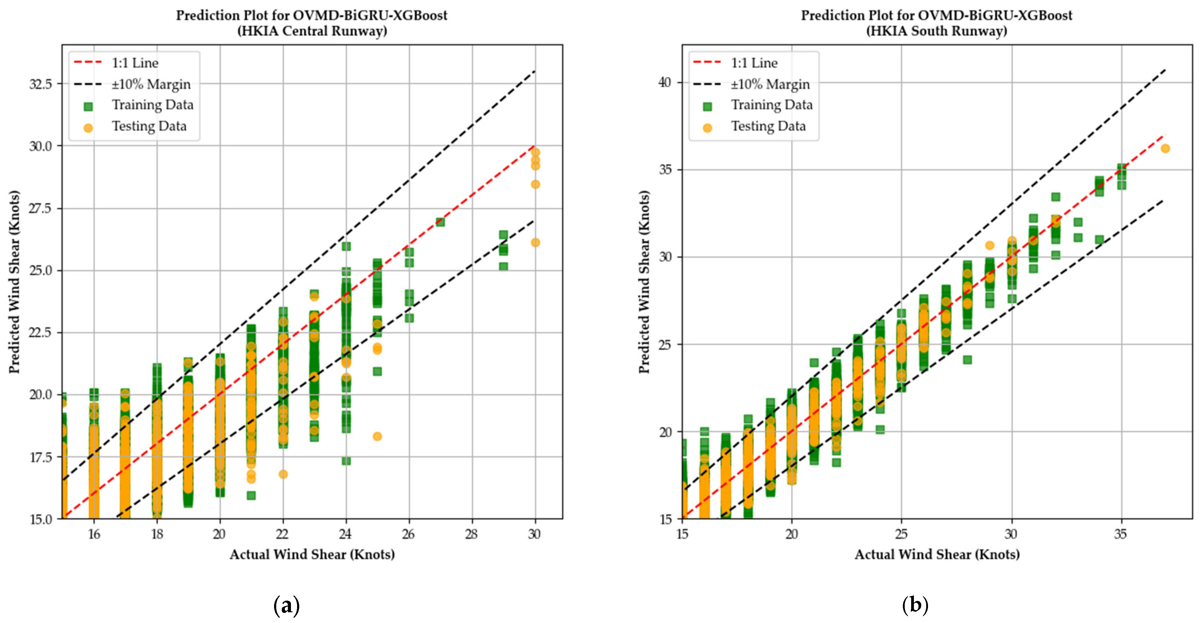
3.2. Comparison of Proposed OVMD–BiGRU–XGBoost with Other Competitive Models

Table 6. Performance comparison with different competitive deep learning models.

Model	Central Runway			South Runway
	MAE	RMSE	R2	MAE	RMSE	R2
Training data
OVMD–BIGRU–XGBoost	0.624	0.931	0.773	0.521	0.709	0.921
OVMD–GRU–XGBoost	0.705	1.042	0.712	0.593	0.821	0.884
OVMD–ResNet–XGBoost	0.794	1.201	0.648	0.681	0.933	0.836
OVMD–LSTM–XGBoost	0.682	1.015	0.719	0.571	0.789	0.895
OVMD–BiLSTM–XGBoost	0.643	0.964	0.755	0.538	0.738	0.913
Testing data
OVMD–BIGRU–XGBoost	0.624	0.931	0.729	0.521	0.709	0.926
OVMD–GRU–XGBoost	0.721	1.081	0.685	0.611	0.842	0.874
OVMD–ResNet–XGBoost	0.812	1.232	0.624	0.698	0.957	0.827
OVMD–LSTM–XGBoost	0.697	1.038	0.702	0.582	0.814	0.884
OVMD–BiLSTM–XGBoost	0.659	0.979	0.716	0.547	0.759	0.911

reports the performance of the proposed OVMD–BiGRU–XGBoost model compared with four alternative hybrid models: OVMD–GRU–XGBoost, OVMD–ResNet–XGBoost, OVMD–LSTM–XGBoost, and OVMD–BiLSTM–XGBoost. The assessment uses wind shear time series from both the central and south runways. Evaluation metrics include the MAE, RMSE, and R², with results reported for both training and testing phases. OVMD–BiGRU–XGBoost performs best across all metrics and datasets. In the central runway training data, it achieves an MAE of 0.624, RMSE of 0.931, and R² of 0.773. Its testing performance remains strong, with the same RMSE and a slightly reduced R² of 0.729. On the south runway, the model records an MAE of 0.521, RMSE of 0.709, and R² of 0.921 during training and maintains the same MAE and RMSE with an improved R² of 0.926 during testing. These results confirm its stability and ability to capture both short-term variations and broader trends.

OVMD–BiLSTM–XGBoost follows closely behind. For the central runway, it produces an MAE of 0.643, RMSE of 0.964, and R² of 0.755 in training, while in testing, it reaches an MAE of 0.659, RMSE of 0.979, and R² of 0.716. For the south runway, it records training values of MAE = 0.538, RMSE = 0.738, and R² = 0.913 and testing values of MAE = 0.547, RMSE = 0.759, and R² = 0.911. Although slightly less accurate than the proposed model, it shows a relatively close match, especially in the south runway results. OVMD–LSTM–XGBoost and OVMD–GRU–XGBoost provide moderate accuracy. On the central runway, OVMD–LSTM–XGBoost reaches an RMSE of 1.015 and R² of 0.719 in training and an RMSE of 1.038 with an R² of 0.702 in testing. OVMD–GRU–XGBoost shows slightly lower performance, with a central training RMSE of 1.042 and R² of 0.712 and testing RMSE of 1.081 with an R² of 0.685. On the south runway, OVMD–LSTM–XGBoost records RMSEs of 0.789 and 0.814 in training and testing, with R² values of 0.895 and 0.884, respectively. OVMD–GRU–XGBoost achieves higher errors in comparison, with RMSEs of 0.821 and 0.842 and R² values of 0.884 and 0.874. Among all models, OVMD–ResNet–XGBoost performs the weakest. For the central runway, its training RMSE reaches 1.201 with an R² of 0.648 and testing RMSE climbs to 1.232 with a further drop in R² to 0.624. On the south runway, training results show an RMSE of 0.933 and R² of 0.836, while testing shows an RMSE of 0.957 and R² of 0.827. These values show a limited suitability of convolution-based feature extraction for one-dimensional sequential wind shear data when compared with recurrent structures like BiGRUs and BiLSTM.

4. Conclusions and Recommendations

This study presented a hybrid modeling framework for short-term wind shear prediction at the HKIA, where complex terrain contributes to significant airflow disruptions near runways. The framework combines a signal processing approach with deep learning to improve wind shear forecasting reliability in this high wind shear risk environment. At first, the wind shear signals were decomposed using OVMD, which extracts IMFs corresponding to distinct temporal scales. Each IMF was modeled using a BiGRU to capture directional dependencies. The TPE optimization was used to tune BiGRU hyperparameters, and a residual XGBoost model refined predictions by correcting the remaining errors. The proposed hybrid OVMD–BiGRU–XGBoost model achieved strong results in testing data from both the central and south runways. For the central runway, it produced an R² of 0.729, RMSE of 0.931, and MAE of 0.624. For the south runway, R² reached 0.926, with RMSE and MAE values at 0.709 and 0.521, respectively. These results showed better predictive performance than the GRU, LSTM, BiLSTM, and ResNet-based counterparts.

Although the framework shows high accuracy, its reliance on Doppler LiDAR data may limit applicability at locations without advanced sensing infrastructure. The model was also evaluated only at the HKIA, so its behavior under different topographic and climatic conditions remains untested. Its sensitivity to rare and extreme wind shear events is another area requiring attention. Future work should examine model performance across other airports, especially those with limited meteorological data. Including variables such as vertical wind shear, temperature gradients, and pressure could provide further insight into atmospheric conditions. Additional development may focus on uncertainty estimation, probabilistic outputs, or integration into operational decision systems for aviation weather risk management.

References

1. Zhang, H.; Liu, X.; Wang, Q.; Zhang, J.; He, Z.; Zhang, X.; Li, R.; Zhang, K.; Tang, J.; Wu, S. Low-level wind shear identification along the glide path at BCIA by the pulsed coherent doppler LiDAR. Atmosphere 2020, 12, 50. [Google Scholar] [CrossRef]
2. Bretschneider, L.; Hankers, R.; Schönhals, S.; Heimann, J.-M.; Lampert, A. Wind shear of low-level jets and their influence on manned and unmanned fixed-wing aircraft during landing approach. Atmosphere 2021, 13, 35. [Google Scholar] [CrossRef]
3. International Civil Aviation Organization. Manual on Low-Level Wind Shear; International Civil Aviation Organization: Montreal, QC, Canada, 2005. [Google Scholar]
4. Federal Aviation Administration. Wind Shear; FAA-P-8740-40; Federal Aviation Administration: Washington, DC, USA, 2008. [Google Scholar]
5. Lin, C.; Zhang, K.; Chen, X.; Liang, S.; Wu, J.; Zhang, W. Overview of low-level wind shear characteristics over Chinese mainland. Atmosphere 2021, 12, 628. [Google Scholar] [CrossRef]
6. Kusuma, L.K.N.A.; Pratiwi, I.; Ismanto, H.; Fitrianto, M.A. Utilization of Doppler Weather Surveillance Radar for Wind-Shear Detection in Airport. In Proceedings of the 2022 8th International Conference on Science and Technology (ICST), Yogyakarta, Indonesia, 7–8 September 2022; pp. 1–5. [Google Scholar]
7. Ryan, M.; Saputro, A.H.; Sopaheluwakan, A. Review of low-level wind shear: Detection and prediction. AIP Conf. Proc. 2023, 2719, 020044. [Google Scholar]
8. Liu, X.; Zhang, H.; Wu, S.; Wang, Q.; He, Z.; Zhang, J.; Li, R.; Liu, S.; Zhang, X. Effects of buildings on wind shear at the airport: Field measurement by coherent Doppler lidar. J. Wind Eng. Ind. Aerodyn. 2022, 230, 105194. [Google Scholar] [CrossRef]
9. Zhang, H.; Wu, S.; Wang, Q.; Liu, B.; Yin, B.; Zhai, X. Airport low-level wind shear lidar observation at Beijing Capital International Airport. Infrared Phys. Technol. 2019, 96, 113–122. [Google Scholar] [CrossRef]
10. Gheitasi, N.; Mazlumi, F. A review on radar applications in civil aviation. In Proceedings of the 21st International Conference of Iranian Aerospace Society, Tehran, Iran, 20 February 2023; pp. 1–8. [Google Scholar]
11. MORRIS, M.T.; Brewster, K.A.; Carr, F.H. Assessing the Impact of Non-Conventional Radar and Surface Observations on High-Resolution Analyses and Forecasts of a Severe Hailstorm. Electron. J. Sev. Storms Meteorol. (EJSSM) 2021, 16, 1–39. [Google Scholar] [CrossRef]
12. Nechaj, P.; Gaál, L.; Bartok, J.; Vorobyeva, O.; Gera, M.; Kelemen, M.; Polishchuk, V. Monitoring of low-level wind shear by ground-based 3D lidar for increased flight safety, protection of human lives and health. Int. J. Environ. Res. Public Health 2019, 16, 4584. [Google Scholar] [CrossRef]
13. Mizuno, S.; Ohba, H.; Ito, K. Machine learning-based turbulence-risk prediction method for the safe operation of aircrafts. J. Big Data 2022, 9, 29. [Google Scholar] [CrossRef]
14. Khattak, A.; Chan, P.W.; Chen, F.; Peng, H. Interpretable ensemble imbalance learning strategies for the risk assessment of severe-low-level wind shear based on LiDAR and PIREPs. Risk Anal. 2024, 44, 1084–1102. [Google Scholar] [CrossRef]
15. Zhuang, Z.; Zhang, H.; Chan, P.-W.; Tai, H.; Deng, Z. A Machine Learning-Based Model for Flight Turbulence Identification Using LiDAR Data. Atmosphere 2023, 14, 797. [Google Scholar] [CrossRef]
16. Williams, J.K. Using random forests to diagnose aviation turbulence. Mach. Learn. 2014, 95, 51–70. [Google Scholar] [CrossRef] [PubMed]
17. Zhang, X.; Mahadevan, S. Ensemble machine learning models for aviation incident risk prediction. Decis. Support Syst. 2019, 116, 48–63. [Google Scholar] [CrossRef]
18. Celikmih, K.; Inan, O.; Uguz, H. Failure prediction of aircraft equipment using machine learning with a hybrid data preparation method. Sci. Program. 2020, 2020, 8616039. [Google Scholar] [CrossRef]
19. Nanduri, A.; Sherry, L. Anomaly detection in aircraft data using Recurrent Neural Networks (RNN). In Proceedings of the 2016 Integrated Communications Navigation and Surveillance (ICNS), Herndon, VA, USA, 19–21 April 2016; pp. 5C2-1–5C2-8. [Google Scholar]
20. Mamdouh, M.; Ezzat, M.; Hefny, H. Improving flight delays prediction by developing attention-based bidirectional LSTM network. Expert Syst. Appl. 2024, 238, 121747. [Google Scholar] [CrossRef]
21. Khan, W.A.; Ma, H.-L.; Chung, S.-H.; Wen, X. Hierarchical integrated machine learning model for predicting flight departure delays and duration in series. Transp. Res. Part C Emerg. Technol. 2021, 129, 103225. [Google Scholar] [CrossRef]
22. Zhu, Q.; Zhang, F.; Liu, S.; Wu, Y.; Wang, L. A hybrid VMD–BiGRU model for rubber futures time series forecasting. Appl. Soft Comput. 2019, 84, 105739. [Google Scholar] [CrossRef]
23. Khattak, A.; Chan, P.-w.; Chen, F.; Peng, H. Explainable Boosting Machine for Predicting Wind Shear-Induced Aircraft Go-around based on Pilot Reports. KSCE J. Civ. Eng. 2023, 27, 4115–4129. [Google Scholar] [CrossRef]
24. Yuen, A.; Tsui, K.; Fung, M. Hong Kong Airport’s Competitiveness as an International Hub. In Aviation Law and Policy in Asia; Brill Nijhoff: Leiden, The Netherlands, 2020; pp. 118–142. [Google Scholar]
25. Chan, P.; Hon, K. Observation and numerical simulation of terrain-induced windshear at the Hong Kong International Airport in a planetary boundary layer without temperature inversions. Adv. Meteorol. 2016, 2016, 1454513. [Google Scholar] [CrossRef]
26. Hon, K.; Chan, P. Application of LIDAR-derived eddy dissipation rate profiles in low-level wind shear and turbulence alerts at H ong K ong I nternational A irport. Meteorol. Appl. 2014, 21, 74–85. [Google Scholar] [CrossRef]
27. Chan, P. Severe wind shear at H ong K ong I nternational a irport: Climatology and case studies. Meteorol. Appl. 2017, 24, 397–403. [Google Scholar] [CrossRef]
28. Turis.io. Hong Kong Airport Departure Gate Map: Where Is My Gate? Available online: https://blog.turis.io/en/2025/01/24/hong-kong-airport-departure-gate-map-where-is-my-gate/ (accessed on 19 April 2025).
29. Lahmiri, S. A variational mode decompoisition approach for analysis and forecasting of economic and financial time series. Expert Syst. Appl. 2016, 55, 268–273. [Google Scholar] [CrossRef]
30. Chen, H.; Lu, T.; Huang, J.; He, X.; Yu, K.; Sun, X.; Ma, X.; Huang, Z. An improved VMD-LSTM model for time-varying GNSS time series prediction with temporally correlated noise. Remote Sens. 2023, 15, 3694. [Google Scholar] [CrossRef]
31. Huang, J.; Ding, W. Aircraft trajectory prediction based on bayesian optimised temporal convolutional network–bidirectional gated recurrent unit hybrid neural network. Int. J. Aerosp. Eng. 2022, 2022, 2086904. [Google Scholar] [CrossRef]
32. Zhang, J.; Jiang, Y.; Wu, S.; Li, X.; Luo, H.; Yin, S. Prediction of remaining useful life based on bidirectional gated recurrent unit with temporal self-attention mechanism. Reliab. Eng. Syst. Saf. 2022, 221, 108297. [Google Scholar] [CrossRef]
33. Chen, C.; Seo, H. Prediction of rock mass class ahead of TBM excavation face by ML and DL algorithms with Bayesian TPE optimization and SHAP feature analysis. Acta Geotech. 2023, 18, 3825–3848. [Google Scholar] [CrossRef]
34. Khattak, A.; Zhang, J.; Chan, P.-W.; Chen, F. Turbulence along the runway glide path: The invisible hazard assessment based on a wind tunnel study and interpretable TPE-optimized KTBoost approach. Atmosphere 2023, 14, 920. [Google Scholar] [CrossRef]
35. Chen, T.; Guestrin, C. Xgboost: A scalable tree boosting system. In Proceedings of the 22nd ACM Sigkdd International Conference on Knowledge Discovery and Data Mining, San Francisco, CA, USA, 13–17 August 2016; pp. 785–794. [Google Scholar]
36. Zhang, J.; Chan, P.-W.; Ng, M.K.-P. Optimal-Transport-Based Positive and Unlabeled Learning Method for Windshear Detection. Remote Sens. 2024, 16, 4423. [Google Scholar] [CrossRef]
37. Zhang, J.; Chan, P.W.; Ng, M.K. LiDAR-Based Windshear Detection via Statistical Features. Adv. Meteorol. 2022, 2022, 3039797. [Google Scholar] [CrossRef]
38. Mohanty, S.; Gupta, K.K.; Raju, K.S. Comparative study between VMD and EMD in bearing fault diagnosis. In Proceedings of the 2014 9th International Conference on Industrial and Information Systems (ICIIS), Gwalior, India, 15–17 December 2014; pp. 1–6. [Google Scholar]
39. Wang, L.; Liu, Y.; Li, T.; Xie, X.; Chang, C. Short-term PV power prediction based on optimized VMD and LSTM. IEEE Access 2020, 8, 165849–165862. [Google Scholar] [CrossRef]
40. Dinda, B. Gated recurrent neural network with TPE Bayesian optimization for enhancing stock index prediction accuracy. arXiv 2024, arXiv:2406.02604. [Google Scholar]
41. Xie, D.; Sun, H.; Qi, J. A new feature extraction method based on improved variational mode decomposition, normalized maximal information coefficient and permutation entropy for ship-radiated noise. Entropy 2020, 22, 620. [Google Scholar] [CrossRef] [PubMed]
Figure 2. Signal processing-guided deep learning framework for prediction of wind shear.
Atmosphere 16 00802 g002
Figure 3. The locations of the Doppler LiDARs at the HKIA (source: [36]).
Atmosphere 16 00802 g003
Figure 4. Radial wind velocity (knots) observed by Doppler LiDAR at HKIA using PPI mode at 3° elevation and slant ranges of 350–10,000 m (source: [37]).
Atmosphere 16 00802 g004
Figure 5. Structural overview of the BiGRU network.
Atmosphere 16 00802 g005
Figure 6. Time series of wind shear magnitudes at HKIA with data split: (a) central runway with 85% training (red), 15% testing (gray); (b) south runway with 85% training (blue), 15% testing (gray).
Atmosphere 16 00802 g006
Figure 7. Statistical characterization of wind shear magnitudes at HKIA runways: (a) histogram with KDE—central runway; (b) histogram with KDE—south runway; (c) monthly violin plots—central runway; (d) monthly violin plots—south runway; (e) hourly average—central runway; (f) hourly average—south runway; (g) yearly violin plots—central runway; (h) yearly violin plots—south runway.
Atmosphere 16 00802 g007aAtmosphere 16 00802 g007b
Figure 8. VMD-based decomposition of wind shear time series into optimal six IMFs; (a) central runway; (b) south runway.
Atmosphere 16 00802 g008
Figure 9. Actual vs. predicted IMF components using OMD–BiRGRU–XGBoost model: (a) IMF-1—central runway; (b) IMF-1—south runway; (c) IMF-2—central runway; (d) IMF-2—south runway; (e) IMF-3—central runway; (f) IMF-3—south runway; (g) IMF-4—central runway; (h) IMF-4—south runway; (i) IMF-5—central runway; (j) IMF-5—south runway; (k) IMF-6—central runway; (l) IMF-6—south runway.
Atmosphere 16 00802 g009aAtmosphere 16 00802 g009b
Figure 10. Reconstructed plot wind shear prediction performance using the OVMD–BiGRU–XGBoost model: (a) central runway; (b) south runway.
Atmosphere 16 00802 g010
Figure 11. Prediction error plots based on the OVMD–BiGRU–XGBoost model: (a) central runway; (b) south runway.
Atmosphere 16 00802 g011