
Effect of Vegetation on the Intensity of Low-Level Coastal Jets: The Case of Tenerife


Abstract
1. Introduction
1.1. Aim of the Research
1.2. General Characteristics of Low-Level Coastal Jets
1.3. Influence of Vegetation on Land Temperature
2. Materials and Methods
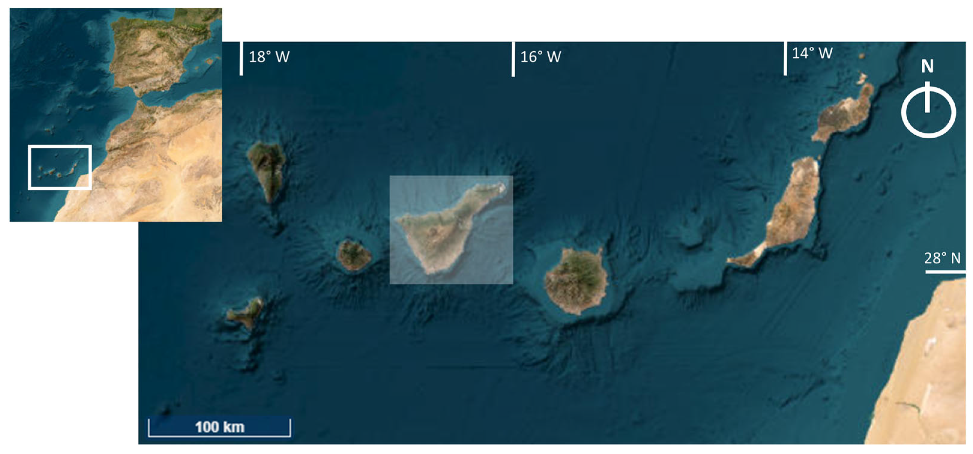
2.1. The Canary Islands, Environmental Conditions
- A wet and stable MBL as a result of upwelling;
- The presence of a persistent thermal inversion;
- An orographic barrier close to the coast, which is also subject to drastic diurnal thermal variations due to high insolation;
- Dynamic and orographic local regulators, which act on near-surface wind intensity.
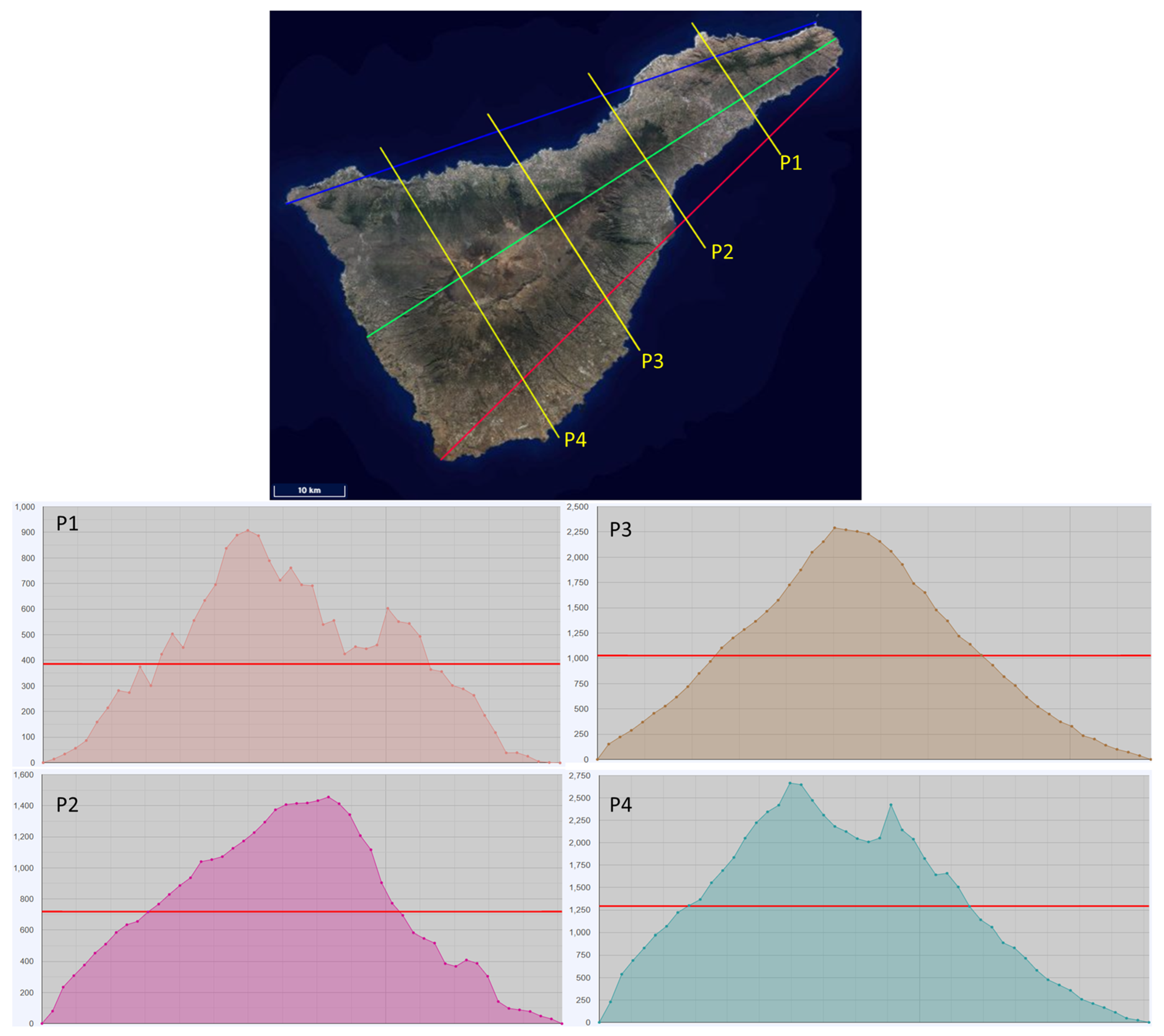
2.2. The Study Area of Tenerife
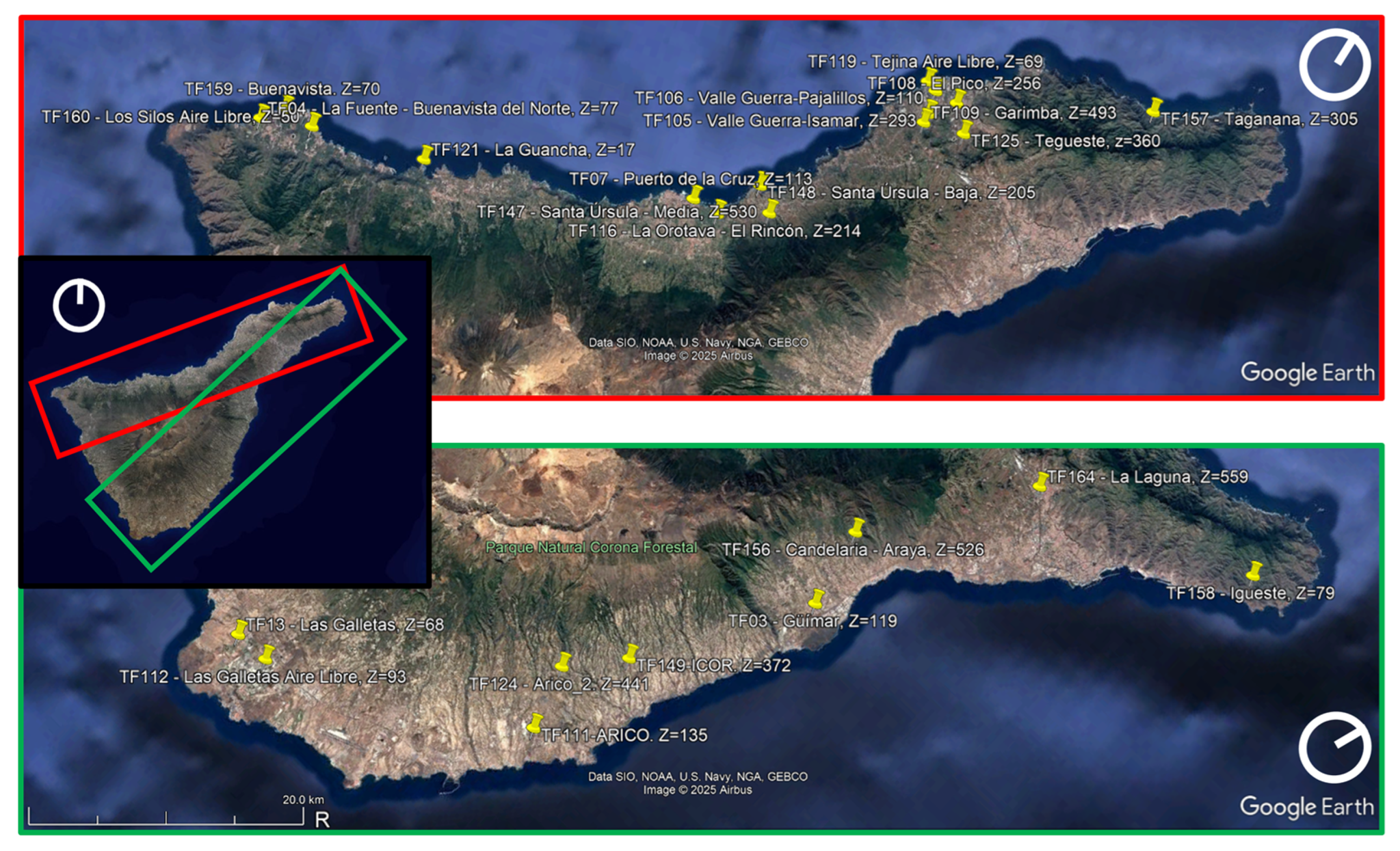
2.3. Wind Records
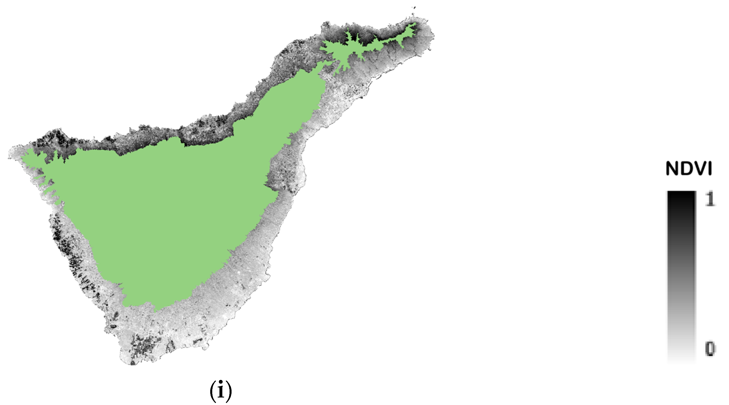
2.4. NDVI
3. Results
3.1. Wind Data
- Wads: the whole-day average speed in the period 1 June to 30 September;
- Ws9-21: the average speed in the interval between 9:00 a.m. and 9:00 p.m., when the effects of solar radiation on temperature are most apparent;
- Ws21-9: the average speed in the interval between 9:00 p.m. and 9:00 a.m., which is typically the coldest part of the day, and with a decrease in wind speed values.
3.2. NDVI Calculations
3.3. Relationship Between Wind Values and Vegetation Index
4. Discussion
- The obtained NDVI values for each facade (Table 3) align with theoretical expectations: those corresponding to the northern facade are higher. The region’s topography, characterized by rugged orography, plays a pivotal role in the retention of humid winds [35], thereby establishing the optimal conditions for substantial vegetation growth in the north [17]. Conversely, on the southeast side, where the climate is warmer and drier, the ecosystem has adapted to these conditions, resulting in significantly lower NDVI values.
- Seasonal mean wind speeds (Table 1 and Table 2) fall within expected summer ranges for this maritime climate zone, consistent with documented human adaptations to these persistent environmental conditions. A comparison of the two facades reveals notable differences, with the southeast side exhibiting significantly higher wind speeds compared to the north side.
- As illustrated in Table 4, the increase in speed during the day is more pronounced on the southernmost facade. This facade is the one with the lowest NDVI.
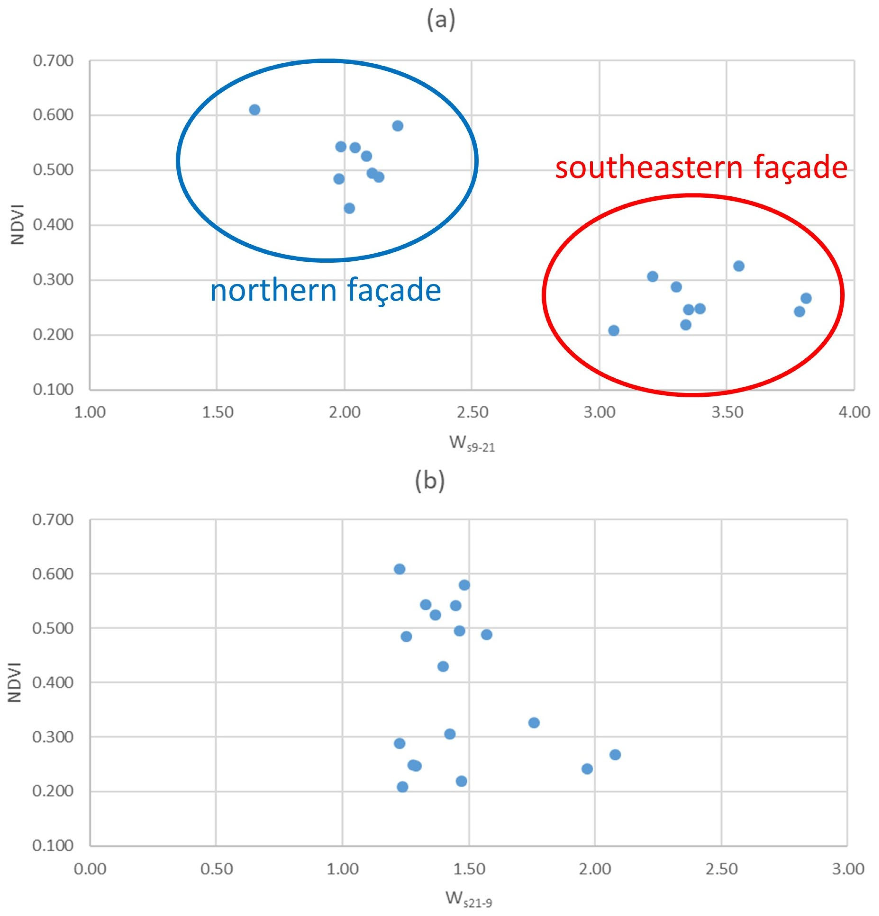
- In the graphs corresponding to Figure 5, it can be seen how during daylight hours, the pairs of wind velocity–NDVI data are grouped according to the face to which they belong. In contrast, during the night, this distinction is not clear. For all the years under study, the averages of the diurnal records on the southern facade have been clearly higher. The differences in NDVI between both areas do not affect the mean nighttime wind speed, which is similar.
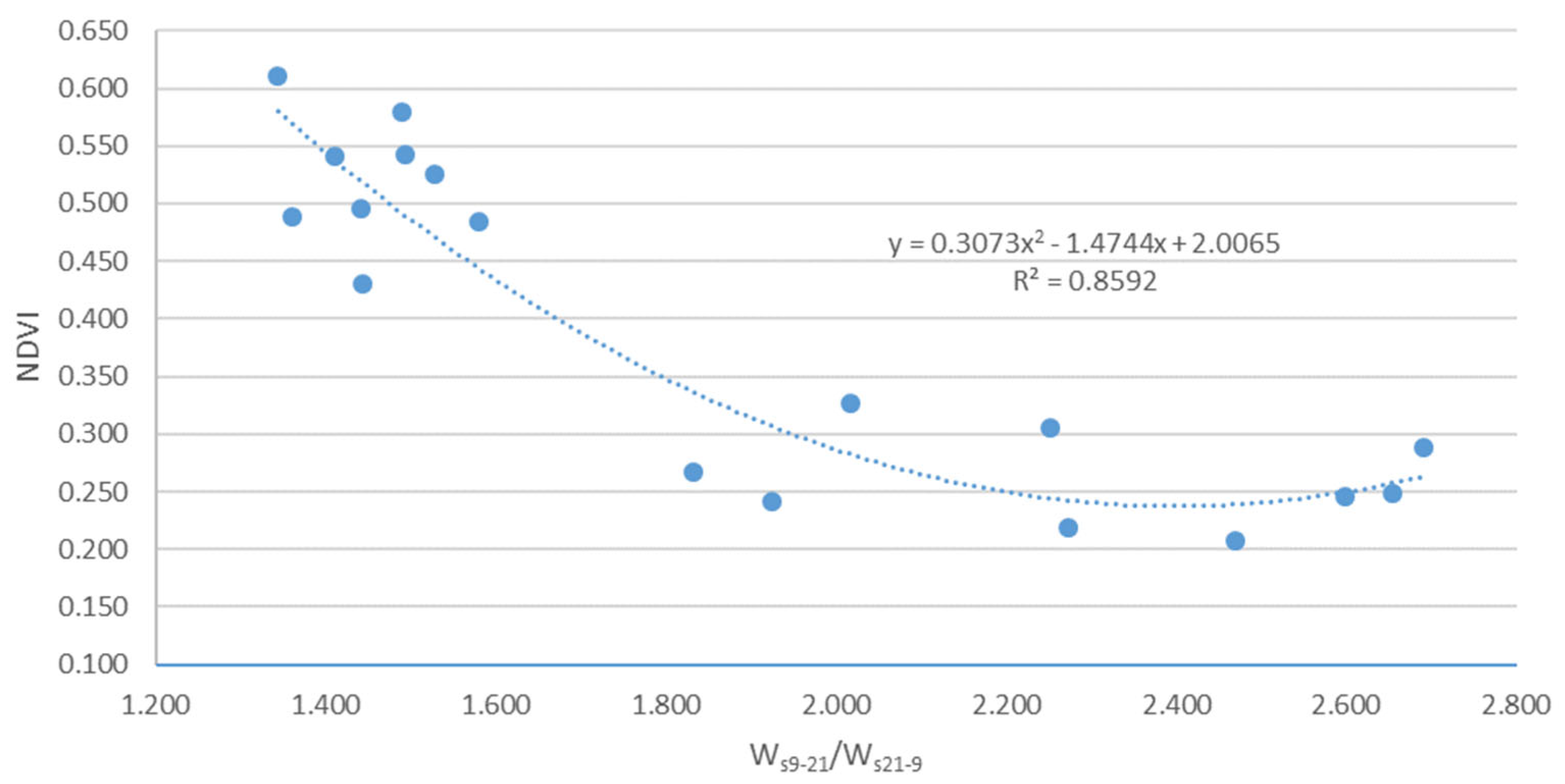
- While the years we studied are not sufficient to ensure statistical correlations of significance, Figure 6 indicates a relationship between lower NDVI values and greater increases in diurnal velocity with respect to nocturnal velocity. This will likely become more apparent as more years of study are added. This result is in agreement with the relationship between the existence of extensive vegetation cover and the difficulty of occurrence of LLCJs in the northern part of Tenerife, previously mentioned by the AEMET in the work already cited above [1].
- It should be reminded that since the records have been taken by agro-climatic stations, the situation and elevation of the anemometers with respect to the floor are not optimal for this type of study. Finally, this work has not taken into account the sea breeze circulation and the effect of its possible change of day–night breeze direction.
5. Conclusions
Author Contributions
Funding
Institutional Review Board Statement
Informed Consent Statement
Data Availability Statement
Conflicts of Interest
References
- Fernández Villares, J.; Fernández González, S. Jets Costeros En Gran Canaria y Tenerife. Caracterización y Mejora de La Predicción. Sexto Simp. Nac. Predicción Meml. Antonio Mestre 2019, 1, 223–240. [Google Scholar] [CrossRef]
- Hu, M.Q.; Mao, F.; Sun, H.; Hou, Y.Y. Study of Normalized Difference Vegetation Index Variation and Its Correlation with Climate Factors in the Three-River-Source Region. Int. J. Appl. Earth Obs. Geoinf. 2011, 13, 24–33. [Google Scholar] [CrossRef]
- Zhang, T.; Xu, X.; Jiang, H.; Qiao, S.; Guan, M.; Huang, Y.; Gong, R. Widespread Decline in Winds Promoted the Growth of Vegetation. Sci. Total Environ. 2022, 825, 153682. [Google Scholar] [CrossRef]
- Yu, M.; Wu, B.; Zeng, H.; Xing, Q.; Zhu, W. The Impacts of Vegetation and Meteorological Factors on Aerodynamic Roughness Length at Different Time Scales. Atmosphere 2018, 9, 149. [Google Scholar] [CrossRef]
- Luiz, E.W.; Fiedler, S. Global Climatology of Low-Level-Jets: Occurrence, Characteristics, and Meteorological Drivers. J. Geophys. Res. Atmos. 2024, 129, e2023JD040262. [Google Scholar] [CrossRef]
- Muñoz, R.C.; Garreaud, R.D. Dynamics of the Low-Level Jet off the West Coast of Subtropical South America. Mon. Weather Rev. 2005, 133, 3661–3677. [Google Scholar] [CrossRef]
- Lima, D.C.A.; Soares, P.M.M.; Semedo, A.; Cardoso, R.M. A Global View of Coastal Low-Level Wind Jets Using an Ensemble of Reanalyses. J. Clim. 2018, 31, 1525–1546. [Google Scholar] [CrossRef]
- Chao, S.-Y. Coastal Jets in the Lower Atmosphere. J. Phys. Oceanogr. 1985, 15, 361–371. [Google Scholar] [CrossRef]
- Winant, C.D.; Dorman, C.E.; Friehe, C.A.; Beardsley, R.C. The Marine Layer off Northern California: An Example of Supercritical Channel Flow. J. Atmos. Sci. 1988, 45, 3588–3605. [Google Scholar] [CrossRef]
- Schueler, A.; Oliveira, T.R. Influence of Vegetation on the Climate. J. Environ. Prot. 2023, 14, 725–741. [Google Scholar] [CrossRef]
- Siddiqui, A.; Maske, A.B.; Khan, A.; Kar, A.; Bhatt, M.; Bharadwaj, V.; Kant, Y.; Hamdi, R. An Urban Climate Paradox of Anthropogenic Heat Flux and Urban Cool Island in a Semi-Arid Urban Environment. Atmosphere 2025, 16, 151. [Google Scholar] [CrossRef]
- Song, Y.T.; Zhou, D.W.; Zhang, H.X.; Li, G.; Jin, Y.H.; Li, Q. Effects of Vegetation Height and Density on Soil Temperature Variations. Chinese Sci. Bull. 2013, 58, 907–912. [Google Scholar] [CrossRef]
- Troll, V.R.; Carracedo, J.C. The Canary Islands: An Introduction; Elservier: Amsterdam, The Netherlands, 2016; ISBN 9780128096635. [Google Scholar] [CrossRef]
- Negredo, A.M.; van Hunen, J.; Rodríguez-González, J.; Fullea, J. On the Origin of the Canary Islands: Insights from Mantle Convection Modelling. Earth Planet. Sci. Lett. 2022, 584, 117506. [Google Scholar] [CrossRef]
- Bechtel, B. The Climate of the Canary Islands by Annual Cycle Parameters. In Proceedings of the International Archives of the Photogrammetry, Remote Sensing and Spatial Information Sciences—ISPRS Archives, Prague, Czech Republic, 12–19 July 2016; Volume 41, pp. 243–250. [Google Scholar]
- Cuevas-Agulló, E.; Barriopedro, D.; García, R.D.; Alonso-Pérez, S.; González-Alemán, J.J.; Werner, E.; Suárez, D.; Bustos, J.J.; García-Castrillo, G.; García, O.; et al. Sharp Increase in Saharan Dust Intrusions over the Western Euro-Mediterranean in February–March 2020–2022 and Associated Atmospheric Circulation. Atmos. Chem. Phys. 2024, 24, 4083–4104. [Google Scholar] [CrossRef]
- Del Arco Aguilar, M.J.; Rodríguez Delgado, O. Vegetation of the Canary Islands; Springer International Publishing: Cham, Switzerland, 2018; ISBN 9783319772547. [Google Scholar]
- Marcello, J.; Eugenio, F.; Medina, A. Analysis of Regional Vegetation Changes with Medium and High Resolution Imagery. Remote Sens. Agric. Ecosyst. Hydrol. XIV 2012, 8531, 85311R. [Google Scholar] [CrossRef]
- Puig-Samper, M.Á.; Rebok, S. Sentir y Medir: Alexander von Humboldt En España; Doce Calles SL: Aranjuez, Madrid, 2007; ISBN 9788497440653. [Google Scholar]
- von Humboldt, A.; Bonpland, A. Atlas Geographique et Physique Du Nouveau Continent; F. Schoell: Paris, France, 1814. [Google Scholar]
- Fernandez-Palacios, J.M.; Arévalo, J.R.; Delgado, J.D.; Otto, R. Canarias. Ecología, Medio Ambiente y Desarrollo; Centro de la Cultura Popular Canaria: La Laguna, Islas Canarias, España, 2004; ISBN 84-7926-454-3. [Google Scholar]
- Bramwell, D. Flora de Las Islas Canarias; Editorial Rueda: Madrid, España, 1997; ISBN 8472071022. [Google Scholar]
- Gobierno de Canarias Red Canaria de Espacios Naturales Protegidos. Available online: https://www3.gobiernodecanarias.org/medusa/ (accessed on 3 March 2025).
- Gobierno de Canarias Superficie Cultivada Según Grupos de Productos Agrícolas y Sistemas de Cultivo. Municipios e Islas de Canarias. Desde 2007. Available online: https://www3.gobiernodecanarias.org/istac/statistical-visualizer/ (accessed on 3 March 2025).
- Gómez, J.M.N.; Lousada, S.; Velarde, J.G.; Castanho, R.A.; Loures, L. Land-Use Changes in the Canary Archipelago Using the CORINE Data: A Retrospective Analysis. Land 2020, 9, 232. [Google Scholar] [CrossRef]
- European Commission Factsheet on 2014-2022 Rural Development Programme for the Canary Islands. 2024. Available online: https://agriculture.ec.europa.eu/system/files/2022-08/rdp-factsheet-spain-canarias_en.pdf (accessed on 4 March 2025).
- Megías, E.; García-Román, M. Influence of Trade Winds on the Detection of Trans-Hemispheric Swells near the Canary Islands. Atmosphere 2022, 13, 505. [Google Scholar] [CrossRef]
- Ministerio de Agricultura, P. y A.G. de E. Sistema de Información Agroclimática Del Regadío. Available online: https://www.mapa.gob.es/es/desarrollo-rural/temas/gestion-sostenible-regadios/sistema-informacion-agroclimatica-regadio/presentacion.aspx (accessed on 13 April 2025).
- Gilabert, M.; González-Piqueras, J.; García-Haro, J. Acerca de Los Índices de Vegetación. Rev. Teledetección 1997, 8, 1–10. [Google Scholar]
- Muñoz, P. Apuntes de Teledetección: Índices de Vegetación; Centro de Información de Recursos Naturales: Santiago de Chile, Chile, 2013. [Google Scholar]
- Vladimir, J.; Zurita, S. Relación Entre El Índice de Vegetación NDVI, Temperatura Superficial y Radiación Solar En Áreas Urbanas de La Parroquia Calderón, Quito, Ecuador, Analizada En Base de Teledetección Relationship between NDVI Vegetation Index, Surface Temperature and S. Latam Rev. Latinoam. De Cienc. Soc. Y Humanidades 2025, 6, 43. [Google Scholar]
- Devendran, A.A.; Banon, F. Spatio-Temporal Land Cover Analysis and the Impact of Land Cover Variability Indices on Land Surface Temperature in Greater Accra, Ghana Using Multi-Temporal Landsat Data. J. Geogr. Inf. Syst. 2022, 14, 240–258. [Google Scholar] [CrossRef]
- Fabeku, B.B.; Balogun, I.A.; Adegboyega, S.A.-A.; Faleyimu, O.I. Spatio-Temporal Variability in Land Surface Temperature and Its Relationship with Vegetation Types over Ibadan, South-Western Nigeria. Atmos. Clim. Sci. 2018, 08, 318–336. [Google Scholar] [CrossRef]
- Pérez, B.; Serna, A.; Delgado, J.; Caballero, M.; Villa, G. El Programa Copernicus Para La Monitorización Del Territorio y Los Objetivos Del Desarrollo Sostenible; Centro Nacional de Información Geográfica: Madrid, España, 2022. [Google Scholar]
- García-Alvarado, J.J.; Bello-Rodríguez, V.; González-Mancebo, J.M.; Del Arco, M.J. Updating Knowledge of Vegetation Belts on a Complex Oceanic Island after 20 Years under the Effect of Climate Change. Biodivers. Conserv. 2024, 33, 2441–2463. [Google Scholar] [CrossRef]


| Year | Wads | Ws9-21 | Ws21-9 |
|---|---|---|---|
| 2016 | 1.52 | 1.65 | 1.23 |
| 2017 | 1.73 | 1.98 | 1.25 |
| 2018 | 1.82 | 2.09 | 1.37 |
| 2019 | 1.92 | 2.21 | 1.48 |
| 2020 | 1.92 | 2.14 | 1.57 |
| 2021 | 1.83 | 2.02 | 1.40 |
| 2022 | 1.83 | 2.04 | 1.45 |
| 2023 | 1.78 | 1.99 | 1.33 |
| 2024 | 1.90 | 2.11 | 1.46 |
| Average speed | 1.81 | 2.02 | 1.39 |
| Year | Wads | Ws9-21 | Ws21-9 |
|---|---|---|---|
| 2016 | 2.52 | 3.21 | 1.43 |
| 2017 | 2.64 | 3.34 | 1.47 |
| 2018 | 2.56 | 3.35 | 1.29 |
| 2019 | 2.51 | 3.30 | 1.23 |
| 2020 | 2.34 | 3.06 | 1.24 |
| 2021 | 3.09 | 3.79 | 1.97 |
| 2022 | 3.14 | 3.81 | 2.08 |
| 2023 | 2.86 | 3.55 | 1.76 |
| 2024 | 2.62 | 3.40 | 1.28 |
| Average speed | 2.70 | 3.42 | 1.53 |
| Year * | Face | Mean | Deviation | Max. | Min. ** |
|---|---|---|---|---|---|
| 2016 | North | 0.610 | 0.221 | 0.940 | 0.000 |
| Southeast | 0.306 | 0.185 | 0.939 | 0.000 | |
| 2017 | North | 0.484 | 0.204 | 0.940 | 0.000 |
| Southeast | 0.219 | 0.155 | 0.939 | 0.000 | |
| 2018 | North | 0.525 | 0.232 | 0.940 | 0.000 |
| Southeast | 0.246 | 0.174 | 0.939 | 0.000 | |
| 2019 | North | 0.580 | 0.224 | 0.940 | 0.000 |
| Southeast | 0.288 | 0.176 | 0.939 | 0.000 | |
| 2020 | North | 0.488 | 0.206 | 0.940 | 0.000 |
| Southeast | 0.208 | 0.157 | 0.939 | 0.000 | |
| 2021 | North | 0.430 | 0.248 | 0.940 | 0.000 |
| Southeast | 0.242 | 0.170 | 0.939 | 0.000 | |
| 2022 | North | 0.541 | 0.221 | 0.940 | 0.000 |
| Southeast | 0.267 | 0.181 | 0.939 | 0.000 | |
| 2023 | North | 0.543 | 0.206 | 0.940 | 0.000 |
| Southeast | 0.326 | 0.017 | 0.939 | 0.000 | |
| 2024 | North | 0.495 | 0.209 | 0.940 | 0.000 |
| Southeast | 0.248 | 0.160 | 0.939 | 0.000 |
| Year | NDVI | Ws9-21 | Ws21-9 | Ws9-21/ Ws21-9 |
|---|---|---|---|---|
| Northern facade: | ||||
| 2016 | 0.610 | 1.65 | 1.23 | 1.343 |
| 2017 | 0.484 | 1.98 | 1.25 | 1.579 |
| 2018 | 0.525 | 2.09 | 1.37 | 1.528 |
| 2019 | 0.580 | 2.21 | 1.48 | 1.491 |
| 2020 | 0.488 | 2.14 | 1.57 | 1.360 |
| 2021 | 0.430 | 2.02 | 1.40 | 1.443 |
| 2022 | 0.541 | 2.04 | 1.45 | 1.410 |
| 2023 | 0.543 | 1.99 | 1.33 | 1.493 |
| 2024 | 0.495 | 2.11 | 1.46 | 1.441 |
| Southwestern facade: | ||||
| 2016 | 0.306 | 3.21 | 1.43 | 2.251 |
| 2017 | 0.219 | 3.34 | 1.47 | 2.274 |
| 2018 | 0.246 | 3.35 | 1.29 | 2.599 |
| 2019 | 0.288 | 3.30 | 1.23 | 2.690 |
| 2020 | 0.208 | 3.06 | 1.24 | 2.469 |
| 2021 | 0.242 | 3.79 | 1.97 | 1.924 |
| 2022 | 0.267 | 3.81 | 2.08 | 1.832 |
| 2023 | 0.326 | 3.55 | 1.76 | 2.016 |
| 2024 | 0.248 | 3.40 | 1.28 | 2.655 |
Disclaimer/Publisher’s Note: The statements, opinions and data contained in all publications are solely those of the individual author(s) and contributor(s) and not of MDPI and/or the editor(s). MDPI and/or the editor(s) disclaim responsibility for any injury to people or property resulting from any ideas, methods, instructions or products referred to in the content. |
© 2025 by the authors. Licensee MDPI, Basel, Switzerland. This article is an open access article distributed under the terms and conditions of the Creative Commons Attribution (CC BY) license (https://creativecommons.org/licenses/by/4.0/).
Share and Cite
Megías, E.; García-Román, M. Effect of Vegetation on the Intensity of Low-Level Coastal Jets: The Case of Tenerife. Atmosphere 2025, 16, 801. https://doi.org/10.3390/atmos16070801
Megías E, García-Román M. Effect of Vegetation on the Intensity of Low-Level Coastal Jets: The Case of Tenerife. Atmosphere. 2025; 16(7):801. https://doi.org/10.3390/atmos16070801
Chicago/Turabian StyleMegías, Emilio, and Manuel García-Román. 2025. "Effect of Vegetation on the Intensity of Low-Level Coastal Jets: The Case of Tenerife" Atmosphere 16, no. 7: 801. https://doi.org/10.3390/atmos16070801
APA StyleMegías, E., & García-Román, M. (2025). Effect of Vegetation on the Intensity of Low-Level Coastal Jets: The Case of Tenerife. Atmosphere, 16(7), 801. https://doi.org/10.3390/atmos16070801