Large Eddy Simulation of the Diurnal Cycle of Shallow Convection in the Central Amazon

Abstract

Climate models often face challenges in accurately simulating the daily precipitation cycle over tropical land areas, particularly in the Amazon. One contributing factor may be the incomplete representation of the diurnal evolution of shallow cumulus (ShCu) clouds. This study aimed to enhance the understanding of the diurnal cycles of ShCu clouds—from formation to maturation and dissipation—over the Central Amazon (CAMZ). Using observational data from the Green Ocean Amazon 2014 (GoAmazon) campaign and large eddy simulation (LES) modeling, we analyzed the diurnal cycles of six selected pure ShCu cases and their composite behavior. Our results revealed a well-defined cycle, with cloud formation occurring between 10 and 11 local time (LT), maturity from 13 to 15 LT, and dissipation by 17–18 LT. The vertical extent of the liquid water mixing ratio and the intensity of the updraft mass flux were closely associated with increases in turbulent kinetic energy (TKE), enhanced buoyancy flux within the cloud layer, and reduced large-scale subsidence. We further analyzed the diurnal cycles of the convective available potential energy (CAPE), the convective inhibition (CIN), the Bowen ratio (BR), and the vertically integrated TKE in the mixed layer (ITKE-ML), exploring their relationships with the cloud base mass flux (Mb) and cloud depth across the six ShCu cases. ITKE-ML and Mb exhibited similar diurnal trends, peaking at approximately 14–15 LT. However, no consistent relationships were found between CAPE (or BR) and Mb. Similarly, comparisons of the cloud depth with CAPE, BR, ITKE-ML, CIN, and Mb revealed no clear relationships. Smaller ShCu clouds were sometimes linked to higher CAPE and lower CIN. It is important to emphasize that these findings are preliminary and based on a limited sample of ShCu cases. Further research involving an expanded dataset and more detailed analyses of the TKE budget and synoptic conditions is necessary. Such efforts would yield a more comprehensive understanding of the factors influencing ShCu clouds’ vertical development.

1. Introduction

The Amazon rainforest, the world’s largest tropical forest, experiences diverse atmospheric conditions that produce various convective cloud types, including shallow cumulus (ShCu), congestus, and deep convective clouds. ShCu clouds were identified as the most prevalent clouds during the GoAmazon 2014/15 campaign [1]. These clouds play a crucial role in the vertical transport of heat, moisture, and momentum from the lower atmosphere to the mid-troposphere. Additionally, they precondition the atmosphere, creating favorable conditions for the transition from shallow to deep convection. This transition significantly impacts the timing and intensity of the diurnal cycle of precipitation (DCP). However, the current climate models face challenges in accurately simulating the DCP over land, especially in the Amazon. Previous studies suggest that the inaccuracies over land may partly stem from the inadequate representation of shallow cumulus and congestus clouds and the pivotal role of cold pools in facilitating the transition from shallow to deep convection in atmospheric models [2,3,4,5,6,7,8,9].

Numerous observational field campaigns across various regions have significantly advanced our understanding of shallow clouds. Notable campaigns over the Atlantic Ocean include the Atlantic Tradewind Experiment (ATEX [10]), the Barbados Oceanographic Meteorological Experiment (BOMEX [11]), Rain in Shallow Cumulus over the Ocean (RICO [12]), and more recently, the EURE4CA campaign, which explores cloud–circulation coupling in the climate system [13]. Over land, essential observations have been provided by the ARM-SGP observatory [14], the Routine AAF CLOWD Optical Radiative Observations (RACORO [15]), and the GoAmazon experiment in Central Brazil [16]. These initiatives have significantly advanced our understanding of the primary characteristics of ShCu clouds and have improved the development of ShCu parameterizations [17,18,19,20,21,22,23,24].

Previous studies in the Central Amazon (e.g., [1,24,25]) and Southwestern Amazon (e.g., [26,27,28,29]) underscore the need to better understand the physical processes that drive the formation of ShCu clouds and their transition to deep convection. Tang et al. [30] leveraged data from the GoAmazon campaign, applying a constrained variational objective analysis approach to create initial conditions and large-scale forcings suitable for cloud resolving models (CRM) and large eddy simulations (LES). In addition, Tang et al. [24] utilized these large-scale forcings to examine the diurnal cycle of precipitation over the Amazon using 11 single-column models (SCMs). They identified a common issue among the models: the premature onset of afternoon precipitation, attributed to difficulties in accurately capturing the transition from shallow to deep convection.

Tian et al. [25] examined the interplay of surface fluxes, atmospheric humidity, wind shear, and entrainment in influencing the transition from shallow to deep convection during the GoAmazon 2014/5 field campaign in the Amazon. For ShCu convection, their results showed that ShCu days exhibit higher sensible heat fluxes, promoting boundary layer growth, entraining drier free-tropospheric air, and higher cloud bases compared to deep convection days. Additionally, precipitating ShCu clouds were more frequently observed on days associated with deep convection. Building on the role of surface fluxes, Grabowski [31] investigated the influence of surface forcing, particularly the partitioning of surface heat fluxes into sensible and latent components, represented by the Bowen ratio, in the Southern Amazon. The study demonstrated that the Bowen ratio critically affects the surface buoyancy flux, the evolution of the daytime convective boundary layer, and the transition from shallow to deep convection over land. These findings underscore the importance of surface heat flux partitioning in shaping cloud formation and convective processes. Despite these insights, to our knowledge, no LES simulations have yet been conducted to examine the development of non-precipitation pure shallow cumulus (as defined in Section 2) in the Central Amazon.

Understanding the development of ShCu clouds, especially over the Amazon, and accurately incorporating these processes into parameterizations is vital in addressing the shortcomings in simulating the DCP in climate models. Although our primary motivation is to study ShCu clouds and DCP over land, this study focuses on improving our understanding of the diurnal cycle of ShCu in the Central Amazon, utilizing an LES model alongside observational data from the GoAmazon campaign. LES models have become a powerful tool for planetary boundary layer and ShCu research, providing detailed insights that are often missing from observational studies. Additionally, they have played a key role in the development of various ShCu parameterizations (e.g., [19,32,33,34,35,36,37,38]).

This paper is organized as follows. Section 2 describes the model, dataset, and methodology. Section 3, Section 3.2, and Section 3.4 discuss the results from the LES simulations. Finally, in Section 4, conclusions are given.

2. Model Description, Data, and Design of Numerical Experiments

2.1. Model Description

The model used for the LES simulations is the System for Atmospheric Modeling (SAM v.6.10.6, [39]). SAM is a non-hydrostatic model that solves the 3D anelastic momentum, continuity, and tracer conservation equations. We use the bulk microphysics single moment [39], the subgrid-scale turbulence first-order closure [40], and the radiation package based on the radiation scheme from the National Center for Atmospheric Research Community Atmosphere Model version 3 [41]. The lateral boundary conditions in both horizontal directions are periodic, and the upper boundary is a rigid lid. Following the BOMEX shallow convection cases used in the LES inter-comparison study [32], random perturbations with amplitudes of 0.1 K for the temperature and 0.025 g kg⁻¹ for the specific humidity are added to the lowest model levels.

The simulations are conducted on a numerical domain of 1200 × 1200 × 150 grid points, with uniform grid spacing of ${\Delta }_x={\Delta }_y=100$ m in the horizontal direction and ${\Delta }_z=50$ m in the vertical direction, using a time step of ${\Delta }_t=1$ s. To ensure robustness, sensitivity tests are performed with various horizontal grid resolutions of 50, 100, 150, and 200 m. These tests indicate that the variations in grid resolution do not significantly affect the results, demonstrating the model’s stability across different resolutions. Based on these findings, and in alignment with previous studies focused on the Amazon region [27,29], we select a grid resolution of 100 m for our simulations. This resolution and physical configuration strike a balance between computational efficiency and the accuracy needed to represent the physical processes of pure warm non-precipitating ShCu convection. Future work aims to incorporate double-moment microphysics schemes, which provide prognoses for hydrometeors’ number concentration and mass. These advanced schemes are expected to enhance the accuracy of cloud property representations, including droplet size distributions and aerosol–cloud interactions. Such improvements may significantly influence shallow clouds’ lifetimes and their interactions with the broader atmospheric environment.

The simulation domain approximates the pentagonal area of the Intensive Observation Periods (IOPs) (see Figure 1, for which large-scale forcings were developed by Tang et al. [30], as detailed in Section 2.2. The simulations begin at sunrise, around 06 local time (LT, UTC-4), as in the approach used in previous LES and SCM studies over ARM-SGP by Brown et al. [33] and Guichard et al. [2]. This start time is approximately three to four hours before the onset of daytime shallow cloud formation, allowing the model to capture the early morning boundary layer evolution and the subsequent development of shallow cumulus clouds.

2.2. Large-Scale Forcing Data

Large-scale forcing (horizontal moisture and temperature advection tendencies and horizontal and vertical wind components), initial conditions (temperature and water vapor), and surface flux datasets developed by Tang et al. [30] for the two GoAmazon IOPs are used. These values are similar to those used by Song and Zhang [37] and Tang et al. [24]. These datasets represent a spatial average over the octagonal area shown in Figure 1 (hereafter referred to as Central Amazon—CAMZ) centered at Manaus Ponta Pelada Airport (3.15° S and 59.99° W). The prescribed large-scale forcing profiles and the prescribed latent and sensible heat flux data are available every three hours; the model interpolates to each time step during 14 h (6–20 LT) of the complete-time simulation.

2.3. Methodology Used to Search ShCu Cases

This section presents the process carried out to identify the days with pure ShCu, referred to here as ShCu cases, during the wet season (from 15 February to 26 March 2014) and dry season (September and October 2014) of the GoAmazon IOPs (80 days). A ShCu case is defined as a day with shallow convective clouds within 8 to 18 h LT, representing the ShCu population in the CAMZ. No other convective clouds (congestus or deep) should be found within this period. However, ShCu could coexist with clouds at the middle and high levels, such as altostratus, altocumulus, or cirrus clouds. The steps to select ShCu cases are explained below.

First, as an initial estimate, the cloud masking dataset from the ARM site (Figure 1) was used to identify days with ShCu cases over the ARM site. Cloud masking and the derivation of products were performed using the 95 GHz W-band ARM cloud radar (WACR) multi-sensor and preprocessing using remote sensing cloud methodologies [1]. According to the height of the cloud boundaries and the cloud thickness, these data classify clouds into seven categories: shallow, congestus, deep convection, altocumulus, altostratus, cirrostratus/anvil, and cirrus. This dataset identified 12 days of pure ShCu (12 ShCu cases) over the ARM site in both IOPs. Figure 1a illustrates one of the selected ShCu cases, with shallow cumulus clouds (red color), overlying altostratus (cyan blue), and without congestus or deep convective clouds during its development from 9 to 15 LT on 10 March 2014 in IOP1.

Second, we assume that the 12 ShCu cases selected over the ARM site or T3 are representative of the CAMZ’s shallow cloud properties based on previous studies by Giangrande et al. [1]. They compared ShCu between T3 ground-based and satellite observations, and their results suggest that the ShCu observed over the ARM site represent the larger-domain cloud properties within a few hundred kilometers. Nevertheless, congestus or deep convective clouds outside the ARM site for these 12 ShCu cases cannot be ruled out. One of the principal characteristics of shallow cumulus is low rain or no rain; therefore, to reduce these uncertainties, hourly precipitation data in CAMZ are used, as shown in Figure 1b,c, for the wet and dry seasons, respectively, during the IOPs [30]. Although the ShCu maximum rainfall intensity remains uncertain [42,43,44], we used a maximum rainfall threshold of 0.4 mmh⁻¹ (identified by the red line in Figure 1b,c) as a constraint to exclude days with possible congestus or deep convective clouds in the CAMZ. This threshold of 0.4 mmh⁻¹ is based roughly on Arulraj and Barros [43] [Figure 1b]. They revealed a wide range of ShCu rain rates at the ARM TMP, whereas the rain rate was generally less than 0.5 mmh⁻¹. From both constraints, the cloud masking and rain rate, 9 days with pure ShCu were selected.

2.4. LES Simulations to Choose ShCu Cases

We assume that these 9 days with ShCu at the ARM site represent shallow cumulus in the CAMZ domain. However, this selection does not exclude the possibility that one or more of these selected days also includes other convective clouds, such as congentus or deep convection, in a broader ARM site region extending into the CAMZ. For instance, Collow and Miller [45] showed that the nearby rivers (Amazon and Rio Negro) contributed to spatial variability in the regional radiation budgets around the ARM site. The abundant moisture transport by breezes can be favorable for the local ShCu development around the ARM site. Therefore, some of the 9 ShCu selected might be local clouds. Similarly, the rain threshold, about 0.4 mmh⁻¹, does not guarantee the existence of isolated congestus or deep convection within the CAMZ domain.

One way to reduce these uncertainties is by determining the maximum cloud top height (h_top) and cloud fraction (CF) through LES simulations for the nine selected days. These constraints are as follows: 1.5 km < h_top < 4 km and 3% < CF < 25% at 13–14 LT. With these restrictions, finally, six active ShCu cases representative of the Central Amazon were selected (Mar10, Sep3, Sep11, Oct1, Oct5, and Oct8). Figure 2 shows various diurnal cloud characteristics. The initial formation of ShCu clouds occurred between 9 and 10 LT on some days (Mar10, Oct5, and Oct8) and between 11 and 12 LT on others (Sep3, Sep11, and Oct1).

Additionally, another LES simulation was carried out using the composite data for the six cases. This composite shallow cumulus is referred to in this paper as composite ShCu. The initial conditions, large-scale forcing, and surface fluxes for the composite ShCu dataset were created by averaging the datasets from the six cases. Figure 3 depicts the initial conditions in terms of the potential temperature and specific humidity (a), large-scale forcing wind (b), vertical velocity component (c), horizontal and vertical advection of potential temperature (d), and specific humidity (e) for this composite ShCu. The initial conditions and forcings for the six selected cases (figure not shown) are overall akin to those in Figure 3.

The vertical profiles of the potential temperature and specific humidity at the initial conditions for the selected and composite ShCu cases (Figure 3a) do not show the typical inversion layer at the cloud top (around 2–3 km). Previous studies of shallow cumulus overland areas [33,37] suggest that the absence of inversion would produce computational noise at high levels (e.g., 5–7 km) because of the presence of the mid-level clouds. Initially, we introduced an inversion layer in our setup by modifying the potential temperature gradient for the Amazon ShCu case, creating an inversion above 4 km. However, comparisons between simulations with and without adjustments to the initial temperature profiles revealed a minimal impact on the results. Consequently, we excluded this artificial inversion in the final simulations. The initial conditions and large-scale forcing for the composite ShCa are available through the links in the Data Availability Statement.

Comparing our results with and without changes in the temperature profiles does not substantially modify our results. Figure 4 presents the daily cycle of the surface sensible heat flux (a), the surface latent heat flux (b), and the ratio of surface sensible to surface latent heat fluxes (Bowen ratio) (c) (the ratio of sensible heat flux to latent heat flux) for the six ShCu cases and the composite ShCu case.

3. Results of Large Eddy Simulations

3.1. Cloud Fraction, Liquid Water, and Updraft Mass Flux Vertical Profiles

Since continental ShCu clouds are inherently transient, this section details their development from initiation to dissipation, encompassing the stages of initiation, maturation, and dilution. The evolution of ShCu onset, growth, and dissipation is analyzed using the cloud fraction (CF) and liquid water content (LW) for the composite case. As shown in Figure 5, the initiation stage occurs around 10–11 LT, when ShCu clouds first appear. Peak values of approximately 9% define the maturation stage for CF and 0.02 g kg⁻¹ for LW, reaching around 13–15 LT. The dissipation stage follows, with the clouds fading before sunset, around 17–18 LT. Figure 5a shows a gradual increase in the cloud base height, rising from about 0.5 km during initiation to approximately 1.0 km at maturation. In contrast, the cloud top heights exhibit more rapid growth, increasing from about 1.0 km at 9–11 LT to roughly 3.0 km at 13–15 LT.

Figure 6, Figure 7 and Figure 8 present the diurnal variation in the CF, LW cloud fraction, and updraft mass flux (uMF) vertical profiles, respectively, with different lines and colors representing several hours for the six ShCu cases (a–f) and the composite ShCu case (g). The cloud fraction profiles (Figure 6) capture the diversity in the ShCu cloud sizes, providing insights into the range of cloud structures observed. The results indicate that ShCu formation begins earlier, around 9–10 LT, in certain cases (e.g., Oct5 and Oct8), whereas the composite case (Figure 6g) shows fully developed clouds by 10–11 LT, which is consistent with Figure 5a. The CF (Figure 6), LW (Figure 7), and uMF (Figure 8) reach their peak values above the cloud base between 13 and 15 LT, followed by a decline approaching sunset at around 17 LT, which is also consistent with the trends observed in Figure 5a. The increase in CF and LW during the dissipation phase, particularly at approximately 4 km in the Mar10 case (Figure 6a and Figure 7a), likely reflects the presence of altostratus clouds (as indicated by Figure 2a). In contrast, the persistently high CF and LW values during the dissipation phase in the Oct1 case may have resulted from delayed ShCu onset (11–12 LT) and a later maturation phase (14–15 LT) than in other cases.

The vertical profiles of uMF and CF share a similar structure throughout the ShCu life cycle, with higher values near the cloud base and lower values near the cloud top. Their intensities decrease gradually with the height, starting from a peak just above the cloud base and reaching nearly zero at the cloud top at different times during the evolution of the ShCu clouds. A notable exception occurs in the Oct5 case from 13 to 15 LT, where these variables show an increase around the mid-cloud level, which is attributed to the maximum LW values at this altitude (Figure 8e), resulting in a slightly altered profile compared with those of the other cases.

The close relationship between the CF and uMF in the SAM arises from how the uMF is defined as a function of the cloud fraction (${\sigma }_u$), the cloud vertical velocity component ($w_u$), and the air density ($\rho$), following the formulation of Arakawa and Schubert [46]: $uMF=\rho {\sigma }_u{w}_u$. In our experiments, the $w_u$ vertical profile (figure not shown) remains nearly constant with the height. Given that the air density does not vary significantly within the cloud layer, this relationship explains why the vertical profiles of CF and uMF exhibit similar shapes. This behavior is consistent with findings from recent observational studies, including those from ARM campaigns [47,48,49], Darwin, Australia [50], studies over tropical oceans [51], the NARVAL2 campaign [52], and global analyses using satellite and ground-based data [53]. These observations support the applicability of the Arakawa and Schubert [46] formulation in the SAM.

3.2. Buoyancy Flux (B), Subcloud Mixed Layer (ML), and Entrainment (E) and Detrainment (D) Rates

Figure 9a–g show the daily variation in the buoyancy flux (B) profiles. $B=g/{\theta }_0\overline{w^{\prime }{\theta }_v^{\prime }}$, where g is gravity, w is the vertical velocity component, ${\theta }_v$ is the virtual potential temperature, and ${\theta }_0$ represents the reference-state potential temperature. The over-bar denotes space and temporal averaging, and the prime symbol indicates fluctuations from the mean. Figure 10 shows a schematic view of the ShCu based on the CF (Figure 6g) and buoyancy flux profiles (Figure 9g) for the composite case. Figure 9a,b illustrate the CF and B at different local times—for instance, at 13 LT (red color line) and 15 LT (orange color line). The cloud layer, uMF, subcloud mixed layer (ML), cloud base height (h_base), cloud top height (h_top), lifting condensation level (LCL), and the level of free convection (LFC) are defined for 15 LT.

The ML is the subcloud layer between the top surface layer and approximate ShCu cloud base level. The minimum buoyancy flux level identifies the ML_top level [33,54]. For example, in Figure 10b, the minimum B level at 13 LT is around 0.9 km. It is the ML_top level. Although there is a thin transition layer between the ML_top level and cloud base level (LCL), the ML_top and cloud base levels are considered at the same level. For instance, comparing B (Figure 9b) and CF (Figure 9a) at 15 LT, we can see that the cloud base and minimum value of B are approximately at the same level. Some thermals reach their minimum negative buoyancy (ML_top level), and some of them can ascend above the LFC (B > 0), forming the active ShCu. The cloud top is defined at the neutral buoyancy level, at height of approximately 3 km height.

Figure 9, aided by Figure 10b, illustrates the diurnal cycle of the buoyancy flux in the mixed layer and the cloud layer. In Figure 9, the positive vertical turbulent buoyancy flux in the ML decreases linearly with the height until it reaches the neutral buoyancy level, where the flux crosses zero (B = 0). This reduction in buoyancy flux is driven by surface heating, which serves as the primary driver of convective turbulence in the subcloud layer. Additionally, Figure 9 shows that B reaches its peak value in the subcloud layer near the surface across all ShCu cases during the cloud maturation stage, around 13–15 LT. Following this peak, B decreases sharply, reaching its minimum during dissipation at 17–18 LT. Conversely, within the cloud layer, B increases with the height in the lower part, peaking at around 13–15 LT due to latent heat release from condensation processes (reflected in the increasing LW in Figure 7). Beyond this point, B gradually decreases with the height due to entrainment, until it reaches the neutral buoyancy level near the cloud top.

Now, we briefly analyze the entrainment and detrainment processes that regulate the exchange of air masses between clouds and their surrounding environment. Figure 11a,b illustrate the diurnal variation in the bulk plume fractional entrainment ($ϵ$) and detrainment ($\delta$) rates, respectively, for the composite case. These rates are calculated using the formulas $ϵ$ = E/uMF and $\delta$ = D/uMF, where E and D represent the entrainment and detrainment rates (kgm⁻³s⁻¹), respectively. The values of E and D are estimated following the methodologies described in [19,55,56] and [57] (Equations (11) and (12) in [57] ). Figure 11a illustrates the fractional entrainment rates during different stages of cloud evolution. During the initiation stage, the entrainment rate peaks near the cloud base. In the maturity stage, it remains high near the cloud base (approximately 2 km⁻¹) and decreases with the height. However, the rate increases near the cloud top during the dissipation stage. On average (black line), the fractional entrainment rate closely resembles the profile observed during the maturity stage and aligns with results from the BOMEX stationary case [19]. Figure 11b shows that the fractional detrainment rates are generally greater than the fractional entrainment rates, consistent with other LES studies, such as those for the BOMEX [19] and SGP ARM [58] cases. Overall, fractional detrainment increases with the height after maturity, reaching maximum values of approximately 4 km⁻¹.

The parameterization of the entrainment rates in ShCu convection, particularly within mass flux schemes, remains a critical yet challenging problem. Despite significant advances in kilometer-scale numerical modeling, shallow convection parameterization remains indispensable because these processes occur at sub-grid scales that models cannot explicitly resolve. Various factors influence entrainment, including the cloud depth, subcloud thermodynamics, and environmental humidity. Lu et al. [59] provided valuable insights into entrainment rate parameterizations for ShCu, emphasizing the importance of integrating observational data with large eddy simulation results to improve the accuracy. Their study highlighted the variability in the entrainment rates and stressed the need for refined approaches. Innovative schemes, such as those incorporating buoyancy sorting [60], have shown considerable potential in improving entrainment rate parameterizations. Additionally, machine learning techniques have emerged as a promising approach, offering the capability to dynamically predict the entrainment rates based on varying environmental conditions [61]. In future work, we will evaluate various entrainment rate parameterizations for ShCu over the Central Amazon, benchmarking them against the LES results, in alignment with the approach proposed by Lu et al. [59].

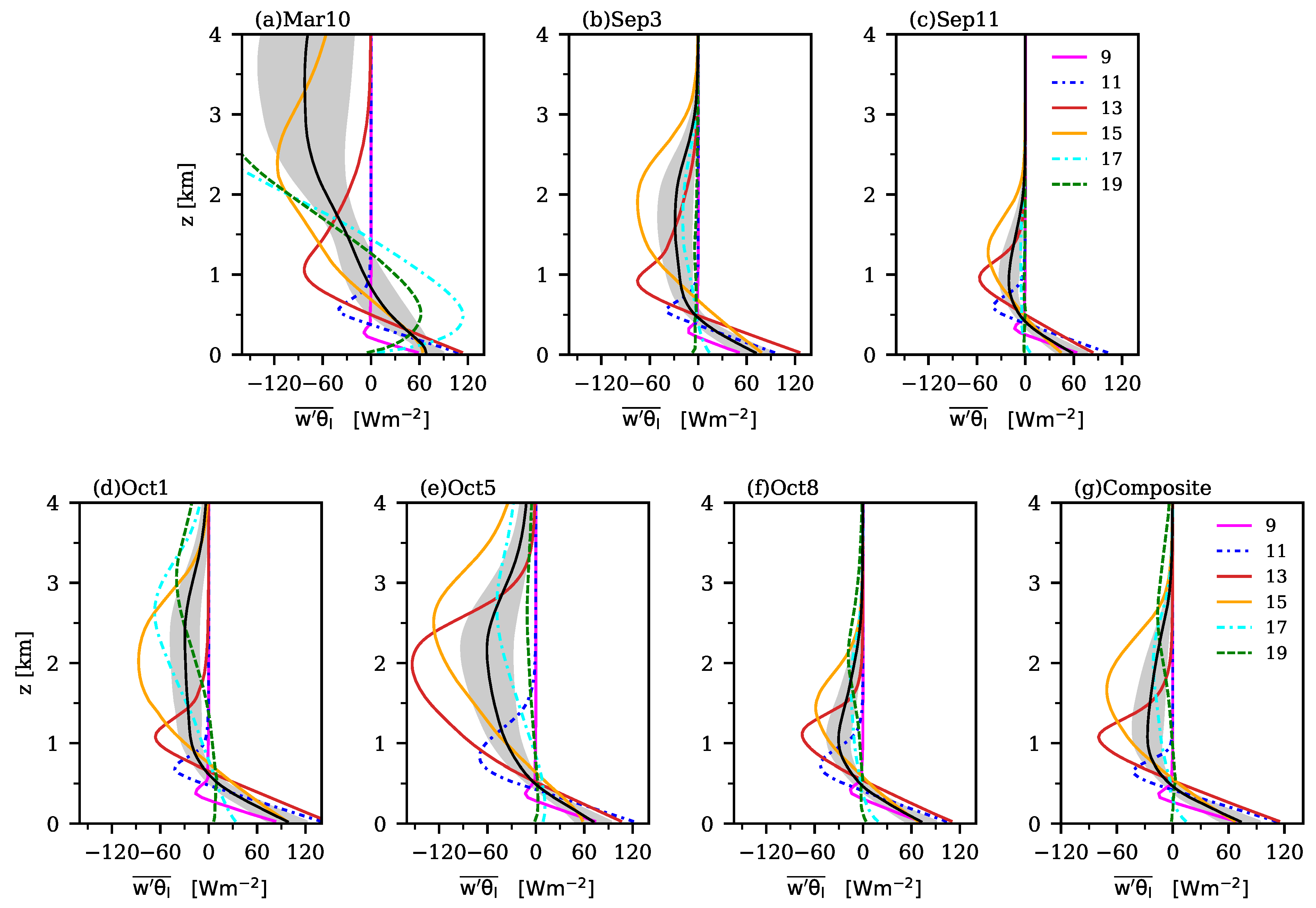
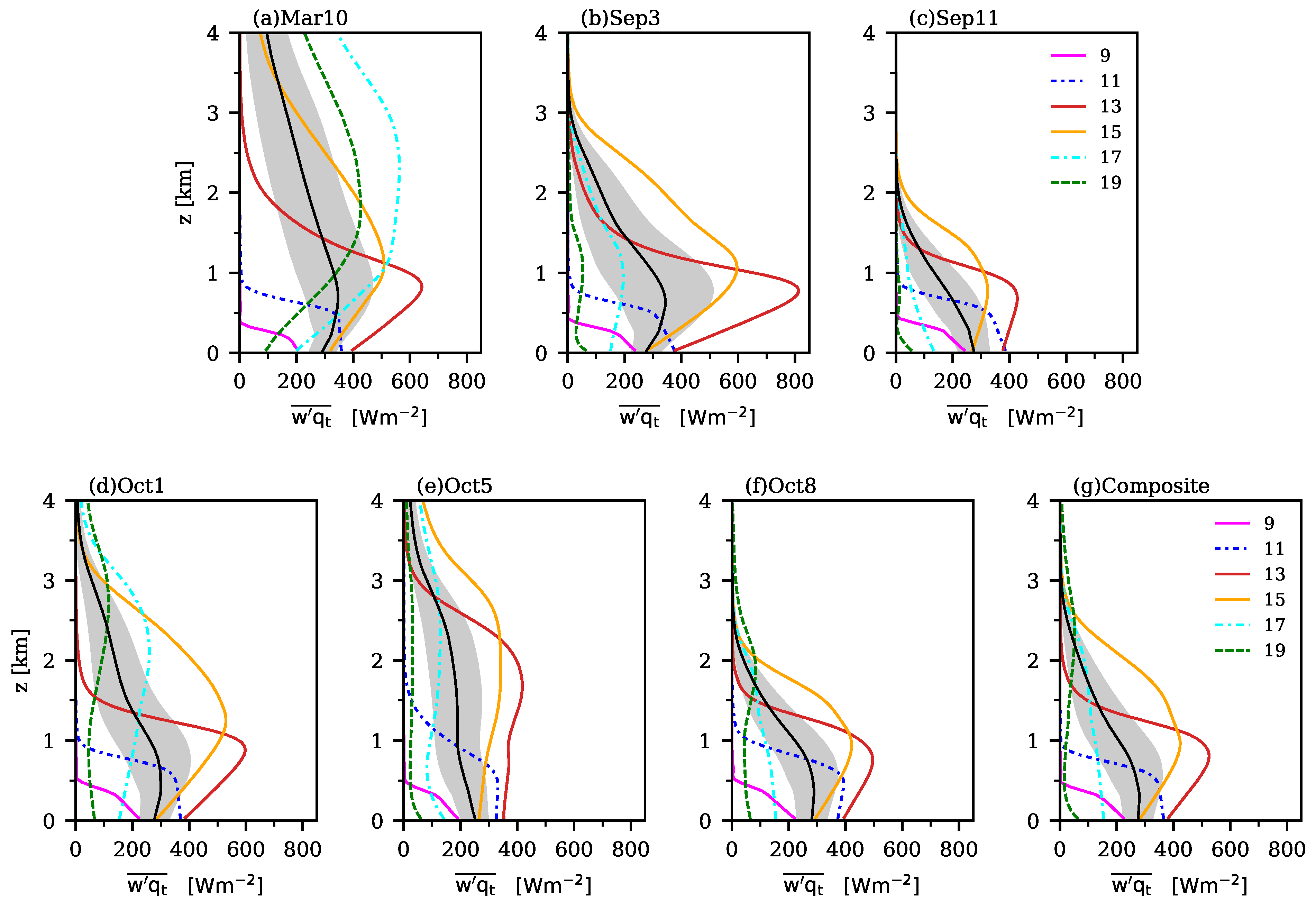
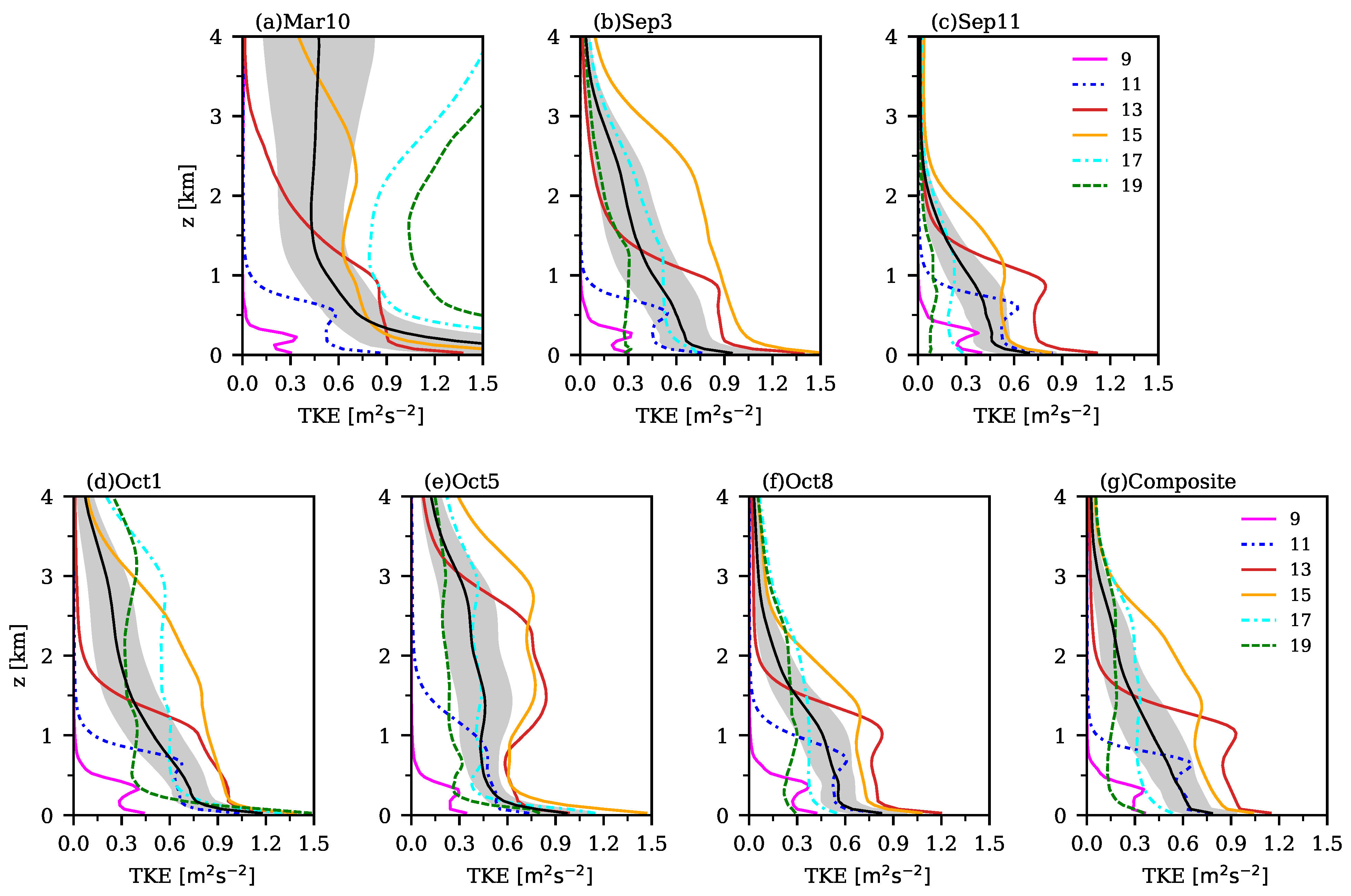
3.3. Vertical Heat and Moisture Fluxes and TKE Profiles

Figure 12 and Figure 13 show the vertical profiles of the conservative variables, liquid water potential (${\theta }_l$) flux ($\overline{w^{\prime }{\theta }_l^{\prime }}$), and total water ($q_t$) flux ($\overline{w^{\prime }{q}_t^{\prime }}$), respectively. Here, ${\theta }_l\approx \theta -\theta L/\left(C_{p}T\right)q_l$ (as defined by Betts [17]), where L is the latent heat of the vaporization of water, $q_t=q_l+q_v$, $q_t$ is the liquid water specific humidity, and $q_v$ is the water vapor specific humidity. Figure 12 shows that the positive heat fluxes near the surface decrease linearly with the height until they reach their minimum values at the maximum LW level (Figure 7). For instance, in the case of Oct5 (Figure 12b), the minimum value of heat flux and the maximum value of LW (Figure 7b) at 13–15 LT (red and orange lines) are at the same level, at about 2.0–2.5 km. Since the $\overline{w^{\prime }{\theta }_l^{\prime }}$ depends on $\overline{w^{\prime }{\theta }^{\prime }}$ and $\overline{w^{\prime }{q}_l^{\prime }}$ ($\overline{w^{\prime }{\theta }_l^{\prime }}=\overline{w^{\prime }{\theta }^{\prime }}-\overline{w^{\prime }{q}_l^{\prime }}$), the minimum heat flux is related to the maximum evaporation in the cloud layer.

The vertical moisture transport (Figure 13) from the ML into the cloud layers can be divided into two steps. One is that $\overline{w^{\prime }{q}_t^{\prime }}$ increases with the height in the ML at a linear rate, until approximately the ML_top level and cloud base level, where most of the moisture coming from the subcloud layer via the ML updraft plumes is deposited. For example, at 13 LT (red line), the maximum moisture fluxes are near the cloud base at around 0.75 km (compared with the minimum B values in Figure 9), except in the case of Oct 1, where the maximum values are at about 1.0 km. In the second step, the cloud updraft plumes take away moisture from the cloud base to the high cloud layer levels, where the $\overline{w^{\prime }{q}_t^{\prime }}$ decreases with the height at a linear rate until reaching its minimum value at the cloud top.

Figure 14a–f, along with Figure 14g (composite case), depict strong subsidence throughout the initiation to maturation stages. This subsidence is particularly intense in the Sep11 and Oct8 ShCu cases, which likely contributes to their limited vertical extents. In contrast, reduced subsidence during the morning is observed in the Mar10, Oct5, and Oct1 ShCu cases, which is consistent with their greater vertical development (see CF, LW, and uMF in Figure 6, Figure 7 and Figure 8). These results suggest that strong subsidence creates unfavorable conditions for the deepening of ShCu clouds.

The diurnal variations in the turbulent kinetic energy (TKE) vertical profiles are shown in Figure 15. TKE can be used as an indicator of the turbulence intensity; in addition, its budget considers the momentum, heat, and moisture fluxes from the surface to the cloud layer, through the ML. Among the different terms that contribute to the budget of TKE, the buoyancy flux term ($\overline{w^{\prime }{\theta }_v^{\prime }}$) is one of the driving forces for turbulence in the ML and cloud layer [21,62,63]. Following [64], this term can be written as a function of the fluxes of the liquid water potential temperature $\overline{w^{\prime }{\theta }_l^{\prime }}$ and the total water ($\overline{w^{\prime }{q}_t^{\prime }}$), as $\overline{w^{\prime }{q}_t^{\prime }}=\alpha \overline{w^{\prime }{\theta }_l^{\prime }}+\beta \overline{\theta }\overline{w^{\prime }{q}_t^{\prime }}$, where $\overline{\theta }$ represents the resolved potential temperature, and $\alpha$ and $\beta$ are coefficients that are dependent on whether the atmosphere is saturated (cloudy) or unsaturated (clear sky) (details in [64], Appendix A).

Figure 15 shows the diurnal variations in the turbulent intensity during the ShCu cloud life cycle. The TKE increases (decreases) in the ML as the buoyancy flux increases (decreases) (Figure 9) from 11 LT to 13–15 LT (from 15 to 18 LT). The maximum TKE values near the cloud base level (except for the Oct5 case) decrease almost linearly with the height until their minimum values at the cloud top, similar to the uMF (Figure 8). Since the buoyancy flux ($\overline{w^{\prime }{\theta }_v^{\prime }}$) depends mainly on the moisture fluxes ($\overline{w^{\prime }{q}_t^{\prime }}$), and since the buoyancy flux is the most important producer of turbulence within ShCu clouds, the TKE and moisture flux also have similar variation with the height above the mixed-layer top during the ShCu life cycle.

The dynamics of ShCu primarily involve the interplay between the subcloud and cloud layers. The growth of the ML top height can be analyzed through the surface buoyancy flux (Bs, Figure 9), which can be approximated as a function of the surface sensible heat flux (SHF, Figure 4) and surface latent heat flux (LHF, Figure 4b). The relationship between the Bs and surface fluxes can be approximate as $Bs\approx g/\left(C_p{\rho }_s{\theta }_0\right)(SHF+0.07SLF)$, where g is gravity, $C_p$ is the specific heat at a constant pressure, and ${\theta }_0$ and ${\rho }_s$ are the potential temperature and air density references, respectively. The diurnal cycle of the vertical profiles of the potential temperature and specific humidity (figures not shown) for all cases indicates a well-mixed subcloud layer from cloud formation at about 11 LT to dissipation at around 17–18 LT, as reflected by the near-constant vertical profiles of the potential temperature and specific humidity in the ML. The daytime ML and cloud base heights increase until 13–15 LT as the ML temperature rises and moisture decreases. Both heights peak when Bs, SHF, and LHF reach their maximum values (compare Figure 5 and Figure 9g), consistent with the findings of Tian et al. [24] and Grabowski [31]. Notably, significant ML heating, drying, and the maximum Bs (Figure 9b) are observed in the Sep 3 case, while the Oct5 case exhibits less variation (Figure 9e). Interestingly, this is opposite to the observed cloud depth, suggesting that higher SHF or LHF values and higher cloud base heights do not necessarily guarantee greater vertical cloud development.

3.4. TKE, CAPE, and CIN

Considering our LES simulation results, we explore the relationship among the vertically integrated TKE in the ML (ITKE-ML), convective available potential energy (CAPE), and convective inhibition (CIN). Figure 16a–d display the daily variation in ITKE-ML, the maximum uMF (which represents approximately the cloud base mass flux, Mb), CAPE, and CIN. Figure 16a shows that, overall, ITKE-ML quickly increased from 9–10 LT until it reached its maximum value at around 14–16 LT, which is quite similar to Mb (Figure 16b) (except for the Oct5 case). Recent observational studies by Zheng and Rosenfeld [65] and Zheng et al. [66] also support that Mb can be based on subcloud layer turbulence.

Conversely, CAPE (Figure 16c) does not align with the evolution of Mb. It increases at around 12 LT, 2–3 hours before Mb reaches its peak. Furthermore, CAPE increases during the ShCu dissipation stage (except for the Sep3 case), which is much different from the Mb evolution. These results concerning CAPE for ShCu are consistent with recent studies by Raymond and Fuchs-Stone [67] and Becket et al. [68]. Similarly, the daily variation in BR (Figure 4c) for all ShCu cases and the composite ShCu showed that BR did not change during the ShCu evolution (9–18 LT). The only case in which BR and CAPE follow Mb’s evolution is the case of Sep3. Other studies suggest that Mb is controlled by the ratio of CIN and TKE in the subcloud boundary layer (e.g., [69]), and this concept has been applied in some shallow cumulus parameterizations (e.g., [60,70,71]). The evolution of the potential energy barrier, represented by CIN, is shown in Figure 16c, which illustrates a rapid decrease in CIN until it reaches its minimum between 10:00 and 13:00 LT, in contrast to the integrated TKE values. We expected higher CIN values for smaller ShCu cases (Sep11 and Oct8) and lower values for larger ShCu cases (e.g., Oct5, and Oct1); however, this figure does not show the expected relationship. As such, we cannot confirm whether this relationship holds for the smaller cases, and further study using additional cases is required. We recognize that a limitation of this study is the small number of shallow convective cases, particularly during the wet season, which includes only one case. This limitation hinders comparisons between the dry and wet seasons. For instance, Figure 2a shows medium-level clouds that differ from those observed during the dry season. However, this single wet-season case cannot be considered representative. A larger dataset is required to achieve more robust results on the differences between the dry and wet seasons. In future work, we plan to analyze an expanded dataset of ShCu cases, incorporating more wet-season cases and a wider variety of ShCu with differing cloud depths.

4. Conclusions

Climate models often struggle to simulate the diurnal cycle of precipitation accurately over tropical land, particularly in regions such as the Amazon. Previous studies suggest that this challenge is partly due to the inadequate representation of the diurnal evolution of shallow cumulus (ShCu) clouds. This study aimed to enhance the understanding of the diurnal progression of these clouds—from formation to maturation and dissipation—over the Central Amazon (CAMZ). To achieve this goal, we utilized observational data from the Green Ocean Amazon 2014 (GoAmazon) campaign and a large eddy simulation (LES) model. We selected six ShCu cases with varying vertical extents and created a composite ShCu case by averaging the initial conditions, large-scale forcing, and surface processes from these cases. The main findings are as follows.

(1)

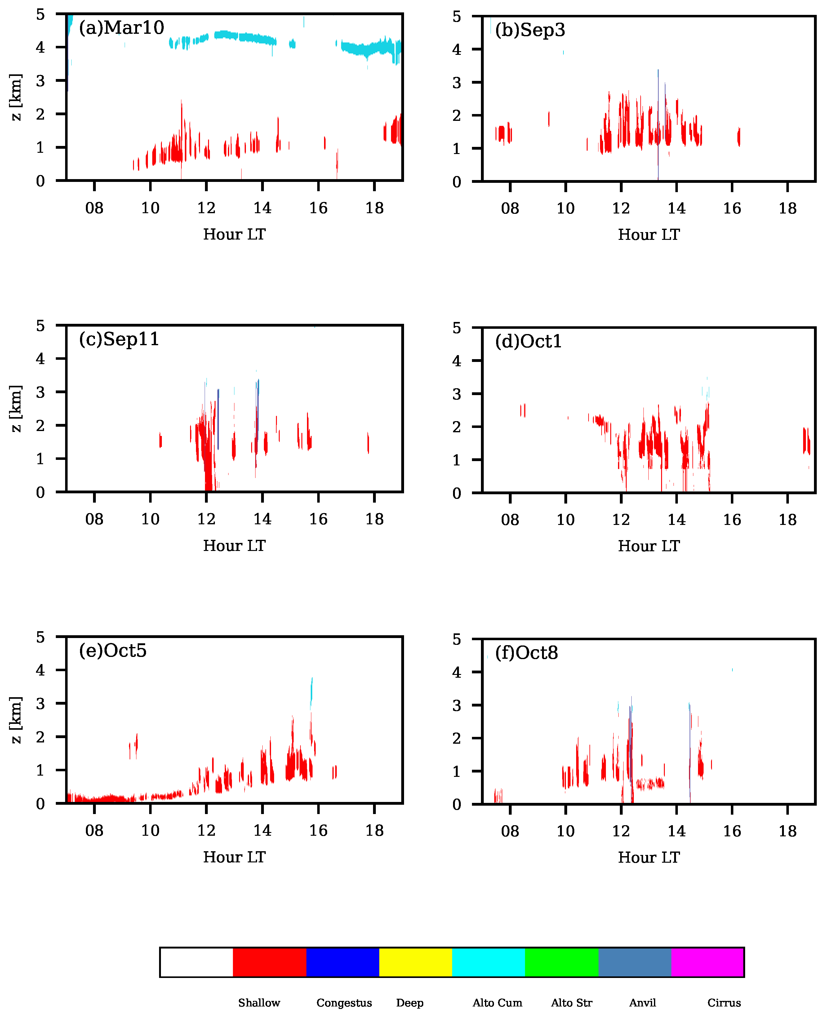
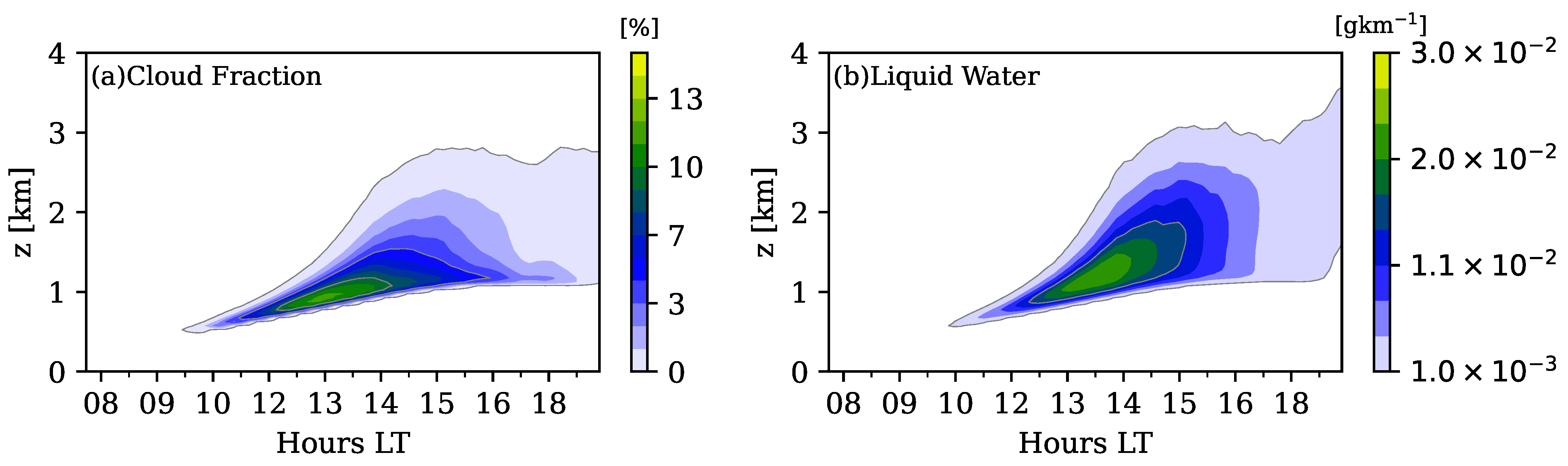
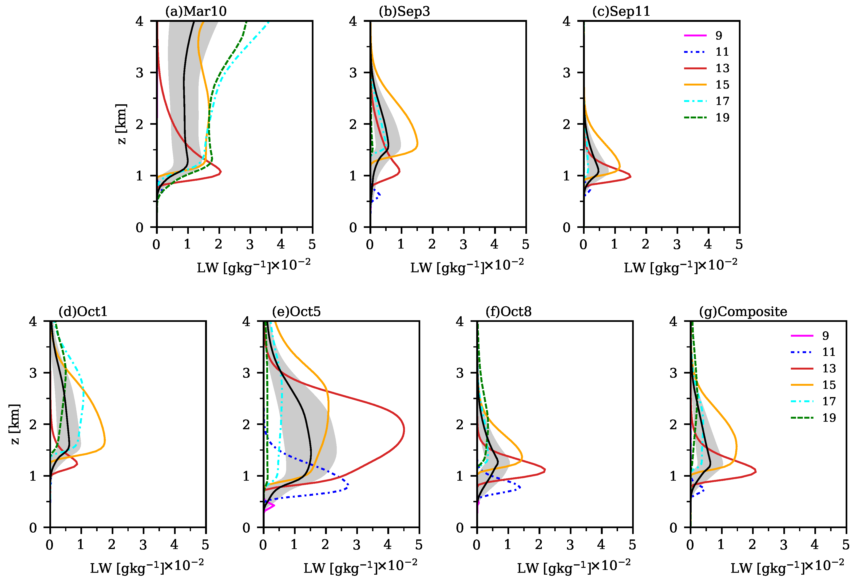
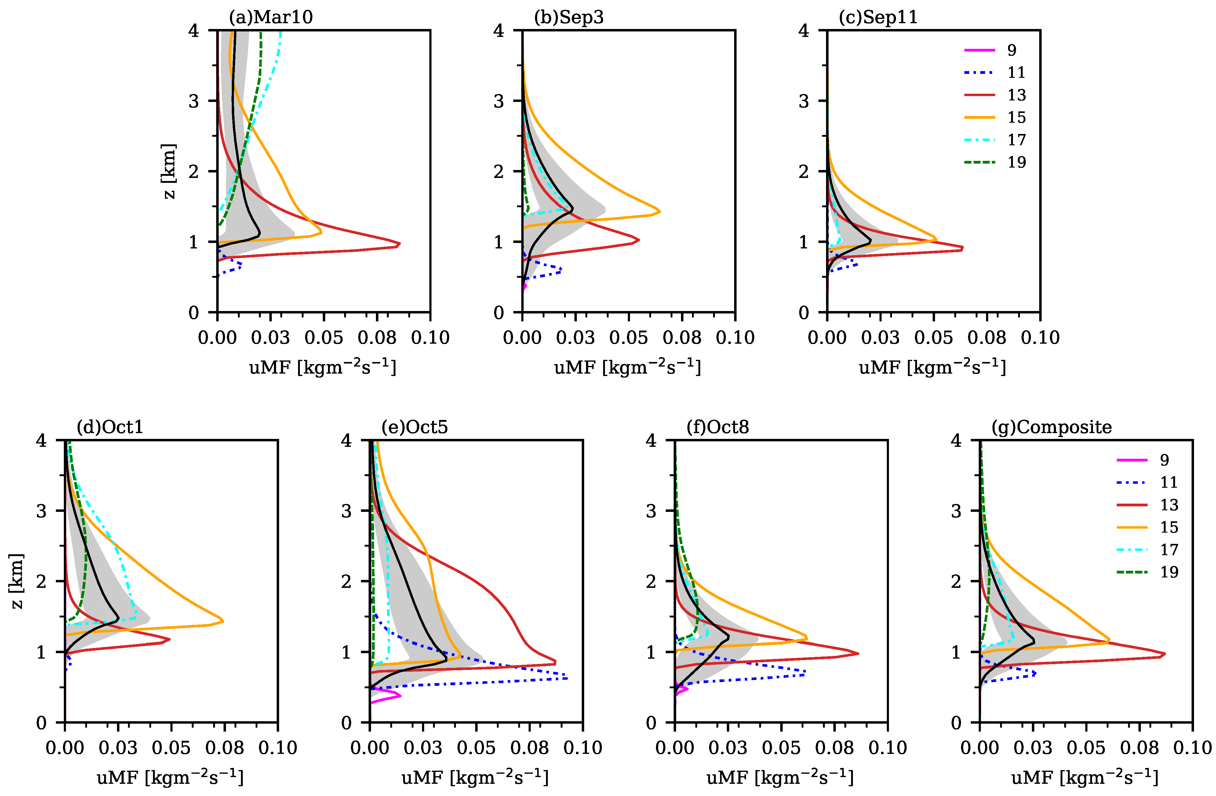
Diurnal cycle of ShCu clouds: The diurnal evolution of ShCu clouds follows a consistent pattern, initiating at approximately 10–11 LT, reaching maturity between 13 and 15 LT, and dissipating by 17–18 LT. Our results suggest that the vertical extent and intensity of the updraft mass flux and liquid water mixing ratio—as well as the deepening of the ShCu cloud layer—are closely associated with the enhanced buoyancy flux within the cloud layer and reduced large-scale subsidence.

(2)

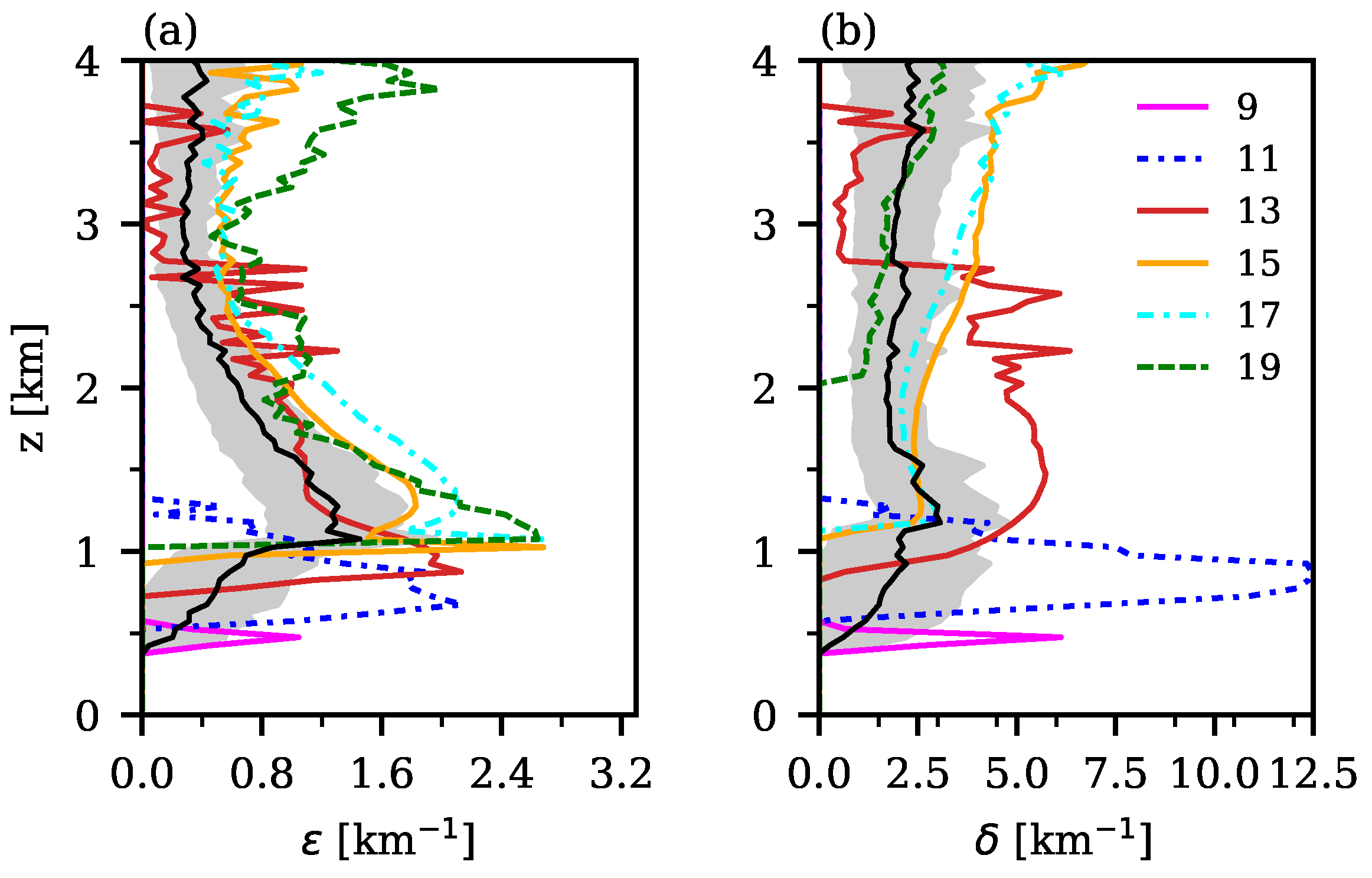
The fractional entrainment and detrainment rates for the ShCu composite case display pronounced diurnal variation. On average, and particularly during the maturity stage, the entrainment rate resembles that observed in the quasi-stationary BOMEX case, with maximum values near the cloud base (≈1.0 × 10⁻³ m⁻¹) and minimum values near the cloud top. However, the entrainment rate increases near the cloud top during the dissipation stage. The fractional detrainment rate, on the other hand, is nearly constant with the height on average (≈2.5 × 10⁻³ m⁻¹) but increases with the height during and after the maturity stage. This increase aligns with the findings from other LES studies conducted over both oceanic and continental environments. Overall, the detrainment rate consistently exceeds the entrainment rate, often by more than a factor of two.

(3)

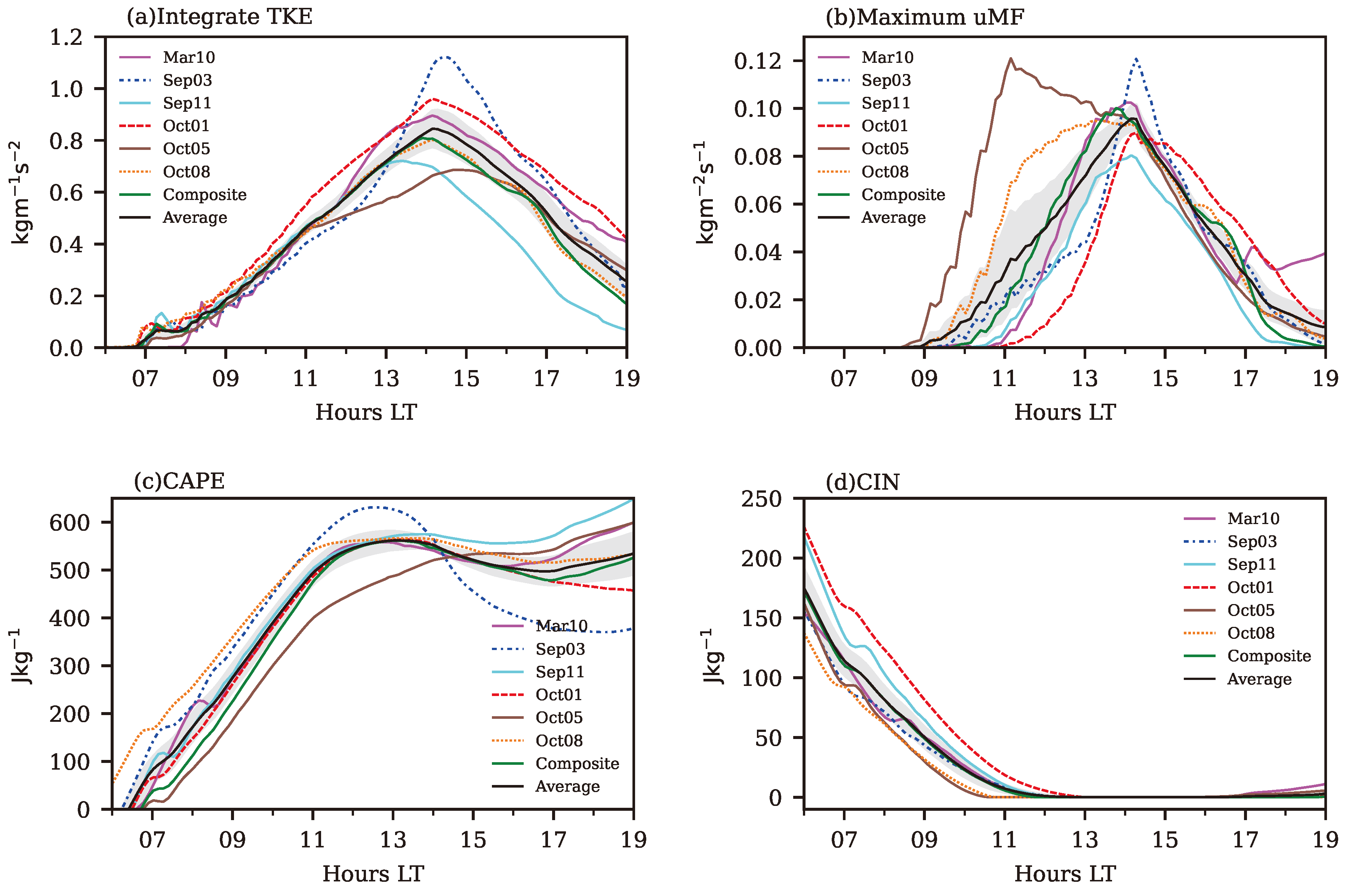
Relationship with atmospheric parameters: We analyzed the diurnal cycles of CAPE, CIN, BR, and the vertically integrated TKE in the mixed layer (ITKE-ML) and their relationships with the cloud base mass flux (Mb) and cloud depth for the six ShCu cases. The diurnal variations in the ITKE-ML and cloud base mass fluxes were similar, with peak values occurring around 14–15 LT. However, CAPE and BR did not show a clear relationship with Mb.

(4)

Cloud depth comparisons: Comparisons between the cloud depth and parameters such as CAPE, BR, ITKE-ML, CIN, and Mb did not reveal clear relationships. In some cases, higher CAPE and lower CIN values were observed for smaller ShCu clouds, or nearly similar BR values were found for both smaller and taller ShCu clouds.

(5)

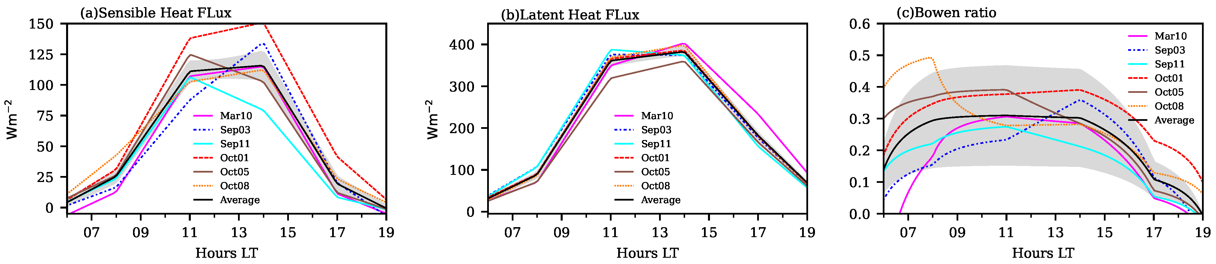
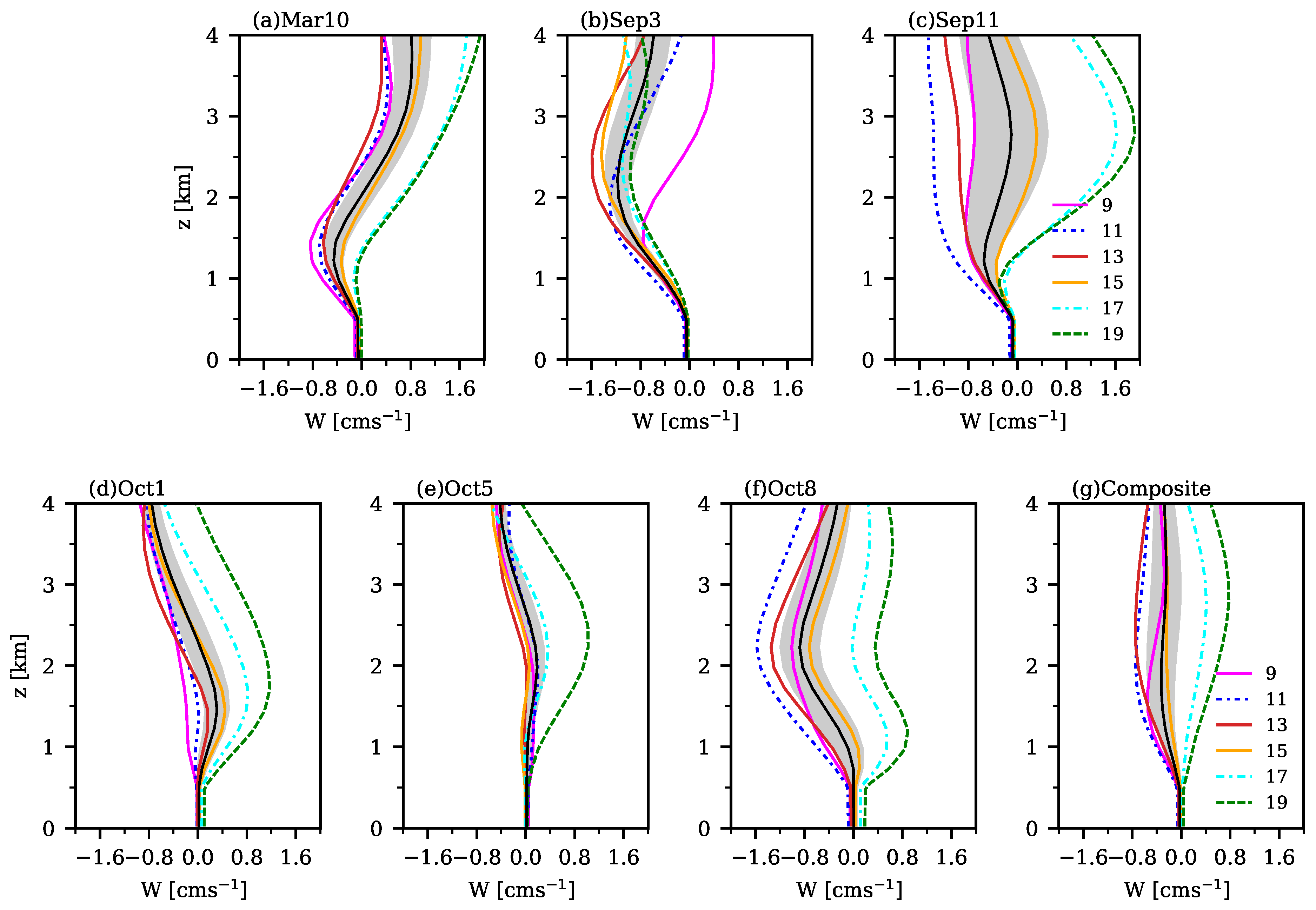
A significantly higher surface buoyancy flux is observed in the Sep3 case compared to Oct5. However, the cloud depths in these cases show the opposite trend, indicating that higher sensible or latent heat fluxes do not necessarily correspond to greater vertical cloud development. Our preliminary findings indicate that the vertical growth of ShCu clouds over the Central Amazon is more closely linked to enhanced buoyancy flux within the cloud layer and reduced large-scale subsidence than to surface fluxes.

These findings are preliminary, as they are based on a limited sample of six cases. Nonetheless, this study is the first to simulate the development of pure ShCu clouds over the Central Amazon. These results offer insights that could support the refinement of shallow cumulus parameterizations over land. However, further investigation, including a broader range of ShCu cases, is needed to validate these findings. The initial conditions and large-scale forcing for the composite ShCu is available (Data Availability Statement) to drive LES and single-column models. This composite represents a useful ShCu case over tropical land to evaluate ShCu parametrizations in numerical models.

References

1. Giangrande, S.E.; Feng, Z.; Jensen, M.P.; Comstock, J.M.; Johnson, K.L.; Toto, T.; Wang, M.; Burleyson, C.; Bharadwaj, N.; Mei, F.; et al. Cloud characteristics, thermodynamic controls and radiative impacts during the Observations and Modeling of the Green Ocean Amazon (GoAmazon2014/5) experiment. Atmos. Chem. Phys. 2017, 17, 14519–14541. [Google Scholar] [CrossRef]
2. Guichard, F.; Petch, J.; Redelsperger, J.L.; Bechtold, P.; Chaboureau, J.P.; Cheinet, S.; Grabowski, W.; Grenier, H.; Jones, C.; Köhler, M.; et al. Modelling the diurnal cycle of deep precipitating convection over land with cloud-resolving models and single-column models. Q. J. R. Meteorol. Soc. J. Atmos. Sci. Appl. Meteorol. Phys. Oceanogr. 2004, 130, 3139–3172. [Google Scholar] [CrossRef]
3. Zhang, Y.; Klein, S.A. Mechanisms Affecting the Transition from Shallow to Deep Convection over Land: Inferences from Observations of the Diurnal Cycle Collected at the ARM Southern Great Plains Site. J. Atmos. Sci. 2010, 67, 2943–2959. [Google Scholar] [CrossRef]
4. Waite, M.L.; Khouider, B. The deepening of tropical convection by congestus preconditioning. J. Atmos. Sci. 2010, 67, 2601–2615. [Google Scholar] [CrossRef]
5. Hohenegger, C.; Stevens, B. Preconditioning deep convection with cumulus congestus. J. Atmos. Sci. 2013, 70, 448–464. [Google Scholar] [CrossRef]
6. Kurowski, M.J.; Suselj, K.; Grabowski, W.W.; Teixeira, J. Shallow-to-deep transition of continental moist convection: Cold pools, surface fluxes, and mesoscale organization. J. Atmos. Sci. 2018, 75, 4071–4090. [Google Scholar] [CrossRef]
7. Fiedler, S.; Crueger, T.; D’Agostino, R.; Peters, K.; Becker, T.; Leutwyler, D.; Paccini, L.; Burdanowitz, J.; Buehler, S.A.; Cortes, A.U.; et al. Simulated Tropical Precipitation Assessed across Three Major Phases of the Coupled Model Intercomparison Project (CMIP). Mon. Weather Rev. 2020, 148, 3653–3680. [Google Scholar] [CrossRef]
8. Champouillon, A.; Rio, C.; Couvreux, F. Simulating the transition from shallow to deep convection across scales: The role of congestus clouds. J. Atmos. Sci. 2023, 80, 2989–3005. [Google Scholar] [CrossRef]
9. Vraciu, C.V.; Kruse, I.L.; Haerter, J.O. The role of passive cloud volumes in the transition from shallow to deep atmospheric convection. Geophys. Res. Lett. 2023, 50, e2023GL105996. [Google Scholar] [CrossRef]
10. Augstein, E.; Riehl, H.; Ostapoff, F.; Wagner, V. Mass and Energy Transports in an Undisturbed Atlantic Trade-Wind Flow. Mon. Weather Rev. 1973, 101, 101–111. [Google Scholar] [CrossRef]
11. Holland, J.Z.; Rasmusson, E.M. Measurements of the Atmospheric Mass, Energy, and Momentum Budgets Over a 500-Kilometer Square of Tropical Ocean. Mon. Weather Rev. 1973, 101, 44–55. [Google Scholar] [CrossRef]
12. Rauber, R.M.; Stevens, B.; Ochs, H.T.; Knight, C.; Albrecht, B.A.; Blyth, A.M.; Fairall, C.W.; Jensen, J.B.; Lasher-Trapp, S.G.; Mayol-Bracero, O.L.; et al. Rain in Shallow Cumulus Over the Ocean: The RICO Campaign. Bull. Am. Meteorol. Soc. 2007, 88, 1912–1928. [Google Scholar] [CrossRef]
13. Bony, S.; Stevens, B.; Ament, F.; Bigorre, S.; Chazette, P.; Crewell, S.; Delanoë, J.; Emanuel, K.; Farrell, D.; Flamant, C.; et al. EUREC 4 A: A field campaign to elucidate the couplings between clouds, convection and circulation. Surv. Geophys. 2017, 38, 1529–1568. [Google Scholar] [CrossRef] [PubMed]
14. Zhang, Y.; Klein, S.A.; Fan, J.; Chandra, A.S.; Kollias, P.; Xie, S.; Tang, S. Large-eddy simulation of shallow cumulus over land: A composite case based on ARM long-term observations at its Southern Great Plains site. J. Atmos. Sci. 2017, 74, 3229–3251. [Google Scholar] [CrossRef]
15. Vogelmann, A.M.; McFarquhar, G.M.; Ogren, J.A.; Turner, D.D.; Comstock, J.M.; Feingold, G.; Long, C.N.; Jonsson, H.H.; Bucholtz, A.; Collins, D.R.; et al. RACORO extended-term aircraft observations of boundary layer clouds. Bull. Am. Meteorol. Soc. 2012, 93, 861–878. [Google Scholar] [CrossRef]
16. Martin, S.T.; Artaxo, P.; Machado, L.A.T.; Manzi, A.O.; Souza, R.A.F.; Schumacher, C.; Wang, J.; Andreae, M.O.; Barbosa, H.M.J.; Fan, J.; et al. Introduction: Observations and Modeling of the Green Ocean Amazon (GoAmazon 2014/5). Atmos. Chem. Phys. 2016, 16, 4785–4797. [Google Scholar] [CrossRef]
17. Betts, A.K. Non-precipitating cumulus convection and its parameterization. Q. J. R. Meteorol. Soc. 1973, 99, 178–196. [Google Scholar]
18. Tiedtke, M.; Heckley, W.; Slingo, J. Tropical forecasting at ECMWF: The influence of physical parametrization on the mean structure of forecasts and analyses. Q. J. R. Meteorol. Soc. 1988, 114, 639–664. [Google Scholar] [CrossRef]
19. Siebesma, A.P.; Cuijpers, J.W.M. Evaluation of Parametric Assumptions for Shallow Cumulus Convection. J. Atmos. Sci. 1995, 52, 650–666. [Google Scholar] [CrossRef]
20. Siebesma, A.P.; Holtslag, A.A.M. Model impacts of entrainment and detrainment rates in shallow cumulus convection. J. Atmos. Sci. 1996, 53. [Google Scholar] [CrossRef]
21. Grant, A.L.M.; Brown, A.R. A similarity hypothesis for shallow-cumulus transports. Q. J. R. Meteorol. Soc. 1999, 125, 1913–1936. [Google Scholar] [CrossRef]
22. Neggers, R.A.J.; Neelin, J.D.; Stevens, B. Impact Mechanisms of Shallow Cumulus Convection on Tropical Climate Dynamics. J. Clim. 2007, 20, 2623–2642. [Google Scholar] [CrossRef]
23. Zheng, Y. Theoretical Understanding of the Linear Relationship between Convective Updrafts and Cloud-Base Height for Shallow Cumulus Clouds. Part I: Maritime Conditions. J. Atmos. Sci. 2019, 76, 2539–2558. [Google Scholar] [CrossRef]
24. Tang, S.; Xie, S.; Guo, Z.; Hong, S.Y.; Khouider, B.; Klocke, D.; Köhler, M.; Koo, M.S.; Krishna, P.M.; Larson, V.E.; et al. Long-term single-column model intercomparison of diurnal cycle of precipitation over midlatitude and tropical land. Q. J. R. Meteorol. Soc. 2021, 148, 641–669. [Google Scholar] [CrossRef]
25. Tian, Y.; Zhang, Y.; Klein, S.A.; Schumacher, C. Interpreting the diurnal cycle of clouds and precipitation in the ARM GoAmazon observations: Shallow to deep convection transition. J. Geophys. Res. Atmos. 2021, 126, e2020JD033766. [Google Scholar] [CrossRef]
26. Grabowski, W.; Bechtold, P.; Cheng, A.; Forbes, R.; Halliwell, C.; Khairoutdinov, M.; Lang, S.; Nasuno, T.; Petch, J.; Tao, W.K.; et al. Daytime convective development over land: A model intercomparison based on LBA observations. Q. J. R. Meteorol. Soc. J. Atmos. Sci. Appl. Meteorol. Phys. Oceanogr. 2006, 132, 317–344. [Google Scholar] [CrossRef]
27. Khairoutdinov, M.; Randall, D. High-resolution simulation of shallow-to-deep convection transition over land. J. Atmos. Sci. 2006, 63, 3421–3436. [Google Scholar] [CrossRef]
28. Efstathiou, G.A. Dynamic subgrid turbulence modeling for shallow cumulus convection simulations beyond LES resolutions. J. Atmos. Sci. 2023, 80, 1519–1545. [Google Scholar] [CrossRef]
29. Efstathiou, G.A.; Plant, R.S.; Chow, F.K. Grey-zone simulations of shallow-to-deep convection transition using dynamic subgrid-scale turbulence models. Q. J. R. Meteorol. Soc. 2024, 150, 4306–4328. [Google Scholar] [CrossRef]
30. Tang, S.; Xie, S.; Zhang, Y.; Zhang, M.; Schumacher, C.; Upton, H.; Jensen, M.P.; Johnson, K.L.; Wang, M.; Ahlgrimm, M.; et al. Large-scale vertical velocity, diabatic heating and drying profiles associated with seasonal and diurnal variations of convective systems observed in the GoAmazon 2014/5 experiment. Atmos. Chem. Phys. 2016, 16, 14249–14264. [Google Scholar] [CrossRef]
31. Grabowski, W.W. Daytime convective development over land: The role of surface forcing. Q. J. R. Meteorol. Soc. 2023, 149, 2800–2819. [Google Scholar] [CrossRef]
32. Siebesma, A.P.; Bretherton, C.S.; Brown, A.; Chlond, A.; Cuxart, J.; Duynkerke, P.G.; Jiang, H.; Khairoutdinov, M.; Lewellen, D.; Moeng, C.H.; et al. A large eddy simulation intercomparison study of shallow cumulus convection. J. Atmos. Sci. 2003, 60, 1201–1219. [Google Scholar] [CrossRef]
33. Brown, A.R.; Cederwall, R.T.; Chlond, A.; Duynkerke, P.G.; Golaz, J.C.; Khairoutdinov, M.; Lewellen, D.C.; Lock, A.P.; MacVean, M.K.; Moeng, C.H.; et al. Large-eddy simulation of the diurnal cycle of shallow cumulus convection over land. Q. J. R. Meteorol. Soc. 2002, 128, 1075–1093. [Google Scholar] [CrossRef]
34. Neggers, R.A.J.; Duynkerke, P.G.; Rodts, S.M.A. Shallow cumulus convection: A validation of large-eddy simulation against aircraft and Landsat observations. Q. J. R. Meteorol. Soc. J. Atmos. Sci. Appl. Meteorol. Phys. Oceanogr. 2003, 129, 2671–2696. [Google Scholar] [CrossRef]
35. Grant, A.L.M. The cumulus-capped boundary layer. I: Modelling transports in the cloud layer. Q. J. R. Meteorol. Soc. 2006, 132, 1385–1403. [Google Scholar] [CrossRef]
36. Neggers, R.A.J. Exploring bin-macrophysics models for moist convective transport and clouds. J. Adv. Model. Earth Syst. 2015, 7, 2079–2104. [Google Scholar] [CrossRef]
37. Song, F.; Zhang, G.J. Improving Trigger Functions for Convective Parameterization Schemes Using GOAmazon Observations. J. Clim. 2017, 30, 8711–8726. [Google Scholar] [CrossRef]
38. Lamaakel, O.; Matheou, G. Galilean invariance of shallow cumulus convection large-eddy simulations. J. Comput. Phys. 2021, 427, 110012. [Google Scholar] [CrossRef]
39. Khairoutdinov, M.F.; Randall, D.A. Cloud Resolving Modeling of the ARM Summer 1997 IOP: Model Formulation, Results, Uncertainties, and Sensitivities. J. Atmos. Sci. 2003, 60, 607–625. [Google Scholar] [CrossRef]
40. Smagorinsky, J. General circulation experiments with the primitive equations: I. The basic experiment. Mon. Weather Rev. 1963, 91, 99–164. [Google Scholar] [CrossRef]
41. Collins, W.D.; Bitz, C.M.; Blackmon, M.L.; Bonan, G.B.; Bretherton, C.S.; Carton, J.A.; Chang, P.; Doney, S.C.; Hack, J.J.; Henderson, T.B.; et al. The community climate system model version 3 (CCSM3). J. Clim. 2006, 19, 2122–2143. [Google Scholar] [CrossRef]
42. Nuijens, L.; Stevens, B.; Siebesma, A.P. The environment of precipitating shallow cumulus convection. J. Atmos. Sci. 2009, 66, 1962–1979. [Google Scholar] [CrossRef]
43. Arulraj, M.; Barros, A.P. Shallow Precipitation Detection and Classification Using Multifrequency Radar Observations and Model Simulations. J. Atmos. Ocean. Technol. 2017, 34, 1963–1983. [Google Scholar] [CrossRef]
44. Fu, Y.; Chen, Y.; Zhang, X.; Wang, Y.; Li, R.; Liu, Q.; Zhong, L.; Zhang, Q.; Zhang, A. Fundamental characteristics of tropical rain cell structures as measured by TRMM PR. J. Meteorol. Res. 2020, 34, 1129–1150. [Google Scholar] [CrossRef]
45. Collow, A.B.M.; Miller, M.A. The seasonal cycle of the radiation budget and cloud radiative effect in the Amazon rain forest of Brazil. J. Clim. 2016, 29, 7703–7722. [Google Scholar] [CrossRef]
46. Arakawa, A.; Schubert, W.H. Interaction of a Cumulus Cloud Ensemble with the Large-Scale Environment, Part I. J. Atmos. Sci. 1974, 31, 674–701. [Google Scholar] [CrossRef]
47. Lamer, K.; Kollias, P.; Nuijens, L. Observations of the variability of shallow trade wind cumulus cloudiness and mass flux. J. Geophys. Res. Atmos. 2015, 120, 6161–6178. [Google Scholar] [CrossRef]
48. Sakradzija, M.; Hohenegger, C. What determines the distribution of shallow convective mass flux through a cloud base? J. Atmos. Sci. 2017, 74, 2615–2632. [Google Scholar] [CrossRef]
49. Klingebiel, M.; Konow, H.; Stevens, B. Measuring shallow convective mass flux profiles in the trade wind region. J. Atmos. Sci. 2021, 78, 3205–3214. [Google Scholar] [CrossRef]
50. Kumar, V.V.; Jakob, C.; Protat, A.; Williams, C.R.; May, P.T. Mass-flux characteristics of tropical cumulus clouds from wind profiler observations at Darwin, Australia. J. Atmos. Sci. 2015, 72, 1837–1855. [Google Scholar] [CrossRef]
51. Masunaga, H.; Luo, Z.J. Convective and large-scale mass flux profiles over tropical oceans determined from synergistic analysis of a suite of satellite observations. J. Geophys. Res. Atmos. 2016, 121, 7958–7974. [Google Scholar] [CrossRef] [PubMed]
52. George, G.; Stevens, B.; Bony, S.; Klingebiel, M.; Vogel, R. Observed impact of meso-scale vertical motion on cloudiness. J. Atmos. Sci. 2021, 78, 2413–2427. [Google Scholar] [CrossRef]
53. Jeyaratnam, J.; Luo, Z.J.; Giangrande, S.E.; Wang, D.; Masunaga, H. A Satellite-Based Estimate of Convective Vertical Velocity and Convective Mass Flux: Global Survey and Comparison with Radar Wind Profiler Observations. Geophys. Res. Lett. 2021, 48, e2020GL090675. [Google Scholar] [CrossRef]
54. Grant, A.L.M. Cloud-base fluxes in the cumulus-capped boundary layer. Q. J. R. Meteorol. Soc. 2001, 127, 407–421. [Google Scholar]
55. Wang, X.; Zhang, M. Vertical velocity in shallow convection for different plume types. J. Adv. Model. Earth Syst. 2014, 6, 478–489. [Google Scholar] [CrossRef]
56. Drueke, S.; Kirshbaum, D.J.; Kollias, P. Environmental sensitivities of shallow-cumulus dilution–Part 1: Selected thermodynamic conditions. Atmos. Chem. Phys. 2020, 20, 13217–13239. [Google Scholar] [CrossRef]
57. Oh, G.; Austin, P.H. Direct Entrainment as a Measure of Dilution. J. Atmos. Sci. 2024, 81, 1783–1797. [Google Scholar] [CrossRef]
58. De Rooy, W.C.; Siebesma, A.P. A simple parameterization for detrainment in shallow cumulus. Mon. Weather. Rev. 2008, 136, 560–576. [Google Scholar] [CrossRef]
59. Lu, C.; Liu, Y.; Zhang, G.J.; Wu, X.; Endo, S.; Cao, L.; Li, Y.; Guo, X. Improving parameterization of entrainment rate for shallow convection with aircraft measurements and large-eddy simulation. J. Atmos. Sci. 2016, 73, 761–773. [Google Scholar] [CrossRef]
60. Bretherton, C.S.; McCaa, J.R.; Grenier, H. A new parameterization for shallow cumulus convection and its application to marine subtropical cloud-topped boundary layers. Part I: Description and 1D results. Mon. Weather Rev. 2004, 132, 864–882. [Google Scholar] [CrossRef]
61. Shin, J.; Baik, J.J. Parameterization of stochastically entraining convection using machine learning technique. J. Adv. Model. Earth Syst. 2022, 14, e2021MS002817. [Google Scholar] [CrossRef]
62. Bechtold, P.; Cuijpers, J.W. Cloud perturbations of temperature and humidity: A LES study. Bound. Layer Meteorol. 1995, 76, 377–386. [Google Scholar] [CrossRef]
63. Grant, A.L.M.; Lock, A.P. The turbulent kinetic energy budget for shallow cumulus convection. Q. J. R. Meteorol. Soc. 2004, 130, 401–422. [Google Scholar] [CrossRef]
64. Cuijpers, J.; Duynkerke, P. Large eddy simulation of trade wind cumulus clouds. J. Atmos. Sci. 1993, 50, 3894–3908. [Google Scholar] [CrossRef]
65. Zheng, Y.; Rosenfeld, D. Linear relation between convective cloud base height and updrafts and application to satellite retrievals. Geophys. Res. Lett. 2015, 42, 6485–6491. [Google Scholar] [CrossRef]
66. Zheng, Y.; Rosenfeld, D.; Li, Z. Sub-Cloud Turbulence Explains Cloud-Base Updrafts for Shallow Cumulus Ensembles: First Observational Evidence. Geophys. Res. Lett. 2021, 48, e2020GL091881. [Google Scholar] [CrossRef]
67. Raymond, D.; Fuchs-Stone, Z. Weak Temperature Gradient Modeling of Convection in OTREC. J. Adv. Model. Earth Syst. 2021, 13. [Google Scholar] [CrossRef]
68. Becker, T.; Bechtold, P.; Sandu, I. Characteristics of convective precipitation over tropical Africa in storm-resolving global simulations. Q. J. R. Meteorol. Soc. 2021, 147, 4388–4407. [Google Scholar] [CrossRef]
69. Mapes, B.E. Convective inhibition, subgrid-scale triggering energy, and stratiform instability in a toy tropical wave model. J. Atmos. Sci. 2000, 57, 1515–1535. [Google Scholar] [CrossRef]
70. Kuang, Z.; Bretherton, C.S. A mass-flux scheme view of a high-resolution simulation of a transition from shallow to deep cumulus convection. J. Atmos. Sci. 2006, 63, 1895–1909. [Google Scholar] [CrossRef]
71. Park, S.; Bretherton, C.S. The University of Washington shallow convection and moist turbulence schemes and their impact on climate simulations with the Community Atmosphere Model. J. Clim. 2009, 22, 3449–3469. [Google Scholar] [CrossRef]
Figure 1. (Left)Locations of the experimental sites ARM and SIPAM (at Ponta Pelada airport, near Manaus) and the variational analysis domain (green octagon) centered at the SIPAM site, with a 110 km radius [30]. This green octagonal region, covering approximately 2° × 2° in latitude and longitude, is called the Central Amazon (CAMZ). (Right): (a) Illustrative cloud-type classification by Giangrande et al. [1] for the 10 March 2014 event at the ARM site, showing the diurnal cycle of shallow cumulus (ShCu). Daily precipitation for March (b), and for September and October (c), averaged over the CAMZ using the Tang et al. [30] product for the GoAmazon-2014 campaigns during the intensive operational periods IOP1 (February–March) and IOP2 (September–October).
Atmosphere 16 00789 g001
Figure 2. Observed cloud mask and its time evolution (hours in LT) for 9 selected days in the intensive operational period over the GoAmazon campaign through 2014, showing the presence of pure shallow cumulus.
Atmosphere 16 00789 g002
Figure 3. Initial conditions and large-scale forcing profiles for the shallow cumulus (ShCu) composite, including (a) potential temperature and total specific humidity, (b) zonal and meridional wind velocities, (c) vertical velocity, (d) horizontal advection of temperature, and (e) specific humidity. The ShCu composite was derived by averaging the initial conditions and large-scale forcings from the six ShCu cases depicted in Figure 2.
Atmosphere 16 00789 g003
Figure 4. Diurnal cycles of (a) sensible heat flux, (b) latent heat flux, and (c) Bowen ratio for six ShCu cases, with the average profiles (black line) and ±0.5 standard deviation (grey shaded area).
Atmosphere 16 00789 g004
Figure 5. Diurnal cycle of the cloud fraction (a) and liquid water content (b) profiles for the composite ShCu case.
Atmosphere 16 00789 g005
Figure 6. Diurnal cycle of the cloud fraction (CF) from 9 to 19 LT, represented with different lines and colors, for the six selected ShCu cases (af) and the composite ShCu (g). The gray shaded area indicates ±0.5 standard deviation and the black line the average profile.
Atmosphere 16 00789 g006
Figure 7. As in Figure 6 but for liquid water (LW) profiles.
Atmosphere 16 00789 g007
Figure 8. Similar to Figure 6 but for the updraft mass flux (uMF) profiles.
Atmosphere 16 00789 g008
Figure 9. As in Figure 6 but for the buoyancy flux (B).
Atmosphere 16 00789 g009
Figure 10. Schematic representation of a shallow cumulus cloud (light blue) simulated at 15 LT (orange line) for the ShCu composite case. The figure includes the cloud fraction profiles (panel a) and buoyancy flux (panel b). Th key terms include uMF (updraft mass flux), LCL (lifting condensation level), LFC (level of free convection), Shb (shallow cloud base height), and Shtop (cloud top height). E and D denote the entrainment and detrainment processes, respectively.
Atmosphere 16 00789 g010
Figure 11. Diurnal cycle of the fractional entrainment rate ϵ (a) and fractional detrainment rate δ (b), both expressed in km−1, from 9 to 19 LT. Different lines and colors represent the composite ShCu case depicted in Figure 5, while the black line indicates the average over the entire simulation period.
Atmosphere 16 00789 g011
Figure 12. As in Figure 6, but for the liquid water potential temperature flux.
Atmosphere 16 00789 g012
Figure 13. As in Figure 6, but for the total water flux.
Atmosphere 16 00789 g013
Figure 14. As in Figure 6 but for the vertical observed velocity w profiles.
Atmosphere 16 00789 g014
Figure 15. As in Figure 6, but for the turbulent kinetic energy (TKE).
Atmosphere 16 00789 g015
Figure 16. Diurnal cycle of the vertically integrated TKE in the ML (ITKE-ML) (a), cloud base mass flux (Mb) (b), convective available potential energy (CAPE) (c), and convective inhibition (CIN) (d).
Atmosphere 16 00789 g016
Disclaimer/Publisher’s Note: The statements, opinions and data contained in all publications are solely those of the individual author(s) and contributor(s) and not of MDPI and/or the editor(s). MDPI and/or the editor(s) disclaim responsibility for any injury to people or property resulting from any ideas, methods, instructions or products referred to in the content.