Review

An Audiovisual Introduction to Streamer Physics

Department for Space Research and Technology (DTU Space), Technical University of Denmark, Elektrovej 348, 2800 Kongens Lyngby, Denmark
Atmosphere 2025, 16(7), 757; https://doi.org/10.3390/atmos16070757
Submission received: 18 March 2025 / Revised: 11 June 2025 / Accepted: 16 June 2025 / Published: 20 June 2025

Abstract

Streamers are small, thin plasma channels that form the precursors of hot lightning leaders and that are associated with phenomena such as transient luminous events or terrestrial gamma-ray flashes. We provide an easily accessible audiovisual introduction for students and early researchers, serving as a supplement to traditional review papers. This overview contains an introduction to the collision-dominated motion of electrons in an ambient field and an ambient gas, including a discussion of cross-sections and friction force. Based on this, we will discuss electron avalanches before moving to streamers. Here, we will focus on the avalanche-to-streamer transition and present properties and different modeling approaches. Finally, we will discuss streamers in different gas mixtures as well as their relation to lightning and plasma chemistry. The viewer of the supplementary video will receive a first overview of streamer physics.

1. Introduction

Streamers are thin, small (at standard temperature and pressure, i.e., at a temperature of 300 K and a pressure of 1 bar) and cold plasma channels that form the precursors of long, hot lightning leaders [1,2,3,4,5], appear as transient luminous events (TLEs) above thunderclouds [6,7,8,9] and play a crucial role in plasma technology, such as in combustion [10,11], plasma medicine [12,13] or switch technology [14,15,16,17,18]. Streamers occur in different polarities with different propagation mechanisms [19,20,21,22] and are associated with the emission of energetic X-rays in laboratory discharges [23,24,25,26,27,28] as well as of terrestrial gamma-ray flashes (TGFs) in thunderstorms [29,30,31,32,33,34]. Although the majority of research in discharge physics concerns streamers in air, more and more research is performed regarding streamers in non-terrestrial gas mixtures such as N2:CH4 (as on Saturn’s moon Titan) [35], in Jovian and Venusian atmospheres [36], for Primordial Earth [37] or in air with admixtures of methane used for combustion [38].
There are plenty of books and review papers [1,39,40,41,42] addressing the physics, modeling and laboratory experiments of streamers. However, for new students and researchers, the available material might be overwhelming and it might be difficult in the beginning to sort out the relevant information. Additionally, it cannot be assumed that those universities and research institutes that research atmospheric electricity or plasma physics, including the investigation of streamers, offer courses covering streamer physics on an undergraduate level. Subsequently, it will take a significant amount of time for students to dive into the field of discharge physics, which is missing from the actual student or research project. Thus, we are concerned about how to provide easy access to this vivid research topic.
Additionally, previous research has shown that the attention span of an average human is in the order of tens of seconds up to tens of minutes [43,44,45] and also that the brains of different people work in different ways; for some, it is easier to process information visually while others have an advantage in processing data in an audio manner. Thus, we here present audiovisual access to streamer physics, which can be regarded as easy access and a supplement to more sophisticated literature on discharge physics. Finally, in recent decades, public outreach has become more and more important for the scientific communities [46,47], see [48] for an example of how lightning in the atmosphere of Primordial Earth was made more accessible to a broader audience. Although the present audiovisual review is tailored to the academic community, it might give concepts of how to present discharge physics to the public.

2. Conceptualization and Structure of This Introduction

The idea of such a review originated from a Zoom meeting in 2020 where we presented an introduction to streamer physics to the scientists at the St. Andrews Centre for Exoplanet Science [49] in Scotland, working on exoplanets and needing insight into lightning physics. In order to conserve the provided information for later use and check, this Zoom call was recorded. In the following years, we used this video as an introduction for students working on various projects of discharge physics. This raised the idea of publishing such an audiovisual introduction for the scientific community.
The video is provided as Supplementary Materials and covers the following topics:
  • collision-dominated electron motion in gases, cross-sections
  • electron avalanches
  • streamer discharges (avalanche-to-streamer transition, properties, modeling, streamers in other atmospheres)
  • relation to lightning and chemistry
Copyright details are provided in Table A1.

3. Contents of the Video: From Electron Avalanches to Streamer Discharges

The Supplement Video provides an in-depth introduction to electron avalanches and streamer physics, focusing on the avalanche-to-streamer transition as well as the physics, properties, and occurrences of streamers. The video covers various aspects, including technological applications, the nature of streamers, and their relation to lightning and plasma chemistry, which will be summarized in the following subsections.

3.1. Introduction to Streamers (Slide 3)

Streamers occur both in nature as well as in applications and experiments. The most common occurrence is probably in lightning [50], which is mediated and facilitated by streamer discharges. Hence, if streamers are absent in a given atmospheric gas composition, then lightning cannot appear. Above thunderstorms, transient luminous events (TLEs) [6] partly or fully consist of streamers. They can also occur in technological or experimental setups. Applying a voltage between two electrodes (e.g., a needle and a plate electrode) [51] will trigger a discharge which, under some circumstances (see Section 3.3) will be a streamer discharge. Streamers can be used for combustion [38], switching applications [52], or plasma medicine allowing the treatment of wounds.

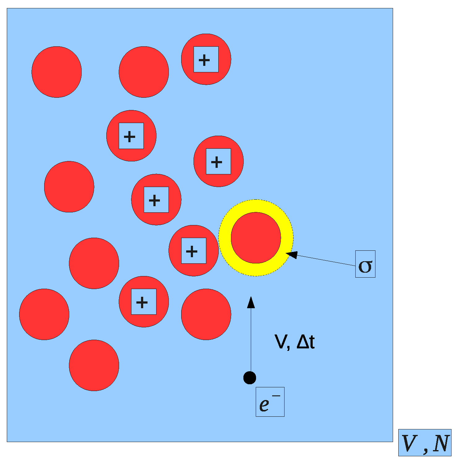
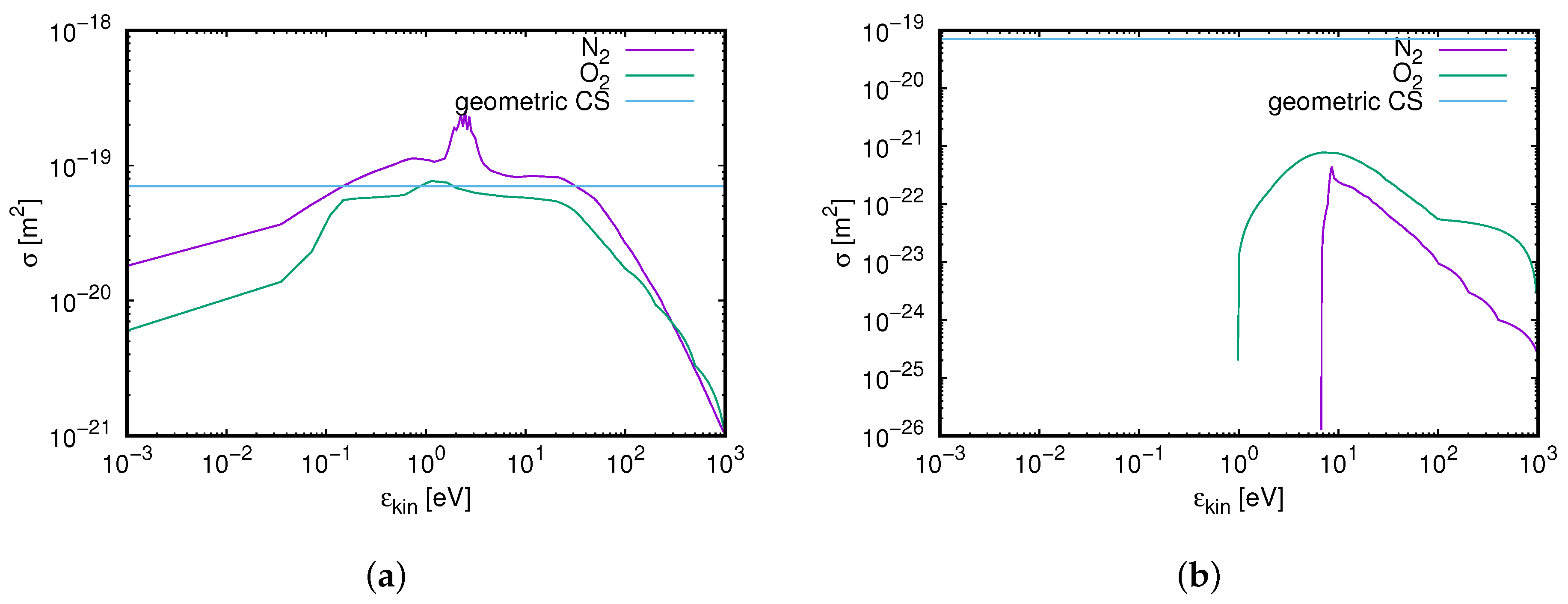
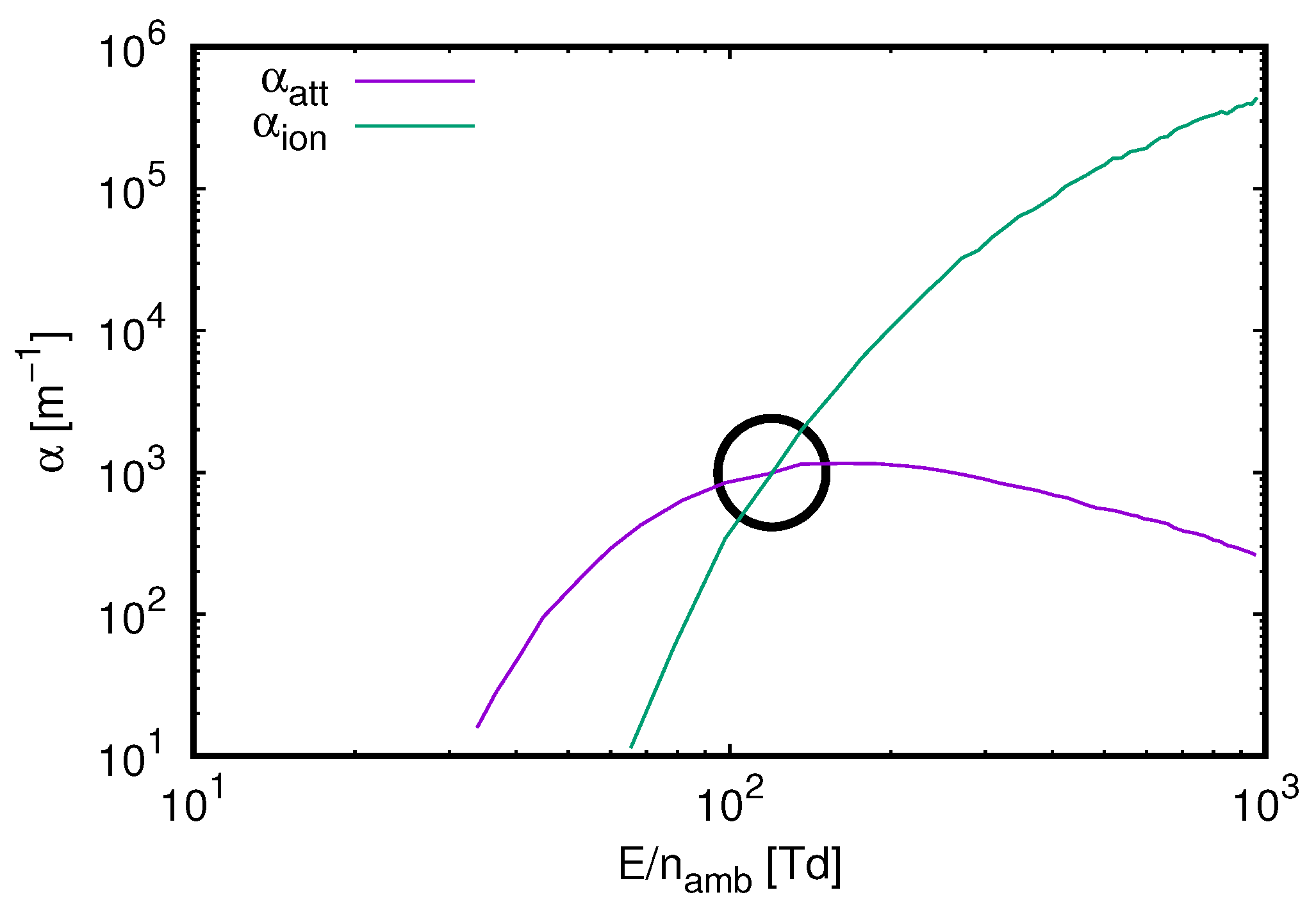
3.2. Fundamentals of Electron Motion in Gases (Slides 4–8)

The physics of streamers really is determined by the collective motion of individual electrons in an ambient gas; see Figure 1 for the general setup. Let us assume that we have two electrodes. If there were no gas in between, electrons would accelerate in the ambient field generated by the two electrons, and we could simply apply the laws of electrodynamics to describe the motion of the electrons. This picture changes completely when we consider an ambient gas between the electrodes since the electrons will then interact with the gas molecules. There are different collision channels, such as elastic scattering, and when electrons have reached sufficiently high threshold energies, excitations, as well as electron impact ionization, liberate new electrons from the orbitals of the ambient gas species, thus leading to electron multiplication. While elastic scattering mostly conserves the electron energies, electrons lose energy through excitations and ionization; hence, there is a balance between energy gain through the ambient electric field and energy loss through collisions. In the following, let us consider air (consisting of 80% molecular nitrogen N 2 and 20% molecular oxygen O 2 ) at standard temperature and pressure (300 K and 1 bar), but the general concepts can, of course, be applied to other mixtures.
The scattering probability within a time step Δ t (see Section 3.5 for details of the time stepping) is given by
P = 1 e n a m b v ( ϵ ) Δ t σ t o t ( ϵ )
where n a m b is the ambient gas density, v is the electron velocity, depending on the electron energy ϵ , and σ t o t ( ϵ ) is the total collision cross-section, which is the sum over all cross-section σ i , j of all considered processes. With the help of the cross-section, we then can also define the effective friction force of electrons in an ambient gas as [3]
F = i , j n i σ i , j ( ϵ ) Δ ϵ i , j
where i indices the species of the gas mixture and j is the index of the actual collision process (e.g., elastic scattering) per species i. n i is the partial density of species i [ m 3 ], Δ ϵ i , j is the average energy loss electrons through the collision process j at gas species i, and σ i , j ( ϵ ) is the corresponding cross-section of collision process j of electron scattering off gas species i.
In the classical, non-quantum interpretation, the cross-section σ can be considered the interaction area
σ = π ( r 1 + r 2 ) 2
of two colliding bodies with radii r 1 and r 2 (Figure 2). For example, if we use the classical electron radius r e , c l a s s = 2.8179 × 10 15 m and the van-der-Waals radius r N 2 , v a n d e r W a a l s = 155 × 10 12 m for molecular nitrogen, the cross-section for electron scattering off N 2 is approximately σ 7 × 10 20 m 2 . However, this definition is problematic as electrons and gas molecules are quantum particles. Hence, we cannot define a fixed radius for the interacting particles. Additionally, we cannot use such a geometric approach, but need to consider the scattering as a quantum process, where we have to consider electrons before scattering as a free wave, which is modified at the collision center (the molecule). Hence, cross-sections depend on the kinetic energy of electrons. As an example, Figure 3a shows the cross-section of the elastic scattering of electrons from air molecules [53]. It shows that the order of magnitude is indeed ≈ 7 × 10 20 m 2 , but that the cross-section actually depends on the electron energy, including resonances. Panel (b) shows an example of an excitation channel [53]. As aforementioned, excitations and ionization collisions require a minimum electron threshold energy. Hence, such cross-sections are only valid for larger energies.
Starting with the collision probability (1), we can define the mean free path, which is the average distance an electron travels between two collisions, as
Λ M F P = n a m b σ t o t ( ϵ ) 1
and rewrite Equation (1) as
P = 1 e Δ z Λ M F P
where Δ z = v Δ t is the travelled distance during time step Δ t . This allows us to derive some fundamental scaling laws about the electron motion and collisions in a gas. Equation (5) indicates that the collision probability scales with the inverse of the mean free path (4), which in turn depends on the ambient density. Therefore, typical length scales of the collision-dominated electron motion scale with Δ z n a m b 1 . The electron energies depend on the energy threshold energies of the excited states of the gas molecules as well as on the ionization energies, hence ϵ n a m b 0 . As the velocities depend on the electron energy, it is v n a m b 0 and thus Δ t n a m b 1 for typical time scales. Now, the applied voltage in a laboratory discharge or the available voltage in a thundercloud does not depend on the ambient gas density, but since the electric field is defined as voltage (or potential) per length, it scales with ∼ n a m b which motivates the definition of the reduced electric field.
E n a m b [ T d = 10 21 V m 2 ] .
This basically means that the physics of the electron motion is unaltered when you scale the ambient field and the ambient density by the same factor, with the exception that time and length scales are proportional to n a m b 1 .
Figure 4 shows the friction force (2) for electrons in air [3,54]. The friction force determines the electron motion in air. If the friction is zero, i.e., if there is no ambient gas, the motion is purely determined through the Lorentz force
d p d t = q E
where q is the electron charge. If there is an ambient gas and thus a friction force F , this equation changes to
d p d t = q E F ( ϵ , r ) ,
in principle allowing the analytic or numerical calculation of the average motion of an electron in a gas. However, this is a very simplified approach and only valid for the average motion since the friction force depends on the cross-sections (2), which—as aforementioned—reflects the quantum nature of electrons at air molecules. Hence, Equation (8) does not take into account the randomness of the electron–molecule collisions. Note that the force F and the electric field E are equivalent and only differ by a factor e 0 1.602 × 10 19 which is the elementary charge allowing the relating of the friction force to the electric field strength or vice versa. If | e 0 E | | F | , then there is a net acceleration/deceleration; if | e 0 E | = | F | , electrons have reached an equilibrium point where their energy is conserved. As an example, let us apply a field of E k = 3.2 MV m 1 , which is the breakdown field at standard temperature and pressure in air (see Section 3.3), and let us start with electrons with an initial energy of ≈1 eV. Although there are electron–molecule collisions (with their quantum nature), there is a net acceleration, and electrons gain sufficient energies to excite or ionize air molecules. Although some of the electrons lose some of their energy, there is an overall acceleration. At approximately 20 eV, the electric force and the friction force reach an equilibrium point (indicated by the green lines), limiting the electron energy. Because of the random nature of collisions, some electrons might not collide and gain more energy. However, in this case, the friction force becomes larger than the electric force, decelerating electrons down to the equilibrium point. The maximum of the friction force in air occurs at approx. 100–200 eV, and one needs electric fields on the order of 8–9 E k to overcome this friction barrier; for larger energies, the friction decreases. This is what we call the runaway regime where electrons keep being accelerated systematically while their acceleration to higher energies is rather stochastic due to the quantum nature of collisions. Such electrons can almost reach the speed of light and are connected to high-energy phenomena, which is out of the scope of this paper.

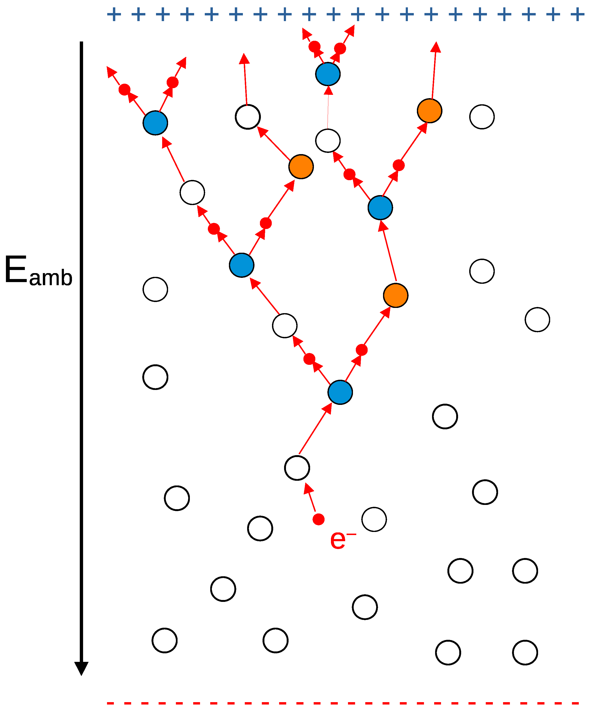
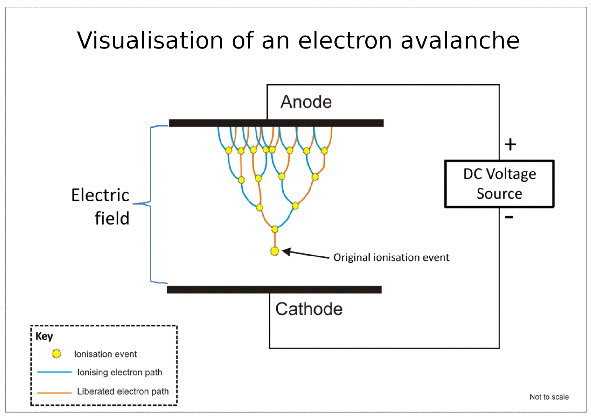
3.3. Electron Avalanches and the Avalanche-to-Streamer Transition (Slides 9–13)

The first step towards a streamer discharge is an electron avalanche formed through electron impact ionization in the electric field of two electrodes (Figure 5). For a given electron number N e moving towards the anode, the number d N e of new electrons within a distance d x is
d N e = N e α i o n α a t t d x
where α i o n is the ionization coefficient, and α a t t is the attachment coefficient for electrons attaching to molecules yielding a negative ion, both depending on the local electric field. The solution of Equation (9), determining the electron number N e ( x ) at position x, is
N e ( x ) = N e , 0 e ( α i o n α a t t ) x
where N e , 0 is the initial electron number. This is what we refer to as an electron avalanche.
After producing electron-ion pairs, electrons typically separate from the ions due to their lighter mass and create so-called space charge effects [1]. The corresponding space charge electric field is determined through
· E s p a c e = e 0 n + n ϵ 0
where n + is the density of positive ions, n is the density of negative charges (ions and electrons), and where ϵ 0 8.85 × 10 12 A s (V m)−1 is the vacuum permittivity. The avalanche turns into a streamer when
E s p a c e E a m b .
Under this condition, there is a local amplification of the electric field, energizing electrons further yielding additional ionization. This is the self-sustained streamer discharge with its accelerated growth of the electron number as well as electrons reaching energies sufficiently high to excite ambient gas molecules to states where they can emit visible photons. The Raether-Meek criterion [56,57] states that the condition (12) is typically obtained after 18–20 avalanche processes, i.e., ( α i o n α a t t ) d 18–20, or equivalently after creating
e ( α i o n α a t t ) d 10 8 10 9
electrons in air in the absence of any electrodes or other conductive material. However, the number of 18–20 avalanche processes really depends on the gas mixture of the effect of electrodes or hydrometeors, see [58,59].
As Equation (10) indicates, the growth of electron avalanches and streamers depends on two competing processes, depending on the electric field: electron impact ionization liberating new electrons from the molecules and the attachment of electrons to air molecules. The equilibrium point
α i o n ( E k ) = α a t t ( E k )
determines the classic or breakdown field above which there is a net growth of the electron number and thus of the electron avalanche or streamer and below which the avalanche ceases to exist. Figure 6 shows the ionization and attachment rates for air (80% N 2 and 20% O 2 ) as a function of the reduced electric field E / n a m b . It shows that the equilibrium point (14) is obtained for a reduced field of approx. 125.6 Td, which equals E k , M E 3.2 MV m 1 , as used in Section 3.2, for an air density of n a m b = 2.547 × 10 25 m 3 at standard temperature and pressure on Modern Earth (ME). Note that this particular value of E k scales with the ambient gas density (see Section 3.2).

3.4. Propagation and Properties of Positive and Negative Streamers (Slides 14–16)

Streamers occur in two different polarities: negative and positive streamers. Negative streamers propagate through the electron motion out of the streamer head, against the direction of the electric field, hence towards the positive electrode (anode), which is very similar to what we discussed in Section 3.3, but now adding the effect of space charges. As mentioned before, the negative front mainly moves by electron impact ionization, multiplying the electron number and creating electron-ion pairs at the tip [1]. As the ions are much heavier than electrons, we can consider them immobile. These positive charges attract those electrons from the previous tip such that their charges partially cancel. In contrast, as the new electrons are much lighter than the ions, they drift outside of the streamer head and move towards the anode, leading to an excess of negative charge and thus forming the new tip of the negative streamer. Figure 7 sketches the density of electrons n e and positive ions n p as well as the charge difference Δ n = n p n e n n ; note that the density of negative ions n n , originating from the attachment of electrons to gas molecules, is typically a few orders of magnitude less than the densities n e and n p . The figure indeed shows that inside the channel, the positive and negative charges mostly cancel each other, while at the tips, there is a small space charge layer at the tips that enhances the electric field at the tip. This elongates the discharge channel, and the process (electron impact ionization, neutralization of positive ions and the old tip electrons, and motion of new electrons to the anode) repeats, leading to the continuous growth of negative streamers. Note that although other processes (such as photoionization) mediate the motion and growth of negative streamers, the main process is electron impact ionization. Through the formation of new electrons at the tip, the space charge layer (Figure 7c,d) and thus the electric field at the streamer tip grow beyond the ambient electric field. In contrast, in the channel, the electric field is screened because of the similar amount of positive and negative charge (Figure 7).
Positive streamers move in the direction of the electric field which seems to be puzzling in the first place since electrons move against the electric field and since ions are too heavy to contribute significantly to the dynamic motion of positive streamers. For the propagation of positive streamers, we need a source of new electrons, or to be more precise, electron-ion pairs, ahead of the streamer tip [1]. There are different processes that can generate new electron-ion pairs, e.g., background ionization or photoionization. In air, the typical mechanism for photoionization is as follows [19]: An electron collides and excites nitrogen ( N 2 + e N 2 * + e ), which then emits a UV photon during deexcitation ( N 2 * N 2 + γ U V ). This photon subsequently ionizes molecular oxygen ( O 2 + γ U V O 2 + + e ) creating a new electron-ion pair. Note that photoionization could also occur when energetic electrons create photons through the Bremsstrahlung process. The new electrons then move towards the positive tip, neutralizing with existing positive ions and shielding the field behind the tip, similarly to the shielding for negative streamers, see Figure 7. Subsequently, the new positive ions form a space charge layer (Figure 7c,d), becoming the new positive tip of the streamer channel with an enhanced electric field.

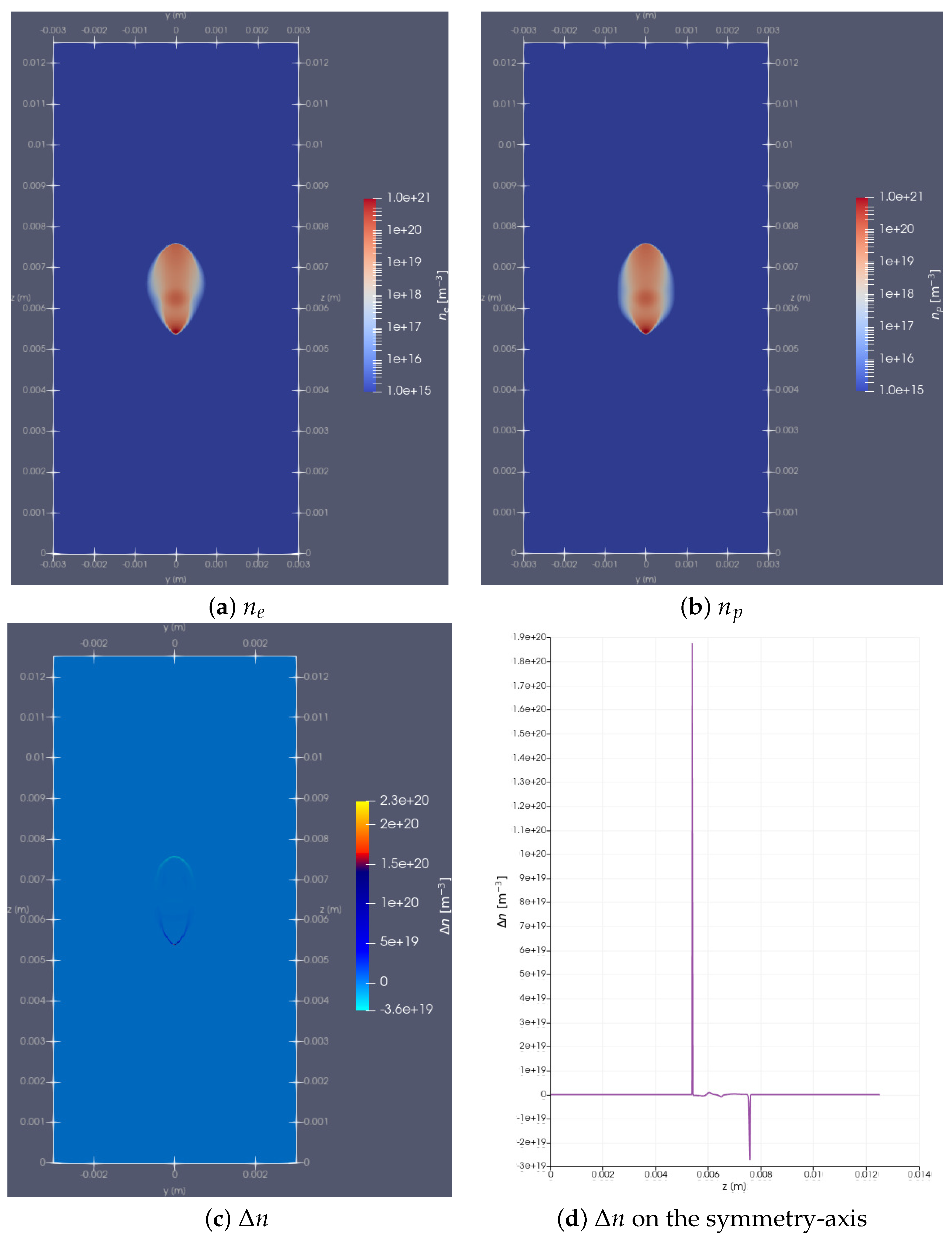
3.5. Streamer Modeling (Slides 17–22)

There are different ways of modeling electron avalanches and streamers. One approach is fluid modeling, where we apply the drift-diffusion equations for the densities of electrons ( n e ), positive ions ( n p ), and negative ions ( n n ) [61]
n e t + · D e n e μ e n e E = S p h + S i S a t t L e p
n p t = S p h + S i L e p L p n
n n t = S a t t L p n
together with the Poisson equation
Δ U = e 0 ϵ 0 n p n n n e .
Here, the temporal evolution of electrons and ions depends on the rates S i for electron impact ionization, S p h for photonization, S a t t for attachment, as well as electron-ion ( L e p ) and ion-ion ( L p n ) recombination. As we have discussed in Section 3.3, we need to take into account space charge effects created through electrons and ions by solving Equation (18) for the potential U which allows the calculation of the electric field through E = U . Charge separation results from the fact that we consider ions, which are much heavier than electrons, as immobile. Hence, for electrons, we also take into account their drift and their diffusion through
· D e n e μ e n e E
where μ e is the electron mobility, depending on the electric field, and D e is the electron diffusion.
The other approach to model streamers is particle modeling [62] where we actually trace individual electrons and integrate Newton’s equations
d p d t = e 0 E 0
d r d t = v
with the electron charge e 0 and the electric field E 0 , which is the superposition of the space charge field and the ambient field. Note that integrating (20) and (21) is not trivial, as the electric field generally depends on space and time, and we need to apply numerical schemes. There are two time steps: the time step t E to update the electric field, as well as the collision time step t c < t E , which is typically smaller than the electric field time step, hence there are some collisions within one field update. In between updating the electron momentum (20), we check for collisions where the probability is given by Equation (1). This allows the implementation of the physics for all collision types individually, i.e., elastic scattering, excitations, attachment, electron impact ionization and Bremsstrahlung for electrons. Hence, we can keep track of the individual positions, velocities, and energies of the particles. We solve Equations (20) and (21) and perform electron-gas collisions a couple of times until we have reached the electric field update time step and solve Equation (18) similar to the fluid code.
Both models have different advantages and disadvantages: The advantage of the fluid code is that it is relatively fast as we do not consider individual electrons; however, we lose physical accuracy because we do not describe individual electrons. The particle approach is normally more accurate but also much slower, although this really depends on a numerical experiment to be simulated.
Although every discharge starts with a single electron, typical streamer simulations start with an electron-ion Gaussian patch [22,35,37,63,64]
n e , i ( t = 0 , x , y , z ) = n e , 0 e r 2 + ( z z 0 ) 2 λ 2
where r = x 2 + y 2 , z 0 is the initial central height within the simulation domain, n e , 0 is the initial electron density, and λ the Gaussian decay length. Starting with (22) is a compromise between the computational burden to start with one single electron, developing into an electron avalanche and then streamer, and physical accuracy as the Gaussian (22) is designed such that it represents the size of the electron avalanche when the Raether-Meek criterion (13) is fulfilled, i.e., when the streamer regime starts [1,64]. The typical size λ of the patch is linked to the Raether-Meek criterion, the electron diffusion D, the electron mobility μ , the ambient electric field E a m b as well as to the ionization and attachment coefficients through [56,57,65]
λ = 4 D · 18 20 α i o n α a t t μ E a m b
which typically is on the order of 0.2 mm for air at ground pressure. As the total electron number is the volume integral of the electron density, the initial density can be approximated as
n e , 0 N e , 0 π 3 λ 3 10 18 10 20 m 3
for N e , 0 = 10 8 10 9 and typical values for λ at ground pressure [63].
Additionally, we need to specify the ambient field E a m b as well as the ambient gas mixture and the gas density. As an example, Figure 8 shows the electron density and the electric field after 1.38 ns for streamers in air (at ground pressure) in an ambient field of E a m b = 1.5 E k pointing downwards. Starting from a Gaussian patch, we observe the increase of the electron density and the electric field on both sides of the simulation domain. The growth on the upper tip is due to electrons moving upwards and performing electron impact ionization, while the growth at the lower tip is mediated by photonization (see Section 3.4). This growth is also what we typically observe in a discharge experiment where light is emitted from excited gas molecules excited by the electrons produced and accelerated in the streamer discharge. The electric field is reduced inside the channel and grows at the tips due to the production of electron-ion pairs and the subsequent charge separation. Inside the channel, there is an almost equal amount of negative and positive charge such that the field is shielded (see also Figure 7 for a discussion of space charge effects). Due to their larger mobility, electrons at the tips move away from the ions, leading to an increase in the electric field at the tips. The field at the positive tip is typically higher than at the negative tip. At the negative tip, electrons mainly move out of the tip, widening the charged region; in contrast, at the positive tip, electrons are dragged into the streamer tip such that the charge is concentrated on a smaller volume, leading to a higher field than at the negative tip. Subsequently, positive fronts accelerate more and, at some point, become faster than negative fronts. Usual velocities of streamers are on the order of 105–107 m/s. In such a streamer channel, the majority of electrons have energies of ≲10 eV; only a few have energies above 10 eV. Those are the electrons at the tip that ionize or excite the ambient gas. The maximum energy would typically be on the order of 100–200 eV, limited by the friction, see Figure 4.

3.6. Streamer Properties and Observations (Slides 23–24)

As aforementioned, streamer velocities are on the order of 105–107 m/s where positive streamers typically accelerate faster than negative streamers. Heating is negligible, as streamers are rather driven by the space charge effects (see Equation (18)), causing the electric field to grow at the tips. The high field at the tips accelerates the electrons, allowing them to excite air molecules. When deexciting, some of these states create photons in the visible wavelengths, becoming manifest as glowing streamer tips. At standard temperature and pressure (approx. 1 bar and 300 K), the streamer length is on the order of a few millimeters to centimeters with a width of a few millimeters.
In the previous sections, we have mainly discussed streamer avalanches and streamer properties in air, but they also appear in other gas mixtures. For example, there have been laboratory experiments of streamer discharges in a Venus-like atmosphere CO2:N2 = 96.5%:3.5%, and in the Jovian atmosphere H2:He = 89.8%:10.2% [36], while there have also been observations of streamer discharges on Venus [66]. In previous work, we have simulated streamers in the atmosphere of Saturn’s moon Titan (N2:CH4 = 98.4%:1.6%) [35] as well as in the atmospheres suggested for Primordial Earth (N2:CO2:H2O:H2:CO = 80%:18.89%:1%:0.1%:0.01% or H2O:CH4:NH3:H2 = 37.5%: 25%:25%:12.5%) [37]. Apart from their relevance as precursors of lightning, streamers in various gas mixtures also have technological applications, such as N2:O2 with the addition of methane used for combustion [38], or streamers in SF6 for switching applications [52].

3.7. Streamers as Precursors to Lightning Leaders and Their Relation to Plasma Chemistry (Slides 25–26)

After streamer inception, additional processes occur on longer timescales. In particular, the energy transfer from charged to neutral species, i.e., from the electrons and ions to the gas molecules, as well as the energy transfer from so-called vibrational to translational states, increase the energy in the system heating the discharge channel transiting the cold streamer to the hot lightning leader [4]. The details of this process are out of the scope of this paper and might be subject to a follow-up video. Just note that the existence of streamers is necessary to form the km-long lightning channels.
As mentioned in Section 3.1, transient luminous events appear above thunderstorms [6]. Among them, there are sprite streamers, with their large electric fields and their local heating, triggering the plasma chemistry of the environment [67]. This involves reactions of nitrogen, oxygen, carbon, and other species in our atmosphere, forming further species such as methane CH 4 , ozone O 3 , nitrogen oxides NO x , or nitrous oxides N2O [67].

4. Conclusions and Outlook

We have presented an audiovisual introduction to streamer physics, which can be used as an easy introduction for students and early researchers in the field of atmospheric electricity. The red thread ranges from the motion of single electrons over the formation of electron avalanches to the formation of streamers, at the end touching upon plasma chemistry and the formation of lightning leaders. We have provided details about cross-sections and scattering probabilities, as well as an extended discussion of the friction force in air. We also describe how to model streamers, explain the different propagation mechanisms for negative and positive streamer tips, and provide an overview of streamer properties. Finally, we briefly discuss plasma chemistry and give an outlook on how streamers turn into long, bright, lightning leader channels. Of course, there is plenty of more written material that can serve as an introduction to streamer physics with more depth that can be provided in the Supplementary Video, among which there are excellent review papers [40,42,68,69] and books on lightning physics [1,41,70,71] together with the references mentioned along this review. This introduction might additionally give a hint of how to present discharge physics to a broader audience. Finally, streamers are just one part of the research field of atmospheric electricity. This introduction could serve as a stepping stone for a series of videos reviewing the physics of leaders, transient luminous events, terrestrial gamma-ray flashes, etc.

Supplementary Materials

The following supporting information can be downloaded at: https://www.mdpi.com/article/10.3390/atmos16070757/s1, Video S1: An audiovisual introduction to streamer physics. This video provides a first overview of the physics of the collision-dominated motion of electrons as well as of streamers.

Funding

C.K. has received funding from the Independent Research Fund Denmark (grant 1054-00104). This research was funded by Independent Research Fund Denmark grant number 1054-00104.

Institutional Review Board Statement

Not applicable.

Informed Consent Statement

Not applicable.

Data Availability Statement

No new data were created or analyzed in this study.

Acknowledgments

We thank Angel Ricardo Jara Jimenez and Morten Jung Westermann for providing numerical support to make the Figure 7 and Figure 8 as well as the figures and videos on slides 19–21. We thank Ramona Uthmann for video editing.

Conflicts of Interest

The authors declare no conflict of interest.

Appendix A. Acknowledgment for Figures Used in the Presentation

For the following figures from the presentation, we summarize their origin and acknowledge the copyright owner permitting us to reuse the figure, or give licence details.
Table A1. Overview of provided figures in the presentation including reference and copyright.
SlideFigureReferenceCopyright/License
3top left: lightning flash[50]CC BY-SA 4.0
top right: discharge inception from needle electrode[51]Permission granted by J. Mizeraczyk et al. [51]
bottom left: overview of Transient Luminous Events[6]Copyright ©2003, The American Association for the Advancement of Science
bottom right: sketch of plasma medice deviceOpen Day 2013, Centrum Wiskunde & Informatica (CWI), Amsterdam, NL
9Visualisation of electron discharge[55]CC BY-SA 3.0
14negative streamer propagation[1]Copyright by Springer Verlag Berlin Heidelberg New York
15positive streamer propagation[1]Copyright by Springer Verlag Berlin Heidelberg New York
25right: lightning flash[50]CC BY-SA 4.0
26top: overview of Transient Luminous Events[6]Copyright ©2003, The American Association for the Advancement of Science
bottom: excerpt of a table of chemical reactions[67]Copyright 2008 by the American Geophysical Union

References

  1. Raizer, Y. Gas Discharge Physics; Springer: Berlin/Heidelberg, Germany, 1991. [Google Scholar]
  2. Raizer, Y.; Milikh, G.; Shneider, M.; Novakovski, S. Long streamers in the upper atmosphere above thundercloud. J. Phys. D Appl. Phys. 1998, 31, 3255–3264. [Google Scholar] [CrossRef]
  3. Moss, G.; Pasko, V.; Liu, N.; Veronis, G. Monte Carlo model for analysis of thermal runaway electrons in streamer tips in transient luminous events and streamer zones of lightning leaders. J. Geophys. Res. 2006, 111, A02307. [Google Scholar] [CrossRef]
  4. da Silva, C.; Pasko, V. Dynamics of streamer-to-leader transition at reduced air densities and its implications for propagation of lightning leaders and gigantic jets. J. Geophys. Res. 2013, 118, 13561–13590. [Google Scholar] [CrossRef]
  5. Montanyà, J.; van der Velde, O.; Williams, E. The start of lightning: Evidence of bidirectional lightning initiation. Nat. Sci. Rep. 2015, 5, 15180. [Google Scholar] [CrossRef]
  6. Neubert, T. On Sprites and Their Exotic Kin. Science 2003, 300, 747–749. [Google Scholar] [CrossRef]
  7. Cummer, S.; Jaugey, N.; Li, J.; Lyons, W.; Nelson, T.; Gerken, E. Submillisecond imaging of sprite development and structure. Geophys. Res. Lett. 2006, 33, L04104. [Google Scholar] [CrossRef]
  8. Pasko, V. Red sprite discharges in the atmosphere at high altitude: The molecular physics and the similarity with laboratory discharges. Plasma Sour. Sci. Technol. 2007, 16, S13–S29. [Google Scholar] [CrossRef]
  9. Qin, J.; Celestin, S.; Pasko, V. Formation of single and double-headed streamers in sprite-halo events. Geophys. Res. Lett. 2012, 39, L05810. [Google Scholar] [CrossRef]
  10. Starikovskaia, S. Plasma-assisted ignition and combustion: Nanosecond discharges and development of kinetic mechanisms. J. Phys. D Appl. Phys. 2014, 47, 353001. [Google Scholar] [CrossRef]
  11. Popov, N. Kinetics of plasma-assisted combustion:effect of non-equilibrium excitation on the ignition and oxidation of combustible mixtures. Plasma Sour. Sci. Technol. 2016, 25, 043002. [Google Scholar] [CrossRef]
  12. Fridman, G.; Friedman, G.; Gutsol, A.; Shekhter, A.; Vasilets, V.; Fridman, A. Applied plasma medicine. Plasma Process. Polym. 2008, 5, 503–533. [Google Scholar] [CrossRef]
  13. Laroussi, M. From killing bacteria to destroying cancercells: 20 years of plasma medicine. Plasma Process. Polym. 2014, 11, 1138–1141. [Google Scholar] [CrossRef]
  14. Starikovskiy, A.; Aleksandrov, N. Blocking streamer development by plane gaseous layers of various densities. Plasma Sour. Sci. Technol. 2020, 29, 034002. [Google Scholar] [CrossRef]
  15. Starikovskiy, A.; Aleksandrov, N. How pulse polarity and photoionization control streamer discharge development in long air gaps. Plasma Sour. Sci. Technol. 2020, 29, 075004. [Google Scholar] [CrossRef]
  16. Boggs, S.; Schramm, H.H. Current interruption and switching in sulphur hexafuoride. IEEE Electr. Insul. Mag. 1990, 6, 12–17. [Google Scholar] [CrossRef]
  17. Christophorou, L.; Olthoff, J.; Van Brunt, R. Sulfur hexafuoride and the electric power industry. IEEE Electr. Insul. Mag. 1997, 13, 20–24. [Google Scholar] [CrossRef]
  18. Zhang, B.; Uzelac, N.; Cao, Y. Fluoronitrile/CO2 mixture as an eco-friendly alternative to SF6 for medium voltage switchgears. IEEE Trans. Dielectr. Electr. Insul. 2018, 25, 1340–1350. [Google Scholar] [CrossRef]
  19. Zheleznyak, M.; Mnatsakanyan, A.; Sizykh, S. Photoionization of nitrogen and oxygen mixtures by radiation from a gas discharge. High Temp. 1982, 20, 357–362. [Google Scholar]
  20. Pancheshnyi, S. Role of electronegative gas admixtures in streamer start, propagation and branching phenomena. Plasma Sour. Sci. Technol. 2005, 14, 645–653. [Google Scholar] [CrossRef]
  21. Luque, A.; Ebert, U.; Montijn, C.; Hundsdorfer, W. Photoionisation in negative streamers: Fast computations and two propagation modes. Appl. Phys. Lett. 2007, 90, 081501. [Google Scholar] [CrossRef]
  22. Köhn, C.; Chanrion, O.; Neubert, T. The influence of bremsstrahlung on electric discharge streamers in N2, O2 gas mixtures. Plasma Sour. Sci. Technol. 2017, 26, 015006. [Google Scholar] [CrossRef]
  23. Nguyen, C.; van Deursen, A.; Ebert, U. Multiple x-ray bursts from long discharges in air. J. Phys. D. Appl. Phys. 2008, 41, 234012. [Google Scholar] [CrossRef]
  24. Rahman, M.; Cooray, V.; Ahmad, N.; Nyberg, J.; Rakov, V.; Sharma, S. X rays from 80-cm long sparks in air. Geophys. Res. Lett. 2008, 35, L06805. [Google Scholar] [CrossRef]
  25. Nguyen, C.; van Deursen, A.; van Heesch, E.; Winands, G.; Pemen, A. X-ray emission in streamer-corona plasma. J. Phys. D Appl. Phys. 2010, 43, 025202. [Google Scholar] [CrossRef]
  26. Kochkin, P.; Nguyen, C.; van Deursen, A.; Ebert, U. Experimental study of hard x-rays emitted from metre-scale positive discharges in air. J. Phys. D Appl. Phys. 2012, 45, 425202. [Google Scholar] [CrossRef]
  27. Kochkin, P.; van Deursen, A.; Ebert, U. Experimental study on hard x-rays emitted from metre-scale negative discharges in air. J. Phys. D Appl. Phys. 2014, 48, 025202. [Google Scholar] [CrossRef]
  28. Kochkin, P.; Köhn, C.; Ebert, U.; van Deursen, A. Analyzing x-ray emissions from meter-scale negative discharges in ambient air. Plasma Sour. Sci. Technol. 2016, 25, 044002. [Google Scholar] [CrossRef]
  29. Fishman, G.J.; Bhat, P.N.; Mallozzi, R.; Horack, J.M.; Koshut, T.; Kouveliotou, C.; Pendleton, G.N.; Meegan, C.A.; Wilson, R.B.; Paciesas, W.S.; et al. Discovery of intense gamma-ray flashes of atmospheric origin. Science 1994, 264, 1313–1316. [Google Scholar] [CrossRef]
  30. Briggs, M.; Fishman, G.; Connaughton, V.; Bhat, P.; Paciesas, W.; Preece, R.; Wilson-Hodge, C.; Chaplin, V.L.; Kippen, R.M.; von Kienlin, A.; et al. First results on terrestrial gamma ray flashes from the Fermi gamma-ray burst monitor. J. Geophys. Res. 2010, 115, A07323. [Google Scholar] [CrossRef]
  31. Briggs, M.S.; Xiong, S.; Connaughton, V.; Tierney, D.; Fitzpatrick, G.; Foley, S.; Grove, J.E.; Chekhtman, A.; Gibby, M.; Fishman, G.J.; et al. Terrestrial gamma-ray flashes in the Fermi era: Improved observations and analysis methods. J. Geophys. Res. 2013, 118, 3805–3830. [Google Scholar] [CrossRef]
  32. Østgaard, N.; Neubert, T.; Reglero, V.; Ullaland, K.; Yang, S.; Genov, G.; Marisaldi, M.; Mezentsev, A.; Kochkin, P.; Lehtinen, N.; et al. First 10 Months of TGF Observations by ASIM. J. Geophys. Res. Atmos. 2019, 124, 14024–14036. [Google Scholar] [CrossRef]
  33. Köhn, C.; Heumesser, M.; Chanrion, O.; Nishikawa, K.; Reglero, V.; Neubert, T. The Emission of Terrestrial Gamma Ray Flashes From Encountering Streamer Coronae Associated to the Breakdown of Lightning Leaders. Geophys. Res. Lett. 2020, 47, e2020GL089749. [Google Scholar] [CrossRef]
  34. Heumesser, M.; Chanrion, O.; Neubert, T.; Christian, H.J.; Dimitriadou, K.; Gordillo-Vazquez, F.J.; Luque, A.; Pérez-Invernón, F.J.; Blakeslee, R.J.; Østgaard, N.; et al. Spectral Observations of Optical Emissions Associated with Terrestrial Gamma-Ray Flashes. Geophys. Res. Lett. 2021, 48, e2020GL090700. [Google Scholar] [CrossRef] [PubMed]
  35. Köhn, C.; Dujko, S.; Chanrion, O.; Neubert, T. Streamer propagation in the atmosphere of Titan and other N2:CH4 mixtures compared to N2:O2 mixtures. Icarus 2019, 333, 294–305. [Google Scholar] [CrossRef]
  36. Dubrovin, D.; Nijdam, S.; van Veldhuizen, E.; Ebert, U.; Yair, Y.; Price, C. Sprite discharges on Venus and Jupiter-like planets: A laboratory investigation. J. Geophys. Res. 2010, 115, A00E34. [Google Scholar] [CrossRef]
  37. Köhn, C.; Chanrion, O.; Enghoff, M.; Dujko, S. Streamer discharges in the atmosphere of Primordial Earth. Geophys. Res. Lett. 2022, 49, e2021GL09750. [Google Scholar] [CrossRef]
  38. Bouwman, D.; Teunissen, J.; Ebert, U. 3D particle simulations of positiveair–methane streamers for combustion. Plasma Sour. Sci. Technol. 2022, 31, 045023. [Google Scholar] [CrossRef]
  39. Ebert, U.; Sentman, D. Streamers, sprites, leaders, lightning: From micro- to macroscales. J. Phys. D Appl. Phys. 2008, 41, 230301. [Google Scholar] [CrossRef]
  40. Ebert, U.; Nijdam, S.; Li, C.; Luque, A.; Briels, T.; van Veldhuizen, E. Review of recent results on streamer discharges and discussion of their relevance for sprites and lightning. J. Geophys. Res. Space Phys. 2010, 115, A00E43. [Google Scholar] [CrossRef]
  41. Cooray, V. An Introduction to Lightning; Springer: Berlin/Heidelberg, Germany, 2015. [Google Scholar]
  42. Nijdam, S.; Teunissen, J.; Ebert, U. The physics of streamer discharge phenomena. Plasma Sour. Sci. Technol. 2020, 29, 103001. [Google Scholar] [CrossRef]
  43. Hartley, J.; Davies, I. Note-taking: A critical review. Program. Learn. Educ. Technol. 1978, 15, 207–224. [Google Scholar] [CrossRef]
  44. Wankat, P. The Effective, Efficient Professor: Teaching Scholarship and Service; Pearson: London, UK, 2001. [Google Scholar]
  45. Carstens, D.; Doss, S.; Kies, S. Social Media Impact on Attention Span. J. Manag. Eng. Integr. 2018, 11, 20–27. [Google Scholar]
  46. Ray, E. Outreach, engagement will keep academia relevant to twenty-first century societies. J. Pub. Serv. Outreach 1999, 4, 21–27. [Google Scholar]
  47. Ecklund, E.; James, S.; Lincoln, A. How Academic Biologists and Physicists View ScienceOutreach. PLoS ONE 2012, 7, e36240. [Google Scholar] [CrossRef] [PubMed]
  48. Köhn, C. Blitze auf der Urerde; Science Slam Hamburg: Hamburg, Germany, 2022; Available online: https://www.youtube.com/watch?v=gYcprqUemMQ (accessed on 10 June 2025). (In German)
  49. St Andrews Centre for Exoplanet Science. Available online: https://exoplanets.wp.st-andrews.ac.uk/ (accessed on 10 June 2025).
  50. Vidinovski, F. Wikipedia: A Lightning Strike as Seen from the Village of Dolno Sonje, in a Rural Area South of Skopje, North Macedonia. 2020. Available online: https://en.wikipedia.org/wiki/Lightning_strike#/media/File:Rural_nightime_lightning_strike.png (accessed on 10 June 2025).
  51. Mizeraczyk, J.; Kanazawa, S.; Ohkubo, T. Progress in the Visualization of Filamentary Gas Discharges. Part 2: Visualization of DC Positive Corona Discharges. J. Adv. Oxid. Technol. 2004, 7, 20–30. [Google Scholar] [CrossRef]
  52. Boakye-Mensah, F.; Bonifaci, N.; Hanna, R.; Niyonzima, I.; Timoshkin, I. Modelling of Positive Streamers in SF6 Gas under Non-Uniform Electric Field Conditions: Effect of Electronegativity on Streamer Discharges. Multi. Sci. J. 2022, 5, 255–276. [Google Scholar] [CrossRef]
  53. Plasma Data Exchange Project: LXCat. Available online: https://nl.lxcat.net/home/ (accessed on 10 June 2025).
  54. Gurevich, A. On the theory of runaway electrons. Sov. Phys. JETP-USSR 1961, 12, 904–912. [Google Scholar]
  55. Dougsim. Wikipedia: Visualisation of a Townsend Avalanche. 2012. Available online: https://en.wikipedia.org/wiki/Townsend_discharge#/media/File:Electron_avalanche.gif (accessed on 10 June 2025).
  56. Raether, H. Die Entwicklung der Elektronen in den Funkenkanal. Zeit. F. Phys. 1939, 112, 464–489. [Google Scholar] [CrossRef]
  57. Meek, J. A theory of spark discharge. Phys. Rev. 1940, 57, 722–728. [Google Scholar] [CrossRef]
  58. Montijn, C.; Ebert, U. Diffusion correction to the Raether-Meek criterion for the avalanche-to-streamer transition. J. Phys. D Appl. Phys. 2006, 39, 2979–2992. [Google Scholar] [CrossRef]
  59. Peeters, S.; Mirpour, S.; Köhn, C.; Nijdam, S. A Model for Positive Corona Inception From Charged Ellipsoidal Thundercloud Hydrometeors. J. Geophys. Res. Atmos. 2022, 127, e2021JD035505. [Google Scholar] [CrossRef]
  60. Li, C.; Teunissen, J.; Nool, M.; Hundsdorfer, W.; Ebert, U. A comparison of 3D fluid, particle and hybrid model for negative streamers. Plasma Sources Sci. Technol. 2012, 21, 055019. [Google Scholar] [CrossRef]
  61. Kulikovsky, A. Positive streamer between parallel plate electrodes in atmospheric pressure air. J. Phys. D Appl. Phys. 1997, 30, 441–450. [Google Scholar] [CrossRef]
  62. Chanrion, O.; Neubert, T. A PIC-MCC code for simulation of streamer propagation in air. J. Comp. Phys. 2008, 227, 7222–7245. [Google Scholar] [CrossRef]
  63. Liu, N.; Pasko, V. Effects of photoionization on propagation and branching of positive and negative streamers in sprites. J. Geophys. Res. 2004, 109, A04301. [Google Scholar]
  64. Wormeester, G.; Pancheschnyi, S.; Luque, A.; Nijdam, S.; Ebert, U. Probing photo-ionization: Simulations of positive streamers in varying N2:O2-mixtures. J. Phys. D Appl. Phys. 2010, 43, 505201. [Google Scholar] [CrossRef]
  65. Köhn, C.; Chanrion, O.; Neubert, T. The Sensitivity of Sprite Streamer Inception on the Initial Electron-Ion Patch. J. Geophys. Res. Space Phys. 2019, 124, 3083–3099. [Google Scholar] [CrossRef]
  66. Pérez-Invernón, F.; Luque, A.; Gordillo-Vázquez, F. Mesospheric optical signatures of possible lightning on Venus. J. Geophys. Res. Space Phys. 2016, 121, 7026–7048. [Google Scholar] [CrossRef]
  67. Sentman, D.; Stenbaek-Nielsen, H.; McHarg, M.; Morrill, J. Plasma chemistry of sprite streamers. J. Geophys. Res. 2008, 113, D11112. [Google Scholar] [CrossRef]
  68. Ebert, U.; Montijn, C.; Briels, T.; Hundsdorfer, W.; Meulenbroek, B.; Rocco, A.; van Veldhuizen, E. The multiscale nature of streamers. Plasma Sour. Sci. Technol. 2006, 15, S118–S129. [Google Scholar] [CrossRef]
  69. Dwyer, J.R.; Uman, M.A. The physics of lightning. Phys. Rep. 2014, 534, 147–241. [Google Scholar] [CrossRef]
  70. Uman, M. The Lightning Discharge; Academic Press: London, UK, 1987. [Google Scholar]
  71. Rakov, V.; Uman, M. Lightning: Physics and Effects; Cambridge University Press: Cambridge, UK, 2003. [Google Scholar]
Figure 1. General setup of the electron motion in an ambient gas: While electrons accelerate in the ambient electric field E a m b , they collide with the gas molecules. They scatter elastically as well as excite (orange) or ionize (blue) the gas molecules.
Atmosphere 16 00757 g001
Figure 2. Geometric interpretation of electrons (small black circles) with velocity v colliding at air molecules (red circles) within a time step Δ t . The yellow area symbolizes the cross-section as a geometric interaction area (3).
Atmosphere 16 00757 g002
Figure 3. (a) The elastic scattering cross-section of electrons at N 2 and O 2 and (b) the total cross-section for an excitation channel of N 2 and O 2 as a function of electron energy [53]. The blue line depicts the geometric cross-section of 7 × 10 20 m 2 (which is approximately the same for N 2 and O 2 ).
Atmosphere 16 00757 g003
Figure 4. The friction force of electrons in the air as a function of the electron energy [3,54]. The dotted lines show the characteristic fields for runaway breakdown ( E t h ), classical breakdown ( E k ), and thermal runaway ( E c ). The green arrows indicate the equilibrium point of the friction force and the breakdown field E k . The red arrow indicates the runaway regime.
Atmosphere 16 00757 g004
Figure 5. Visualization of an electron avalanche [55]. In the electric field between the cathode and anode, electrons move and ionize air molecules, yielding an electron avalanche.
Atmosphere 16 00757 g005
Figure 6. The ionization ( α i o n ) and attachment ( α a t t ) flux coefficients of electrons in air as a function of the reduced electric field E / n a m b . The black circle indicates the equilibrium point (14) defining the breakdown field E k . The data are reproduced from [60].
Atmosphere 16 00757 g006
Figure 7. A sketch of the electron (a) and positive ion density (b) of a streamer discharge in air at x = 0 in an ambient field of 50 kV cm 1 after 1.11 ns; the negative tip propagates upwards while the positive tip propagates downwards. (c) The space charge density Δ n = n p n n n e is the density difference of positive and negative charges; (d) the space charge density as a function of z for x = y = 0 .
Atmosphere 16 00757 g007
Figure 8. The electron density (contour plot (a) and along the z-axis (c)) and the electric field (b,d) of a streamer discharge in air after in an ambient field of 1.5 E k = 48 kV/cm after 1.38 ns.
Atmosphere 16 00757 g008
Disclaimer/Publisher’s Note: The statements, opinions and data contained in all publications are solely those of the individual author(s) and contributor(s) and not of MDPI and/or the editor(s). MDPI and/or the editor(s) disclaim responsibility for any injury to people or property resulting from any ideas, methods, instructions or products referred to in the content.

