Assessing the Reliability of Seasonal Data in Representing Synoptic Weather Types: A Mediterranean Case Study

Abstract

Seasonal climate forecasts are an essential tool for providing early insight into weather-related impacts and supporting decision-making in sectors such as agriculture, energy, and disaster management. Accurate representation of atmospheric circulation at the seasonal scale is essential, especially in regions such as the Eastern Mediterranean, where complex synoptic patterns drive significant climate variability. The aim of this study is to perform a comparison of weather type classifications between ERA5 reanalysis and seasonal forecasts in order to assess the ability of seasonal data to capture the synoptic patterns over the Eastern Mediterranean. For this purpose, we introduce a regional seasonal forecasting framework based on the state-of-the-art Advanced Research WRF (WRF-ARW) model. A series of sensitivity experiments were also conducted to evaluate the robustness of the model’s performance under different configurations. Moreover, the ability of seasonal data to reproduce observed trends in weather types over the historical period is also examined. The classification results from both ERA5 and seasonal forecasts reveal a consistent dominance of anticyclonic weather types throughout most of the year, with a particularly strong signal during the summer months. Model evaluation indicates that seasonal forecasts achieve an accuracy of approximately 80% in predicting the daily synoptic condition (cyclonic or anticyclonic) up to three months in advance. These findings highlight the promising skill of seasonal datasets in capturing large-scale circulation features and their associated trends in the region.

1. Introduction

The accelerating pace of climate change presents a growing set of challenges for modern societies. From extreme weather events and devastating wildfires to crop failures and rising climate-related health concerns, the impacts of a shifting climate are becoming increasingly evident [1,2]. This is particularly critical in vulnerable regions such as the Mediterranean, where climate extremes are intensifying at an alarming rate. The Mediterranean has been identified as a climate change hotspot, experiencing higher-than-average temperature increases, prolonged droughts, and a rising frequency of extreme weather events [3,4,5]. These changes not only threaten local ecosystems but also pose significant risks to agriculture, water resources, and human health [6]. As a result, the demand for more accurate and timely climate predictions has never been greater, particularly for regions like the Mediterranean that are at the frontline of climate change impacts.

Understanding and predicting seasonal climate variations is crucial for decision-making. Seasonal climate forecasts provide valuable probabilistic assessments of climate conditions over periods of months, enabling policymakers and stakeholders to implement proactive measures to mitigate the socioeconomic impacts of climate variability [7,8,9]. Unlike short-term weather forecasts, which predict atmospheric conditions on a daily basis, seasonal forecasts rely on large-scale climate drivers such as ocean–atmosphere interactions, stratospheric variability, and land surface conditions to project temperature and precipitation trends.

In recent years, advancements in weather prediction models have led to significant improvements in forecasting accuracy. Short-term weather forecast predictability, spanning up to 7 to 10 days, presents a continuous rising trend, although studies suggest the existence of a predictability limit [10,11]. These improvements have been driven by better numerical modeling techniques, increased computational power, and the integration of high-resolution satellite observations into forecasting systems. Meanwhile, long-term climate projections—those extending decades into the future—are generally considered robust in capturing large-scale trends and the influence of anthropogenic forcing [12]. However, a major challenge persists in bridging the gap between these two timescales, where forecasting remains more uncertain. This is where seasonal forecasting comes into play. By leveraging statistical and dynamical models, seasonal forecast systems aim to predict climate conditions weeks to months in advance [13]. These models rely on global-scale interactions between the atmosphere, oceans, land, and ice systems to generate probabilistic outlooks. While not as precise as short-term weather forecasts, seasonal forecasts provide invaluable insights into temperature anomalies, precipitation patterns, and other climate indicators, helping governments, industries, and communities better prepare for potential climate-related risks [14]. The concept of seasonal forecasting emerged in the mid-20th century, initially relying on statistical relationships between atmospheric circulation patterns and oceanic conditions [15]. The research development of El Niño–Southern Oscillation (ENSO) in the 1980s provided a breakthrough, establishing a connection between oceanic variability and seasonal climate patterns, as it is considered the major source of predictability [16,17]. ENSO significantly influences global seasonal climate variability through its impact on atmospheric circulation patterns, thereby affecting temperature and precipitation anomalies across various regions [18]. Since then, advances in global climate modeling and data assimilation techniques have significantly improved the skill and reliability of seasonal forecasts [19].

Seasonal forecasts are primarily generated through dynamical and statistical methods. Dynamical models, such as those used by the European Center for Medium-Range Weather Forecasts (ECMWF) and the National Centers for Environmental Prediction (NCEP), rely on coupled ocean–atmosphere general circulation models (GCMs) to simulate future climate states [13,17]. These models incorporate observations from satellite and ground-based systems to provide probabilistic climate outlooks. Statistical methods, on the other hand, use historical data and empirical relationships to make predictions, often complementing dynamical models in hybrid forecasting systems [17].

The advantages of seasonal forecasts are substantial. They provide early warnings of extreme climate events, such as droughts, heatwaves, and hurricanes, allowing decision-makers to implement proactive mitigation measures [8]. In agriculture, seasonal forecasts assist farmers in optimizing crop selection and irrigation planning, reducing the economic impact of unfavorable weather conditions [20]. Similarly, the energy sector benefits from improved predictions of temperature-driven electricity demand, facilitating efficient resource allocation [21,22].

Despite these benefits, seasonal forecasting faces several limitations. One major challenge is the inherent uncertainty associated with long-range predictions due to the chaotic nature of the atmosphere. Model biases, inaccuracies in initial conditions, and limited predictability of some climate drivers contribute to errors in seasonal forecasts [23]. Furthermore, regional forecasting skills vary, and certain areas exhibit lower predictability due to weak ocean–atmosphere coupling or complex land surface interactions [24]. Efforts to improve seasonal forecasting accuracy continue, with advancements in data assimilation, ensemble prediction techniques, and machine learning-based approaches offering promising developments [25,26].

Another fundamental aspect of meteorology and climatology is understanding and classifying atmospheric circulation patterns. Weather type classification (WTC) methods, often referred to as Weather Pattern Classification or Circulation Type Classification, provide a structured framework for analyzing and interpreting atmospheric dynamics. These classifications serve as essential tools in various applications, including climate variability studies, extreme weather event analysis, forecasting, and environmental impact assessments [27]. The importance of weather classification arises from the complex and inherently chaotic nature of the atmosphere. Atmospheric circulation governs large-scale weather phenomena, and by categorizing recurrent circulation types, scientists can better comprehend long-term climate trends and short-term weather variability. Moreover, such classifications enhance the predictability of specific weather conditions, aiding sectors such as agriculture, hydrology, and energy management.

In general, weather classification methods can be categorized into subjective and objective approaches. Subjective classifications rely on expert judgment and manual analysis of synoptic charts, a method historically used in meteorological studies. Notable examples include the Grosswetterlagen classification in Europe [28] and the Lamb Weather Types for the British Isles [29]. While these approaches provide valuable insights, they are often limited by their reliance on expert interpretation and potential inconsistencies across different analysts. Objective classification methods, on the other hand, employ statistical and computational techniques to categorize circulation types based on large datasets of meteorological variables. These methods include clustering algorithms, principal component analysis, and machine learning techniques [30,31]. They have the advantage of being more consistent, efficient, and less time-consuming. Also, they have the advantage of reduced subjectivity, minimizing personal biases [31,32]. On the other hand, they can have limitations such as limited flexibility and computational complexity. They can also have difficulties in describing regional characteristics and, of course, there is still a degree of subjectivity, especially in the methods and thresholds used [33]. There is a large number of different WTCs that have been applied worldwide using different approaches. The COST Action 733 initiative, focused on standardizing and applying weather type classifications across European regions, compiled a range of WTCs and created a platform to evaluate 17 objective and five subjective classification methods for the European/North Atlantic area [31].

Different classifications have been applied in the Mediterranean region. Ref. [34] created an empirical classification based on cluster analysis. Ref. [35] developed an automated classification for Greece using MSLP and 500 hPa gridded data, identifying twenty different weather types. Ref. [36] created a classification method for the Mediterranean that can be used throughout Europe using 500 hPa geopotential height anomalies.

Weather types (WTs) are a coding of the synoptic conditions in a region and can be used as a tool for both statistical analysis and also in the evaluation of seasonal forecasts. The aim of this paper is to compare weather type classifications using reanalysis data and seasonal forecasts produced by the state-of-the-art Advanced Research WRF (WRF-ARW) model for the period 1981–2016. This is performed in order to find out whether the seasonal forecasts are able to identify synoptic conditions months in advance, and help in providing early warnings for sectors such as agriculture, water management, tourism, etc.

In this context, the present study aims to evaluate the ability of seasonal forecasts to capture the prevailing synoptic patterns over the Eastern Mediterranean by comparing WT classifications derived from ERA5 reanalysis data [37] and seasonal forecast outputs. Through this comparison, we seek to assess the skill of seasonal forecasting systems in reproducing large-scale atmospheric circulation types, thereby supporting their potential use in early-warning applications for climate-sensitive sectors.

2. Data and Methodology

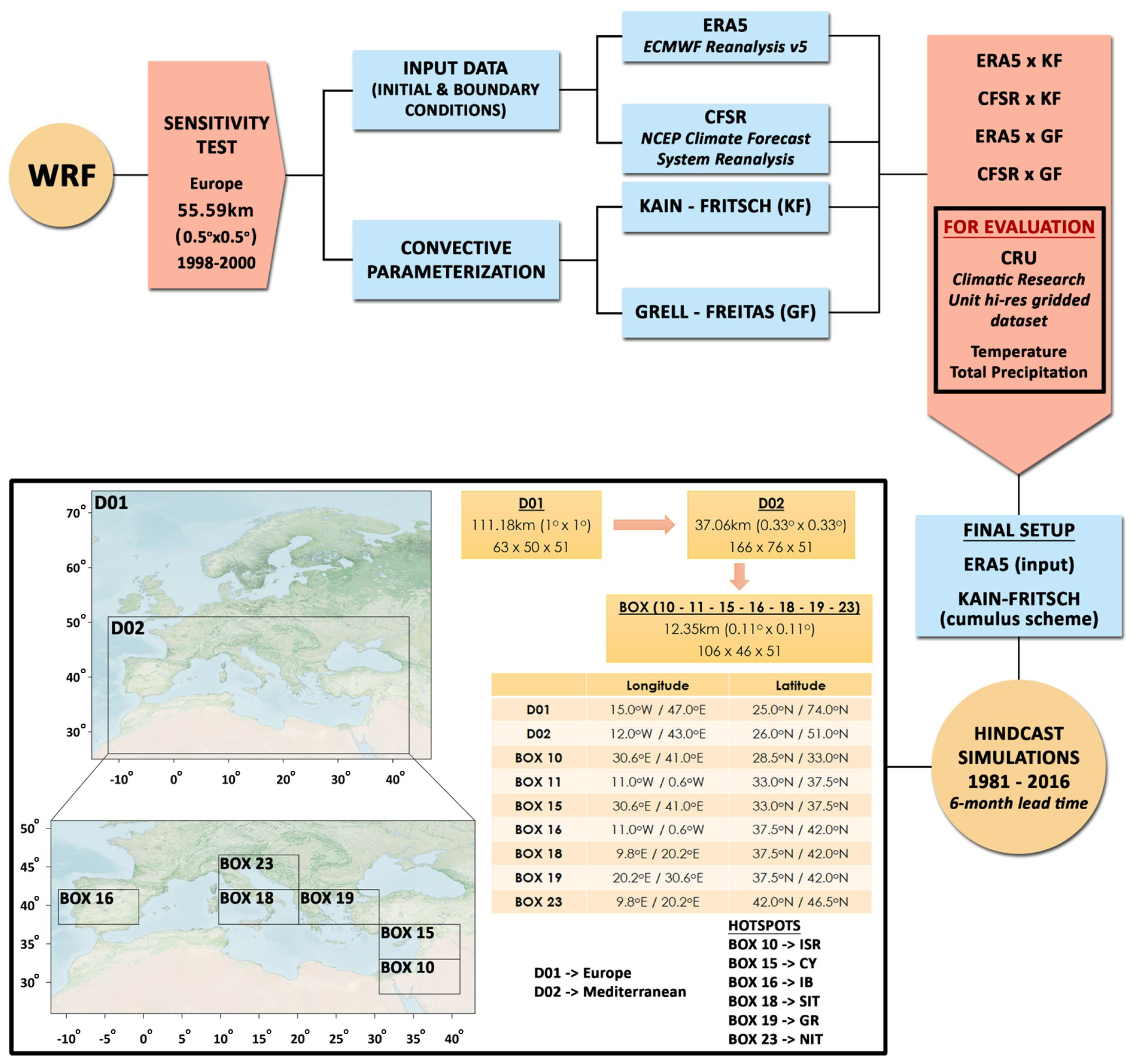
2.1. WRF-ARW Seasonal Forecast Model

This study utilizes version 4.5 of the Weather Research and Forecasting (WRF) Model, a state-of-the-art mesoscale numerical weather prediction system designed for both research and operational forecasting applications [38]. WRF is widely used across a range of meteorological scales, from regional to global. The WRF modeling system includes two primary dynamic cores: the Non-Hydrostatic Mesoscale Model (NMM), commonly used in forecasting, and the Advanced Research WRF (ARW) core, intended for research applications. For this study, the WRF-ARW core was selected due to its flexibility in configuring physical and dynamical processes, which makes it more suitable for downscaling experiments. The model was configured using a two-domain nested setup, with the outer domain at 12 km × 12 km resolution and the inner domain at 4 km × 4 km, including 31 vertical levels. The methodology described below is illustrated in Figure 1. All the simulations mentioned below are performed in the Aristotle University of Thessaloniki (AUTh) High-Performance Computing (HPC) Infrastructure and Resources.

2.1.1. Sensitivity Test

A series of sensitivity simulations were conducted to determine the most appropriate input dataset—for the initial and boundary conditions—and cumulus convection scheme. The sensitivity experiments covered a domain extending across Europe, with a coarse horizontal resolution of 55.59 km × 55.59 km ($0.5^{\circ }\times 0.5^{\circ }$). Four simulations were performed during the period of 1998–2000, which is a typical time span for such tests, with an additional spin-up year to allow the model to reach a stable state. Two different reanalysis datasets were used to provide initial and boundary conditions: (a) the ECMWF fifth-generation atmospheric reanalysis data (ERA5) and (b) the NCEP Climate Forecast System Reanalysis (CFSR). Both datasets are commonly employed in WRF studies and were processed accordingly to ensure compatibility with the model input requirements. To assess the model’s sensitivity to cumulus convection parameterization, two schemes were tested: the Grell–Freitas (GF) and the Kain–Fritsch (KF) schemes.

Model output was evaluated for 2 m temperature, as well as 2 m minimum and 2 m maximum temperature, and total precipitation. For the evaluation of the simulations, the high-resolution gridded climate datasets from the Climatic Research Unit (CRU) were utilized for the aforementioned parameters. The processing of the different simulations was performed seasonally, and the differences between the model simulations and CRU datasets were calculated, mapped, and compared. Additionally, the differences between the reanalysis and CRU datasets were processed for baseline comparison. For a more detailed assessment, fractional differences were calculated, using the model-CRU differences as the numerator and the reanalysis-CRU differences as the denominator. These fractions were also analyzed. A summary of the sensitivity test results can be found in Tables S1 and S2.

2.1.2. Seasonal Hindcast Simulations

Upon conclusion of the sensitivity tests, the final configuration for the WRF simulations was established. The ERA5 dataset was selected as input for the initial and boundary conditions, while the Kain–Fritsch scheme was selected for cumulus convection, as this combination was considered most suitable for the study region. The selected physics options are consistent with established best practices in regional climate modeling and seasonal forecasting. The final model setup is described in

Table 1. WRF physics and dynamics configurations for hindcast simulations.

WRF Physics	Schemes
Cumulus Scheme	Kain–Fritsch (KF)
Microphysics Scheme	Thompson
Radiation Scheme (Longwave–Shortwave)	RRTMG
Planetary Boundary Layer Scheme	Yonsei University (YSU)
Surface Layer Scheme	Revised MM5
Land Surface Model Scheme	Noah
WRF Dynamics	Options
Diffusion Options	Simple diffusion
K Options	2D deformation
6th-Order Horizontal Diffusion	Turned off
Upper Damping	An implicit gravity-wave damping layer
Non-Hydrostatic	FALSE
Lateral Boundary Conditions	Specified

. Finally, this setup was used to perform seasonal hindcast (re-forecast) simulations, which are designed to reproduce historical atmospheric conditions over the period 1981–2016. This period was selected based on a retrospective forecasting approach and to ensure consistency with global seasonal forecasting models [39]. For each year in the simulation period, WRF simulations are initialized on the first day of each month, with each run extending up to six months into the future. This monthly start-date configuration allows for robust temporal sampling and assessment of seasonal predictability.

The hindcast simulations are performed in a three-level nested domain configuration to progressively refine spatial resolution over the regions of interest. More specifically,

• Domain 1 covers Europe with a horizontal resolution of 111.18 km × 111.18 km ($1^{\circ }\times 1^{\circ }$), consisting of 63 longitudinal and 50 latitudinal grid points, and 51 vertical levels;
• Domain 2, nested from Domain 1, expands in the Mediterranean region with a finer resolution of 37.06 km × 37.06 km ($0.{33}^{\circ }\times 0.{33}^{\circ }$), $166\times 76$ grid points, and 51 vertical levels;
• Nested from Domain 2, the simulations produce seven high-resolution subdomains (referred to as “hot-spots” [3]), each with a spatial resolution of 12.35 km × 12.35 km ($0.{11}^{\circ }\times 0.{11}^{\circ }$), with $106\times 46$ grid points, and 51 vertical levels.

The boundaries of each domain are summarized and illustrated in Figure 1.

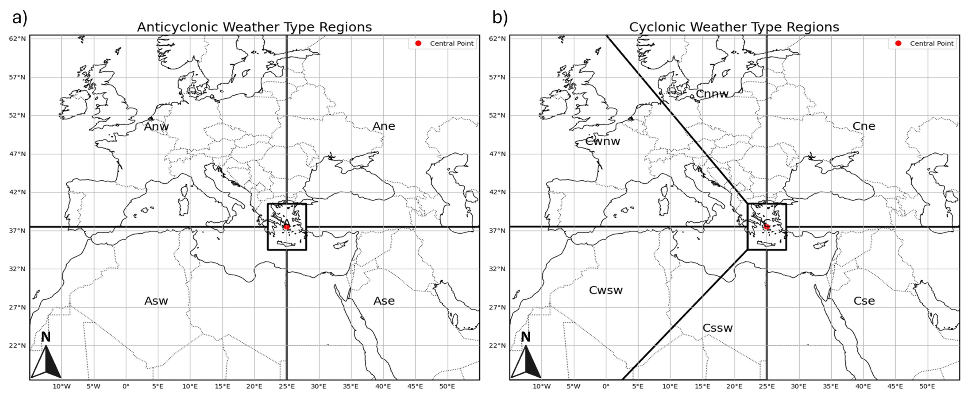
2.2. Classification of Weather Types

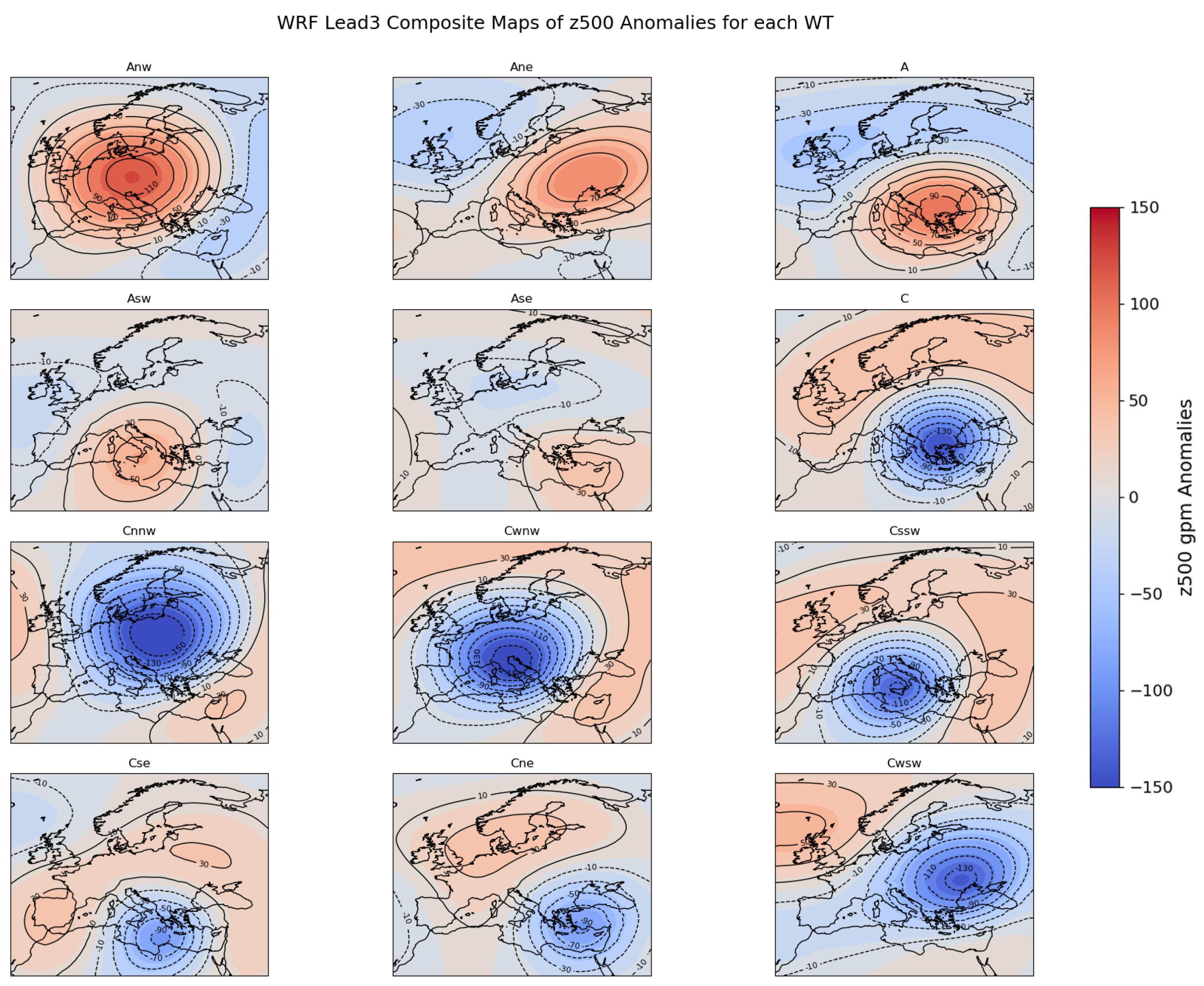
In order to create a calendar for weather types, an updated version of the one developed by [36] was implemented. The method classifies synoptic weather types based on the geopotential height at a 500 hPa surface. To perform the classification, we followed the steps described in [36]. Initially, the central point is selected, which corresponds to the area of interest. To represent the Eastern Mediterranean, a reference point over Greece (39.5° N, 25° E) was defined. Next, normalized z500 daily anomalies of the 500 hPa geopotential height (z500) were calculated using the 1981–2000 as the climatological reference period. The initial step in weather type classification involves defining the prevailing synoptic condition over the area of interest (cyclonic or anticyclonic). In characterizing the condition as cyclonic or anticyclonic, earlier methods used the anomaly sign in a $3\times 3$ sub-grid centered on the region. To classify each day, the daily average anomaly over the region is examined. A negative anomaly indicates a cyclonic day, while a positive anomaly indicates an anticyclonic day. The key improvement in this classification method is the inclusion of vertical velocity ($\omega$) along with the 500 hPa geopotential field. This additional parameter helps to better identify the atmospheric condition, especially when the 500 hPa anomaly is close to zero. For the same $3\times 3$ sub-area, the daily mean vertical velocity is calculated. If the geopotential height anomaly lies within ±1 standard deviation—indicating no significant deviation from the climatological mean, then the classification relies on $\omega$. In such cases, dominant upward motion (negative $\omega$ values) suggests cyclonic conditions, while dominant downward motions (positive $\omega$ values) indicate anticyclonic conditions. This addition improves classification accuracy by considering not only the 500 hPa level but also the vertical movement of the air masses. Based on the location of the center, the classification method identifies twelve circulation types, five anticyclonic (Anw, Ane, A, Asw, Ase) and seven cyclonic (C, Cnnw, Cwnw, Cwsw, Cssw, Cse, Cne). The weather type locations for the present study are shown in Figure 2.

The classification was performed in both ERA5 reanalysis data [37] and WRF seasonal forecasts, using z500 geopotential height and vertical velocity fields. For seasonal data, WRF hindcasts with a lead time of 3 were used, meaning that each month is simulated with initial conditions three months in advance.

3. Results

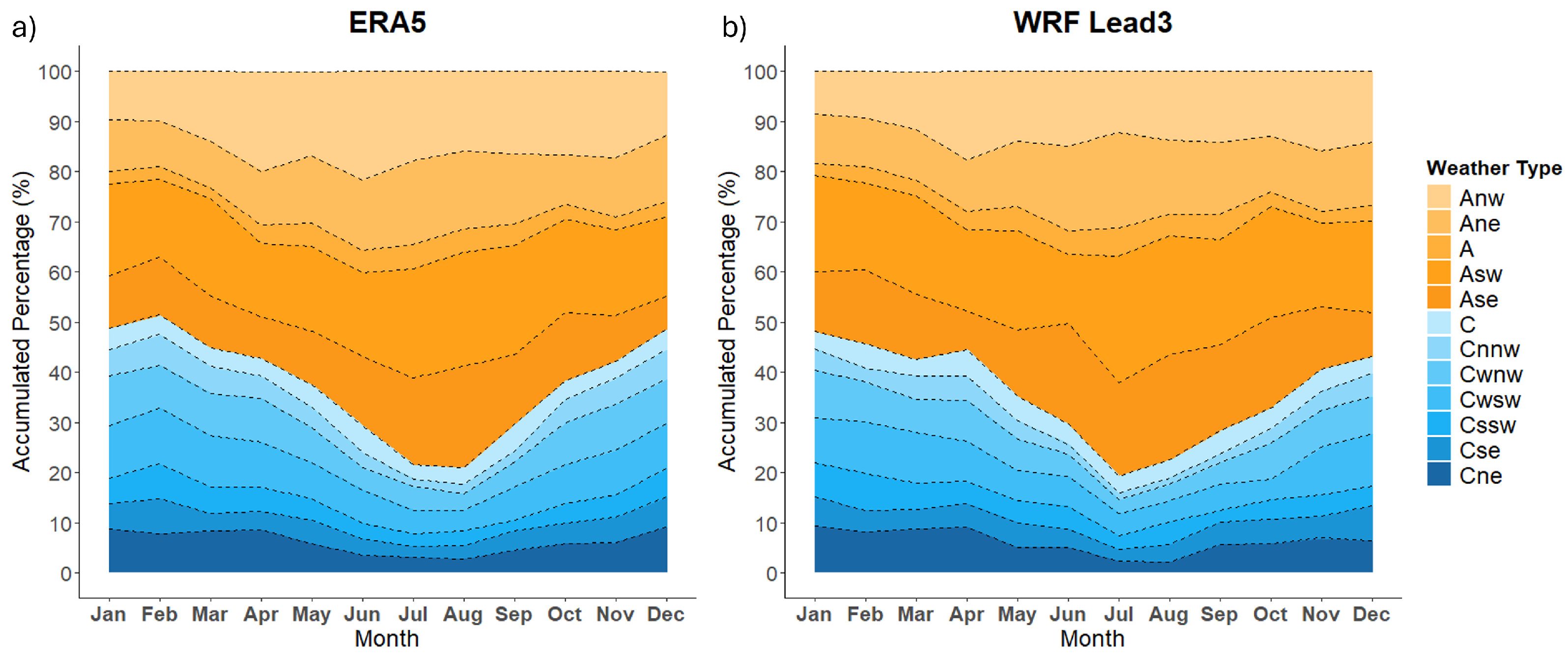
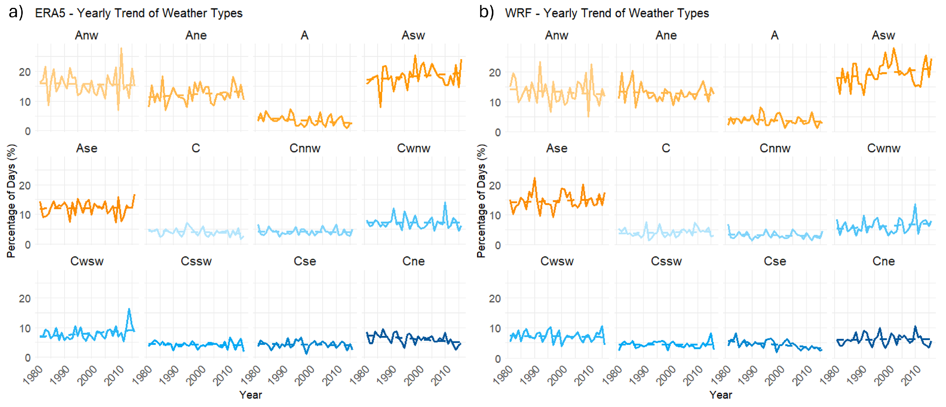
3.1. Climate Analysis of Weather Types

The classification of weather types has been applied for the z500 field and for the period 1981–2016 for both ERA5 reanalysis [37] and seasonal data. In Figure 3, the composite of z500 anomalies of each of the 12 weather types is shown for the selected period (1981–2016). Contours are used for better identification of each center position. It is obvious that cyclonic types are associated with more intense anomalies. Regarding teleconnection patterns, the anticyclonic types Ane, Anw, and A, are present with a positive phase of NAO, characterized by negative anomalies over Iceland and positive over the Azores. In contrast, the cyclonic types Cnnw (7), Cwnw (8), and especially Cne (12) are linked to the negative phase of the NAO, with the z500 field having the opposite sign. The mean z500 anomalies for the WRF hindcasts at a lead time of 3 are also presented in Figure 4. It is clear that in the WRF model, the simulated anomalies are larger than in those from the ERA5 and the centers are better established. Again, the anticyclonic types Asw and Ase present the lowest values, while the most intense anomalies are for the cyclonic types C, Cnnw, and Cwnw.

Figure 5a,b show the monthly percentage of occurrence for each of the twelve weather types based on reanalysis data and WRF model output, respectively. In both figures, anticyclonic types are shown in orange and cyclonic types in blue. The exact percentages of the circulation regimes and WTs from both ERA5 and WRF-Lead3 can be found in Tables S3–S6. Overall, 64.1% of the days are classified as anticyclonic compared to 62.1% in the reanalysis. A clear seasonal pattern is observed in both datasets, with anticyclonic types dominating during the summer months. In the reanalysis data (Figure 5a and Table S3), anticyclonic types account for 71% of cases in June, 78% in July, and 79% in August, while the WRF output (Figure 5b and Table S4) shows similar values of 70.3%, 80.6%, and 77.6%, respectively. During the winter months, differences between the two datasets become more apparent. In the reanalysis data, anticyclonic and cyclonic types occur with nearly equal frequency in December and January (51.3% anticyclonic vs. 48.7% cyclonic), with February being the only month in which cyclonic types slightly dominate (51.3%). In contrast, the WRF simulations display a higher frequency of anticyclonic types throughout winter, with 56.9% in December, 51.9% in January, and 54.4% in February.

Throughout the year, both datasets indicate that the most frequent weather types are the anticyclonic Asw and Ase, followed by Anw and Ane. The highest occurrence in the reanalysis (Table S5) is for type Asw (4) in August (22.9%), whereas in the WRF data (Table S6), it peaks in July (25.4%). Among cyclonic types, those located in the western part of the domain (Cwnw and Cwsw) are the most common, which aligns with the frequent development of cyclones in the Gulf of Genoa. In contrast, types centered over the core region of the classification domain—namely A and C for anticyclonic and cyclonic types, respectively—have the lowest frequency of occurrence. This is mainly because these types represent a relatively small spatial area, which significantly reduces the likelihood that a synoptic system will be centered directly over the region of interest.

The linear trends of each one of the classified weather types from both the reanalysis data (Figure 6a) and WRF lead time 3 hindcast (Figure 6b) have been calculated. To test the significance of the trends, a two-sided t-test was performed [40]. Most of the observed trends are not statistically significant in the 0.05 level (Table S7a), indicating no notable long-term changes in the overall frequency of occurrence during the historical period (1981–2016). A statistically significant decreasing trend is observed only for the cyclonic type 12 (Cne) and anticyclonic type 3 (A) in ERA5. Similar to the reanalysis data, the WRF-Lead3 Seasonal data (Figure 6b) also show no statistically significant trends overall (Table S7b). Only Weather Type 11 (Cse) exhibits a significant decreasing trend during the period 1981–2016. When comparing the trends between WRF and ERA5, there is a clear agreement in the classifications, with each weather type displaying comparable percentages. Trends for each WT were also calculated separately for each season (Figures S1 and S2), further supporting the agreement between WRF-Lead3 and ERA5 classifications, although most seasonal trends remain statistically non-significant (Tables S8 and S9).

3.2. WT Classification Agreement Between WRF Lead Time 3 and ERA5

Table 2. Monthly percentage agreement between WRF-Lead3 and ERA5 of daily condition (anticyclonic/cyclonic).

Month	Mean Agreement (%)	Max Agreement (%)	Min Agreement (%)
01	82.6	96.8	71
02	80.6	100	57.1
03	79.7	96.8	58.1
04	78.7	96.7	63.3
05	76.3	93.6	51.6
06	76.1	93.3	36.7
07	80.3	100	51.6
08	81	100	61.3
09	78.8	96.7	60
10	78.1	90.3	61.3
11	82	96.7	63.3
12	80.1	93.6	54.8

and

Table 3. Monthly percentage agreement between WRF-Lead3 and ERA5 on daily weather type.

Month	Mean Agreement (%)	Max Agreement (%)	Min Agreement (%)
01	49.1	64.5	25.8
02	47.8	65.5	21.2
03	45.3	64.5	16.1
04	43.6	63.3	26.7
05	37.7	61.3	19.4
06	37.1	56.7	16.7
07	39.8	71	19.4
08	38.6	64.5	16.1
09	38.9	56.7	23.3
10	43.3	67.7	19.4
11	46.9	76.7	26.7
12	45.2	67.7	22.6

present the monthly agreement between the WRF-Lead3 seasonal forecast and ERA5 reanalysis data in terms of synoptic circulation patterns and specific weather types over Greece, evaluated three months in advance.

In Table 2, the agreement refers to the day-to-day classification of general circulation conditions as anticyclonic or cyclonic. On average, the WRF-Lead3 achieves a notable 80% agreement in monthly values ranging from 76.1% in June to 82.6% in January. Maximum daily agreement has reached up to 100% in some months (e.g., February, July, and August), while the lowest minimum agreement drops to 36.7% in June, highlighting more variability during summer. These results indicate a strong ability of the model to capture the prevailing synoptic scale regime three months in advance, especially in winter.

Table 3 assessed the model’s performance in reproducing the specific daily weather type as defined by the established classification. The average agreement for this more detailed categorization is approximately 43% across the year. Agreement varies considerably by month, with November reaching up to 76.7% on individual days and March and August showing minimum daily agreement as low as 16.1%. Although daily weather types are not the primary target of seasonal forecasts, this level of agreement is still meaningful and suggests that the model retains some skill in capturing fine-scale atmospheric variability. Seasonal forecast models like WRF-Lead3 are not designed to predict specific day-to-day weather patterns months in advance. Therefore, achieving 50% accuracy for daily weather types and 80% for general circulation conditions is a strong indication of the model’s predictive capability, especially during the winter months, when synoptic patterns tend to be more stable and better constrained by large-scale dynamics.

4. Discussion and Conclusions

Seasonal forecasts provide critical insights into large-scale atmospheric variability several months in advance, serving as a valuable tool for early-warning systems and strategic planning in sectors such as agriculture, water resource management, tourism, health, and disaster risk reduction. Despite substantial progress in global seasonal forecasting systems, considerable challenges remain—particularly in accurately representing synoptic-scale atmospheric patterns, which are essential for understanding regional climate variability and extremes. To address these gaps and improve regional forecasts over the Mediterranean, this study implemented a dynamically downscaled seasonal forecasting system over the Eastern Mediterranean using the Advanced Research WRF (WRF-ARW) model.

The system was evaluated through a set of seasonal hindcast experiments at a three-month lead time, focusing on the simulation of large-scale synoptic features. A key methodological advancement of this work was the application of a refined weather type classification system, based on 500 hPa geopotential height and vertical velocity fields, which allowed for the objective identification of dominant circulation regime patterns over the Southeastern Mediterranean. This classification was applied consistently to both ERA5 reanalysis and WRF-Lead3.

Although this study does not directly examine teleconnections, it is worth noting that the Eastern Mediterranean region is influenced by several modes of climate variability, including the North Atlantic Oscillation (NAO), the East Atlantic/Western Russia (EAWR) pattern, and occasionally by ENSO. ENSO has a significant impact on seasonal forecasts in the Eastern Mediterranean, influencing weather types such as the Red Sea Trough and Cyprus Lows [41]. The teleconnections between ENSO and the Eastern Mediterranean are complex and involve large-scale atmospheric pathways such as Rossby wave trains [42,43] and the NAO [44]. However, the non-stationary nature of these teleconnections and model limitations pose challenges for seasonal predictability. Further research is needed to address these challenges and improve the representation of ENSO-related climate variability in forecasting models. These large-scale drivers can modulate the frequency and persistence of synoptic weather types, and their influence on model performance could be addressed in future studies.

The results showed that the WRF model successfully reproduced the dominant synoptic circulation types, with approximately 80% agreement in classifying daily conditions as cyclonic or anticyclonic. Notably, this agreement was stronger during winter, when large-scale atmospheric patterns are more stable and predictable due to the enhanced influence of planetary waves and baroclinic activity. While the model’s performance in predicting specific daily weather types was understandably lower (mean agreement almost 50%), this level of skill remains significant, especially considering the long lead time and the inherently chaotic nature of the atmosphere at synoptic scales.

The analysis of the monthly frequency confirmed a strong seasonal signal, with anticyclonic types dominating in summer. This seasonal transition reflects the northward shift of Hadley Cell [45,46,47] and the increased subsidence over the subtropics, particularly evident in the frequent occurrence of the southern anticyclonic types Asw and Ase during warm months. In contrast, winter months displayed a more balanced distribution of anticyclonic and cyclonic types in ERA5, while the WRF model slightly overestimated anticyclonic conditions—potentially due to biases in the representation of cloud-radiative feedback or storm track positioning. Although some earlier studies based on z500 anomalies [36] and self-organizing map classifications [48] suggested a higher frequency of cyclonic types—particularly during winter—these differences are not substantial. Those studies also identified an increasing trend in anticyclonic conditions toward the end of the 20th century. Given that nearly two decades have passed since then, it is reasonable that anticyclonic types now dominate the circulation in the Eastern Mediterranean, as confirmed by both the ERA5 reanalysis and the WRF simulations in this study.

Trends derived from ERA5 suggest a slight but non-significant increase in anticyclonic conditions over recent decades, pointing to a possible shift toward more stable weather regimes. This may be associated with increased drought frequency and intensity, as well as higher summer temperatures, thus exacerbating the risk of heatwaves in the region. Of particular note is the observed increase in the Ane weather type during summer, which is linked to the Etesian winds [49,50]—a persistent northerly flow that plays a key role in modulating heat and moisture over Eastern Mediterranean. This increase aligns with recent studies that indicate a lengthening of Etesian duration under 21st century climate projections, potentially influenced by the strengthening of the subtropical ridge and modification in land–sea thermal contrast [51,52].

These findings underline the added value of integrating a synoptic scale classification system into a seasonal forecasting approach. They demonstrate that high-resolution regional models like WRF, when carefully calibrated and downscaled from global seasonal predictors, can provide meaningful and physically consistent long-range guidance. This capability is particularly relevant for climate-sensitive regions like the Mediterranean, where seasonal anomalies can have profound socioeconomic impacts. Future work will explore the sensitivity of predictability to different lead times, as well as the comparative performance of WRF against state-of-the-art global systems, such as ECMWF SEAS5, to further validate and optimize its predictive capabilities.

References

1. Intergovernmental Panel on Climate Change (IPCC). Climate Change 2021—The Physical Science Basis; Cambridge University Press: Cambridge, UK, 2023. [Google Scholar] [CrossRef]
2. Diffenbaugh, N.S.; Burke, M. Global warming has increased global economic inequality. Proc. Natl. Acad. Sci. USA 2019, 116, 9808–9813. [Google Scholar] [CrossRef] [PubMed]
3. Lazoglou, G.; Papadopoulos-Zachos, A.; Georgiades, P.; Zittis, G.; Velikou, K.; Manios, E.M.; Anagnostopoulou, C. Identification of climate change hotspots in the Mediterranean. Sci. Rep. 2024, 14, 29817. [Google Scholar] [CrossRef] [PubMed]
4. Lionello, P.; Scarascia, L. The relation between climate change in the Mediterranean region and global warming. Reg. Environ. Change 2018, 18, 1481–1493. [Google Scholar] [CrossRef]
5. Giorgi, F. Climate change hot-spots. Geophys. Res. Lett. 2006, 33. [Google Scholar] [CrossRef]
6. Tramblay, Y.; Koutroulis, A.; Samaniego, L.; Vicente-Serrano, S.M.; Volaire, F.; Boone, A.; Page, M.L.; Llasat, M.C.; Albergel, C.; Burak, S.; et al. Challenges for drought assessment in the Mediterranean region under future climate scenarios. Earth-Sci. Rev. 2020, 210, 103348. [Google Scholar] [CrossRef]
7. Manzanas, R.; Torralba, V.; Lledó, L.; Bretonnière, P.A. On the Reliability of Global Seasonal Forecasts: Sensitivity to Ensemble Size, Hindcast Length and Region Definition. Geophys. Res. Lett. 2022, 49, e2021GL094662. [Google Scholar] [CrossRef]
8. Portele, T.C.; Lorenz, C.; Dibrani, B.; Laux, P.; Bliefernicht, J.; Kunstmann, H. Seasonal forecasts offer economic benefit for hydrological decision making in semi-arid regions. Sci. Rep. 2021, 11, 10581. [Google Scholar] [CrossRef]
9. Soares, M.B.; Daly, M.; Dessai, S. Assessing the value of seasonal climate forecasts for decision-making. Adv. Rev. 2018, 9, e523. [Google Scholar] [CrossRef]
10. Bauer, P.; Thorpe, A.; Brunet, G. The quiet revolution of numerical weather prediction. Nature 2015, 525, 47–55. [Google Scholar] [CrossRef]
11. Zhang, F.; Sun, Y.Q.; Magnusson, L.; Buizza, R.; Lin, S.J.; Chen, J.H.; Emanuel, K. What is the predictability limit of midlatitude weather? J. Atmos. Sci. 2019, 76, 1077–1091. [Google Scholar] [CrossRef]
12. Kirtman, B.; Power, S.B.; Adedoyin, A.J.; Boer, G.J.; Bojariu, R.; Camilloni, I.; Doblas-Reyes, F.; Fiore, A.M.; Kimoto, M.; Meehl, G.; et al. Near-term climate change: Projections and predictability. In Climate Change 2013 the Physical Science Basis: Working Group I Contribution to the Fifth Assessment Report of the Intergovernmental Panel on Climate Change; Cambridge University Press: Cambridge, UK, 2013; Volume 9781107057999. [Google Scholar] [CrossRef]
13. Vitart, F.; Robertson, A.W. The sub-seasonal to seasonal prediction project (S2S) and the prediction of extreme events. NPJ Clim. Atmos. Sci. 2018, 1, 3. [Google Scholar] [CrossRef]
14. Mariotti, A.; Ruti, P.M.; Rixen, M. Progress in subseasonal to seasonal prediction through a joint weather and climate community effort. NPJ Clim. Atmos. Sci. 2018, 1, 4. [Google Scholar] [CrossRef]
15. Palmer, T.N.; Anderson, D.L. The prospects for seasonal forecasting—A review paper. Q. J. R. Meteorol. Soc. 1994, 120, 755–793. [Google Scholar] [CrossRef]
16. Barnston, A.G.; Glantz, M.H.; He, Y. Predictive skill of statistical and dynamical climate models in SST forecasts during the 1997–1998 El Niño episode and the 1998 La Niña onset. Bull. Am. Meteorol. Soc. 1999, 80, 217–244. [Google Scholar] [CrossRef]
17. Doblas-Reyes, F.J.; García-Serrano, J.; Lienert, F.; Biescas, A.P.; Rodrigues, L.R. Seasonal climate predictability and forecasting: Status and prospects. Wiley Interdiscip. Rev. Clim. Change 2013, 4, 245–268. [Google Scholar] [CrossRef]
18. Lenssen, N.J.; Goddard, L.; Mason, S. Seasonal forecast skill of enso teleconnection maps. Weather Forecast. 2020, 35, 2387–2406. [Google Scholar] [CrossRef]
19. Klemm, T.; McPherson, R.A. The development of seasonal climate forecasting for agricultural producers. Agric. For. Meteorol. 2017, 232, 384–399. [Google Scholar] [CrossRef]
20. Ceglar, A.; Toreti, A. Seasonal climate forecast can inform the European agricultural sector well in advance of harvesting. NPJ Clim. Atmos. Sci. 2021, 4, 42. [Google Scholar] [CrossRef]
21. Clark, R.T.; Bett, P.E.; Thornton, H.E.; Scaife, A.A. Skilful seasonal predictions for the European energy industry. Environ. Res. Lett. 2017, 12, 024002. [Google Scholar] [CrossRef]
22. Torralba, V.; Doblas-Reyes, F.J.; MacLeod, D.; Christel, I.; Davis, M. Seasonal climate prediction: A new source of information for the management of wind energy resources. J. Appl. Meteorol. Climatol. 2017, 56, 1231–1247. [Google Scholar] [CrossRef]
23. Cai, X.; Cao, H.; Fang, X.; Sun, J.; Yu, Y. A View for Atmospheric Unpredictability. Front. Earth Sci. 2021, 9. [Google Scholar] [CrossRef]
24. Juricke, S.; MacLeod, D.; Weisheimer, A.; Zanna, L.; Palmer, T.N. Seasonal to annual ocean forecasting skill and the role of model and observational uncertainty. Q. J. R. Meteorol. Soc. 2018, 144, 1947–1964. [Google Scholar] [CrossRef]
25. He, X.; Li, Y.; Liu, S.; Xu, T.; Chen, F.; Li, Z.; Zhang, Z.; Liu, R.; Song, L.; Xu, Z.; et al. Improving regional climate simulations based on a hybrid data assimilation and machine learning method. Hydrol. Earth Syst. Sci. 2023, 27, 1583–1606. [Google Scholar] [CrossRef]
26. Merryfield, W.J.; Baehr, J.; Batté, L.; Becker, E.J.; Butler, A.H.; Coelho, C.A.; Danabasoglu, G.; Dirmeyer, P.A.; Doblas-Reyes, F.J.; Domeisen, D.I.; et al. Current and emerging developments in subseasonal to decadal prediction. Bull. Am. Meteorol. Soc. 2020, 101, E869–E896. [Google Scholar] [CrossRef]
27. Dayan, U.; Tubi, A.; Levy, I. On the importance of synoptic classification methods with respect to environmental phenomena. Int. J. Climatol. 2012, 32, 681–694. [Google Scholar] [CrossRef]
28. Bissolli, P.; Dittmann, E. The objective weather type classification of the German weather service and its possibilities of application to environmental and meteorological investigations. Meteorol. Z. 2001, 10, 253–260. [Google Scholar] [CrossRef]
29. Lamb, H.H. British Isles Weather Types and a Register of the Daily Sequence of Circulation Patterns, 1861–1971; H.M. Stationery Office: London, UK, 1972; Volume 16, Issue 116 of Geophysical Memoirs. [Google Scholar]
30. Su, S.H.; Chu, J.L.; Yo, T.S.; Lin, L.Y. Identification of synoptic weather types over Taiwan area with multiple classifiers. Atmos. Sci. Lett. 2018, 19, e861. [Google Scholar] [CrossRef]
31. Philipp, A.; Bartholy, J.; Beck, C.; Erpicum, M.; Esteban, P.; Fettweis, X.; Huth, R.; James, P.; Jourdain, S.; Kreienkamp, F.; et al. Cost733cat—A database of weather and circulation type classifications. Phys. Chem. Earth 2010, 35, 360–373. [Google Scholar] [CrossRef]
32. Neal, R.; Fereday, D.; Crocker, R.; Comer, R.E. A flexible approach to defining weather patterns and their application in weather forecasting over Europe. Meteorol. Appl. 2016, 23, 389–400. [Google Scholar] [CrossRef]
33. Piotrowicz, K.; Ciaranek, D. A selection of weather type classification systems and examples of their application. Theor. Appl. Climatol. 2020, 140, 719–730. [Google Scholar] [CrossRef]
34. Littmann, T. An empirical classification of weather types in the Mediterranean Basin and their interrelation with rainfall. Theor. Appl. Climatol. 2000, 66, 161–171. [Google Scholar] [CrossRef]
35. Maheras, P.; Patrikas, I.; Karacostas, T.; Anagnostopoulou, C. Automatic classification of circulation types in Greece: Methodology, description, frequency, variability and trend analysis. Theor. Appl. Climatol. 2000, 67, 205–223. [Google Scholar] [CrossRef]
36. Anagnostopoulou, C.; Tolika, K.; Maheras, P. Classification of circulation types: A new flexible automated approach applicable to NCEP and GCM datasets. Theor. Appl. Climatol. 2009, 96, 3–15. [Google Scholar] [CrossRef]
37. Hersbach, H.; Bell, B.; Berrisford, P.; Hirahara, S.; Horányi, A.; Muñoz-Sabater, J.; Nicolas, J.; Peubey, C.; Radu, R.; Schepers, D.; et al. The ERA5 global reanalysis. Q. J. R. Meteorol. Soc. 2020, 146, 1999–2049. [Google Scholar] [CrossRef]
38. Skamarock, W.; Klemp, J.; Dudhia, J.; Gill, D.O.; Liu, Z.; Berner, J.; Wang, W.; Powers, J.G.; Duda, M.G.; Barker, D.; et al. A Description of the Advanced Research WRF Model Version 4.1; Technical Report; National Center for Atmospheric Research: Boulder, CO, USA, 2019. [Google Scholar] [CrossRef]
39. Johnson, S.J.; Stockdale, T.N.; Ferranti, L.; Balmaseda, M.A.; Molteni, F.; Magnusson, L.; Tietsche, S.; Decremer, D.; Weisheimer, A.; Balsamo, G.; et al. SEAS5: The new ECMWF seasonal forecast system. Geosci. Model Dev. 2019, 12, 1087–1117. [Google Scholar] [CrossRef]
40. Wilks, D.S. Statistical Methods in the Atmospheric Sciences, 4th ed.; Elsevier: Amsterdam, The Netherlands, 2019. [Google Scholar] [CrossRef]
41. Hochman, A.; Gildor, H. Synergistic effects of El Niño–Southern Oscillation and the Indian Ocean Dipole on Middle Eastern subseasonal precipitation variability and predictability. Q. J. R. Meteorol. Soc. 2025, 151, e4903. [Google Scholar] [CrossRef]
42. Shaman, J. The Seasonal Effects of ENSO on Atmospheric Conditions Associated with European Precipitation: Model Simulations of Seasonal Teleconnections. J. Clim. 2014, 27, 1010–1028. [Google Scholar] [CrossRef]
43. Molteni, F.; Brookshaw, A. Early- and late-winter ENSO teleconnections to the Euro-Atlantic region in state-of-the-art seasonal forecasting systems. Clim. Dyn. 2023, 61, 2673–2692. [Google Scholar] [CrossRef]
44. Yavuzsoy-Keven, E.; Ezber, Y.; Sen, O.L. Comparative Evaluation of Niño1+2 and Niño3.4 Indices in Terms of ENSO Effects Over the Euro-Mediterranean Region. Int. J. Climatol. 2024, 44, 5839–5856. [Google Scholar] [CrossRef]
45. Zhang, G.; Wang, Z. Interannual variability of the atlantic hadley circulation in boreal summer and its impacts on tropical cyclone activity. J. Clim. 2013, 26, 8529–8544. [Google Scholar] [CrossRef]
46. Xian, T.; Xia, J.; Wei, W.; Zhang, Z.; Wang, R.; Wang, L.P.; Ma, Y.F. Is hadley cell expanding? Atmosphere 2021, 12, 1699. [Google Scholar] [CrossRef]
47. Grise, K.M.; Davis, S.M.; Staten, P.W.; Adam, O. Regional and seasonal characteristics of the recent expansion of the tropics. J. Clim. 2018, 31, 6839–6856. [Google Scholar] [CrossRef]
48. Rousi, E.; Mimis, A.; Stamou, M.; Anagnostopoulou, C. Classification of circulation types over Eastern mediterranean using a self-organizing map approach. J. Maps 2014, 10, 232–237. [Google Scholar] [CrossRef]
49. Tyrlis, E.; Lelieveld, J. Climatology and dynamics of the summer Etesian winds over the eastern Mediterranean. J. Atmos. Sci. 2013, 70, 3374–3396. [Google Scholar] [CrossRef]
50. Dafka, S.; Xoplaki, E.; Toreti, A.; Zanis, P.; Tyrlis, E.; Zerefos, C.; Luterbacher, J. The Etesians: From observations to reanalysis. Clim. Dyn. 2016, 47, 1569–1585. [Google Scholar] [CrossRef]
51. Anagnostopoulou, C.; Zanis, P.; Katragkou, E.; Tegoulias, I.; Tolika, K. Recent past and future patterns of the Etesian winds based on regional scale climate model simulations. Clim. Dyn. 2014, 42, 1819–1836. [Google Scholar] [CrossRef]
52. Dafka, S.; Toreti, A.; Zanis, P.; Xoplaki, E.; Luterbacher, J. Twenty-First-Century Changes in the Eastern Mediterranean Etesians and Associated Midlatitude Atmospheric Circulation. J. Geophys. Res. Atmos. 2019, 124, 12741–12754. [Google Scholar] [CrossRef]
Figure 1. Brief illustration of the methodology used for the sensitivity test and the final setup of the WRF model for hindcast simulations.
Atmosphere 16 00748 g001
Figure 2. Anticyclonic (a) and cyclonic (b) weather type locations based on the selected center.
Atmosphere 16 00748 g002
Figure 3. Composite maps of z500 anomalies for the period 1981–2016 and for each weather type.
Atmosphere 16 00748 g003
Figure 4. As in Figure 3, but for WRF hindcasts for the period 1981–2016 (Domain: D01).
Atmosphere 16 00748 g004
Figure 5. Accumulated monthly percentage (%) of each weather type. (a) For ERA5 reanalysis data and (b) for WRF lead 3 hindcast.
Atmosphere 16 00748 g005
Figure 6. Yearly percentage (%) of weather type occurrence. (a) from ERA5 reanalysis and (b) from WRF Lead3 hindcasts. Dashed lines indicate the linear trend.
Atmosphere 16 00748 g006