Article

Projection of Cloud Vertical Structure and Radiative Effects Along the South Asian Region in CMIP6 Models

by
Praneta Khardekar
1,2,
Hemantkumar S. Chaudhari
3,
Vinay Kumar
4 and
Rohini Lakshman Bhawar
2,*
1
Department of Physics, Savitribai Phule Pune University, Pune 411007, India
2
Department of Atmospheric and Space Sciences, Savitribai Phule Pune University, Pune 411007, India
3
Indian Institute of Tropical Meteorology (IITM), Pune 411008, India
4
Department of Atmospheric Science, Environmental Science and Physics, University of the Incarnate Word, San Antonio, TX 78209, USA
*
Author to whom correspondence should be addressed.
Atmosphere 2025, 16(6), 746; https://doi.org/10.3390/atmos16060746
Submission received: 25 April 2025 / Revised: 15 June 2025 / Accepted: 16 June 2025 / Published: 18 June 2025
(This article belongs to the Section Climatology)

Abstract

The evaluation of cloud distribution, properties, and their interaction with the radiation (longwave and shortwave) is of utmost importance for the proper assessment of future climate. Therefore, this study focuses on the Coupled Model Inter-Comparison Project Phase-6 (CMIP6) historical and future projections using the Shared Socio-Economic Pathways (SSPs) low- (ssp1–2.6), moderate- (ssp2–4.5), and high-emission (ssp5–8.5) scenarios along the South Asian region. For this purpose, a multi-model ensemble mean approach is employed to analyze the future projections in the low-, mid-, and high-emission scenarios. The cloud water content and cloud ice content in the CMIP6 models show an increase in upper and lower troposphere simultaneously in future projections as compared to ERA5 and historical projections. The longwave and shortwave cloud radiative effects at the top of the atmosphere are examined, as they offer a global perspective on radiation changes that influence atmospheric circulation and climate variability. The longwave cloud radiative effect (44.14 W/m2) and the shortwave cloud radiative effect (−73.43 W/m2) likely indicate an increase in cloud albedo. Similarly, there is an expansion of Hadley circulation (intensified subsidence) towards poleward, indicating the shifting of subtropical high-pressure zones, which can influence regional monsoon dynamics and cloud distributions. The impact of future projections on the tropospheric temperature (200–600 hPa) is studied, which seems to become more concentrated along the Tibetan Plateau in the moderate- and high-emission scenarios. This increase in the tropospheric temperature at 200–600 hPa reduces atmospheric stability, allowing stronger convection. Hence, the strengthening of convective activities may be favorable in future climate conditions. Thus, the correct representation of the model physics, cloud-radiative feedback, and the large-scale circulation that drives the Indian Summer Monsoon (ISM) is of critical importance in Coupled General Circulation Models (GCMs).

1. Introduction

The Indian Summer Monsoon is a vital aspect of life in India [1]. The variability in Indian Summer Monsoon Rainfall (ISMR) significantly influences socio-economic growth, with approximately 80% of India’s annual rainfall occurring during the summer monsoon season (June–September). As a large-scale phenomenon, the monsoon is interconnected with various global circulation systems. However, the influence of cloud properties on the Indian Summer Monsoon (ISM) remains poorly understood. The study by [2] highlights that the ISM is closely tied to the seasonal migration of the Intertropical Convergence Zone (ITCZ), which governs large-scale cloud band formation. Additionally, monsoon depressions—key synoptic-scale systems—drive strong cyclonic vorticity and upward motion over the northern Bay of Bengal, facilitating cloud buildup and intense precipitation [3]. These dynamic features play a crucial role in modulating cloud development and maintenance during the monsoon. Gaining insights into water content, cloud hydrometeor formation, latent heating, and the interplay between microphysical and dynamical processes during the ISM is crucial. Understanding the interaction between cloud properties and dynamics in regulating ISM variability is essential for improving model biases, ultimately leading to more accurate ISM rainfall predictions [4]. A realistic representation of cloud formation in general circulation models (GCMs) is a key factor in improving the depiction of ISMR. In tropical regions, upper-level clouds containing ice and mixed-phase hydrometeors play a significant role in influencing the atmospheric radiation balance [5]. GCM experiments have also found that the microphysical and dynamical processes of clouds influence the radiative processes (e.g., [6]). The representation of clouds in GCMs is a challenging task, as it results from intricate interactions among radiation, moist convection, large-scale circulation, and microphysical processes. Limitations in predictive accuracy may stem from the unrealistic parameterization of cloud processes and precipitation physics in climate models [7,8,9]. Therefore, the correct representation of precipitation has been one of the major challenges in operational GCMs. Previous studies based on observations have pointed out that microphysical properties are associated with monsoon (e.g., [10,11,12]). Consequently, [13] emphasized the need for further research on the interaction between clouds and large-scale circulation, identifying it as a “grey area” in climate science. In this view, the parameterization of microphysics has utmost importance in GCMs for the simulation of ISM [14]. Stratiform rain is closely linked to the formation of cloud condensate, particularly cloud ice and mixed-phase hydrometeors [4,15,16]. This type of precipitation significantly impacts ISMR (e.g., [17]), as satellite observations over the Indian Summer Monsoon region indicate that approximately 40–50% of rainfall events originate from the melting of ice [16], highlighting the crucial role of ice processes. A complete description of precipitation formation is a result of the interaction between heat produced by clouds and the induced circulation, a vertical structure that requires a good understanding of the characteristics and behavior of the different hydrometeors in the atmosphere.
The interaction between clouds and radiation is often described through cloud-radiative effects at the top of the atmosphere, which measure the influence of clouds by comparing Earth’s energy balance with that of a hypothetical clear-sky scenario where clouds are completely transparent to radiation. This widely used top-of-atmosphere perspective serves as the foundation for understanding cloud-radiative feedback and their role in climate sensitivity [18]. Cloud-radiative heating has been shown to influence the internal variability of the climate system to varying extents, affecting phenomena such as the Madden–Julian Oscillation [19], the El Niño–Southern Oscillation [20], and the North Atlantic Oscillation [21,22]. Additionally, it plays a crucial role in shaping the response of planetary-scale atmospheric circulation to global warming [23,24,25,26]. The annual Indian Summer Monsoon (ISM) cycle is driven by the seasonal migration of the Intertropical Convergence Zone (ITCZ), marked by a sudden onset and a deep overturning meridional circulation (regional Hadley cell) linked to latent heat release from ISM precipitation. After onset, the land surface cools, reversing the surface temperature gradient, but the tropospheric temperature (TT) gradient becomes strongly positive, sustaining the monsoon. This shift in TT gradient triggers symmetric instability, driving the northward progression of the ITCZ and offering a framework to understand ISM variability through TT influences in the north and south [27].
Climate models are crucial for projecting future climate changes. The primary goal of the Coupled Model Intercomparison Project (CMIP) is to improve the understanding of past, present, and future climate, including its variability and changes driven by both natural fluctuations and variations in radiative forcing within a multi-model framework. Across different CMIP phases, several advancements have been observed, particularly in the large-scale climatological patterns of temperature, water vapor, and zonal wind speed. Accurately evaluating clouds in global climate models is essential for assessing their ability to reproduce observed climate and project future changes. CMIP, an initiative of the World Climate Research Programme (WCRP), provides coordinated Earth System Model (ESM) simulations for historical and future climate scenarios [28]. Within CMIP6, the newly developed Scenario Model Intercomparison Project (ScenarioMIP) focuses on climate projections based on scenarios that address societal concerns related to climate change mitigation and adaptation. These projections are driven by updated emissions and land-use scenarios, covering a range of radiative forcing from low- to high-emission pathways [29,30]. Previous studies have reported significant errors in the simulation of clouds and water vapor structures in GCMs, as well as their relationship with large-scale dynamic and thermodynamic conditions, and radiation budgets in CMIP5 (e.g., [31,32]). Similarly, the challenge in predicting the Asian monsoon stems from the inability of climate models to accurately simulate the observed distribution and intensity of monsoon rainfall. Despite advancements from pre-CMIP3 to CMIP3 and CMIP5 models, significant improvements remain elusive in GCMs [33,34,35]. The studies by [4] have pointed out that the biases in cloud representation within GCMs primarily result from the inadequate depiction of ice and liquid water content profiles. In the Coupled Model Intercomparison Project Phase 6 (CMIP6), the latest generation of GCMs incorporates a higher spatial resolution (both horizontal and vertical) along with arguably more advanced model physics [36]. The latest CMIP6 models [28] generally show slight improvements over their CMIP3 and CMIP5 predecessors when compared to observations [37]. In the same context, the study by [38] points towards a better depiction of pattern correlation in representing the mean monsoon along with an increase in the precipitation in the future projection (1pctCO2). Following from [36], a study [39] analyzing the impact of future projections on monsoon and cloud levels in ssp5–8.5 was carried out. The pattern correlation coefficient (PCC) reveals a reduced OLR in future scenarios (PCC ~0.77 vs. ~0.81 historically), likely due to cloud feedback mechanisms. Based on this, the study further explored how cloud-feedback mechanisms influence the atmosphere and general circulation. In this study, we attempted the following:
(1)
A quantitative assessment of the CMIP6-simulated cloud vertical structure, viz., water content (clw) and cloud ice content (cli) followed by the cloud-radiative effects (longwave and shortwave).
(2)
Clouds not only govern radiative energy balances, but also general atmospheric circulations are maintained by them. Thus, an assessment of cloud radiation interactions and their impact on the general atmospheric planetary circulations in the present and future climate scenarios is conducted.
(3)
The tropospheric temperature is the driving force behind the general atmospheric circulation, which in turn influences the climate, and the distribution of heat and moisture across the globe; hence, this study also evaluates the tropospheric temperature along the South Asian region.

2. Datasets Used

2.1. CMIP6 Datasets

In this study, we assessed the performance of models included in the latest phase of CMIP (CMIP6 [28]) by comparing results from the historical simulations (1850–2014) and various available scenarios (period: 2015–2100). The Shared Socio-Economic Pathways considered in this paper were the SSP1–2.6, SSP2–4.5, and SSP5–8.5 scenarios, which represent the lower, mid, and higher bound of future forcing pathways. The models and their key references are listed in Table 1 [38]. We conducted simulations (r1i1p1f1) for all selected models. These models were selected based on the study performed by [38]. In that study, 10 models were found to be the best performing in the annual cycle along the Indian region (65° E-95° E; 5° N–40° N). In this study, we continued with only five of those models, as their selection was determined by the availability of the necessary variables in both historical and future CMIP6 scenarios. All model data are freely available via the Earth System Grid Federation (ESGF; https://esgf-node.llnl.gov/projects/esgf-llnl/, Last accessed on 1 February 2024). All model outputs were re-gridded into 1° × 1° latitude and longitude for a fair comparison. For the analysis presented in this paper, the variables considered included the cloud water content (clw), cloud ice content (cli), and shortwave and longwave fluxes at the top of the atmosphere for clear and all sky. Similarly, to assess the general circulation, the vertical velocity in the pressure coordinates was taken into consideration (omega = dp/dt). The tropospheric temperature is another major factor in the assessment of the ISM; hence, we evaluated TT for the various models. For the remainder of this study, we will not analyze intermodel spread in CMIP6 and will only consider the ensemble average.

2.2. Observations and Reanalysis

The European Centre for Medium-Range Weather Forecasts (ECMWF) fifth-generation reanalysis, ERA5, is the successor to the widely used ERA-Interim reanalysis [45]. In this study, ERA5 data provided by the Copernicus Climate Change Service Climate Data Store (CDS) (Copernicus Climate Change Service, 2017) were used for the variables cloud water content and cloud ice content. The dataset used for vertical pressure velocity (omega) was the National Centers for Environmental Prediction/National Center for Atmospheric Research (NCEP/NCAR) reanalysis data [46]. To compare the model-simulated tropospheric temperature (TT), the ERA5 reanalysis dataset was used. The Clouds and Earth’s Radiant Energy Systems (CERES) Energy Balanced and Filled (EBAF) dataset offers global monthly mean top-of-atmosphere (TOA) and surface longwave (LW), shortwave (SW), and net radiative fluxes under both clear-sky and all-sky conditions. In this study, we used the CERES-EBAF Ed 4.1 monthly mean data (available March 2000–present), provided on a 1° × 1° grid. To evaluate the representation from general circulation in the CMIP6 models, the vertical velocity was taken into consideration, and for this, the ERA5 (1984–2014) dataset was used. Interpolation was performed on the CMIP6 models (historical and future simulations) for the cloud water and ice content to convert them to the pressure levels of the reanalysis dataset for a fair comparison. The Multi-Model Ensemble Mean was calculated for the above-listed CMIP6 models (Table 1).
It is beyond the scope of this work to comprehensively evaluate CMIP6 cloud properties (cloud water and ice content) against satellite retrievals such as MODIS/CALIPSO/CloudSAT, as it has been performed by numerous authors. Instead, we sought to provide an additional benchmark/reference regarding future model projections and the changes versus the historical period.

3. Results and Discussion

3.1. Cloud Vertical Structure and Radiation Effect (Longwave and Shortwave)

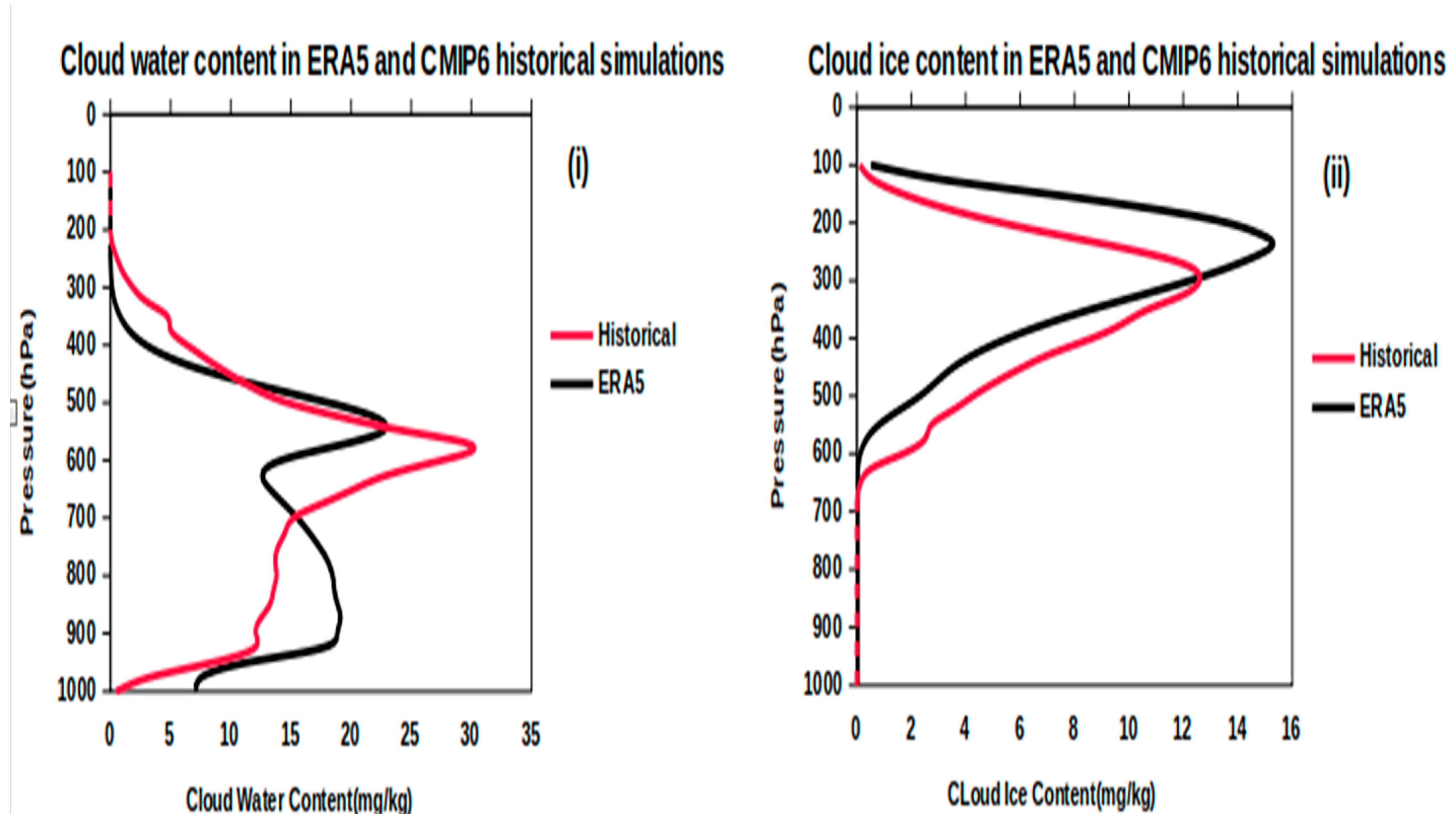
3.1.1. Historical Simulations in Cloud Water and Ice Content

The vertical extent of clouds during monsoons is governed by the large-scale monsoon circulation and moisture distribution [17]. Figure 1 depicts the spatial distribution of cloud ice content over the South Asian region (50° E–110° E, 20° S–40° N). In ERA5 (A), cloud ice is more prominently distributed over the northern Bay of Bengal. The historical simulation (B) shows an elongated concentration of cloud ice extending across the Arabian Sea, Bay of Bengal, and the Tibetan Plateau. The future scenarios align well with the historical simulation, showing an increase in cloud ice content over the Arabian Sea, particularly under the high-emission scenario (c3).
Similarly, Figure 2 shows the spatial distribution of the cloud water content over the South Asian region (50° E–110° E, 20° S–40° N). In ERA5 (A), the cloud water content is predominantly observed over the eastern part of the Tibetan Plateau and its surrounding areas. The historical simulation (B) effectively captures the cloud water distribution along the Tibetan Plateau. An increase in the cloud water content over the Arabian Sea and the Western Ghats is clearly represented in scenarios (A1–C3), which can be attributed to orographic lifting during the Indian Summer Monsoon (ISM).
Figure 3i represents the vertical structure of cloud water content in ERA5 and CMIP6 historical MME (multi-model ensemble mean) along the Indian region (65° E–95° E; 5° N–40° N). The multi-model ensemble mean seems to over-estimate the reanalysis (ERA5) in the upper and mid-troposphere. The cloud water content in historical simulations increases with a sudden jerk and reaches a value of 30 mg/kg, which is double that of the observational dataset (14.2 mg/kg). ERA5 exhibits a broad increase in the lower troposphere, which the historical simulation fails to replicate. In Figure 3ii, the cloud ice content is represented in the reanalysis (ERA5) and historical simulations. As compared to the reanalysis dataset, the MME is underestimated in the upper troposphere (400–200 hPa). In the mid-troposphere, the cloud ice content is slightly over-estimated in the reanalysis dataset. This may be due to the different convective parameterization schemes used in the models or may be due to the mixed-phase clouds in the ice content in the mid-troposphere.

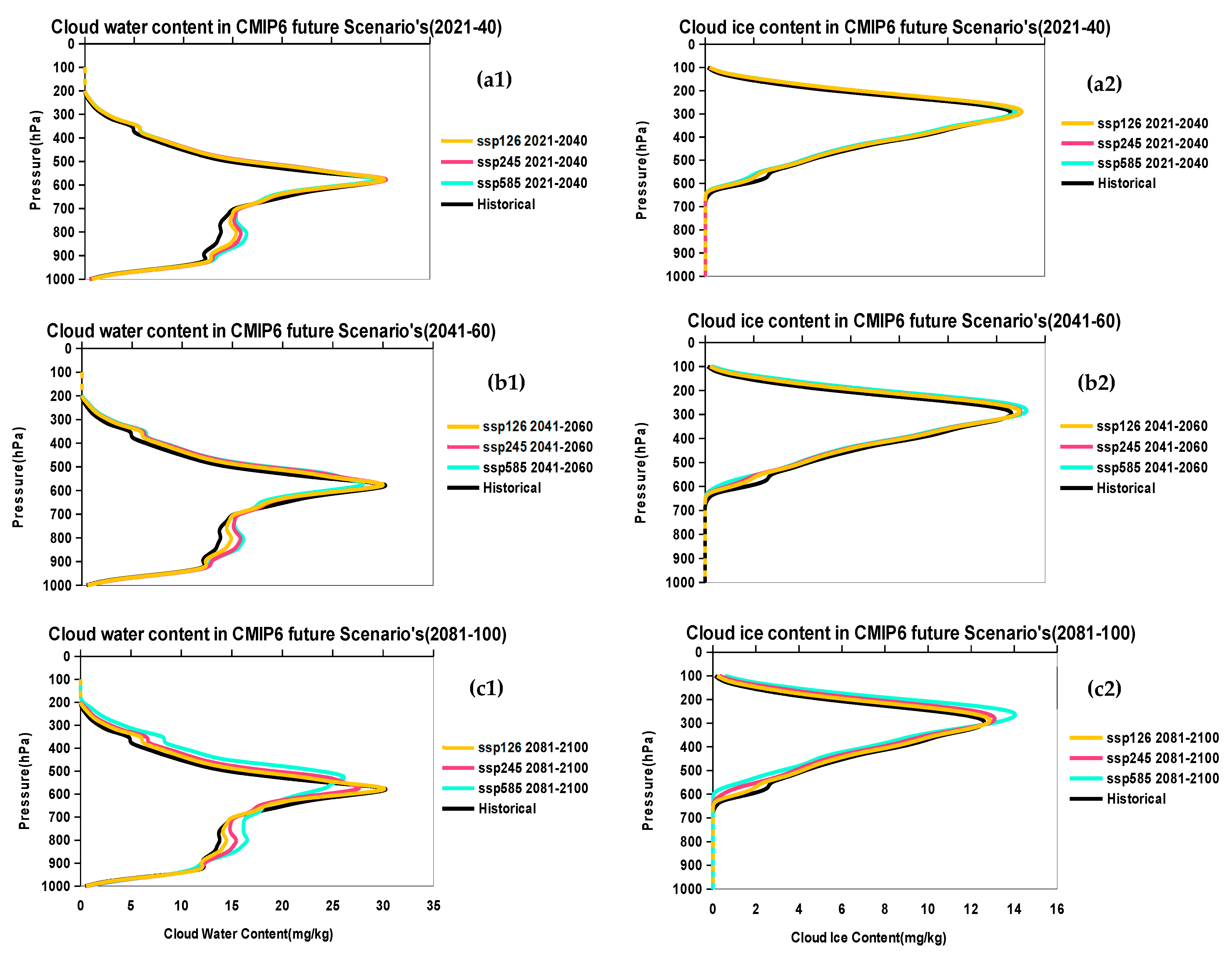
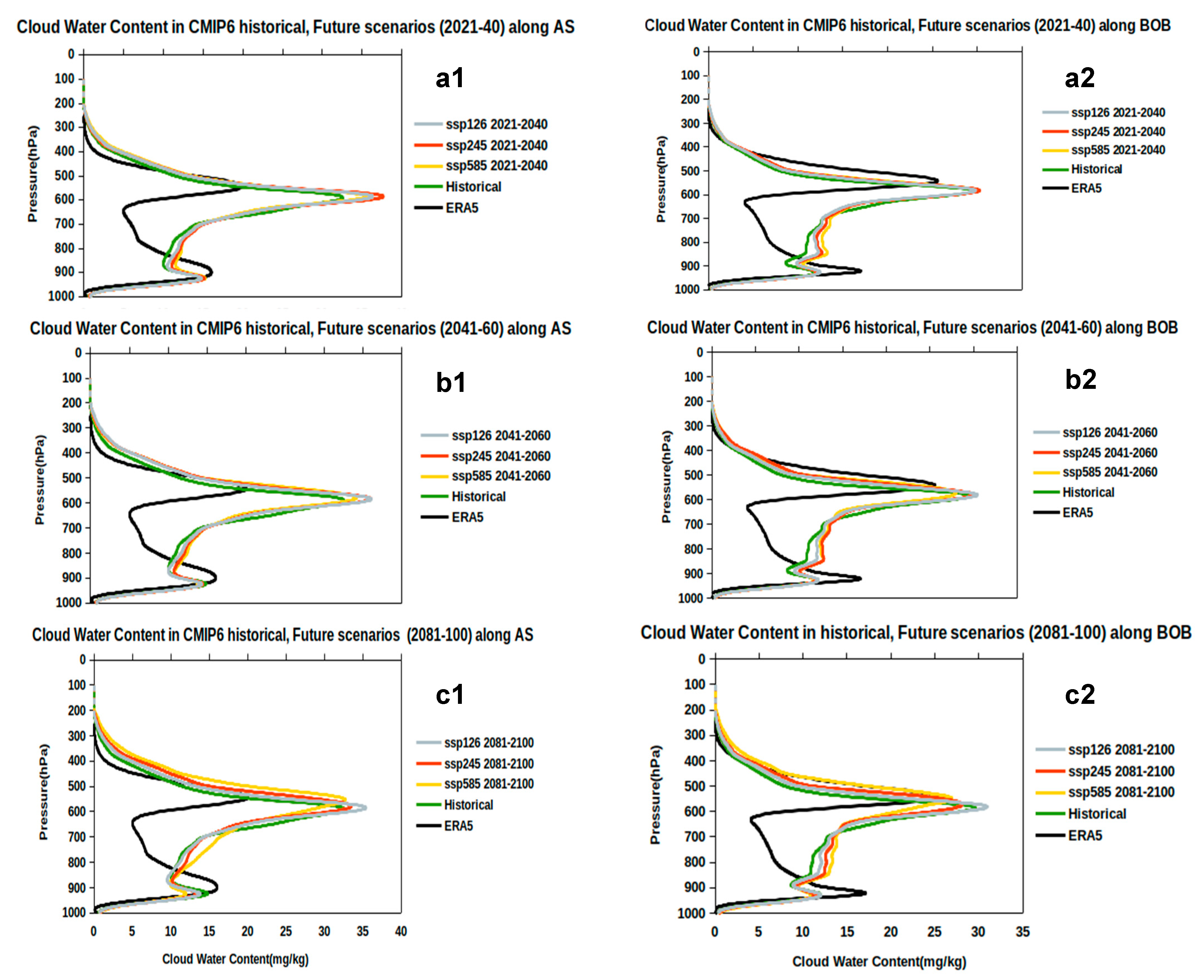
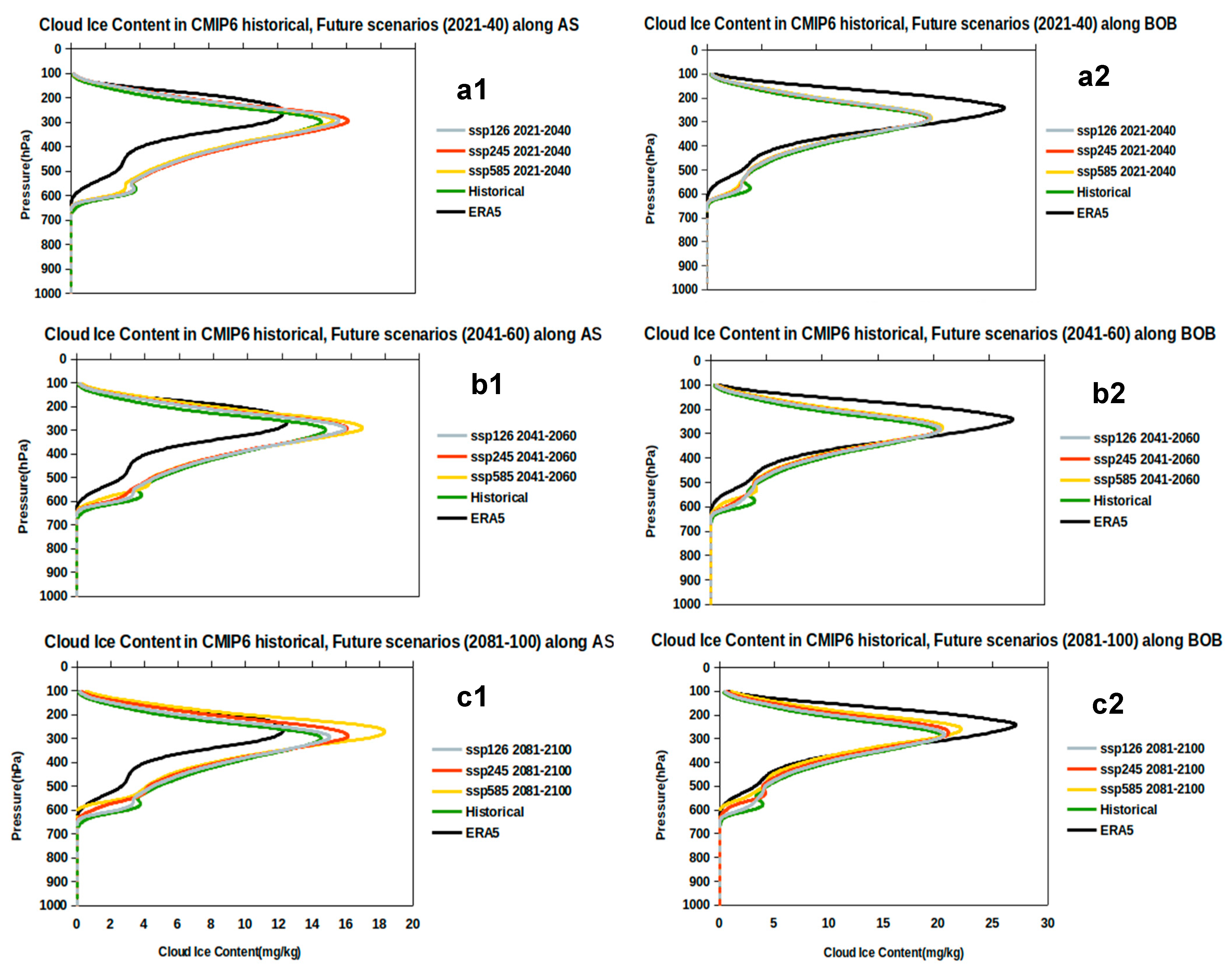
3.1.2. Future Projections

The future projections of cloud water are shown in Figure 4(a1,b1,c1), which represent the different scenarios, namely low (ssp1–2.6), moderate (ssp2–4.5), and high emission (ssp5–8.5) in near (2021–2040), mid- (2041–2060), and far future (2081–2100) years. A consistency in cloud water content is observed in the near (2021–2040) and mid-term (2041–2060) for different scenarios. An increase in the clw is noticed in the lower troposphere (all scenarios), which may be an indication of stronger monsoon circulation due to increased moisture, depending on the accurate representation of clouds in the models. A rise in the cloud water content in the troposphere (500–200 hPa) in the far future (2081–2100) under the SSP5–8.5 scenario is projected, which may lead to enhanced convective detrainment and potentially impact large-scale atmospheric dynamics, such as the Hadley circulation. Interestingly, a decrease in clw in the mid-troposphere and an increase in the lower troposphere is projected over the Indian region in the far future, compared to the low and mid-scenarios, which may influence cloud-radiative effects.
Projections of cli exhibit a similar pattern in the near (2021–2040) and mid-future (2041–2060) scenarios; however, a noticeable increase in ice content in the upper troposphere is evident, particularly in the far future (2081–2100) scenario. The increase in ice cloud may alter the radiation affecting the cloud-radiative feedback mechanism/ monsoon dynamics. Figure 5 represents the cloud water and cloud ice content along the oceanic regions (Arabian Sea and Bay of Bengal). Over the oceanic regions (Arabian Sea and Bay of Bengal), clw appears to decrease across all future scenarios within the 800–1000 hPa pressure range. Likewise, all future scenarios show a two-fold increase in clw along the mid-troposphere region (400–500 hPa), which may suggest a rise in the water vapor content
The cloud ice content along the Arabian Sea and Bay of Bengal is shown in Figure 6. In all future scenarios, the cloud ice content (cli) over the Arabian Sea shows an increase in the upper troposphere (200–400 hPa) with respect to ERA5, with the highest peak observed under the SSP5–8.5 scenario, as shown in Figure 6(a1,b1,c1). Meanwhile, over the Bay of Bengal, the future projections show a decline in cloud ice (cli) compared to the ERA5 observations.

3.2. Radiative Effects in Changing Climate

Clouds significantly influence radiative fluxes at the top of the atmosphere, as observed through satellite data, and interact with various climate system variables, as demonstrated by climate model simulations [47]. The impact of clouds on the warming or cooling of the climate system depends on various factors, including cloud-base and cloud-top height, cloud coverage, optical properties, and whether the cloud particles are in the liquid or ice phase [48]. Table 2 represents the radiative effects at the top of the atmosphere.
Uncertainties in the ice water content (IWC) and liquid water content (LWC) can affect the vertical distribution of atmospheric radiative heating. While shortwave fluxes at the top of the atmosphere (TOA) are influenced by the cloud ice content/ice water path (IWP), longwave radiation is largely governed by the temperature near the cloud top in optically thick layers, thereby reducing its dependence on the IWP distribution. The observational dataset displays an increase in the longwave cloud-radiative effect (LWCRE) along the Bay of Bengal and Central India. A similarly pronounced increase in cooling can be seen with the increase in the shortwave cloud-radiative effect (SWCRE) along Central India and the Bay of Bengal (Table 2).
In the CMIP6 multi-model mean projections, there is an increase in LWCRE under the future warming scenario (far future; ssp5–8.5) in the near future (2021–2040) as compared to the historical simulations. But the future scenarios show an increase in the SWCRE at the top of the atmosphere in all scenarios, mainly along the Oceanic region. This suggests enhanced cloud albedo, possibly due to increased high-altitude ice clouds or optically thicker clouds, which can be correlated with the statement about IWP influencing shortwave fluxes at TOA. Thus, the stronger SWCRE in future scenarios suggests increased cloud reflectivity, possibly linked to changes in the ice/liquid content.

3.3. Representation of General Circulations in CMIP6 Models/Impact of General Circulations on Clouds

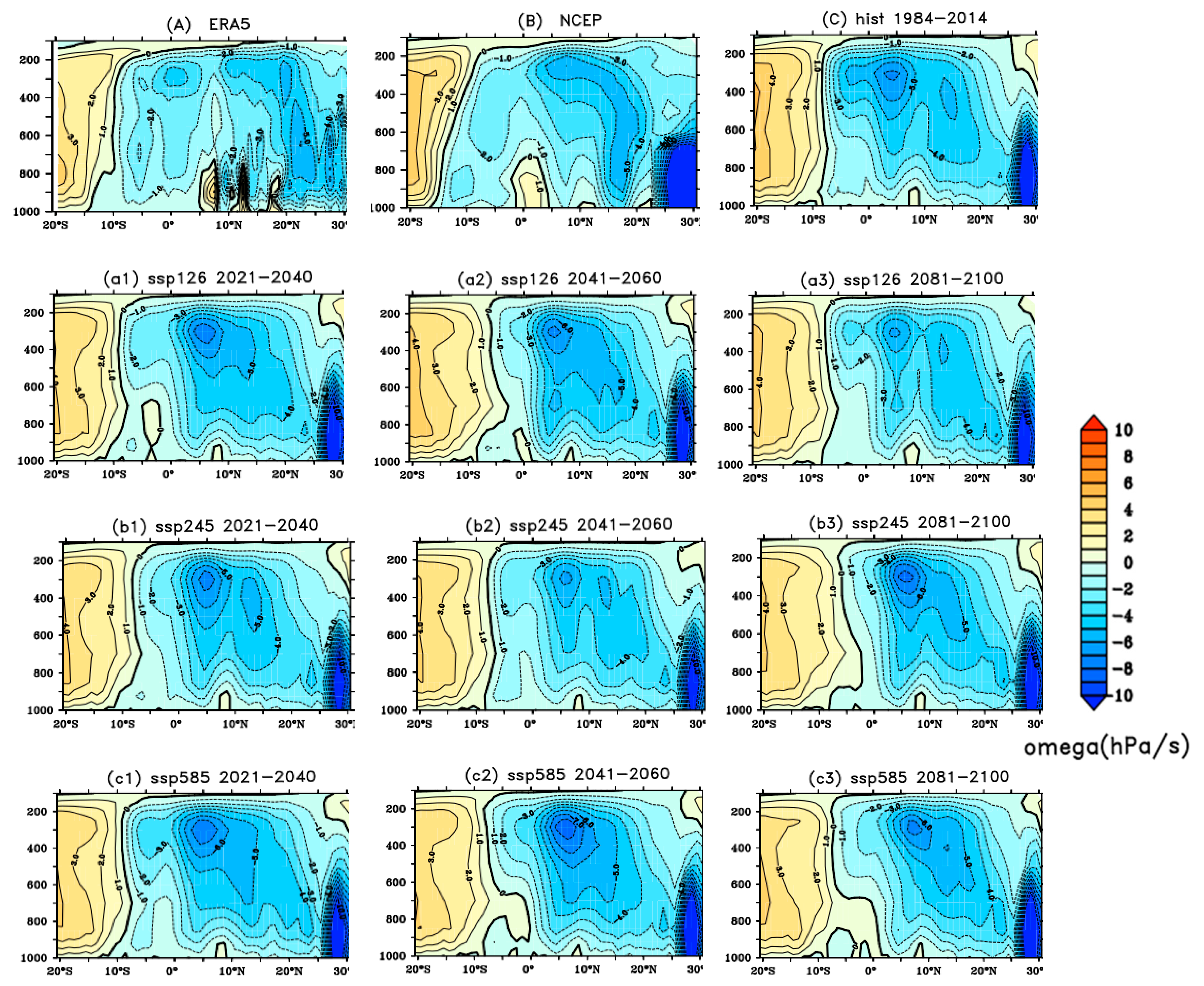
3.3.1. Hadley Circulations in Reanalysis and Historical Simulations

In the tropics, atmospheric heating associated with convection induces atmospheric convergence and divergence that drives atmospheric vertical motion and circulation. This direct circulation, comprised of zonal (Walker) and meridional (Hadley) circulations, is therefore best characterized by the divergent component of flow, more surface evaporation, and vertical motion (e.g., [49,50]). Since the vertical velocity is a proxy for the strength of dynamic disturbances [51,52,53], we evaluated the omega mean CMIP6 MME against the ERA5 and NCEP reanalysis datasets. Figure 7 represents the JJAS (June–September) meridional (Hadley) circulation averaged along the longitude (70° E–90° E) in the reanalysis ERA5 (A) and NOAA-NCEP (B) datasets and historical (C) simulations. The mean Hadley circulation exhibits a well-defined ascending branch north of 10° S and a descending branch south of 10° S. Both the reanalysis datasets show coherent regions of ascent near the Equator but with a noticeable difference in the intensity and vertical extent, signifying structural uncertainty. Notably, the ascending branch is more extensive than the descending one in both the datasets. The historical simulations exhibit a uniformly distributed ascending branch of vertical velocity that becomes more concentrated in the upper troposphere compared to the reanalysis datasets. However, simultaneously, the enhancement in the descending branch appears to extend up to 10° S, which is greater compared to both reanalysis datasets.
A prominent descending branch appears to rise from the Equator to around 5° N, whereas, in the historical simulations, it shifts closer to 10° N. The study by [54] for IPCC AR4 models argued that the overturning circulation weakens as the climate warms because surface-specific humidity increases more rapidly than precipitation with the global temperature. The reason behind this may be the increase in the warming along the Indian Ocean. Another prime factor is the representation of high clouds that cause uncertainty in the Hadley circulation intensity because ice greatly affects the radiation budget through the regulation of longwave and shortwave effects [55].

3.3.2. Historical and Future Projections

The increase in and expansion of Hadley circulation have been analyzed in various studies, which agree that the Hadley cell has expanded poleward in recent decades [56,57]. The historical simulation shown in Figure 7C indicates an intensification of the ascending branch of the Hadley cell, with the maximum concentration in the upper troposphere. The concentration in the ascending branch in low-emission scenario’s ssp1–2.6 (Figure 5(a1)) along the upper troposphere is clearly evident. Hereafter, the foci weaken in the mid- (2041–2060) and far-future (2081–2100) terms of low emission (ssp1–2.6). But the poleward shift continues in the low-emission scenario. The moderate-emission scenario SSP2–4.5 (Figure 7(b1–b3)) also exhibits an intensification of the ascending branch, accompanied by an increase in the descending branch (dry subsidence) over the Southern Hemisphere. The Hadley cell expansion in the mid-term (2041–2060) for the high-emission scenario ssp5–8.5 (Figure 7(c2)) seems to be more concentrated along the upper troposphere, with the foci center near the Equator towards 10 °N. But, in the far-future term (2081–2100) (Figure 7(c3)), the peak weakens and shifts the Hadley cell towards the pole. A previous study [56] found that there are multiple reasons behind the expansion of Hadley cell, such as increasing greenhouse gases, stratospheric ozone depletion, and anthropogenic aerosols. As SSTs warm, the Hadley cell tend to expand poleward, shifting the subtropical high-pressure systems further poleward. Additionally, warming in the Indian Ocean enhances convection, resulting in an increase in high-altitude ice clouds, as evident from Figure 6 in the future projections.

3.4. Effect of Tropospheric Temperature

3.4.1. Observational and Historical Assessment of the Tropospheric Temperature (TT)

The meridional gradient of the upper tropospheric temperature (UTT) (e.g., vertically averaged air temperature between 200 and 600 hPa) is directly related to the meridional gradient of deep tropospheric heating and can contribute to the intensification of deep tropospheric circulation [58]. The reanalysis (Figure 8A) shows a maximum in UTT along the northern part of India and the Tibetan Plateau.
Similarly, the historical simulation (Figure 8B) depicts a UTT peak over the same region but not as intense as the reanalysis.

3.4.2. Future Projections of Tropospheric Temperature

The estimation of TT in the future projections is represented in the remaining panels of Figure 8. The oceanic region in the historical simulations is the coldest one during the JJAS (June, July, August, September) as compared to the future scenarios. All CMIP6 multi-model ensemble means (a1–c2) are able to replicate the warm troposphere along the Tibetan Plateau. The low-emission scenario ssp1–2.6 (Figure 8(a1–a3)) shows a gradual warming trend. Similarly, the moderate-emission scenario ssp2–4.5 (Figure 8(b1–b3)) shows a more pronounced warming trend, particularly in the later periods (2081–2100), with TT increasing across the region. The high-emission scenario ssp5–8.5 (Figure 8(c1–c3)) shows the highest warming trend, with substantial increases in TT by the end of the century (2081–2100). With warming (especially in ssp2–4.5 (b1–b3) and ssp5–8.5 (c1–c3)), deep convective activity may increase, leading to more high clouds, particularly prevalent over the Indian Ocean and monsoon regions, where warming at these levels can enhance deep convection. A strong north–south temperature gradient (warmer land, cooler ocean) intensifies the monsoon trough and rainfall. The tropospheric temperature gradient (TTG) influences the position of the Intertropical Convergence Zone (ITCZ) and Hadley circulation. Therefore, it is crucial to study TTG. To evaluate the TTG, we computed the mean in two areas, namely a northern box (40° E–100° E, 50° N–35° N) and a southern box (40° E–100° E, 15° S–5° N), and then calculated the difference between them for every month (regions as specified in study [58]).
Figure 9 displays the TTG for the reanalysis (ERA5) and CMIP6 MME historical and future simulations. The onset of the monsoon can be estimated when the TTG changes from negative to positive. The June–September (JJAS) pattern is well captured by the reanalysis dataset. The historical simulation underestimates the TTG but is able to predict the onset and withdrawal of the monsoon along the Indian region.
Similarly, the assessment of the TTG in the future projections was analyzed. The future projections can simulate the monsoon pattern well as compared to historical simulation. An enhancement in the future scenarios can be observed, implying stronger northern warming, likely due to an intensified land–sea temperature contrast and changes in monsoon dynamics. But, in Figure 8, future projections do indicate a warmer troposphere with an almost unchanged tropospheric temperature gradient (TTG) due to proportional warming across latitudes, despite significant increases in the tropospheric temperature (TT).

3.4.3. Statistical Representation of Tropospheric Temperature

The pattern correlation between ERA5 and CMIP6 MMEs is presented over the South Asian region (40° E–110° E, 20° S–40° N) to evaluate the performance of the CMIP6 MME (Table 3). It is seen that most of the MME depicts a high correlation, above 0.95 with observation, except for SSP2–4.5 2021–2040 (0.9417). The ensembles depict a very good correlation with reanalysis (0.98) in various scenarios. This points towards the confidence of using CMIP6 MME in studying monsoon–temperature interactions and other feedback processes.
The Granger test (Table 4) was applied to assess causal links between the tropospheric temperature (TT) and cloud ice (CLI) over Central India (72° E–88° E; 18° N–28° N) during the JJAS monsoon season at lag 1. This region’s complex cloud systems can alter TT via radiative effects, while temperature changes may conversely influence cloud formation. Table 4 demonstrates bidirectional causality across all five CMIP6 models, but with notable variations: FGOALS and MPI-HR display exceptionally strong mutual feedback (F = 45.1/79.9 and 209.9/59.4), whereas NESM3 shows a weaker CLI→TT influence (F = 15.3).
Mechanistically, these results imply that warming enhances cloud ice through convection, while cloud ice modulates the temperature via radiation. Models like CMCC and MIROC6 capture this two-way coupling robustly, aligning with the observed cloud–radiation feedback in monsoons. However, MPI-HR’s extreme F-values suggest an amplified sensitivity to these processes, possibly due to high-resolution physics.
The findings emphasize the importance of accurate cloud representations in climate models. While bidirectional causality is consistent, disparities in feedback strength (e.g., NESM3′s asymmetry) reveal model-specific biases. Future work should explore nonlinear interactions and observational constraints to refine this feedback for improved monsoon predictions.
The study by [59] indicates that the CMIP6 models demonstrate an overall improvement in global SST climatology relative to CMIP5, with a transition from cold to warm biases primarily attributed to changes in radiative processes. However, the study by [60] exemplifies that significant regional SST biases persist in the Indian Ocean, which are mainly due to the misrepresentation of surface winds and ocean–atmosphere interactions. Similarly, the study by [61] pointed out that the coupled models were able to capture El Niño–Southern Oscillation Indian Summer Monsoon Rainfall (ENSO-ISMR) teleconnections more intensely as compared to atmosphere-only models, whereas, in the case of Indian Ocean Dipole ISMR teleconnections, AMIP simulations have a more pronounced impact. Including an explicit AMIP comparison in future work will clarify how warm SST biases modulate coupled model performance in SST-sensitive regions like the Indian Ocean.

4. Conclusions

One of the most considerable challenges in atmospheric science is accurately modeling cloud formation, properties, and feedback processes, as deficiencies in cloud simulations can lead to either weak or strong feedback in global climate models [62,63,64,65]. Also, clouds remain a primary source of uncertainty in representing precipitation (convective and stratiform) and radiative balances. While CMIP6 is a step forward in simulating clouds, significant uncertainties remain, and the correct or accurate depiction of the various factors by climate models needs to be addressed in the warming world [38,39]. These uncertainties continue to be a significant limitation in weather and climate forecasting, as well as in climate change simulations, highlighting the importance of understanding cloud–radiation interactions and their varied characteristics within the Earth’s atmosphere [66,67]. In reality, the relationship between the cloud amount and the cloud-radiative effect is not purely linear [68]. Also, the large-scale circulations drive the monsoon dynamics. The north–south gradient of vertically averaged air temperature between 200 and 600 hPa (referred to as tropospheric temperature (TT)) over the Indian subcontinent plays a crucial role in sustaining monsoon circulation (e.g., [69,70]). Therefore, TT is a key parameter for analyzing a model’s capability to realistically represent the monsoon system and the presence of various clouds.
Based on these studies, an evaluation was conducted using CMIP6 historical and future projections ssp1–2.6, ssp2–4.5, and ssp5–8.5 (low, moderate, and high emission scenarios, respectively). The key findings from the study are as follows:
(1)
The cloud water content increases in the lower troposphere (1000–700 hPa) across all future scenarios of CMIP6 MME. The upper troposphere (above 300 hPa) also shows an increase in cloud water, especially in the high-emission (ssp5–8.5) scenario.
(2)
The cloud ice content remains relatively stable in the upper troposphere but shows a slight increase in the 200–400 hPa pressure level under the CMIP6 high-emission scenario (SSP5–8.5) during the far-future period (2081–2100), compared to the low- (SSP1–2.6) and moderate-emission (SSP2–4.5) scenarios. This may be due to stronger convective activity, leading to enhanced ice-phase processes.
(3)
The increase in lower-tropospheric cloud water suggests more liquid-phase clouds, which impact shortwave reflectivity. The stronger LW warming (increasing LWCRE) and SW cooling (more negative SWCRE) indicate amplified cloud feedback in the future climate scenarios. SSP5–8.5 exhibits the strongest effect on longwaves (44.14 W/m2) and shortwaves (−73.45 W/m2) along the Indian region (65° E–95° E; 5° N–40° N), highlighting a greater cloud influence on the climate system in a high-emission world. Similarly, an increase CRE (LWCRE and SWCRE) in all scenarios can be viewed along the Arabian Sea and Bay of Bengal regions.
(4)
The poleward expansion of the Hadley cell in the future projections and changes in subsidence regions are linked to cloud–radiation feedback. The shift in high-pressure zones affects regional climate patterns, including monsoons. Also, according to this study, the subsidence (yellow region) just below the Equator suggests a shifting Hadley circulation in response to changes in Indian Ocean heating.
(5)
The increase in the tropospheric temperature (TT) in the high-emission scenario, (ssp5–8.5) may impact the rainfall pattern due to an increase in the temperature. Increased warming can strengthen deep convection and stronger monsoon variability, potentially leading to changes in rainfall patterns and regional climate shifts. Despite an overall increase in the tropospheric temperature (TT), the TT gradient (TTG) remains nearly unchanged in the future projections of CMIP6 MME, suggesting a uniform warming pattern across latitudes. This stability in TTG helps explain why large-scale circulation responses remain constrained within model projections.
(6)
Pattern correlation seems to be well represented in the MMEs of various scenarios (0.98) and historical simulations (0.95), which represents coherent/consistency in tropospheric warming despite the existence of various emission scenarios.
From the above findings, it can be concluded that, in the GCMs (General Circulation Models), the cloud vertical structure has improved, but accurately determining the cloud ice and cloud water content remains a significant challenge. Similarly, limitations exist in the form of model uncertainties, including cloud microphysics, aerosol–cloud interactions, and the representation of regional SST patterns, which can impact the precise magnitude of circulation and radiative changes.

Author Contributions

Conceptualization, R.L.B. and P.K.; methodology, R.L.B. and P.K.; software, P.K.; validation, R.L.B., P.K., and H.S.C.; formal analysis, R.L.B.; investigation, V.K. and H.S.C.; resources, R.L.B., H.S.C., and V.K.; data curation, P.K.; writing—original draft preparation, R.L.B. and P.K.; writing—review and editing, R.L.B., P.K., V.K., and H.S.C.; visualization, P.K.; supervision, R.L.B., H.S.C., and V.K.; project administration, R.L.B.; funding acquisition, R.L.B. and V.K. All authors have read and agreed to the published version of the manuscript.

Funding

This research received no external funding.

Institutional Review Board Statement

Not applicable.

Informed Consent Statement

Not applicable.

Data Availability Statement

All data used in this study are freely available in the public domain. The Coupled Model Inter-comparison Projects (CMIP6) data were collected from World Climate Research Program and are available at the Earth System Grid Federation (ESGF, https://esgf-node.llnl.gov/) (accessed on 20 December 2024). Monthly data of cloud ice, cloud water, vertical velocity, and air temperature were collected from ERA5 [45] for the period of 1984–2014, available at (https://climatedataguide.ucar.edu/) (accessed on 15 January 2025). The radiation data for longwave and shortwave (CERES-EBAF) were obtained from https://ceres.larc.nasa.gov/data (accessed on 21 February 2025).

Acknowledgments

We thank the Department of Physics and Department of Atmospheric and Space Sciences, SPPU, for providing support to complete this work. P.K. gratefully acknowledges support from FERCC for providing a fellowship to carry out this work. P.K is thankful to Anupam Hazra (IITM) for discussion. We acknowledge the climate modeling groups for providing their model output via World Climate Research Program, the Earth System Grid Federation (ESGF, https://esgf-node.llnl.gov/), and the ERA5 (https://climatedataguide.ucar.edu/) [45]; CERES-EBAF data were obtained from https://ceres.larc.nasa.gov/data (accessed on 21 February 2025). The authors are also thankful to National Centers for Environmental Prediction/National Center for Atmospheric Research (NCEP/NCAR) for the reanalysis data (https://psl.noaa.gov). We also acknowledge the use of publicly available software, viz., Ferret-NOAA, Climate Data Operators (CDOs). This work is part of the PhD thesis of the first author (P.K.).

Conflicts of Interest

The authors declare no conflicts of interest.

Abbreviations

The following abbreviations are used in this manuscript:
CMIP6Coupled Model Intercomparison Project Phase-6
SSPShared Socio-Economic Pathway
TTTropospheric Temperature
ISMIndian Summer Monsoon
GCMGeneral Circulation Model
ISMRIndian Summer Monsoon Rainfall
ITCZIntertropical Convergence Zone
WCRPWorld Climate Research Programme
Scenario MIPScenario Model Intercomparison Project
ESMEarth System Model
cliCloud Ice Content
clwCloud Water Content
ECMWFEuropean Centre for Medium-Range Weather Forecasts
CDSClimate Data Store
CERES-EBAFCloud and Earth’s Radiant Energy Systems—Energy balanced and Filled
TOATop of the Atmosphere
LWLongwave
SWShortwave
LWCRELongwave Cloud Radiative Effect
SWCREShortwave Cloud Radiative Effect
IWPIce Water Path
IPCC AR4Inter-governmental Panel on Climate Change Assessment Report 4
TTGTropospheric Temperature Gradient
MMEMulti-Model Ensemble Mean

References

  1. Kripalani, R.H.; Kulkarni, A.; Sabade, S.S.; Khandekar, M.L. Indian monsoon variability in a global warming scenario. Nat. Hazards 2003, 29, 189–206. [Google Scholar] [CrossRef]
  2. Gadgil, S. The Indian monsoon and its variability. Annu. Rev. Earth Planet. Sci. 2003, 31, 429–467. [Google Scholar] [CrossRef]
  3. Lal, M.; Bengtsson, L.; Cubasch, U.; Esch, M.; Schlese, U. Synoptic scale disturbances of the Indian summer monsoon as simulated in a high resolution climate model. Clim. Res. 1995, 5, 243–258. [Google Scholar] [CrossRef]
  4. Kumar, S.; Hazra, A.; Goswami, B.N. Role of interaction between dynamics, thermodynamics and cloud microphysics on summer monsoon precipitating clouds over the Myanmar Coast and the Western Ghats. Clim. Dyn. 2014, 43, 911–924. [Google Scholar] [CrossRef]
  5. Baker, M.B. Cloud microphysics and climate. Science 1997, 276, 1072–1078. [Google Scholar] [CrossRef]
  6. Arakawa, A.; Schubert, W.H. Interaction of a cumulus cloud ensemble with the large-scale environment, Part I. J. Atmos. Sci. 1974, 31, 674–701. [Google Scholar] [CrossRef]
  7. Hazra, A.; Chaudhari, H.S.; Saha, S.K.; Pokhrel, S. Effect of cloud microphysics on Indian summer monsoon precipitating clouds: A coupled climate modeling study. J. Geophys. Res. Atmos. 2017, 122, 3786–3805. [Google Scholar] [CrossRef]
  8. Hazra, A.; Chaudhari, H.S.; Saha, S.K.; Pokhrel, S.; Goswami, B.N. Progress towards achieving the challenge of Indian summer monsoon climate simulation in a coupled ocean-atmosphere model. J. Adv. Model. Earth Syst. 2017, 9, 2268–2290. [Google Scholar] [CrossRef]
  9. Dutta, U.; Chaudhari, H.S.; Hazra, A.; Pokhrel, S.; Saha, S.K.; Veeranjaneyulu, C. Role of convective and microphysical processes on the simulation of monsoon intraseasonal oscillation. Clim. Dyn. 2020, 55, 2377–2403. [Google Scholar] [CrossRef]
  10. Rajeevan, M.; Rohini, P.; Kumar, K.N.; Srinivasan, J.; Unnikrishnan, C.K. A study of vertical cloud structure of the Indian summer monsoon using CloudSat data. Clim. Dyn. 2013, 40, 637–650. [Google Scholar] [CrossRef]
  11. Hazra, A.; Chaudhari, H.S.; Pokhrel, S. Improvement in convective and stratiform rain fractions over the Indian region with introduction of new ice nucleation parameterization in ECHAM5. Theor. Appl. Clim. 2015, 120, 173–182. [Google Scholar] [CrossRef]
  12. De, S.; Hazra, A.; Chaudhari, H.S. Does the modification in “critical relative humidity” of NCEP CFSv2 dictate Indian mean summer monsoon forecast? Evaluation through thermodynamical and dynamical aspects. Clim. Dyn. 2016, 46, 1197–1222. [Google Scholar] [CrossRef]
  13. De, S.; Agarwal, N.K.; Hazra, A.; Chaudhari, H.S.; Sahai, A.K. On unravelling mechanism of interplay between cloud and large scale circulation: A grey area in climate science. Clim. Dyn. 2019, 52, 1547–1568. [Google Scholar] [CrossRef]
  14. Chaudhari, H.S.; Hazra, A.; Saha, S.K.; Dhakate, A.; Pokhrel, S. Indian summer monsoon simulations with CFSv2: A microphysics perspective. Theor. Appl. Clim. 2016, 125, 253–269. [Google Scholar] [CrossRef]
  15. Liu, C.; Moncrieff, M.W. Sensitivity of cloud-resolving simulations of warm-season convection to cloud microphysics parameterizations. Mon. Weather. Rev. 2007, 135, 2854–2868. [Google Scholar] [CrossRef]
  16. Field, P.R.; Heymsfield, A.J. Importance of snow to global precipitation. Geophys. Res. Lett. 2015, 42, 9512–9520. [Google Scholar] [CrossRef]
  17. Rajeevan, M. Teleconnections of monsoon. In India Meteorological Department Monsoon Monograph; India Meteorological Department: New Delhi, India, 2012; Volume 2, pp. 78–128. [Google Scholar]
  18. Sherwood, S.C.; Webb, M.J.; Annan, J.D.; Armour, K.C.; Forster, P.M.; Hargreaves, J.C.; Hegerl, G.; Klein, S.A.; Marvel, K.D.; Rohling, E.J.; et al. An assessment of Earth’s climate sensitivity using multiple lines of evidence. Rev. Geophys. 2020, 58, e2019RG000678. [Google Scholar] [CrossRef]
  19. Benedict, J.J.; Medeiros, B.; Clement, A.C.; Olson, J.G. Investigating the role of cloud-radiation interactions in subseasonal tropical disturbances. Geophys. Res. Lett. 2020, 47, e2019GL086817. [Google Scholar] [CrossRef]
  20. Rädel, G.; Mauritsen, T.; Stevens, B.; Dommenget, D.; Matei, D.; Bellomo, K.; Clement, A. Amplification of El Niño by cloud longwave coupling to atmospheric circulation. Nat. Geosci. 2016, 9, 106–110. [Google Scholar] [CrossRef]
  21. Li, Y.; Thompson, D.W.J.; Huang, Y.; Zhang, M. Observed linkages between the northern annular mode/North Atlantic Oscillation, cloud incidence, and cloud radiative forcing. Geophys. Res. Lett. 2014, 41, 1681–1688. [Google Scholar] [CrossRef]
  22. Papavasileiou, G.; Voigt, A.; Knippertz, P. The role of observed cloud-radiative anomalies for the dynamics of the North Atlantic Oscillation on synoptic time-scales. Q. J. R. Meteorol. Soc. 2020, 146, 1822–1841. [Google Scholar] [CrossRef]
  23. Voigt, A.; Albern, N.; Papavasileiou, G. The atmospheric pathway of the cloud-radiative impact on the circulation response to global warming: Important and uncertain. J. Clim. 2019, 32, 3051–3067. [Google Scholar] [CrossRef]
  24. Ceppi, P.; Shepherd, T.G. Contributions of climate feedbacks to changes in atmospheric circulation. J. Clim. 2017, 30, 9097–9118. [Google Scholar] [CrossRef]
  25. Albern, N.; Voigt, A.; Pinto, J.G. Cloud-radiative impact on the regional responses of the midlatitude jet streams and storm tracks to global warming. J. Adv. Model. Earth Syst. 2019, 11, 1940–1958. [Google Scholar] [CrossRef]
  26. Voigt, A.; North, S.; Gasparini, B.; Ham, S.-H. Atmospheric cloud-radiative heating in CMIP6 and observations and its response to surface warming. Atmos. Meas. Tech. 2024, 24, 9749–9775. [Google Scholar] [CrossRef]
  27. Goswami, B.N.; Chakravorty, S. Dynamics of the Indian summer monsoon climate. In Oxford Research Encyclopedia of Climate Science; Oxford University Press: Oxford, UK, 2017. [Google Scholar]
  28. Eyring, V.; Bony, S.; Meehl, G.A.; Senior, C.A.; Stevens, B.; Stouffer, R.J.; Taylor, K.E. Overview of the Coupled Model Intercomparison Project Phase 6 (CMIP6) experimental design and organization. Geosci. Model Dev. 2016, 9, 1937–1958. [Google Scholar] [CrossRef]
  29. O’NEill, B.C.; Tebaldi, C.; van Vuuren, D.P.; Eyring, V.; Friedlingstein, P.; Hurtt, G.; Knutti, R.; Kriegler, E.; Lamarque, J.-F.; Lowe, J.; et al. The scenario model intercomparison project (ScenarioMIP) for CMIP6. Geosci. Model Dev. 2016, 9, 3461–3482. [Google Scholar] [CrossRef]
  30. Riahi, K.; Van Vuuren, D.P.; Kriegler, E.; Edmonds, J.; O’Neill, B.C.; Fujimori, S.; Bauer, N.; Calvin, K.; Dellink, R.; Fricko, O.; et al. The Shared Socioeconomic Pathways and their energy, land use, and greenhouse gas emissions implications: An overview. Glob. Environ. Change 2017, 42, 153–168. [Google Scholar] [CrossRef]
  31. Dolinar, E.K.; Dong, X.; Xi, B.; Jiang, J.H.; Su, H. Evaluation of CMIP5 simulated clouds and TOA radiation budgets using NASA satellite observations. Clim. Dyn. 2015, 44, 2229–2247. [Google Scholar] [CrossRef]
  32. Jiang, J.H.; Su, H.; Zhai, C.; Perun, V.S.; Del Genio, A.; Nazarenko, L.S.; Donner, L.J.; Horowitz, L.; Seman, C.; Cole, J.; et al. Evaluation of cloud and water vapor simulations in CMIP5 climate models using NASA “A-Train” satellite observations. J. Geophys. Res. Atmos. 2012, 117, D14. [Google Scholar] [CrossRef]
  33. Gadgil, S.; Sajani, S. Monsoon precipitation in the AMIP runs. Clim. Dyn. 1998, 14, 659–689. [Google Scholar] [CrossRef]
  34. Wang, B.; Kang, I.S.; Shukla, J. Dynamic seasonal prediction and predictability of the monsoon. In The Asian Monsoon; Springer: Berlin/Heidelberg, Germany, 2006; pp. 585–612. [Google Scholar]
  35. Sperber, K.R.; Annamalai, H.; Kang, I.S.; Kitoh, A.; Moise, A.; Turner, A.; Wang, B.; Zhou, T. The Asian summer monsoon: An intercomparison of CMIP5 vs. CMIP3 simulations of the late 20th century. Clim. Dyn. 2013, 41, 2711–2744. [Google Scholar] [CrossRef]
  36. Meehl, G.A.; Senior, C.A.; Eyring, V.; Flato, G.; Lamarque, J.-F.; Stouffer, R.J.; Taylor, K.E.; Schlund, M. Context for interpreting equilibrium climate sensitivity and transient climate response from the CMIP6 Earth system models. Sci. Adv. 2020, 6, eaba1981. [Google Scholar] [CrossRef]
  37. Bock, L.; Lauer, A.; Schlund, M.; Barreiro, M.; Bellouin, N.; Jones, C.; Meehl, G.A.; Predoi, V.; Roberts, M.J.; Eyring, V. Quantifying progress across different CMIP phases with the ESMValTool. J. Geophys. Res. Atmos. 2020, 125, e2019JD032321. [Google Scholar] [CrossRef]
  38. Khardekar, P.; Dutta, U.; Chaudhari, H.S.; Bhawar, R.L.; Hazra, A.; Pokhrel, S. Increase in Indian summer monsoon precipitation as a response to doubled atmospheric CO2: CMIP6 simulations and projections. Theor. Appl. Clim. 2023, 154, 1233–1252. [Google Scholar] [CrossRef]
  39. Khardekar, P.; Bhawar, R.L.; Kumar, V.; Chaudhari, H.S. Future Projections of Clouds and Precipitation Patterns in South Asia: Insights from CMIP6 Multi-Model Ensemble Under SSP5 Scenarios. Climate 2025, 13, 36. [Google Scholar] [CrossRef]
  40. Cherchi, A.; Fogli, P.G.; Lovato, T.; Peano, D.; Iovino, D.; Gualdi, S.; Masina, S.; Scoccimarro, E.; Materia, S.; Bellucci, A.; et al. Global mean climate and main patterns of variability in the CMCC-CM2 coupled model. J. Adv. Modeling Earth Syst. 2019, 11, 185–209. [Google Scholar] [CrossRef]
  41. Li, L.; Yu, Y.; Tang, Y.; Lin, P.; Xie, J.; Song, M.; Dong, L.; Zhou, T.; Liu, L.; Wang, L.; et al. The flexible global ocean-atmosphere-land system model grid-point version 3 (FGOALS-g3): Description and evaluation. J. Adv. Model. Earth Syst. 2020, 12, e2019MS002012. [Google Scholar] [CrossRef]
  42. Tatebe, H.; Ogura, T.; Nitta, T.; Komuro, Y.; Ogochi, K.; Takemura, T.; Sudo, K.; Sekiguchi, M.; Abe, M.; Saito, F.; et al. Description and basic evaluation of simulated mean state, internal variability, and climate sensitivity in MIROC6. Geosci. Model Dev. 2019, 12, 2727–2765. [Google Scholar] [CrossRef]
  43. Müller, W.A.; Jungclaus, J.H.; Mauritsen, T.; Baehr, J.; Bittner, M.; Budich, R.; Bunzel, F.; Esch, M.; Ghosh, R.; Haak, H.; et al. A higher-resolution version of the max planck institute earth system model (MPI-ESM1. 2-HR). J. Adv. Model. Earth Syst. 2018, 10, 1383–1413. [Google Scholar] [CrossRef]
  44. Cao, J.; Wang, B.; Yang, Y.-M.; Ma, L.; Li, J.; Sun, B.; Bao, Y.; He, J.; Zhou, X.; Wu, L. The NUIST Earth System Model (NESM) version 3: Description and preliminary evaluation. Geosci. Model Dev. 2018, 11, 2975–2993. [Google Scholar] [CrossRef]
  45. Dee, D.P.; Uppala, S.M.; Simmons, A.J.; Berrisford, P.; Poli, P.; Kobayashi, S.; Andrae, U.; Balmaseda, M.A.; Balsamo, G.; Bauer, P.; et al. The ERA-Interim reanalysis: Configuration and performance of the data assimilation system. Q. J. R. Meteorol. Soc. 2011, 137, 553–597. [Google Scholar] [CrossRef]
  46. Kalnay, E.; Kanamitsu, M.; Kistler, R.; Collins, W.; Deaven, D.; Gandin, L.; Iredell, M.; Saha, S.; White, G.; Woollen, J.; et al. The NCEP/NCAR 40-year reanalysis project. In Renewable Energy; Routledge: Oxfordshire, UK, 2018; pp. Vol1_146–Vol1_194. [Google Scholar]
  47. Arking, A. The radiative effects of clouds and their impact on climate. Bull. Am. Meteorol. Soc. 1991, 72, 795–814. [Google Scholar] [CrossRef]
  48. Wang, Y.; Su, H.; Jiang, J.H.; Xu, F.; Yung, Y.L. Impact of cloud ice particle size uncertainty in a climate model and implications for future satellite missions. J. Geophys. Res. Atmos. 2020, 125, e2019JD032119. [Google Scholar] [CrossRef]
  49. Randall, D.A. The role of clouds in the general circulation of the atmosphere. In Parameterisation of Subgrid Scale Physical Processes; ECMWF seminar proceedings; IGI Global: Hershey, PA, USA, 1994; pp. 5–9. [Google Scholar]
  50. Wang, B.; Ding, Q.; Fu, X.; Kang, I.; Jin, K.; Shukla, J.; Doblas-Reyes, F. Fundamental challenge in simulation and prediction of summer monsoon rainfall. Geophys. Res. Lett. 2005, 32. [Google Scholar] [CrossRef]
  51. Emori, S.; Brown, S.J. Dynamic and thermodynamic changes in mean and extreme precipitation under changed climate. Geophys. Res. Lett. 2005, 32, L17706. [Google Scholar] [CrossRef]
  52. O’GOrman, P.A.; Schneider, T. The physical basis for increases in precipitation extremes in simulations of 21st-century climate change. Proc. Natl. Acad. Sci. USA 2009, 106, 14773–14777. [Google Scholar] [CrossRef] [PubMed]
  53. Vittal, H.; Ghosh, S.; Karmakar, S.; Pathak, A.; Murtugudde, R. Lack of dependence of Indian summer monsoon rainfall extremes on temperature: An observational evidence. Sci. Rep. 2016, 6, 31039. [Google Scholar] [CrossRef]
  54. Vecchi, G.A.; Soden, B.J. Global warming and the weakening of the tropical circulation. J. Clim. 2007, 20, 4316–4340. [Google Scholar] [CrossRef]
  55. Iga, S.-I.; Tomita, H.; Tsushima, Y.; Satoh, M. Sensitivity of Hadley circulation to physical parameters and resolution through changing upper-tropospheric ice clouds using a global cloud-system resolving model. J. Clim. 2011, 24, 2666–2679. [Google Scholar] [CrossRef]
  56. Lucas, C.; Timbal, B.; Nguyen, H. The expanding tropics: A critical assessment of the observational and modeling studies. Wiley Interdiscip. Rev. WIREs Clim. Change 2014, 5, 89–112. [Google Scholar] [CrossRef]
  57. Schmidt, D.F.; Grise, K.M. The response of local precipitation and sea level pressure to Hadley cell expansion. Geophys. Res. Lett. 2017, 44, 10–573. [Google Scholar] [CrossRef]
  58. Xavier, P.K.; Marzin, C.; Goswami, B.N. An objective definition of the Indian summer monsoon season and a new perspective on the ENSO–monsoon relationship. Q. J. R. Meteorol. Soc. A J. Atmos. Sci. Appl. Meteorol. Phys. Oceanogr. 2007, 133, 749–764. [Google Scholar] [CrossRef]
  59. Zhang, Q.; Liu, B.; Li, S.; Zhou, T. Understanding models’ global sea surface temperature bias in mean state: From CMIP5 to CMIP6. Geophys. Res. Lett. 2023, 50, e2022GL100888. [Google Scholar] [CrossRef]
  60. McKenna, S.; Santoso, A.; Gupta, A.S.; Taschetto, A.S. Understanding biases in Indian Ocean seasonal SST in CMIP6 models. J. Geophys. Res. Oceans 2024, 129, e2023JC020330. [Google Scholar] [CrossRef]
  61. Chaudhari, H.S.; Pokhrel, S.; Mohanty, S.; Saha, S.K. Seasonal prediction of Indian summer monsoon in NCEP coupled and uncoupled model. Theor. Appl. Climatol. 2013, 114, 459–477. [Google Scholar] [CrossRef]
  62. Zhang, M.H.; Lin, W.Y.; Klein, S.A.; Bacmeister, J.T.; Bony, S.; Cederwall, R.T.; Del Genio, A.D.; Hack, J.J.; Loeb, N.G.; Lohmann, U.; et al. Comparing clouds and their seasonal variations in 10 atmospheric general circulation models with satellite measurements. J. Geophys. Res. Atmos. 2005, 110, D15. [Google Scholar] [CrossRef]
  63. Su, W.; Bodas-Salcedo, A.; Xu, K.; Charlock, T.P. Comparison of the tropical radiative flux and cloud radiative effect profiles in a climate model with Clouds and the Earth’s Radiant Energy System (CERES) data. J. Geophys. Res. Atmos. 2010, 115, D01105. [Google Scholar] [CrossRef]
  64. Bodas-Salcedo, A.; Williams, K.D.; Ringer, M.A.; Beau, I.; Cole, J.N.S.; Dufresne, J.-L.; Koshiro, T.; Stevens, B.; Wang, Z.; Yokohata, T. Origins of the solar radiation biases over the Southern Ocean in CFMIP2 models. J. Clim. 2014, 27, 41–56. [Google Scholar] [CrossRef]
  65. Calisto, M.; Folini, D.; Wild, M.; Bengtsson, L. Cloud radiative forcing intercomparison between fully coupled CMIP5 models and CERES satellite data. In Annales Geophysicae; Copernicus Publications: Göttingen, Germany, 2014; Volume 32, pp. 793–807. [Google Scholar]
  66. Chen, T.; Rossow, W.B.; Zhang, Y. Radiative effects of cloud-type variations. J. Clim. 2000, 13, 264–286. [Google Scholar] [CrossRef]
  67. Gonçalves, L.J.; Coelho, S.; Kubota, P.Y.; Souza, D.C. Interaction between cloud–radiation, atmospheric dynamics and thermodynamics based on observational data from GoAmazon 2014/15 and a cloud-resolving model. Atmos. Chem. Phys. 2022, 22, 15509–15526. [Google Scholar] [CrossRef]
  68. Radley, C.; Fueglistaler, S.; Donner, L. Cloud and radiative balance changes in response to ENSO in observations and models. J. Clim. 2014, 27, 3100–3113. [Google Scholar] [CrossRef]
  69. Webster, P.J.; Magana, V.O.; Palmer, T.N.; Shukla, J.; Tomas, R.A.; Yanai, M.U.; Yasunari, T. Monsoons: Processes, predictability, and the prospects for prediction. J. Geophys. Res. Ocean. 1998, 103, 14451–14510. [Google Scholar] [CrossRef]
  70. Goswami, B.N.; Xavier, P.K. ENSO control on the south Asian monsoon through the length of the rainy season. Geophys. Res. Lett. Geophys. Res. Lett. 2005, 32, L18717. [Google Scholar] [CrossRef]
Figure 1. Cloud ice content (mg/kg) along the South Asian region (50° E–110° E, 20° S–40° N) in the reanalysis (A), historical (B), and (a1a3) ssp126, (b1b3) ssp245, and (c1c3) ssp585 scenarios for Indian summer monsoon (JJAS).
Atmosphere 16 00746 g001
Figure 2. Cloud water content (mg/kg) along the South Asian region (50° E–110° E, 20° S–40° N) in the reanalysis (A), historical (B), and (a1a3) ssp126, (b1b3) ssp245 and (c1c3) ssp585 scenarios for Indian summer monsoon (JJAS).
Atmosphere 16 00746 g002
Figure 3. Cloud vertical structure: (i) cloud water content (mg/kg) and (ii) cloud ice content (mg/kg) for reanalysis (ERA5) and MME in the historical simulation of CMIP6 models along the Indian region (65° E–95° E; 5° N–40° N) for Indian summer monsoon (JJAS).
Atmosphere 16 00746 g003
Figure 4. Left column represents the cloud water content (mg/kg) for (a1) ssp1–2.6, ssp2–4.5, and ssp5–8.5 (2021–2040); (b1) ssp1–2.6, ssp2–4.5, and ssp5–8.5 (2041–2060); and (c1) ssp1–2.6, ssp2–4.5, and ssp5–8.5 (2081–2100) of MME. Right column represents the cloud ice content (mg/kg) for (a2) ssp1–2.6, ssp2–4.5, and ssp5–8.5 (2021–2040); (b2) ssp1–2.6, ssp2–4.5, and ssp5–8.5 (2041–2060); and (c2) ssp1–2.6, ssp2–4.5, and ssp5–8.5 (2081–2100) of MME along the Indian region (65° E–95° E, 5° N–40° N) for Indian summer monsoon (JJAS).
Atmosphere 16 00746 g004
Figure 5. Cloud water content (mg/kg) in the reanalysis and CMIP6 (MME) historical and future scenarios along AS (Arabian Sea) (a1,b1,c1) and BOB (Bay of Bengal) (a2,b2,c2) for Indian summer monsoon (JJAS).
Atmosphere 16 00746 g005
Figure 6. Cloud ice content (mg/kg) in the reanalysis and CMIP6 (MME) historical and future scenarios along AS (Arabian Sea) (a1,b1,c1) and BOB (Bay of Bengal) (a2,b2,c2) for Indian summer monsoon (JJAS).
Atmosphere 16 00746 g006
Figure 7. JJAS mean climatology of the regional Hadley circulation of pressure vertical velocities (Pa/s), representing the latitudinal-height section (longitude averaged from 70° E to 90° E) for (A) ERA5, (B) NCEP, (C) historical, (a1a3) ssp1–2.6, (b1b3) ssp2–4.5, and (c1c3) ssp5–8.5.
Atmosphere 16 00746 g007
Figure 8. Seasonal (JJAS)-averaged climatological mean tropospheric temperature (in K) for (A) ERA5, (B) historical, (a1a3) ssp1–2.6, (b1b3) ssp2–4.5, and (c1c3) ssp5–8.5 in CMIP6 MME.
Atmosphere 16 00746 g008
Figure 9. Climatological values of TTG (K) in historical, ssp1–2.6, ssp2–4.5, and ssp5–8.5 CMIP6 MME between northern (4° E–100 °E, 5° N–35° N) and southern (40° E–100° E, 15° S–5° N) boxes.
Atmosphere 16 00746 g009
Table 1. CMIP6 models and their key references.
No.CMIP6 Model NameCountryHorizontal Resolution (in Degrees)Key References
1CMCC-ESM2-0Italy0.9° × 0.9°[40]
2FGOALS-g3China2° × 2.3°[41]
3MIROC6Japan1.4° × 1.4°[42]
4MPI-ESM1-2-HRGermany0.9° × 0.9°[43]
5NESM3China1.9° × 1.9°[44]
Table 2. Longwave cloud-radiative effect (LWCRE) and shortwave cloud-radiative effect (SWCRE) along the Oceanic region (Arabian Sea and Bay of Bengal) and land (central region of India) in the observational (CERES) and CMIP6 historical and future projections (MME).
LWCRE (Watt/m2) SWCRE (Watt/m2)
Arabian SeaBay of BengalCentral India Arabian
Sea
Bay of BengalCentral India
CERES-EBAF46.770.4566.06CERES-EBAF−63.8−87.5−84.03
Hist47.1861.1437.45Hist−80.9−89.9−61.9
ssp1–2.6 2021–204051.0664.0241.23ssp1–2.6 2021–2040−86.04−93.8−71.2
ssp1–2.6 2041–206051.5863.941.26ssp1–2.6 2041–2060−91.6−97.4−70.8
ssp1–2.6 2081–210044.561.341.25ssp1–2.6 2081–2100−80.2−94.6−76.4
ssp2–4.5 2021–204048.2863.1639.75ssp2–4.5 2021–2040−83.79−93.62−65.74
ssp2–4.5 2041–206048.8363.939.88ssp2–4.5 2041–2060−83.78−94.8−70.49
ssp2–4.5 2081–210053.7161.6341.28ssp2–4.5 2081–2100−89.89−93.93−71.78
ssp5–8.5 2021–204051.0565.7443.27ssp5–8.5 2021–2040−89.26−95.5−75.7
ssp5–8.5 2041–206057.563.0243.02ssp5–8.5 2041–2060−97.04−95.08−71.2
ssp5–8.5 2081–210054.861.5940.82ssp5–8.5 2081–2100−94.92−94.90−72.06
Table 3. Pattern correlation between the CMIP6 MME and reanalysis for JJAS.
CMIP6 MMEPattern Correlation Region (40° E–110° E, 20° S–40° N)
Historical0.9505
SSP126 2021–20400.9817
SSP126 2041–20600.9769
SSP126 2081–21000.9841
SSP245 2021–20400.9417
SSP245 2041–20600.9616
SSP245 2081–21000.9581
SSP585 2021–20400.9819
SSP585 2041–20600.9737
SSP585 2081–21000.9599
Table 4. Granger test for 5 CMIP6 historical simulations.
ModelTT ⟶ CLI (p < 0.05)CLI ⟶ TT (p < 0.05)Interpretation
CMCCYes (F = 16.4)Yes (F = 36.8)Bidirectional causality. Changes in both tropospheric temperature and cloud ice influence each other, pointing towards strong feedback mechanisms.
MIROC6Yes (F = 29.1)Yes (F = 11.4)Two-way coupling, though the TT → CLI influence is stronger. This suggests that warming and convection may help in driving cloud ice changes, and cloud radiative effects feed back into TT.
FGOALSYes (F = 45.1)Yes (F = 79.9)Very strong mutual causality. Both TT and CLI are strongly linked—typical of strong convection–cloud–radiation interactions.
MPI-HRYes (F = 209.9)Yes (F = 59.4)Very strong bidirectional coupling. This suggests MPI-HR captures cloud–radiation–temperature feedback very strongly in this region.
NESM3Yes (F = 109.4)Yes (F = 15.3)Strong TT → CLI influence, but weaker CLI → TT feedback. TT more likely drives cloud formation (perhaps via uplift or lapse rate effects), but clouds affect TT less strongly.
Disclaimer/Publisher’s Note: The statements, opinions and data contained in all publications are solely those of the individual author(s) and contributor(s) and not of MDPI and/or the editor(s). MDPI and/or the editor(s) disclaim responsibility for any injury to people or property resulting from any ideas, methods, instructions or products referred to in the content.

